Master Thesis in Statistics and Data Mining

Anomaly detection and analysis ondropped phone call data

Paolo Elena

Division of StatisticsDepartment of Computer and Information Science

Linköping University

Supervisor

Prof. Patrik Waldmann

Examiner

Prof. Mattias Villani

“It’s a magical world, Hobbes, ol’ buddy... Let’s goexploring!” (Calvin and Hobbes - Bill Watterson)

Contents

Abstract 1

Acknowledgments 3

1 Introduction 51.1 Background . . . . . . . . . . . . . . . . . . . . . . . . . . . . . . . . 51.2 Objective . . . . . . . . . . . . . . . . . . . . . . . . . . . . . . . . . 71.3 Useful terms . . . . . . . . . . . . . . . . . . . . . . . . . . . . . . . . 7

2 Data 92.1 Data sources . . . . . . . . . . . . . . . . . . . . . . . . . . . . . . . . 92.2 Raw data . . . . . . . . . . . . . . . . . . . . . . . . . . . . . . . . . 10

2.2.1 Data variables . . . . . . . . . . . . . . . . . . . . . . . . . . . 112.3 Secondary data . . . . . . . . . . . . . . . . . . . . . . . . . . . . . . 14

3 Methods 153.1 Anomaly Detection . . . . . . . . . . . . . . . . . . . . . . . . . . . . 15

3.1.1 Markov-Modulated Poisson Process (MMPP) . . . . . . . . . 163.2 Anomaly Description . . . . . . . . . . . . . . . . . . . . . . . . . . . 20

3.2.1 Exploration of individual anomalies . . . . . . . . . . . . . . . 213.2.2 Dimensionality reduction and extraction of main patterns . . . 24

3.3 Technical aspects . . . . . . . . . . . . . . . . . . . . . . . . . . . . . 25

4 Results 274.1 Exploratory analysis . . . . . . . . . . . . . . . . . . . . . . . . . . . 27

4.1.1 Main data . . . . . . . . . . . . . . . . . . . . . . . . . . . . . 274.1.2 Secondary data . . . . . . . . . . . . . . . . . . . . . . . . . . 29

4.2 Detection of anomalous periods using the MMPP model . . . . . . . 334.2.1 Preprocessing . . . . . . . . . . . . . . . . . . . . . . . . . . . 33

i

Contents Contents

4.2.2 Choice of parameters . . . . . . . . . . . . . . . . . . . . . . . 334.2.3 Output . . . . . . . . . . . . . . . . . . . . . . . . . . . . . . . 35

4.3 Exploration of anomalous periods . . . . . . . . . . . . . . . . . . . . 394.4 Analysis of main patterns common to anomalous periods . . . . . . . 44

5 Discussion 49

6 Conclusions 53

Bibliography 55

ii

Abstract

This thesis proposes methods to analyze multivariate categorical data with a timecomponent, derived from recording information about dropped mobile phone calls,with the aim of detecting anomalies and extracting information about them. The de-tection relies on a time series model, based on a Markov-modulated Poisson process,to identify anomalous time periods; these are then analyzed using various techniquessuitable for categorical data, including frequent pattern mining. Finally, a simplerapproach based on Principal Component Analysis is proposed to complement theaforementioned two-stage analysis. The purpose of this work is to select data min-ing techniques that are suitable for extracting useful information from a complex,domain-specific dataset, in order to help expert engineers with identifying problemsin mobile networks and explaining their causes - a process known as troubleshooting.

1

Acknowledgments

I would like to thank the following people:

• First and foremost my family, for supporting my decision to move to Swedenand pursue this Master’s Degree, as they supported me in every step of theway, and for realizing ten years ago that studying English properly would bea great use of my free time.

• My EO friends, for having been the best part of my university experience andfor filling my travels home with fun.

• My friends studying abroad, for giving me great memories of Germany, Por-tugal and France.

• My Linköping study mates, in particular Uriel for having been a good friendand teammate in group works, and Parfait for his company during the thesiswork and his valuable feedback on this report.

• My other Linköping and Stockholm friends, for the dinners, parties and forletting me crash on their couch whenever I needed it.

• My Helsinki tutors and tutor group, for making me feel among friends fromthe first days of exchange.

• The Helsinki Debating Society, for introducing me to the great hobby of de-bating.

• The 2012 iWeek team, for hosting me in Paris and somehow kickstarting allof this.

• My former professors in Genova, in particular Marco Storace for teachingme what it means to write a proper scientific report and Davide Anguita forgetting me interested in machine learning.

• My Linköping professors, in particular my thesis supervisor Patrik Waldmannfor suggesting the MMPP model and Mattias Villani for helping me with

3

finding this thesis project, providing support and having a positive attitudetowards external thesis projects.

• Ericsson AB, for giving me the opportunity to work with them and providingthe data for this thesis; in particular my mentor Martin Rydar, for welcom-ing me to the company and always being available and supporting, MikaelMilevski, for his role in assembling and maintaining the dataset, and LeifJonsson, for overseeing all thesis projects and providing valuable input.

4

1 Introduction

1.1 Background

Telecommunication companies also provide services and support to the networkoperators, and one of the major tasks that the support personnel has to carry outis troubleshooting: finding problems in the system and understanding their causes.Due to the ever increasing amounts of information that are recorded daily by thesystems during their operation, support engineers are increasingly turning to datamining techniques to facilitate their work.

The particular scope of this thesis is analyzing abnormally dropped calls and connec-tions: that is to say, communications that are ended by signal problems, limitationsin the network capacity or other causes explained below. While a certain number ofsuch events is expected and cannot be avoided, it is interesting to detect increasesin the frequency of these errors, as they are often triggered by malfunctions in thenetwork. Moreover, the percentage of connections that are dropped is one of the in-dicators of performance that phone operators are most interested to minimize, whichprovides an added incentive to focusing on this problem. Whenever increases arenoticed, troubleshooters have to understand what happened and look for solutions.This is a complex process, as degradation in performance can have many possiblecauses: from system updates introduced by the technology provider itself (whichmight have unforeseen consequences) to configuration changes made by networkoperators, appearance of new user device models and operating systems, or simplyparticular user behaviors (for instance a geographical concentration that exceeds thecapacity of the network, as in the case of large sporting events or demonstrations).

Explaining and solving problems helps with establishing trust in the customers (thatis, the phone operators), who want to be guaranteed the best possible service andneed to be confident that their supplier is in control of the situation. Therefore,making the troubleshooting process as fast and reliable as possible is very important

5

Chapter 1 Introduction

to telecommunication companies. At Ericsson, the company at which this workwas carried out, the current approach is heavily reliant on investigations by expertengineers; this thesis sets out to apply data analysis techniques that can automateand standardize the detection and description of anomalies, making their work moreefficient. The following paragraphs detail some of the constraints and challengesinherent to this type of analysis.

The size of the systems and the volumes of data that are processed and transmitteddaily are enormous: in 2012 there were over 6 billion mobile subscriptions, for aglobal monthly traffic nearing 900 Petabytes (Ericsson, 2012). To give a scale com-parison, Facebook reported a total storage of 100 Petabytes while filing for its InitialPublic Offering in 2012. Millions of phone calls and data connections are completedevery day in each city, and with such numbers it is unthinkable to store, let aloneanalyze thoroughly, the whole data. Numerous trade-offs have to be made betweendepth of detail and breadth of the timespan examined, therefore troubleshootershave to work with different data sources depending on such constraints.

These trade-offs represented a major challenge in the development of this thesiswork: full system logging for a single network controller can produce Terabytes ofinformation per day; in order to prioritize collecting data for long periods of time,the maintainers of the dataset faced storage space restrictions. Since most of theestablished connections terminate normally and are considered uninteresting, onlyinformation about the errors that terminate the remaining ones (a few parts perthousand) was retained for this analysis.

While it is beneficial to have a relatively long time period represented in the data,the loss of information about normal calls rules out the traditional machine learningapproaches, based on classification algorithms, that are reported in papers aboutthe same subject, such as Zhou et al. (2013); their focus is analyzing quantitativeparameters about ongoing connections to identify predictors of untimely drops, whilethis work is framed as an unsupervised learning problem in the family of anomalydetection. It looks at descriptive information about dropped connections, as wellas their amount, to establish if and how the network was deviating from normalbeavior at any given time.

Another challenge involved in the analysis is the fact that all the information aboutthe errors is made up of categorical variables (which part of the software reportedthe drop, what kind of connection was ongoing, what were the devices involved and

6

1.2 Objective

many more) and the raw data is wide (around 50 columns are consistently present forevery data point and some have up to 100): due to the aforementioned constraintson collecting and integrating data, it was not practical at this stage of developmentto include information about the quality of the phone signal, the time it took to startthe connection or its duration. This limits the applicability of the main machinelearning techniques for exploration of data and dimensionality reduction, such asPrincipal Component Analysis and clustering, which rely on the data being numeric;even though PCA was indeed applied, this was only possible after a transformationof the original dataset that entailed losing a significant amount of detail.

1.2 Objective

This thesis sets out to apply statistical modeling and data mining techniques to thedetection and description of anomalies in dropped call databases, by establishing amodel of normal behavior, pinpointing periods of time in which the data departsfrom this model and extracting statistics and patterns that can guide domain expertsin the troubleshooting process. Since this is a new way to analyze this particulardata, attention is focused on defining a concept of anomaly in this context and un-derstanding common features of anomalies. Rather than concentrating on modellinga specific dataset in its details, the aim is to develop methods that can yield a sum-mary analysis of many different datasets of the same type, and are able to adapt tovarious patterns of normal behavior and data sizes.

1.3 Useful terms

The following are definitions of recurring concepts that are required to understandthe context of the problem.

Troubleshooting

The systematic search for the source of a problem, finalized to solving it. In thisthesis, the concept is extended to include the detection and identification of prob-lems.

User devices

7

Chapter 1 Introduction

Phones, tablets and all other devices that connect to the network to transmit andreceive data.

Network, phone network, central network

Collective term for the antennas that exchange signals with user devices and thecomputers in charge of managing connections, processing transmitted data and com-municating with external systems (such as the Internet). More information will beprovided in the Data chapter.

Speech connections

Instances of communication between a mobile user device and the network thatcorrespond to an ongoing phone call. Given the continuous nature of phone calls,stricter timing constraints apply to these and more importance is given to theircontinuation.

Packet connections

Instances of communication between a mobile user device and the network in whichpacket data is exchanged (such as mobile internet traffic), not associated to a phonecall. As mobile internet traffic has less real-time requirements than speech andlost data can usually be retransmitted, problems in packet connections are bettertolerated.

(Abnormally) Dropped calls

Also referred to as (abnormal) call drops, this refers to connections between a mobileuser device and the network that terminate unexpectedly (due to signal problems,limitations in the network capacity or other causes) rather than reaching their ex-pected end. The word “call” is used somewhat ambiguously to refer to both speechand packet.

Radio Network Controller

An element of 3G radio networks, which manages resources (for instance transmis-sion frequencies) and controls a group of Radio Base Stations which have antennasto communicate with user devices. RNCs are responsible for areas on the scaleof cities and are the level of hierarchy at which most data collection for analysispurposes is performed; the datasets considered in this work come from individualRNCs.

8

2 Data

2.1 Data sources

This work was carried out in the offices of Ericsson AB, a multinational telecommu-nication company based in Kista, Sweden; over 1000 telecommunication networks,both mobile and fixed, in more than 180 countries use Ericsson equipment, and40% of the world’s mobile traffic relies on the company’s products (Ericsson, 2012).Ericsson supplied the datasets and computer resources necessary for the thesis.

All the data analysed in this thesis comes from UMTS (Universal Mobile Telecom-munications System) technology, more commonly known as 3G. It supports bothstandard voice calls and mobile Internet access, also simultaneously by the sameuser; having been introduced in 2001, 3G has undergone many developments and isstill the most widely used standard for cellular radio networks.

3G networks, as well as other types of networks, have a hierarchical structure, cor-responding to their partition of the geographical area that they cover. Devices con-necting to the network, obviously equipped with a transceiving antenna, are termedUser Equipment (UE); they can be phones, tablets, mobile broadband modems oreven payment machines. The smallest division of the network is named cell; station-ary nodes named Radio Base Stations (RBS), equipped with transceiver antennasthat service each cell, are deployed on the territory. RBSs are linked at a higher levelto a Radio Network Controller (RNC), which takes care of managing the resourcesat lower levels, keeping track of ongoing connections and relays data between userdevices and a Core Network. The Core Network (CN) routes phone calls and datato external networks (for instance the Internet).

The most important level of hierarchy for this work is the Radio Network Controller:most data collection tools operate on RNCs, and the datasets considered in this workcome from them. RNCs are responsible for fixed geographical areas on the scale of

9

Chapter 2 Data

cities, therefore it is reasonable to expect homogeneity of daily patterns within thedataset. However, the developed techniques are going be applied in the future todata coming from parts of the world that have differing timezones, cultures andcustoms, which obviously influence the concept of normal behavior.

Overall, the huge size of the systems involved implies that there exists an enormousamount of sources of variation, possible parameters and internal states, most ofthem only understandable by very experienced engineers. This is reflected in thedata analyzed, which was not assembled specifically for data mining purposes andwas therefore challenging to approach.

2.2 Raw data

The datasets on which the work has been carried out come from an internal com-pany initiative to combine information about call drop events into lines of a csv(Comma Separated Values) file. Several distinct logs are processed and matched bya parser developed internally; in the live networks that the methods will eventuallybe applied to, data sources may occasionally be turned off for maintenance or up-grades, meaning that periods with incomplete or missing data are to be expected.The period of time covered by the main dataset, upon which the methods weretested and the results are based, is two months; over this time, roughly two milliondrops were recorded, which corresponds to as many data points. Due to companypolicies, the real string values of many columns are not shown here, replaced byinteger identifiers.

Each row of the dataset contains information on a different event, coming from thediagnostic features that are enabled in the Radio Network Controller; as many as191 different columns may contain information in the raw data, though it becameimmediately apparent that it was wise to focus on a smaller amount. In fact, mostof the columns had characteristics that would have required dedicated preprocessingand were therefore left for future consideration (some contained information only fora specific subset of drops, others contained themselves value-name pairs of internalparameters).

Ultimately, I agreed with the commissioners of the project to focus on only 26columns, leaving the others for future work, and proceeded to clean the data usingUnix command line utilities such as cut. Exploratory data analysis showed some of

10

2.2 Raw data

these to be redundant and I settled on retaining 15 for further processing. I willillustrate them in this section, dividing them into groups with similar meaning, inorder to provide insight into this unusual problem.

2.2.1 Data variables

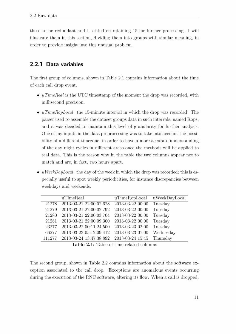
The first group of columns, shown in Table 2.1 contains information about the timeof each call drop event.

• uTimeReal is the UTC timestamp of the moment the drop was recorded, withmillisecond precision.

• uTimeRopLocal: the 15-minute interval in which the drop was recorded. Theparser used to assemble the dataset groups data in such intervals, named Rops,and it was decided to maintain this level of granularity for further analysis.One of my inputs in the data preprocessing was to take into account the possi-bility of a different timezone, in order to have a more accurate understandingof the day-night cycles in different areas once the methods will be applied toreal data. This is the reason why in the table the two columns appear not tomatch and are, in fact, two hours apart.

• uWeekDayLocal: the day of the week in which the drop was recorded; this is es-pecially useful to spot weekly periodicities, for instance discrepancies betweenweekdays and weekends.

uTimeReal uTimeRopLocal uWeekDayLocal21278 2013-03-21 22:00:02.628 2013-03-22 00:00 Tuesday21279 2013-03-21 22:00:02.792 2013-03-22 00:00 Tuesday21280 2013-03-21 22:00:03.704 2013-03-22 00:00 Tuesday21281 2013-03-21 22:00:09.300 2013-03-22 00:00 Tuesday23277 2013-03-22 00:11:24.500 2013-03-23 02:00 Tuesday66277 2013-03-23 05:12:09.412 2013-03-23 07:00 Wednesday111277 2013-03-24 13:47:38.892 2013-03-24 15:45 Thursday

Table 2.1: Table of time-related columns

The second group, shown in Table 2.2 contains information about the software ex-ception associated to the call drop. Exceptions are anomalous events occurringduring the execution of the RNC software, altering its flow. When a call is dropped,

11

Chapter 2 Data

an exception is raised in the RNC, and the type of exception gives valuable infor-mation on its cause.

• uEC is the software exception code that was reported in relation to the calldrop; it has a 1:1 correspondency with an explanatory string, which was re-moved due to redundancy. Each code corresponds to a different failure, rangingfrom expiration of timers to reception of error signals from various parts ofthe system. Over fifty unique codes are present in the dataset.

• uEcGroup is a grouping of the above codes that puts related exceptions to-gether into 15 categories; I requested this to be included so that collectiveincreases could be detected, on the hypothesis that related exceptions mighthave related causes.

uEC uEcGroup21278 43 INTERNAL_REJECT_AND_FAILURE_SIGNALS21279 42 INTERNAL_TIMER_EXPIRY21280 53 INTERNAL_TIMER_EXPIRY21281 43 INTERNAL_REJECT_AND_FAILURE_SIGNALS23277 27 EXTERNAL_REJECT_AND_FAILURE_SIGNALS_(RRC)66277 43 INTERNAL_REJECT_AND_FAILURE_SIGNALS111277 46 INTERNAL_TIMER_EXPIRY

Table 2.2: Table of software-related columns

The third group, shown in Table 2.3 contains information related to the geographicalarea in which the user device was located. In addition to the cell, higher levelgroupings were included to spot geographical patterns that might go unnoticed bylooking at a variable that is naturally very sparse (Over 800 different cell identifiersappear in the data).

• uCellId is the identifier of the cell the device was connected to. Cells areassociated with a stationary antenna, but there is no univocal correspondenceto location: a device is usually within range of multiple cells and the systemattempts to balance the load between them. Moreover, the serviced areacan expand or contract in size to balance the load (a process known as cellbreathing).

• kIubLinkName is an identifier for a higher level grouping, corresponding to theinterface between radio base stations and the RNC. One potential problem is

12

2.2 Raw data

that the mapping between cell and IubLink is not guaranteed to be fixed.Roughly 150 unique values appear in the dataset.

• kRncGroup is a yet higher level grouping; this is generally associated withIubLink and Cell, but this mapping too can potentially be redefined.

uCellId kIubLinkName kRncGroup21278 97 67 921279 171 32 2221280 677 16 1521281 513 107 1023277 77 135 2666277 531 33 20111277 829 79 9Table 2.3: Table of location-related columns

The fourth group contains information related to the type of connection that wasunexpectedly terminated.

• uUehConnType is a string indicating what type of connection was ongoing; theidentifier summarizes whether it was speech, data or mixed connection and thespeed of the data transfer.

• uUehTargetConn is a string indicating what connection was being switchedto: the system allows for connection types to be changed and it is common fordrops to happen in this phase.

• uUehConnTypeTransition is the concatenation of the two above strings; it isknown from expert knowledge that the aggregation can be more informativethan the two parts.

The fifth group contains information about the state of the connection that wasinterrupted. The process of setting up and maintaining a connection is very complexand the states represent various phases, most of them related to waiting for a specificsignal. A different thesis work carried out at the same time as this one was aimedat modelling these state transitions, following connections from start to end.

• uCurrentState is the state in which the connection was at the moment of thedrop. Over 100 distinct values are present in the data.

• uPreviousState is the state from which the connection reached the current one.Over 100 distinct values are present in the data.

13

Chapter 2 Data

The sixth group, shown in Table 2.4, contains information about the service thatwas interrupted by the drop.

• iuSysRabRel is a string reporting exactly which services were being offeredduring the connection (speech and/or packet data, at which speeds). Roughly50 unique levels are present.

• iuSysRabRelGroup is a grouping of the above, synthesizing the type of service:speech call alone, standard packet data alone, simultaneous speech and stan-dard data, high speed data, speech and high speed data, then legacy services(e.g. video calls sent as speech calls), for a total of 7 possible values.

iuSysRabRel iuSysRabRelGroup21278 18 PS_R9921279 32 PS_HSUPA21280 32 PS_HSUPA21281 32 PS_HSUPA23277 18 PS_R9966277 32 PS_HSUPA111277 32 PS_HSUPATable 2.4: Table of Service-related columns

2.3 Secondary data

One important part of information that is missing in the main dataset is the amountof connections that terminated without any problems: that is, how much normaltraffic was going on while the errors happened. This information is stored in adifferent source and it is therefore complicated to obtain it and synchronize it withthe errors dataset. Exploratory data analysis (see sec. 4.1.2) was carried out to judgewhether it was reasonable to include this data in the analysis.

14

3 Methods

As previously mentioned, this thesis work can be conceptually divided into two parts:the first, which I’ll refer to as detection, is concerned with finding time periods withanomalously high numbers of dropped call events and works with time series data;the second, which I’ll refer to as description, is concerned with characterizing eachanomalous period, comparing it with other periods that the detection has markedas normal and finding patterns that can be linked to specific failures.

3.1 Anomaly Detection

Detection is handled by analyzing the time series of dropped call counts, employinga model that can learn the usual amount of dropped calls and identify points inthe time series that deviate from learned behavior. An important consideration isthat the normal behavior of errors is closely related to the normal behavior of userson the network: there is a positive correlation between the amount of connectionsestablished and the amount of connections terminated unexpectedly. Since the ac-tivity of users of the network is expected to mirror daily routines and weekly cycles,any model applicable to this data has to have time as an input and account forperiodicity: what is normal during daytime might be extremely anomalous duringnighttime.

Works such as Weinberg et al. (2007) and Aktekin (2014) analyze similar data (call-center workload), however their focus is on studying normal behavior rather thanon considering anomalies. As we are working in an unsupervised context, whereunusual events are not labeled, learning a model of normal behavior is not straight-forward. Ideally we would like to remove abnormal events from the data beforetraining a model, but the meaning of abnormal itself depends on having a reliableidea of the baseline of normal behavior. This constitutes a circular problem thatwas likened to the ancient “chicken-and-egg” dilemma in the research paper that

15

Chapter 3 Methods

provided inspiration for this work. The chosen model deals with this problem bynot requiring the training set to be free of anomalies, building instead a concept ofanomaly in relation to other parts of the same time series. The technique, presentedin Ihler et al. (2007), utilises Poisson processes with variable mean to model countswhile accounting for periodicity, integrating a Markov state that represents whetheror not each time point is considered anomalous or normal. A posterior probabilityestimation of each time point being anomalous can be obtained by averaging theMarkov states over numerous iterations. Thanks to the Bayesian inference frame-work employed, this model can also answer additional questions about the data,for instance indicating whether or not all days of the week share the same normalbehavior.

Due to the completely categorical nature of the dataset and the practical obstaclesassociated with integrating potentially useful covariates (for instance the conditionsof the network, the signal strength or other sorts of continuous measurements relatedto connections), in this work detection operates on the time series alone.

3.1.1 Markov-Modulated Poisson Process (MMPP)

3.1.1.1 Basic Concepts

This technique models time-series data where time is discrete and the value N(t)represents the number of noteworthy events occurred in the time interval [t− 1, t];it was developed having in mind counts of people entering buildings and vehiclesentering a freeway and is therefore suitable for phenomena exhibiting the naturalrhythms of human activity. The model assumes that the observed counts N(t) aregiven by the sum of a count generated by normal behavior, N0(t), and another gen-erated by anomalous events, NE(t), as seen in 3.1. These two variables are assumedto be independent and modeled in separate ways, as described in the following twoparagraphs.

N(t) = N0(t) +NE(t) (3.1)

Periodic Counts Model (N0) The regular counts N0(t) are assumed to followa nonhomogeneous Poisson distribution, the most common probabilistic model for

16

3.1 Anomaly Detection

count data. The probability mass function (the density’s equivalent for discreterandom variables) in the standard case is

P (N0;λ) = eλλN0

N0! N0 = 0, 1, . . . , (3.2)

with λ being the average number of events in a time interval (rate), which is also thevariance. In the nonhomogeneous case, the constant λ is replaced by a function oftime, λ(t); more specifically in this case the function is periodic. The reasonablenessof the Poisson assumption must be tested on the data; in the nonhomogeneous case,this means testing separately each rate and the portion of the dataset associatedwith it (preferably after filtering out outliers). A common problem with Poissonmodels is that of overdispersion, when the sample variance is significantly higherthan the sample mean; the authors of Ihler et al. (2007) provide a qualitative way oftesting for this and state that this assumption does not need to be strictly enforcedfor the model’s purpose of event detection.

In order to model periodic patterns, λ(t) is decomposed multiplicatively as

λ(t) = λ0δd(t)ηd(t),h(t) (3.3)

with d(t) indicating the day of the week and h(t) the part of the day in which t

falls. λ0 is the average rate, δj is the relative day effect for day j (for instance,Mondays could have higher rates than Saturdays) and ηj,i is the relative effect fortime period i if day equals j. The constraints ∑7

j=1 δj = 7 and ∑Di=1 ηj,i = D (with

D being the number of subdivisions of a day) are imposed to make the parametersmore easily interpretable. Suitable conjugate prior distributions are chosen, specifi-cally λ0 ∼ Γ(λ; aL; bL) (a Gamma distribution), 1

7 [δ1, . . . , δ7] ∼ Dir(αd1, . . . , αd7) and1D

[ηj,1, . . . , ηj,D] ∼ Dir(αh1 , . . . , αh7) (two Dirichlet distributions).

Aperiodic, Event-Related Counts Model (NE) As seen in Equation 3.1 anoma-lous measurements are seen to be due to a second process, present only for a smallpart of the total time, which adds itself to the normal behavior. In order to indicatethe presence of an event, a binary process z(t), with Markov probability distribu-tion, is used. The process is the state of a Markov chain with transition probability

matrix Mz = z00 z01

z10 z11

, with each row having a Dirichlet conjugate prior; z = 0

17

Chapter 3 Methods

indicates no event and z = 1 indicates that an event is ongoing. z01 is therefore theprobability of an event occurring during normal behavior and z10 is the probability ofan ongoing event to terminate; the usual constraints on Markov transition matricesapply, therefore z00 = 1− z01 (probability of staying in a state of normal behavior)and z11 = 1−z10 (probability of an ongoing event to continue). The count producedby anomalous events can be modelled itself as Poisson with rate γ(t), written asNE(t) ∼ z(t) · P (N ; γ(t)) using the above definition of z(t). The rate γ(t) is drawnitself from a Gamma distribution with parameters aEand bE; this parameter canhowever be integrated over, yielding NE(t) ∼ NegativeBinomial(N ; aE, bE

(1+bE)).

The inclusion of a Markov chain, with its concept of state, allows the model toaccount for different types of anomalies; in addition to single counts that decisivelydeviate from the norm, the memory given by the state makes it possible to detectgroup anomalies, i.e. several values in a row that might not signify anything whentaken individually but could, as a whole, be indicative of an event.

3.1.1.2 Fitting the Model and Detecting Events

Assuming to know how N(t) is decomposed into [N0(t), NE(t), z(t)], it is easy todraw samples a posteriori of the parameters [λ0; δ; η;Mz]; this allows to obtain pos-terior distributions for them by inference using Markov chain Monte Carlo meth-ods. The algorithm alternates between drawing samples of the hidden data variables[N0(t), NE(t), z(t)] given the parameters and samples of the parameters [λ0; δ; η;Mz]given the hidden variables. Each iteration has O(T ) complexity, where T is thelength of the time series. As is customary with MCMC methods, initial iterationsare used for burn-in, while subsequent ones are retained in the results.

Sampling of the hidden variables proceeds in the following way: given λ(t) andMz asample of z(t) is drawn using the forward-backward algorithm (Baum et al., 1970).Then, given this hidden state, N0(t) is set as equal to the data value N(t) whenz(t) = 0 and drawn from a distribution proportional to

∑i

P (N(t)− i;λ(t))NBin(i; aE, bE

1 + bE) (3.4)

when z(t) = 1 (notice how this is weighed by the probability that the count N(t)− icame from the supposed Poisson distribution). This makes the model resistant to

18

3.1 Anomaly Detection

incorporating the anomalous events into its model of normal behavior: rather thansimply averaging over all the training data (obviously accounting for periodicities),which might lead to skewed normal counts if a massive event was registered, themodel adjusts downwards the contribution of counts that are deemed to be unusuallybig.

In case of missing data, N0(t) is drawn from the appropriate Poisson and NE(t) isdrawn independently. By writing out the complete data likelihood, it is possible toderive the distributions from which to draw the parameters given the data; becauseof the choice of conjugate prior distributions, the posteriors have the same formwith updated parameters obtained from the data; the detailed description appearson Ihler et al. (2007).

The presence or absence of events is coded in the model by the binary processz(t), thus the posterior probability p(z(t) = 1|{N(t)}) is used as an indicator ofwhen events occurred. This is obtained by averaging all samples of z(t) given by theMCMC iterations. A threshold Θ is then set to classify a time period t as anomalousif z(t) > Θ.

The prior parameters with the most influence over the performance of the modelare claimed by the authors to be the transition parameters of z(t), which regulatehow much the event process is allowed to compensate for high variance in the dataand thus possibly overfit; adjusting them obviously also affects the sensitivity andtherefore the number of events detected.

3.1.1.3 Testing differences between days

The model allows for each day to have its separate time profile, but that impliesa high number of degrees of freedom and as a consequence a high requirement onthe amount of data needed for training; however, it is possible to force some or allthe days to share their δ and ηi values: a separate profile can be learned for eachday of the week, two profiles can be learned for weekends and weekdays, or a singleprofile can be fit to all days. If the days that are grouped have similar behavior, thisleads to an easier to train, more robust model. It is possible to test whether the fullmodel or any constrained model is a better fit for the data by computing marginallikelihoods (likelihood of the data under the model, integrating out the parametervalues) as shown in 3.5. This is a particularly desirable characteristic of the model,as traffic data can exhibit different patterns depending on the geographical area

19

Chapter 3 Methods

from where the data is sourced and it is important to choose the best parametersdepending on the individual dataset.

p(N |constraintk) =�p(N |λ0, δ, η)∂λ0∂δ∂η (3.5)

This integral can be computed using the samples from the MCMC iterations; com-paring the likelihoods obtained under different constraints, both on δ and on η, itis possible to judge how much freedom to allow the model to have. Since the ex-pression contains the uncertainty over the parameters, there is no need to penalizeexplicitly a higher number of parameters.

3.2 Anomaly Description

Description deals with the actual multivariate categorical data; various techniquesare employed to correlate increases in the time series to changes in the underlyingdataset. Two main approaches are adopted, one extracting details about individualanomalies and another extracting common features among anomalies.

The first approach operates directly on the data; it uses the output of the timeseries detection to label specific time periods as anomalous and examines changesin the distribution of each categorical variable. Data from each anomalous period iscompared to data from related periods (previous and past days at the same hours)that are deemed to be normal, highlighting the specific attribute values showing asignificant increase; then techniques for anomalous pattern detection in categoricaldatasets, inspired by Das et al. (2008), are applied to test for correlations andinteractions between variables and select the patterns to output as a description ofthe anomaly.

The second approach, undertaken on the basis of the results of the previous anal-ysis, consists in selecting a subset of interesting variables and transforming thecorresponding data into a multivariate time series, with the aim of applying di-mensionality reduction techniques like PCA to gain a picture of the main trends.A simple anomaly detector, based solely on PCA, is then compared to the originalmodel in order to judge which methods would be suitable for integration in real-timemonitoring of the network.

20

3.2 Anomaly Description

3.2.1 Exploration of individual anomalies

Most of the anomaly detection literature concerning itself with multivariate data(for reference, see the review paper Chandola et al. (2009)) defines anomalies assingle points that are outliers in respect to the rest of the data, while collective,or group anomalies, are addressed much more rarely. Some of the techniques usedhere were presented in works aimed at detecting anomalous patterns; however, itwas decided to approach the detection otherwise because of the clear time-relatedpatterns present in the data and the domain-specific definition of anomaly as aperiod with higher counts regardless of the composition.

The exploration is carried out in two complementary steps: first, each categoricalvariable is examined separately, comparing the distribution in the anomaly withthat of the reference period; second, frequent pattern mining is used to identifyassociations between specific categorical values across different variables (sets ofvalues appearing together), as in Brauckhoff et al. (2012).

For each anomalous period (a continuous stretch of 15-minute intervals flagged asanomalous) the corresponding portion of the call drop dataset is extracted; in orderto provide a reference dataset to compare against, each of these portions is associatedto a reference dataset, made up of data from the same time period in different days.For instance, if an anomaly is detected on Day 10 between 15:00 and 16:00, thereference will be built with the same hour between 15:00 and 16:00 from Day 9, 8, 7and so on, skipping days that contain anomalies themselves. The number of referencedays affects the data size of the reference period and therefore the time needed forcomputations; a balance needs to be struck between having an accurate picture ofthe normal activity and getting results quickly. A maximum amount of referencedays is set depending on the amount of data available and on assumptions about itshomogeneity (if the dataset is small or there is concern that normal patterns mightbe changing, a lower amount is preferable).

3.2.1.1 Comparing distributions

The basic idea, borrowed from Kind et al. (2009), involves selecting a few variables(each representative of one of the groups outlined in sec. 2.2.1) and representing thedistribution of drop events by constructing a histogram for each of them, using thepossible attribute values as bins; then histograms from anomalous periods (showing

21

Chapter 3 Methods

the count of records having the respective value in the period) are compared tohistograms from the reference data (showing the average number of appearances ofthe same attribute in the reference periods). Probabilistic measures of differencebetween distributions, such as the Kullback-Leibler divergence found in Brauckhoffet al. (2012), were discarded because they emphasize relative, rather than abso-lute, differences, and are not defined when the support of the two distributions isnot overlapping (in cases where some attributes only appear during the anomalousperiod, they are assigned probability 0 in the normal data: this yields an infinitedivergence regardless of the number of occurrences, which is undesirable).

The comparison is based on a simpler measure, the Manhattan distance. Repre-senting a portion of the original dataset labeled as anomalous with p, rows of theoriginal dataset as rj and choosing a categorical variable a, having n possible valuesα1, α2, . . . , αn,

x = (x1, x2, . . . , xn) is the histogram for p, with xi = #(rj ⊂ p : aj = αi).

Similarly, a histogram y can be defined for the same variable in the reference data.Representing the m chunks of data taken for reference as qk (k ∈ [1,m]), we canwrite

y = (y1, y2, . . . , yn), with yi = 1m

∑mk=1 #(rj ⊂ qk : aj = αi)

A second vector s = (s1, s2, . . . , sn) is then computed for the reference period, withsi the standard deviation on each of the averages yi across the m subsets.

Then di = |xi − yi| is the contribution from attribute i to the Manhattan distancebetween the two histograms d = ∑n

i=1 |xi − yi| and ti = di

siis a score of how unusual

the deviation is. Attribute values whose absolute and relative deviation scores diand si are higher than specified thresholds are reported (thresholds for si can bedetermined with the same criteria as a statistical test, while thresholds for di dependon the level of detail desired by the user).

Variables with special treatment A particular treatment was reserved to thevariables corresponding to the geographical location of the records. The interest-ing aspect is to determine whether or not the problems are confined to a specificsubdivision of the network: if the problem is happening at the center of the net-work, many areas will see increases which are not ultimately interesting. Thereforeit is sensible to introduce a measure of the concentration of the distribution across

22

3.2 Anomaly Description

these variables: the kurtosis, computed on x as µ4x

σ4x− 3, was chosen empirically as it

correlated well with expert judgment.

3.2.1.2 Frequent pattern mining and co-occurrences

The previous step returns a list of abnormal attribute values for each individualvariable, but the transformation of the data in histograms hides the underlyingstructure of each row. The most suitable techniques to uncover subsets of nominalvalues appearing frequently together in the same row belong to the family of asso-ciation rules/frequent patterns mining, originally defined in Agrawal et al. (1993).Specifically, the example of Brauckhoff et al. (2012)was followed, using the Apriorialgorithm to obtain maximally frequent itemsets (that is, itemsets whose supersetsare not frequent); the amount of patterns output can further be reduced by onlyincluding those that contain values selected as anomalous in the previous step.

Seen that many frequent patterns are not specific to the anomalous period but alsoappear in the reference data, another filtering step of this output may be useful: asseen in Das et al. (2008), the support of each candidate pattern is computed also inthe reference dataset, obtaining a 2x2 contingency table. Then, Fisher’s exact test(Fisher, 1922) is applied to this table, to judge if the pattern is significantly morecommon in the anomalous data and therefore characterizes it.

In order to compute the support of the patterns in the reference data, where theymay not be frequent, the standard algorithms were unsuitable; the cited work em-ploys a dedicated, optimised data structure for computing contingency tables. Giventhe manageable data size, it was decided to adopt a simpler approach, described inHolsheimer et al. (1995), better suited to quick coding in the R environment. Thedata is transformed from the usual row-based format, where the value of each vari-able in the row is shown, to the dual representation of TID-lists: TID stands fortransaction identifier and each TID corresponds to a row. Each possible attributevalue is assigned a list of the rows it appears into; in order to obtain the rowsin which a group of attributes appear together, it is sufficient to perform the setintersection of the respective TID lists, and simple counting yields the support.

Given the nature of the data, the amount of frequent patterns returned as outputgrows rapidly as more variables are added, therefore a small number of main columnswas chosen for this step; another requirement was to then be able to inspect theassociation of the main variables with others that were otherwise disregarded. This

23

Chapter 3 Methods

was implemented similarly to frequent pattern mining, taking as input the specificsets of values to examine and using TID lists to explore their co-occurrences. Inaddition to the aforementioned statistical testing on the support, a measure of theconfidence of each co-occurrence was computed: with A being the value of the mainvariable and B that of the other, conf = Support(A ⇒ B)/Support(A), in otherwords how many of the records containing A also contain B (in association rulemining, the support of a rule is the number of records in the dataset that containthe rule). This will be useful for instance to determine if any single user is causinga significant proportion of the dropped calls in a geographical area, as this mayindicate that the problem lies in the user device rather than in the network.

3.2.2 Dimensionality reduction and extraction of main patterns

The above techniques extract automatically interesting details about anomaloustime periods, which are potentially useful for in-depth analysis of root causes andongoing problems for the network or for subsequent correlation with other datasources in the network; however, it is also desirable to obtain quick, summary infor-mation of the main features of anomalous data. Dimensionality reduction techniquesoften prove very useful in unsupervised problems of this kind; however the most com-mon ones, such as Principal Component Analysis, are not applicable to categoricaldatasets such as this one. In order to overcome this constraint, it was necessary totransform the data, in the process losing information about the structure of individ-ual rows. Each categorical column was transformed into a set of indicator variables,one for each possible value, and the indicators were summed for every 15-minuteperiod, obtaining a multivariate time series: structure is lost as it is infeasible toadd terms for all the possible combinations of attributes appearing in the same row.Regression techniques having the total count for each period as output would bemeaningless, as the response is simply given by adding all the counts for one vari-able; on the other hand, correlation analysis and PCA can show which attributes,both within the same variable and across different variables, grow together. Someprincipal components can then be associated to the normal behavior, while oth-ers encode spikes, local increases and other deviations; the attractiveness of PCAlies in the fact that it is possible to interpret the loadings in order to understandwhich variables influence each principal component score, and correlated variablescontribute to the same component. Thus, a big component score corresponds to an

24

3.3 Technical aspects

extreme value of its contributing variables and it is possible to label anomalies inthe total count according to the principal components that have high values.

In order to make PCA loadings easier to interpret, it is possible to apply the vari-max rotation (Kaiser, 1958), a transformation that, while maintaining orthogonality,yields loadings with very high or very low coefficients, associating most variables toa single loading. This trades some precision in the representation for higher inter-pretability of the scores, with the latter being more desirable in this specific usecase.

It is important to note, however, that the PCA approach does not retain the timecomponent of the data: the time series is seen simply as a multidimensional dataset,with no importance given to the order of the rows, thus limiting the ability torecognize abnormal behavior that is only anomalous in relation to the time duringwhich it happens.

3.3 Technical aspects

This thesis work has been carried out using the R programming language and soft-ware environment; Unix command line utilities were employed for data cleaning,pre-processing and subsetting in order to keep the data to a manageable size - theoriginal, raw comma-separated values file weighing 2 GB. For the MMPP algorithm,I rewrote into R the MATLAB code released by the authors of Ihler et al. (2007),testing its results on the enclosed example datasets. The ggplot2 plotting library wasused for graphics, employing a “color-blind-friendly” palette, and frequent patternmining relied on the apriori R package.

25

4 Results

4.1 Exploratory analysis

4.1.1 Main data

As previously mentioned, the standard way to study this data in the time domain isto look at the count of drops in every 15 minute period; this was maintained throughmost of the analysis. The time series is shown in Figure 4.1. The daily periodicity isimmediately noticeable in Figure 4.2, with lower counts in the early hours of the dayand peaks in the evenings; several spikes of various magnitudes are present, with aconcentration during a week on either side of the fifth Sunday, during which everyday presents an abnormal peak as compared to the rest of the time series. Figure 4.3shows in higher detail a week-long portion of the data; each of the first four dayspresent spikes in which the drop count reaches up to 5 times the usual values. Thepeaks appear at irregular times, even during the nighttime. Other, much smallerspikes can be seen in other days, while the overall pattern appears quite regular,with small differences between the overall shapes of days.

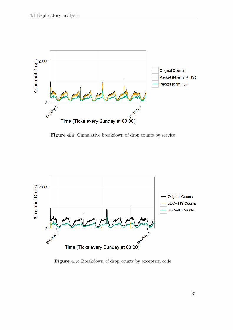
One important consideration to make is that the categorical data can be seen ascompositional data: by transforming each categorical variable into a set of indicatorvariables, one for each possible value, and compressing the information into countsevery 15 minutes, we will obtain a time series of counts, with the constraint thatthe total count shown in Figure 4.1 is always equal to the sum of the counts ofthe indicators for any one of the variables. This is shown in Figure 4.4, using theservice group variable, showing how most of the dropped traffic is either normal orhigh-speed packet data (mobile internet).

By breaking down the total count into its parts, however, an increase in the total timeseries will correspond to increases in some categories for every variable; discerningwhich variables actually contain valuable information about the nature of the event

27

Chapter 4 Results

Figure 4.1: Time series of dropped call counts every 15 minutes.

that caused the increase would be desirable but is not always possible, even fordomain experts.

Figure 4.5 shows how similar spikes can have very different underlying data; picturedin green are the counts of drops reporting one of the most common exception codes,40, while in yellow is a rare code, 119. The spike on the fifth day corresponds toa raise in frequency of exception 40, while spikes on the seventh and first days areassociated to a burst of the rarer 119 exception; yet another spike, on the third day,does not correspond to any of the two. This is a good example of a variable that givesvaluable information: looking at service types the spikes are indistinguishable, whilethe exception code graph shows that two of them are associated with an uncommonlyhigh number of occurrences of a specific exception. It would then be interesting tofind out if these exceptions happen only with a specific type of connection or in aspecific part of the network; this has been one of the focal points of this work.

28

4.1 Exploratory analysis

Figure 4.2: Detail of a regular day, showing the daily pattern

4.1.2 Secondary data

Another goal of the exploratory analysis was to understand whether or not it wasnecessary to include information about the amount of normal connections for everygiven time period, which is stored in a different data source, in order to understandthe normal behavior and judge how necessary the integration of this source is. FromFigure 4.6 it can be seen how the normal connection counts, in blue (rescaled in orderto have the same magnitude as the abnormal ones) appear much more regular thanabnormal drops counts, with only a few spikes of much smaller relative magnitude.Also, it can be seen how the amplitude of the oscillations is different, suggesting thatthere is a dependency between normal connections and abnormal drops: in otherwords, the ratio of connections that drop is not normally constant but dependson the amount of traffic on the network. This was tested with a simple linearregression, having the number of normal connections as dependent variable andnumber of abnormal drops as response variable, yielding a significant slope (theresulting plot appears in Figure 4.7). The presence of many outliers means that thestandard assumptions for linear regression are violated, but this analysis is enough

29

Chapter 4 Results

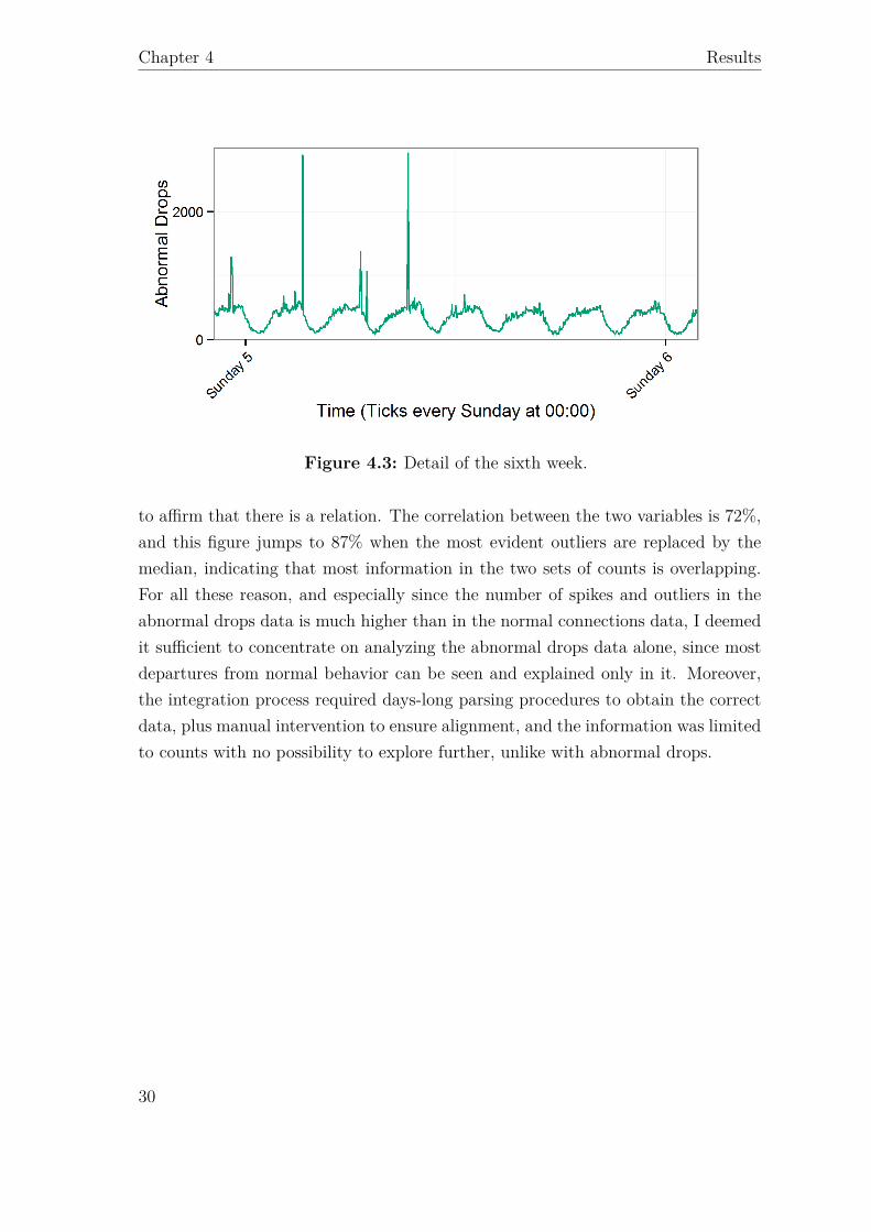
Figure 4.3: Detail of the sixth week.

to affirm that there is a relation. The correlation between the two variables is 72%,and this figure jumps to 87% when the most evident outliers are replaced by themedian, indicating that most information in the two sets of counts is overlapping.For all these reason, and especially since the number of spikes and outliers in theabnormal drops data is much higher than in the normal connections data, I deemedit sufficient to concentrate on analyzing the abnormal drops data alone, since mostdepartures from normal behavior can be seen and explained only in it. Moreover,the integration process required days-long parsing procedures to obtain the correctdata, plus manual intervention to ensure alignment, and the information was limitedto counts with no possibility to explore further, unlike with abnormal drops.

30

4.1 Exploratory analysis

Figure 4.4: Cumulative breakdown of drop counts by service

Figure 4.5: Breakdown of drop counts by exception code

31

Chapter 4 Results

Figure 4.6: Overlapping abnormal drops and normal connections

Figure 4.7: Scatterplot of abnormal drops versus normal connections, with linearregression line

32

4.2 Detection of anomalous periods using the MMPP model

4.2 Detection of anomalous periods using the MMPPmodel

4.2.1 Preprocessing

Fitting the MMPP model on data in the original scale presented problems with theconvergence of the algorithm: due to the equivalence between mean and variance,the distribution becomes more and more flat as the mean increases. This meansthat the likelihood obtained with the “correct” mean that the algorithm estimatesis similar to those obtained with slightly different mean values, causing the algorithmnot to converge stably on its λ values and therefore impacting all other inference.Adjusting prior parameters did not relieve this problem, but a simple rescaling of thedata eliminated the problem: all counts were divided by a constant K and roundedto the nearest integer, and model fitting was performed on the resulting time series.Eventually K = 10 was chosen as it is intuitive to grasp the original scale withpowers of 10, the detection results were satisfying and a rounding of this magnitudedid not lose any interesting details, as noisy variations in the data are themselvesbigger. Figure 4.8 shows detection results on the original time series, with immediateevidence of non-convergence. An added benefit of rescaling is that it lowers themean-to-variance ratio, which reduces problems related to overdispersion of the data(a common problem with Poisson models as they do not allow to specify mean andvariance separately); once anomalous points are removed, the mean/variance ratioswere computed separately or each of the 96 15 minute periods in a day, which areassumed come from the same distribution, yielding values between 1.2 and 3.8, rulingout overdispersion.

4.2.2 Choice of parameters

Once transformed the data to a suitable scale, the first step of fitting the MMPPmodel involved choosing how many degrees of freedom to allow for the normalbehavior: the assumption from the data providers was that weekends would besignificantly different from workdays, while the above plots only seem to suggestdaily, rather than weekly patterns. The MMPP model was therefore fit to thedataset with various constraints on the day and time of day effects: each day withthe same profile, different profiles for weekends and weekdays and different profiles

33

Chapter 4 Results

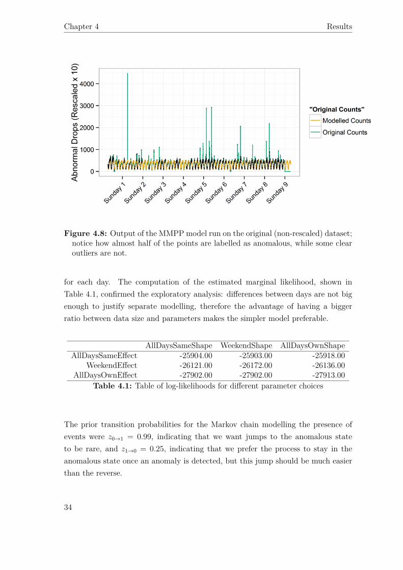
Figure 4.8: Output of the MMPP model run on the original (non-rescaled) dataset;notice how almost half of the points are labelled as anomalous, while some clearoutliers are not.

for each day. The computation of the estimated marginal likelihood, shown inTable 4.1, confirmed the exploratory analysis: differences between days are not bigenough to justify separate modelling, therefore the advantage of having a biggerratio between data size and parameters makes the simpler model preferable.

AllDaysSameShape WeekendShape AllDaysOwnShapeAllDaysSameEffect -25904.00 -25903.00 -25918.00

WeekendEffect -26121.00 -26172.00 -26136.00AllDaysOwnEffect -27902.00 -27902.00 -27913.00

Table 4.1: Table of log-likelihoods for different parameter choices

The prior transition probabilities for the Markov chain modelling the presence ofevents were z0→1 = 0.99, indicating that we want jumps to the anomalous stateto be rare, and z1→0 = 0.25, indicating that we prefer the process to stay in theanomalous state once an anomaly is detected, but this jump should be much easierthan the reverse.

34

4.2 Detection of anomalous periods using the MMPP model

4.2.3 Output

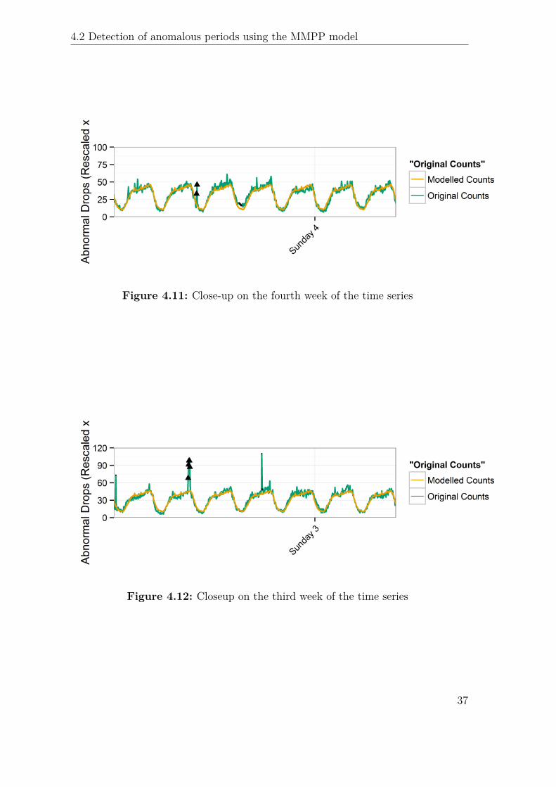
The estimated probability for each of the 5856 time points, obtained with 10 burn-initerations, 100 sampling iterations and considering all days to have the same pro-file, is shown in Figure 4.9. For subsequent analysis, it was necessary to translatethis probability in a binary decision rule; the choice was to consider points withP (anomaly) > 0.5 as anomalous. The 0.5 threshold was preferred to the moreconservative 0.95 as the latter would exclude some group anomalies that, due tothe stochastic nature of the method, were not detected reliably at every iteration.Figure 4.10, Figure 4.11 and are closeups on week-long sections of the data, demon-strating how both short-term, spike anomalies and smaller, continuous deviationsfrom the normal behavior are successfully detected. 289 of the 5856 data points arelabelled as anomalous, grouped in 37 sequences. 30 are less than two hour long (8or less points), 5 are between 2 and 5 hours and the remaining 2 are 13 and 19 hourslong.

Figure 4.9: Plot showing the estimated probability of anomaly for each time point

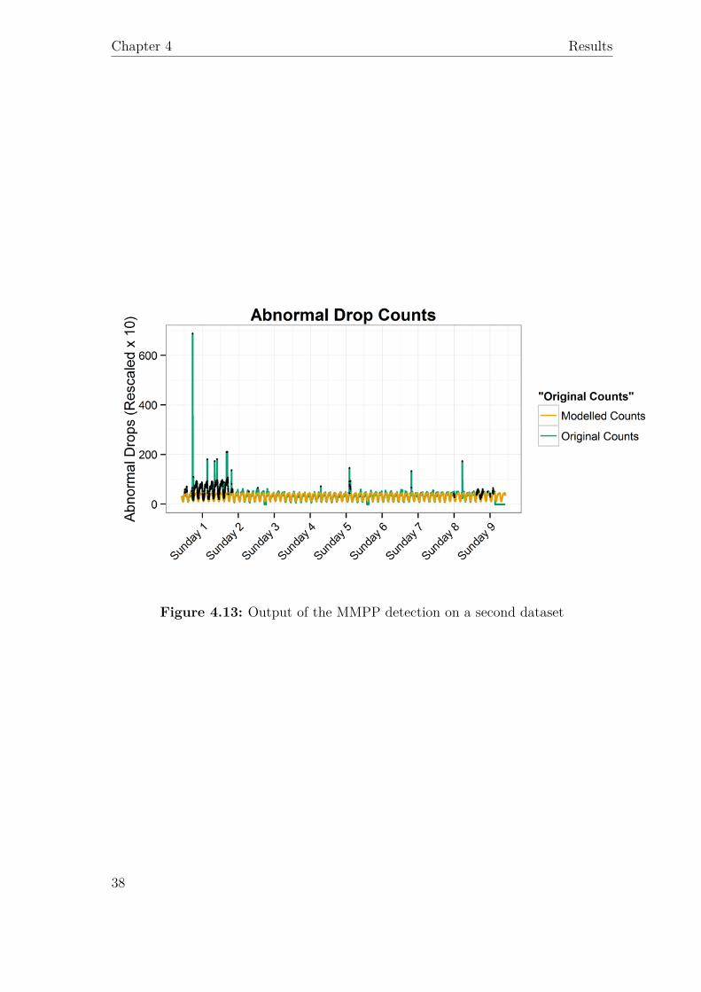
In addition to the main dataset, a time series extracted from another dataset wasalso available. The output is shown in Figure 4.13; this data had a different nature,with the first days exhibiting very different behavior with respect to the rest of the

35

Chapter 4 Results

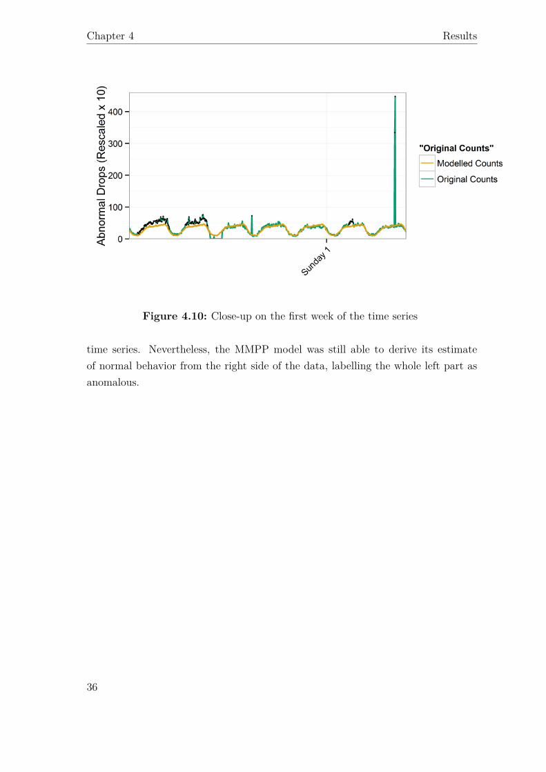
Figure 4.10: Close-up on the first week of the time series

time series. Nevertheless, the MMPP model was still able to derive its estimateof normal behavior from the right side of the data, labelling the whole left part asanomalous.

36

4.2 Detection of anomalous periods using the MMPP model

Figure 4.11: Close-up on the fourth week of the time series

Figure 4.12: Closeup on the third week of the time series

37

Chapter 4 Results

Figure 4.13: Output of the MMPP detection on a second dataset

38

4.3 Exploration of anomalous periods

4.3 Exploration of anomalous periods

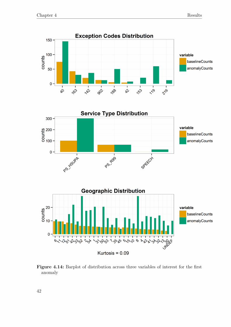
In the following section, output regarding two anomalous time periods is presented;the techniques used are intended to summarize information for an expert user, whocan then rule out or confirm own hypotheses about the cause of the problem. Onlya subset of the analysed variables (already a subset of the available ones) is pre-sented here. The first is the spike marked with triangles on the left-hand side inFigure 4.11, occurring during nighttime with a duration of less than 30 minutes (no-tably, the count wouldn’t have been considered anomalous if occurring during theevening), reported in Table 4.2. Three exceptions and one service type are reportedas meaningfully deviating, while nothing is reported about geographical distribu-tion, since the flat shape suggests a problem happening centrally in the networkcontroller. Barplots for the three variables are reported in Figure 4.14.

Frequent pattern mining, run on 4 variables with a 2.5% threshold on support, re-turned 98 patterns. Inspection of the output, which is not included for brevity,allows to see that code number 119, making up 15% of the total drops, is associatedwith high-speed data (PS_HSUPA) and speech calls (SPEECH), but not with stan-dard data (PS_R99); that specific exception code never appeared in the referencedata, therefore its expected frequency is 0 and all frequent patterns that include itare significant for the Fisher check on the ratio. As for code number 40, despitean increase in the overall number, the ratio in the anomalous period is 36% againstthe normal 44%, as the emergence of a large amount of records with different codesinflates the denominator; this means that most patterns involving code 40 do notpass the Fisher test. Without careful interpretation, this may give a distorted pic-ture of the situation, but the benefit is that the most interesting patterns, thosethat increased in frequency in line with the overall increase of dropped calls, arehighlighted. In this case, the only reported pattern involves a specific connectiontransition (C_TO_D), which can be singled out for further analysis as it appearsto be one of the symptoms of the event that has caused an increase in the amountof dropped calls. Looking at the confidence analysis, the confidence of encounteringC_TO_D given all the drops with exception 40 went from 20% to 40%, confirmingthat the increase was meaningful; this is given as an example of the possible relationsthat can be quickly checked by inspecting the description output. As will be dis-cussed in chapter 5, only integration with other datasets and contribution of expertknowledge can lead to a better automation of the interpretation of these results; it

39

Chapter 4 Results

appears clear, however, that this fault has its origin in the central system, showingerrors that are never seen during normal operation.

Variable Value Reference StDev Anomaly Score1 uEC 40 75.20 21.30 145.50 3.302 uEC 119 0.00 0.00 60.00 Inf3 uEC 188 5.20 2.30 50.50 19.807 iuSysRabRelGroup PS_HSUPA 101.60 25.60 301.50 7.80

Table 4.2: Table of deviating values for the first period

The second is the spike marked with triangles during the second day of Figure 4.12,occurring in the evening with a duration of 5 time points (between 60 and 75 min-utes); its summary is reported in Table 4.3. Here 2 exception codes and 2 servicetypes are reported, but the most interesting aspect is that a single grouping in thenetwork controller, corresponding to a few cells of the network, reported as manydrops as the rest of the network combined, and was the sole responsible of theanomaly: the total average number of drops went from 458 to 883 (a difference of425) while the specified geographic area went from 14 to 415 (a difference of 401,almost as big as the total increase). Barplots for the three selected variables areshown in Figure 4.15, the last being especially interesting as it demonstrates howconcentrated the anomaly was.

Frequent pattern mining, run with the same parameters, returned 80 patterns; pat-terns including the anomalous geographic area show how all main service typesare affected, as well as one exception code, 902, that is the third most frequentin that area and only the fifth overall. More interesting is the related analysis ofco-occurrences, which allows to see how the main geographic subdivision variable,kRncGroup, correlates with others in the same group. Two cells with consecutiveidentifiers, indicating close geographical proximity, are responsible for 95% of thedrops reported in the specific RncGroup: in a real setting this could indicate thata concentration of many people inside the coverage area of the antennas has led toan overload of the network, with a subsequent impact on its ability to retain phonecalls. In that case the blame for the decrease in performance could be attributed toexternal factors; if multiple such events were reported it would be advisable to in-vestigate the causes and possibly install more antennas in the area. However, therewere no other anomalies regarding those cells in the dataset.

40

4.3 Exploration of anomalous periods

Variable Value Reference StDev Anomaly Score1 uEC 40 223.10 13.20 492.20 20.402 uEC 163 81.80 9.70 137.80 5.803 kRncGroup 15 13.70 4.80 415.80 84.208 iuSysRabRelGroup PS_HSUPA 259.90 19.70 519.20 13.209 iuSysRabRelGroup PS_R99 178.10 11.10 337.80 14.30

Table 4.3: Table of deviating values for the second period

41

Chapter 4 Results

Figure 4.14: Barplot of distribution across three variables of interest for the firstanomaly

42

4.3 Exploration of anomalous periods

Figure 4.15: Barplot of distribution across three variables of interest for the secondanomaly

43

Chapter 4 Results

4.4 Analysis of main patterns common to anomalousperiods

The findings of the previous steps allowed to select some interesting variables, aswell as features obtained from others, that can summarize the main interestingpatterns of behavior in the data; these were transformed in a multivariate timeseries, as described in sec. 3.2.2. Exceptions and service types related to phone callswere retained, eliminating attributes appearing less than 50 times in the 2 millionrows; then two new variables were added: NoConnChng, the amount of drops notassociated with a transition between connection types, andMaxRncMod, the numberof drops in the busiest area at every time step. Plotting the correlation matrix ofthe resulting 39-dimensional dataset, with rows ordered by hierarchical clustering(a common visualization technique) confirms some previous intuition: the bulk ofexception codes (from 221 to 188) can be thought of as having similar origin, as theyshow quite big correlations between them. All the main, most frequent exceptions,which are found in all periods, belong to this group. Then in the bottom right cornerthere is a group of exception codes that are in many cases (including one of the twopresented in sec. 4.3) unique to anomalous periods, and characterize a subset of allanomalies. These show very strong correlation, indicating that they are likely torepresent the same underlying phenomenon, and are strongly associated with losingphone calls (these are prioritised during normal operation and it is intuitive thatthey are only dropped in large numbers when a severe problem happens). Othersmaller groups exist, for instance two codes that correlate with high activity in ageographical area and therefore may indicate congestion, and there are also a fewcodes that seem to be completely unrelated to others, for example because theyappear only once in a big spike (87).

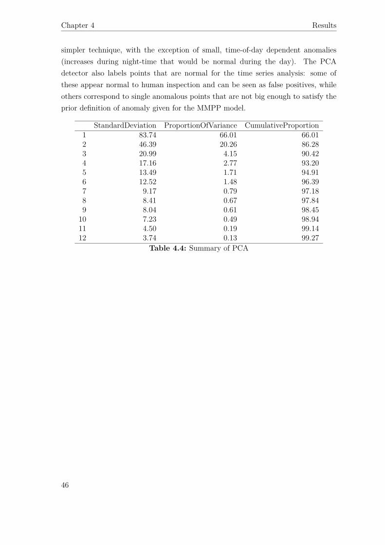
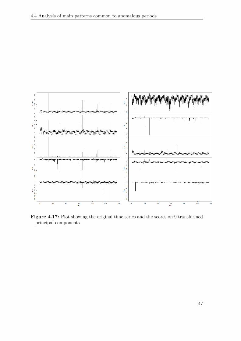
PCA can be expected to summarize the structure of the data; in order to retain in-formation on the size of the variables and prioritize more frequent attributes (whichhave higher counts) it was decided to run the algorithm on unscaled data using thecovariance matrix; this is legitimate as all variables have the same scale. Results ofthe PCA are shown in Table 4.4; as the proportion of variance explained decreasessubstantially around the 10th component, following components can be discardedwithout loss of interesting information. By inspecting the PCA scores, it is clearthat the first principal component accounts for the main daily pattern in the timeseries, while subsequent components capture deviations. Since the main focus of

44

4.4 Analysis of main patterns common to anomalous periods

Figure 4.16: Correlation matrix between time series of appearance counts of chosenattributes

the work is to obtain easily interpretable results, the scores obtained after applyingthe varimax rotation to the first 9 components are reported (see Figure 4.17); thefirst component corresponds to the most common exception, 40, while the secondcaptures 119, 153 and SPEECH drops, the most important members of the clusterin the correlation plot. The third component corresponds to the cluster of vari-ables related to congested cells; 4th, 5th and 7th capture other variables relatedto common exception codes, the 8th some interaction between common and burstyexceptions, while 6th and 9th correspond to rarer bursty exceptions (missing dataand exception code 87 respectively).

A simple anomaly detector is constructed using these 9 scores, by labeling a pointas anomalous for a component if its score is more than 3 standard deviations offthe mean (which is always zero); the results in Figure 4.18 show how most of theanomalies shown by the more complex time series model are also captured by this

45

Chapter 4 Results

simpler technique, with the exception of small, time-of-day dependent anomalies(increases during night-time that would be normal during the day). The PCAdetector also labels points that are normal for the time series analysis: some ofthese appear normal to human inspection and can be seen as false positives, whileothers correspond to single anomalous points that are not big enough to satisfy theprior definition of anomaly given for the MMPP model.

StandardDeviation ProportionOfVariance CumulativeProportion1 83.74 66.01 66.012 46.39 20.26 86.283 20.99 4.15 90.424 17.16 2.77 93.205 13.49 1.71 94.916 12.52 1.48 96.397 9.17 0.79 97.188 8.41 0.67 97.849 8.04 0.61 98.4510 7.23 0.49 98.9411 4.50 0.19 99.1412 3.74 0.13 99.27

Table 4.4: Summary of PCA

46

4.4 Analysis of main patterns common to anomalous periods

Figure 4.17: Plot showing the original time series and the scores on 9 transformedprincipal components

47

Chapter 4 Results

Figure 4.18: PCA anomaly detector (colored squares) compared to MMPP detec-tor (black dots)

48

5 Discussion

To our knowledge, this thesis work has been the first data mining approach toanomaly detection in the specific type of dataset considered; as such, it can be seenas a pilot test of suitable methods, rather than a thorough, definitive solution tothe problem. Prior to this, there was little systematic knowledge of what could beinteresting hypotheses to test or informative patterns to find; for this reason, it waspreferred to explore various techniques, some proving more effective than others,rather than develop extensively a single method. Another element that complicatedthe choice of the methods was the format of the dataset: having originally beendeveloped for inspection with spreadsheet software, this data is not readily com-parable to what is commonly analyzed in standard literature. Works on similardatasets exist and were used as inspiration, but differences were sufficiently big thatit was not possible to simply replicate their methodology.

A large amount of time was spent on understanding the data, determining whichtechniques showed the most promise and which features were worthy of being re-tained; goals constantly shifted every time the methods revealed more about thestructure of the dataset. For instance, a requirement that appeared to be very im-portant at the start was to be able to analyze many variables, which led to theinclusion of pattern mining and co-occurrences analysis as a big part of the work.

However, after examining the output it became clear that anomalies could be moreeasily characterised with simpler methods, while frequent patterns provide addi-tional information that is only useful when analyzing the details. These techniqueswere retained as a helpful analysis tool, to improve the way in-depth analysis isperformed by troubleshooters, but ultimately contribute a smaller part of the in-teresting results than originally expected. Histogram analysis itself was originallyconsidered as a tool to detect anomalies, before turning into one of the more easilyinterpretable exploratory techniques; using the Manhattan distance, despite it beinga relatively crude approach compared to a statistical divergence, made it possible to

49

Chapter 5 Discussion

focus on the single attribute values that define anomalies and are ultimately moreimportant to the end goal of the work.

Despite not being exhaustive or systematic, histogram analysis and pattern miningwere nevertheless very useful for understanding the dataset and selecting interest-ing features for further analysis. Among the 37 anomalous periods found in thedevelopment dataset, the analysis exposed many different patterns, from geographi-cally concentrated episodes to central failures. Even though various periods showedunique characteristics, common features to many anomalies were identified, in termsof exception codes present and areas affected.

Having mentioned exploratory techniques, it is time to comment on the other meth-ods employed in this work. Specifically, the MMPP method was able to give a solid,understandable foundation with which other, more empirical methods could be com-bined and compared; nevertheless, some considerations have to be made about itseffective applicability in automated analysis. One possible problem regards its suit-ability for continuous monitoring of the data: the algorithm in its current form doesnot work on-line, therefore it has to be retrained every time new data is added.Also, the concepts it is based on are quite sophisticated and a substantial amount ofdata is required for training; as the data was found to be quite regular, it might besensible to consider substituting the model with a simpler, threshold-based modelbuilt using the insight gained from MMPP. The resulting model would be less pow-erful or attractive from a purely statistical viewpoint, but it could prove faster andeasier to maintain. One indication of the aforementioned regularity of the data wasthe fact that the estimated λ computed by the MMPP model for each 15-minutepart of the day and the median of the corresponding population had a correlation of0.9992, proving both that the inference was working well and that a much simplertechnique would have given a good estimate of the expected normal frequency of calldrops. However, as new datasets are collected and tested, the need for flexibility ishighlighted: in many cases, significant differences between workdays and weekdayscan be observed, confirming the validity of choosing a more complex model such asMMPP.

Regarding the PCA techniques, they were the ones that showed the biggest poten-tial of solving with a single method the two problems of detecting anomalies andunderstanding them; unfortunately they were introduced late in the development ofthe work, as for a long time it appeared more important to retain the full structure

50

Discussion

of the data and operate on the categorical database itself, and therefore they couldnot be fully developed. More attention would have to be devoted to choosing theright parameters and settings, for instance whether or not to scale the data (scaleddata gave better prediction but complicated interpretation) and how to constructthe anomaly detector from the component scores. These decisions would requirea more thorough literature review, as well as extensive testing on more datasets;the recent emergence of datasets with more complex patterns of normal behavior,while strengthening the case for choosing the MMPP model, further complicatesthe adoption of the PCA approach as a possible single solution. Canonical Correla-tion Analysis was also briefly considered as an alternative to PCA, and ultimatelydiscarded due to longer processing times that made tuning parameters and assess-ing results infeasible during the late stage of development of this work; this mightrepresent an interesting future development.

As for implementation, which is ultimately an important practical concern, the per-formance achieved is undoubtedly satisfying: execution of the full stack of developedR scripts, on a single Intel Core i5-3427U 1.8 GHz CPU, takes less than 15 minuteson a dataset of about 2 million rows and 388 megabytes of compressed size. Thisallows for deployment of the methods in automated analysis without having to mi-grate the code to faster programming languages and indicates how the R coding inthis thesis has been efficient.

A final consideration to be made is that having separated anomaly detection fromsubsequent description makes it possible to use the database mining techniques forother, related tasks. For instance, it is often desirable in troubleshooting to comparetwo pre-defined periods of time, searching for the emergence of new patterns broughton by system changes or new user devices. Collection of data for this purpose is stillunderway, therefore this use case cannot be reported here, but the techniques havebeen developed to be readily adaptable.

51

6 Conclusions

With this work being, to our knowledge, the first step towards applying data miningto troubleshooting of dropped calls, it is important to focus the conclusion on thewider picture and the work ahead. Evaluating results on their own is complicated,mostly due to a lack of ground truths to be used for comparison - a situation commonto many unsupervised learning problems.

In this case, those ground truths could be found either by human evaluation of manysample datasets or by correlation with other data sources. The former is currently avery time-consuming operation, but this work can accelerate it by bringing interest-ing patterns to the attention of the domain expert. The latter is a very interestingand promising possibility for future development, moving towards a wider adoptionof data mining techniques in troubleshooting.

However, the associated challenges cannot be underestimated: in the context of acompany managing huge systems, obtaining and integrating data is very complex.This thesis has developed methods to extract interesting features from one datasource; once they have gained acceptance, it will be possible to set up joint monitor-ing of the same network with different tools and compare anomalies in dropped callswith changes in performance reporting. Another interesting development would beto follow the calls which we see are dropping from the beginning, as was done inZhou et al. (2013), to understand the phenomenon in a way that cannot be achievedwith this dataset alone.

To sum up, while the methodologies proposed are by no means exhaustive, thiswork has succeeded in leading to a better, more systematic understanding of theproperties of dropped calls data, paving the way for further analysis which will beable to benefit from integration with other datasets.

53

Bibliography

Agrawal, R., Imieliński, T., and Swami, A. (1993). Mining association rules betweensets of items in large databases. SIGMOD Rec., 22(2):207–216.

Aktekin, T. (2014). Call center service process analysis: Bayesian parametric andsemi-parametric mixture modeling. European Journal of Operational Research,234(3):709 – 719.

Baum, L. E., Petrie, T., Soules, G., and Weiss, N. (1970). A maximization techniqueoccurring in the statistical analysis of probabilistic functions of markov chains.The Annals of Mathematical Statistics, 41(1):164–171.

Brauckhoff, D., Dimitropoulos, X., Wagner, A., and Salamatian, K. (2012).Anomaly extraction in backbone networks using association rules. Networking,IEEE/ACM Transactions on, 20(6):1788–1799.

Chandola, V., Banerjee, A., and Kumar, V. (2009). Anomaly detection: A survey.ACM Comput. Surv., 41(3):15:1–15:58.

Das, K., Schneider, J., and Neill, D. B. (2008). Anomaly pattern detection incategorical datasets. In Proceedings of the 14th ACM SIGKDD InternationalConference on Knowledge Discovery and Data Mining, KDD ’08, pages 169–176,New York, NY, USA. ACM.

Ericsson (2012). Traffic and market report.

Fisher, R. A. (1922). On the interpretation of chi-squared from contingency tables,and the calculation of p. Journal of the Royal Statistical Society, 85(1):pp. 87–94.

Holsheimer, M., Kersten, M., Mannila, H., and Toivonen, H. (1995). A perspectiveon databases and data mining. In In 1st Intl. Conf. Knowledge Discovery andData Mining, pages 150–155.

Ihler, A., Hutchins, J., and Smyth, P. (2007). Learning to detect events with markov-modulated poisson processes. ACM Trans. Knowl. Discov. Data, 1(3).

55

Chapter 6 Bibliography

Kaiser, H. F. (1958). The varimax criterion for analytic rotation in factor analysis.Psychometrika, 23(3):187–200.

Kind, A., Stoecklin, M., and Dimitropoulos, X. (2009). Histogram-based trafficanomaly detection. Network and Service Management, IEEE Transactions on,6(2):110–121.

Weinberg, J., Brown, L. D., and Stroud, J. R. (2007). Bayesian forecasting of aninhomogeneous poisson process with applications to call center data. to appear.Journal of the American Statistical Association.

Zhou, S., Yang, J., Xu, D., Li, G., Jin, Y., Ge, Z., Kosseifi, M., Doverspike, R.,Chen, Y., and Ying, L. (2013). Proactive call drop avoidance in umts networks.In INFOCOM, 2013 Proceedings IEEE, pages 425–429.

56

LIU-IDA/STAT-A--14/005—SE