Embed Size (px)
Citation preview
Another AHP Example for ForecastingAnother AHP Example for Forecasting
Goal: Forecasting Next Quarter’s Consumption Pace
Goal: Forecasting Next Quarter’s Consumption Pace
Criteria: Consumer Confidence; Real Disposable Income; Credit Availability;
Interest Rates; Demand for Vehicles; Stock Market Wealth Effect; Katona Effect.
Criteria: Consumer Confidence; Real Disposable Income; Credit Availability;
Interest Rates; Demand for Vehicles; Stock Market Wealth Effect; Katona Effect.
Alternatives: Very Strong; Strong; Average; Weak; or Very Weak.Alternatives: Very Strong; Strong; Average; Weak; or Very Weak.
How Might This Model Look?How Might This Model Look?

AHP Model for Forecasting Consumer Spending One-Quarter Ahead
C on fidence Incom e C red it Availab ility In te rest R ates Veh icle D em and W ealth E ffect Katona E ffect
V ery S tron g S tron g M od era te W eak V ery W eak
Rea l C onsum er S pending Pace

How Would You Quantify the Alternatives?
Exploratory Data Analysis Techniques Could be Used.
One Method: Using a ten-year horizon, determine average growth
rate and deviation. From those statistics, determine outcome bounds.
Exploratory Data Analysis Techniques Could be Used.
One Method: Using a ten-year horizon, determine average growth
rate and deviation. From those statistics, determine outcome bounds.

EDA Summary Statistics REAL CONSUMER SPENDING GROWTH (Q/Q, AR) QUARTERLY Data for 42 periods from 1989Q1 to 1999Q2 AVERAGE GROWTH RATE (Geometric Average) = 2.9%Average ABSOLUTE DEVIATION AROUND MEAN = 1.7 pp.NORMAL UPPER BOUND = 3.8%NORMAL LOWER BOUND = 2.1%Maximum value = 6.7% in 1999Q1 Minimum value = -3.1% in 1991Q1
One Approach to Determine Bounds Based on Mean and DeviationVery Strong = Greater than (mean+dev) = Greater than 4.5%Strong = (mean+0.25*dev) to (mean+dev) = 3.4% to 4.5%Moderate = (mean-0.25*dev) to (mean+0.25*dev) = 2.6% to 3.3%Weak = (mean-dev) to (mean-0.25*dev) = 1.2% to 2.5%Very Weak = Less than (mean-dev) = Less Than 1.2%

Example for Real Consumption Growth
Very Strong = Greater than or equal to (mean+dev) = Greater than or equal to 4.6%
Strong = (mean+0.25*dev) to (mean+dev) = 3.4% to 4.5%
Moderate = (mean-0.25*dev) to (mean+0.25*dev) = 2.6% to 3.3%
Weak = (mean-dev) to (mean-0.25*dev) = 1.2% to 2.5%
Very Weak = Less than (mean-dev) = Less Than 1.2%
Or, Use Midpoint ProjectionsVS = (6.7+4.6)/2 = 5.7%
S = 4.0%M = 2.9%W = 1.9%
VW = (-3.1+1.2)/2 = -1.0%
Or, Use Midpoint ProjectionsVS = (6.7+4.6)/2 = 5.7%
S = 4.0%M = 2.9%W = 1.9%
VW = (-3.1+1.2)/2 = -1.0%

Or, Run Model for High and Low Ranges
Scenario 1 Scenario 2
Risk of High Growth Risk of Low Growth
VS = 6.7% 4.6%
S = 4.5 3.4
M = 3.3 2.6
W = 2.5 1.2
VW = 1.1 -3.1
Or, Run Model for High and Low Ranges
Scenario 1 Scenario 2
Risk of High Growth Risk of Low Growth
VS = 6.7% 4.6%
S = 4.5 3.4
M = 3.3 2.6
W = 2.5 1.2
VW = 1.1 -3.1

How Would You Quantify the Alternatives (Growth Rates)
Using the Saaty 9-Point Relative Comparison Scale?
Question: Which Factor Has the Greater Potential Impact on Real
Consumer Spending Growth?
Question: Which Factor Has the Greater Potential Impact on Real
Consumer Spending Growth?

Setup Matrix of PairwiseRelative Comparisons
CC INC CRED RATE CAR WLTH KAT
Consumer Confidence (CC) 1.0 1/AA 1/BB 1/CC 1/DD 1/EE 1/FFIncome (INC) AA 1.0 1/GG 1/HH 1/II 1/JJ 1/KK Credit Availability (CRED) BB GG 1.0 1/LL 1/MM 1/NN 1/OO Interest Rates (inverted impact) (RATE) CC HH LL 1.0 1/PP 1/QQ 1/RR Demand for Vehicles (CAR) DD II MM PP 1.0 1/SS 1/TT Stock Market Wealth Effect (WLTH) EE JJ NN QQ SS 1.0 1/UU Katona Effect (inverted impact) (KAT) FF KK OO RR TT UU 1.0
Saaty Scale =Saaty Scale =

Setup Matrix of PairwiseRelative Comparisons For Alternatives
Saaty Scale =Saaty Scale =
Array the Comparisons
Array the Comparisons
This does not have to be the 9-point scale.This does not have to be the 9-point scale.

Rescaled and
Rounded to Nearest
Integer.
Rescaled and
Rounded to Nearest
Integer.
This is one method to understand the process. Saaty, however, would suggest that it is not necessary and may be confusing to add the initial step -- if you do not know how to compare the
“very strong” and “weak” implications, for example, he suggests that you set them equal.
This is one method to understand the process. Saaty, however, would suggest that it is not necessary and may be confusing to add the initial step -- if you do not know how to compare the
“very strong” and “weak” implications, for example, he suggests that you set them equal.
Q&A about Pairwise Comparisons
VS S M W VW Very Strong (VS) 1.0 1/AA 1/BB 1/CC 1/DD Strong (S) AA 1.0 1/GG 1/HH 1/II Moderate (M) BB GG 1.0 1/LL 1/MM Weak (W) CC HH LL 1.0 1/PP Very Weak (VW) DD II MM PP 1.0
VS S M W VW Very Strong (VS) 1.0 1/AA 1/BB 1/CC 1/DD Strong (S) AA 1.0 1/GG 1/HH 1/II Moderate (M) BB GG 1.0 1/LL 1/MM Weak (W) CC HH LL 1.0 1/PP Very Weak (VW) DD II MM PP 1.0
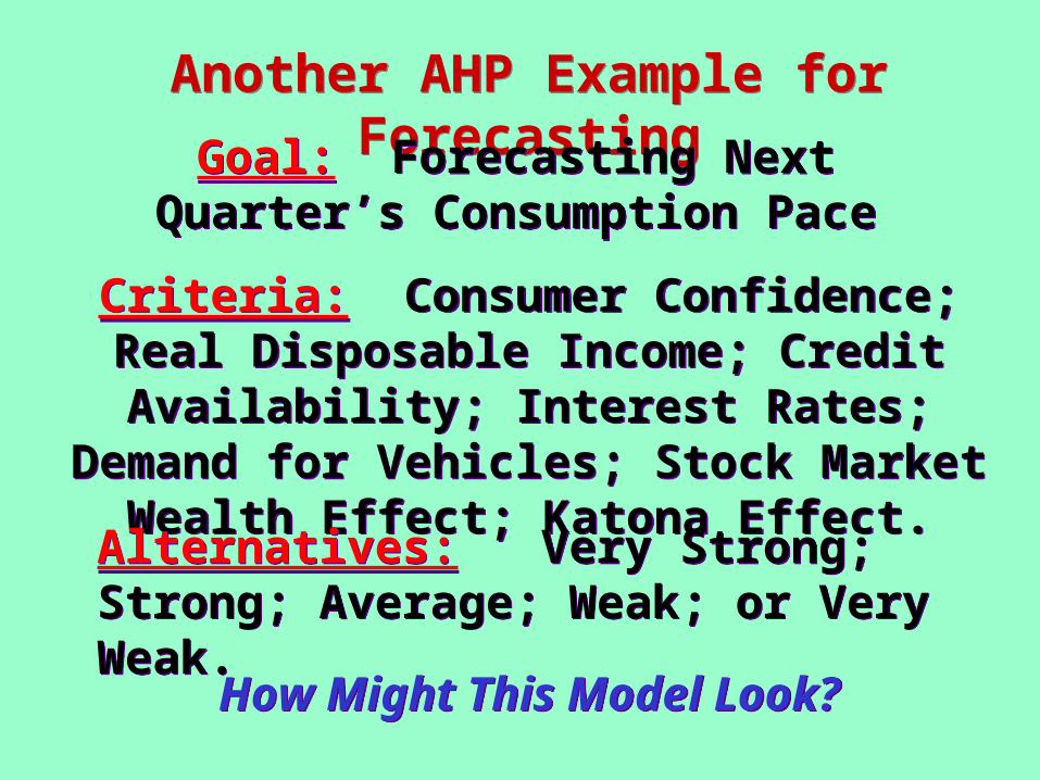
Question: How do you interpret the cells in the matrix?
Answer: While it may seem strange to compare, say, the “Very Strong” to the “Weak” criterion, this is precisely
what Saaty did in his forecasting application for real growth, which we discussed earlier. But the question that
you should ask is, “which outcome is more likely?”
Fac
tor
Fac
tor
Factor Impact on ObjectiveFactor Impact on Objective
Q&A about Pairwise Comparisons
VS S M W VW Very Strong (VS) 1.0 1/AA 1/BB 1/CC 1/DD Strong (S) AA 1.0 1/GG 1/HH 1/II Moderate (M) BB GG 1.0 1/LL 1/MM Weak (W) CC HH LL 1.0 1/PP Very Weak (VW) DD II MM PP 1.0
VS S M W VW Very Strong (VS) 1.0 1/AA 1/BB 1/CC 1/DD Strong (S) AA 1.0 1/GG 1/HH 1/II Moderate (M) BB GG 1.0 1/LL 1/MM Weak (W) CC HH LL 1.0 1/PP Very Weak (VW) DD II MM PP 1.0
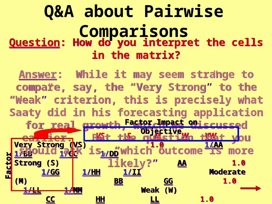
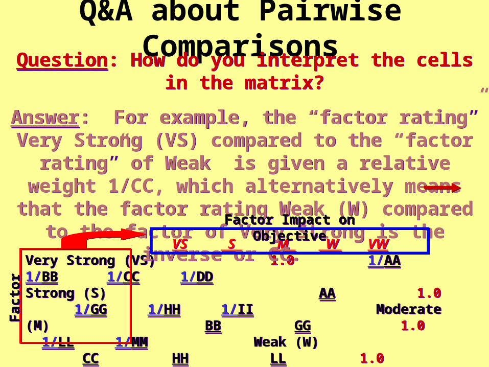
Question: How do you interpret the cells in the matrix?
Answer: For example, the “factor rating” Very Strong (VS) compared to the “factor rating” of Weak is given a relative weight 1/CC, which alternatively means that the factor rating Weak (W) compared to the factor of Very
Strong is the inverse or CC.
Fac
tor
Fac
tor
Factor Impact on ObjectiveFactor Impact on Objective

Q&A about Pairwise Comparisons
VS S M W VW Very Strong (VS) 1.0 1/AA 1/BB 1/CC 1/DD Strong (S) AA 1.0 1/GG 1/HH 1/II Moderate (M) BB GG 1.0 1/LL 1/MM Weak (W) CC HH LL 1.0 1/PP Very Weak (VW) DD II MM PP 1.0
VS S M W VW Very Strong (VS) 1.0 1/AA 1/BB 1/CC 1/DD Strong (S) AA 1.0 1/GG 1/HH 1/II Moderate (M) BB GG 1.0 1/LL 1/MM Weak (W) CC HH LL 1.0 1/PP Very Weak (VW) DD II MM PP 1.0
Question: How do you interpret the cells in the matrix?
Answer: So, for example, if you think that the factor intensity is “Strong” (5) for, say income, relative to its
impact on consumption and the factor rating for “weak” income is 2, then the cell entry is “5/2”. Do not confuse the rating scale with the magnitude categories in the forecast
objective.
Fac
tor
Fac
tor
Factor Impact on ObjectiveFactor Impact on Objective

Q&A about Pairwise Comparisons
VS S M W VW Very Strong (VS) 1.0 1/AA 1/BB 1/CC 1/DD Strong (S) AA 1.0 1/GG 1/HH 1/II Moderate (M) BB GG 1.0 1/LL 1/MM Weak (W) CC HH LL 1.0 1/PP Very Weak (VW) DD II MM PP 1.0
VS S M W VW Very Strong (VS) 1.0 1/AA 1/BB 1/CC 1/DD Strong (S) AA 1.0 1/GG 1/HH 1/II Moderate (M) BB GG 1.0 1/LL 1/MM Weak (W) CC HH LL 1.0 1/PP Very Weak (VW) DD II MM PP 1.0
Question: How do you interpret the cells in the matrix?
Answer: Therefore, pairwise-comparison cell (VS,W) or 1/CC is 5/2. Alternatively, the cell (W, VS), which is CC is
2/5, which simply suggests that a very strong gain in income will have a larger impact of strong consumption
than a weak income gain.
Fac
tor
Fac
tor
Factor Impact on ObjectiveFactor Impact on Objective

Q&A about Pairwise Comparisons
VS S M W VW Very Strong (VS) 1.0 1/AA 1/BB 1/CC 1/DD Strong (S) AA 1.0 1/GG 1/HH 1/II Moderate (M) BB GG 1.0 1/LL 1/MM Weak (W) CC HH LL 1.0 1/PP Very Weak (VW) DD II MM PP 1.0
VS S M W VW Very Strong (VS) 1.0 1/AA 1/BB 1/CC 1/DD Strong (S) AA 1.0 1/GG 1/HH 1/II Moderate (M) BB GG 1.0 1/LL 1/MM Weak (W) CC HH LL 1.0 1/PP Very Weak (VW) DD II MM PP 1.0
Question: How do you interpret the cells in the matrix?
Answer: The numbers in the Saaty scale are independent of the measurement units used. If you enter 2, you mean the larger factor has two times the impact as the smaller
factor.
Question: How do you interpret the cells in the matrix?
Answer: The numbers in the Saaty scale are independent of the measurement units used. If you enter 2, you mean the larger factor has two times the impact as the smaller
factor.
Fac
tor
Fac
tor
Factor Impact on ObjectiveFactor Impact on Objective

Q&A about Pairwise ComparisonsQuestion: What if we believe that all choices in the
matrix should have the same impact on the objective?
Answer: That’s fine and the matrix can be collapsed.
Question: What if we believe that all choices in the matrix should have the same impact on the objective?
Answer: That’s fine and the matrix can be collapsed.
VS S M W VW WEIGHT Very Strong (VS) 1.0 1/1 1/1 1/1 1/1 = 0.20 Strong (S) 1 1.0 1/1 1/1 1/1 = 0.20 Moderate (M) 1 1 1.0 1/1 1/1
= 0.20Weak (W) 1 1 1 1.0 1/1 = 0.20 Very Weak (VW) 1 1 1 1 1.0 = 0.20
VS S M W VW WEIGHT Very Strong (VS) 1.0 1/1 1/1 1/1 1/1 = 0.20 Strong (S) 1 1.0 1/1 1/1 1/1 = 0.20 Moderate (M) 1 1 1.0 1/1 1/1
= 0.20Weak (W) 1 1 1 1.0 1/1 = 0.20 Very Weak (VW) 1 1 1 1 1.0 = 0.20
Fac
tor
Fac
tor
Factor Impact on ObjectiveFactor Impact on Objective
Example Where the Evaluation of the Factor Intensity is 1 for all comparisons.
Example Where the Evaluation of the Factor Intensity is 1 for all comparisons.

Q&A about Pairwise ComparisonsQuestion: What if a factor that typically has a positive impact on the objective will be a negative factor during
the horizon of the problem?
Answer: That should be reflected in the weights. For example, if income is declining, then you might give it a
strong weight for a “weak” reading.
Question: What if a factor that typically has a positive impact on the objective will be a negative factor during
the horizon of the problem?
Answer: That should be reflected in the weights. For example, if income is declining, then you might give it a
strong weight for a “weak” reading.

Example for Determining Weights for Declining Income on Consumption
Example for Determining Weights for Declining Income on Consumption

Q&A about Pairwise ComparisonsQuestion: What if you want an absolute scale instead of
this relative comparison?
Answer: There are various techniques that you can use to develop a quantitative scale. Here is one (known as
the Holmes Method): Calculate the correlation (or R2 is better) between a very strong change in the factor (such as, income) with a very strong change in consumption.
Then do the same for a strong change change in the factor with a very strong change in consumption. Use
those correlation coefficients to assess the absolute impact. Be careful of timing (leads and lags)
relationships.
Question: What if you want an absolute scale instead of this relative comparison?
Answer: There are various techniques that you can use to develop a quantitative scale. Here is one (known as
the Holmes Method): Calculate the correlation (or R2 is better) between a very strong change in the factor (such as, income) with a very strong change in consumption.
Then do the same for a strong change change in the factor with a very strong change in consumption. Use
those correlation coefficients to assess the absolute impact. Be careful of timing (leads and lags)
relationships.

Q&A about Pairwise ComparisonsAnswer (Continued): Although this is tedious, EVIEWS can do this easily with a conditional statement. You can
also do that in EXCEL, but you must calculate the correlation only using values that meet the condition -- say, real consumption growth greater than 4.5% and
real disposable income growth greater than 6.6%(geometric mean plus 1 deviation, 1989-99) -- VERY STRONG INCOME GROWTH vs. VERY STRONG
CONSUMPTION GROWTH. Similarly that would be done for STRONG INCOME GROWTH (geometric mean plus .25* deviation, which is 4.1%, to 6.5%) vs.
VERY STRONG CONSUMPTION GROWTH and so on.
Answer (Continued): Although this is tedious, EVIEWS can do this easily with a conditional statement. You can
also do that in EXCEL, but you must calculate the correlation only using values that meet the condition -- say, real consumption growth greater than 4.5% and
real disposable income growth greater than 6.6%(geometric mean plus 1 deviation, 1989-99) -- VERY STRONG INCOME GROWTH vs. VERY STRONG
CONSUMPTION GROWTH. Similarly that would be done for STRONG INCOME GROWTH (geometric mean plus .25* deviation, which is 4.1%, to 6.5%) vs.
VERY STRONG CONSUMPTION GROWTH and so on.

Setup Matrix of Lower Pairwise Comparisons
VS S M W VW Very Strong (VS) 1.0 1/AA 1/BB 1/CC 1/DD Strong (S) AA 1.0 1/GG 1/HH 1/II Moderate (M) BB GG 1.0 1/LL 1/MM Weak (W) CC HH LL 1.0 1/PP Very Weak (VW) DD II MM PP 1.0
VS S M W VW Very Strong (VS) 1.0 1/AA 1/BB 1/CC 1/DD Strong (S) AA 1.0 1/GG 1/HH 1/II Moderate (M) BB GG 1.0 1/LL 1/MM Weak (W) CC HH LL 1.0 1/PP Very Weak (VW) DD II MM PP 1.0
Question: How Much Impact Does Consumer Confidence Have on Real Consumer Spending
Growth?
Question: How Much Impact Does Consumer Confidence Have on Real Consumer Spending
Growth?
This must be filled in for every alternative . . .This must be filled in for every alternative . . .

Finally, collect the individual equations into a spreadsheet.
Finally, collect the individual equations into a spreadsheet.

Determine the Final Forecast Based on Mid-Point Range Estimates (or Some other
Criteria).
Determine the Final Forecast Based on Mid-Point Range Estimates (or Some other
Criteria).
ImpactWeights
Net Impact
See Next Slide for Additional BreakoutSee Next Slide for Additional Breakout
Consumer Spending Forecast =
3.0%
Consumer Spending Forecast =
3.0%

Partial Impact of Confidence on Consumer Spending.
Partial Impact of Confidence on Consumer Spending.
Consumer Spending IMPACT from CC = .031*CC
CC = 0.351*VS+0.173*S+0.106*M+0.150*W+0.220*VW
Consumer Spending IMPACT from CC = .031*CC
CC = 0.351*VS+0.173*S+0.106*M+0.150*W+0.220*VW

Limitations of AHPLimitations of AHP
1. Unicausal Modeling Only. It Does Not Incorporate Feedback Effects.
It Assumes the “Criteria” are Relatively Independent over the
Time Frame Forecasted.
2. Difficult or Impossible to Check Historical Accuracy.
1. Unicausal Modeling Only. It Does Not Incorporate Feedback Effects.
It Assumes the “Criteria” are Relatively Independent over the
Time Frame Forecasted.
2. Difficult or Impossible to Check Historical Accuracy.

Some Extensions of AHPSome Extensions of AHPNetwork Modeling with Feedback
Analytic Network Process (ANP)
Network Modeling with Feedback
Analytic Network Process (ANP)

Fast-Food Retail Industry ANP Model
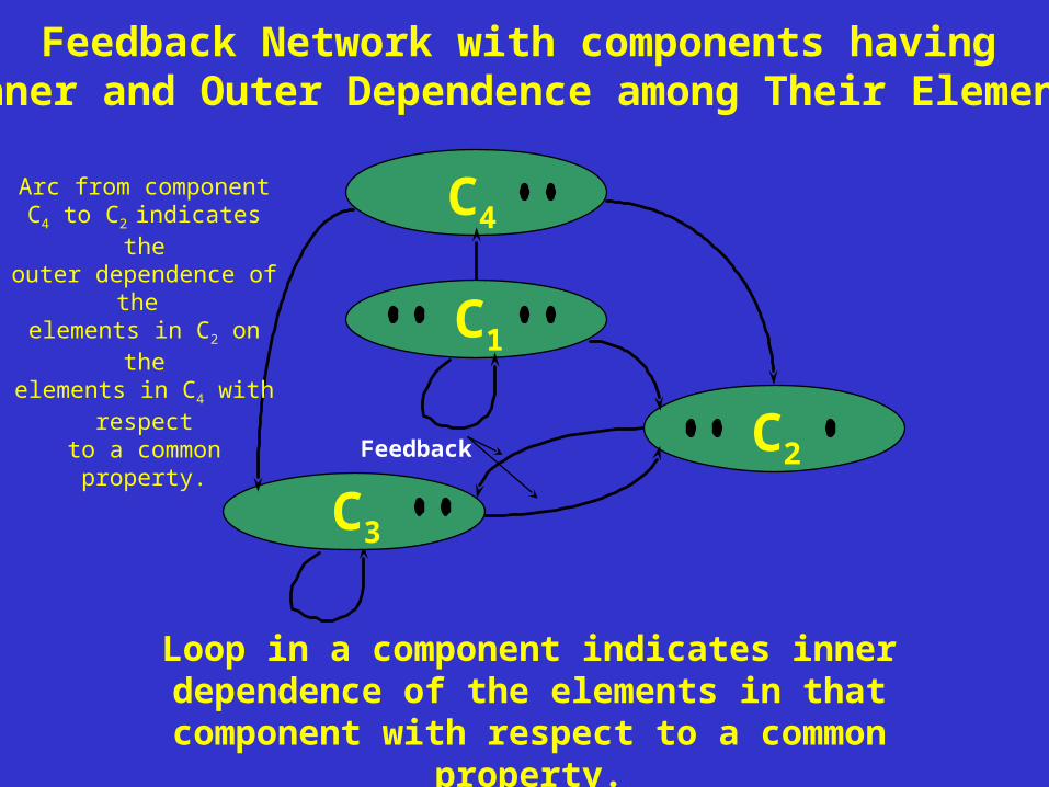
Feedback Network with components having Inner and Outer Dependence among Their Elements
C4
C1
C2
C3
Feedback
Loop in a component indicates inner dependence of the elements in that component with respect to a
common property.
Arc from componentC4 to C2 indicates the
outer dependence of the elements in C2 on theelements in C4 with
respectto a common property.

Cluster Weights 1. Competition 2. Adverrtising 3. Quality 4. Other1. Competition 0.2146 0.2470 0.5000 0.18702. Adverrtising 0.5328 0.6223 0.0000 0.13073. Quality 0.0656 0.0000 0.0000 0.50004. Other 0.1870 0.1307 0.5000 0.1984
Fast-Food Retail Industry Model
Priority Weightings

Burger King White Collar Blue Collar Student Family PrioritiesWhite collar 1 4 5 1 / 3 0.299Blue collar 1 / 4 1 4 1 / 3 0.138Student 1 / 5 1 / 4 1 1/ 7 0.051Family 3 3 7 1 0.512
Pairwise Judgments of the Customer Group for Burger King

Local: Menu Cleanliness
Speed Service Location Price Reputation
TakeOut
Portion Taste Nutrition
Frequency
Promotion
Creativity
Wendy’s BurgerKing
McDon-ald’s
Menu Item 0.0000 0.0000 0.0000 0.0000 0.0000 0.0000 0.1930 0.0000 0.0000 0.0000 0.0000 0.3110 0.1670 0.1350 0.1570 0.0510 0.1590Cleanliness 0.6370 0.0000 0.0000 0.5190 0.0000 0.0000 0.2390 0.0000 0.0000 0.0000 0.0000 0.0000 0.0000 0.0000 0.2760 0.1100 0.3330Speed 0.1940 0.7500 0.0000 0.2850 0.0000 0.0000 0.0830 0.2900 0.0000 0.0000 0.0000 0.0000 0.0000 0.0000 0.0640 0.1400 0.0480Service 0.0000 0.0780 0.1880 0.0000 0.0000 0.0000 0.0450 0.0550 0.0000 0.0000 0.0000 0.0000 0.0000 0.0000 0.0650 0.1430 0.0240Location 0.0530 0.1710 0.0000 0.0980 0.0000 0.5000 0.2640 0.6550 0.0000 0.0000 0.0000 0.1960 0.0000 0.7100 0.1420 0.2240 0.1070Price 0.1170 0.0000 0.0000 0.0000 0.0000 0.0000 0.0620 0.0000 0.8570 0.0000 0.0000 0.0000 0.8330 0.0000 0.0300 0.2390 0.0330Reputation 0.0000 0.0000 0.0810 0.0980 0.0000 0.0000 0.0570 0.0000 0.0000 0.0000 0.0000 0.4930 0.0000 0.1550 0.2070 0.0420 0.2230Take-Out 0.0000 0.0000 0.7310 0.0000 0.0000 0.5000 0.0570 0.0000 0.1430 0.0000 0.0000 0.0000 0.0000 0.0000 0.0590 0.0510 0.0740Portion 0.2290 0.0000 0.0000 0.0000 0.0000 0.8330 0.2800 0.0000 0.0000 0.0000 0.0000 0.0000 0.0000 0.0000 0.0940 0.6490 0.5280Taste 0.6960 0.0000 0.0000 0.0000 0.0000 0.0000 0.6270 0.0000 0.0000 0.0000 0.0000 0.0000 0.0000 0.0000 0.2800 0.0720 0.1400Nutrition 0.0750 0.0000 0.0000 0.0000 0.0000 0.1670 0.0940 0.0000 0.0000 0.0000 0.0000 0.0000 0.0000 0.0000 0.6270 0.2790 0.3320Frequency 0.7500 0.0000 0.0000 0.0000 0.0000 0.1670 0.5500 0.0000 0.0000 0.0000 0.0000 0.0000 0.6670 0.8750 0.6490 0.7090 0.6610Promotion 0.1710 0.0000 0.0000 0.0000 0.0000 0.8330 0.3680 0.0000 0.0000 0.0000 0.0000 0.5000 0.0000 0.1250 0.0720 0.1130 0.1310Creativity 0.0780 0.0000 0.0000 0.0000 0.0000 0.0000 0.0820 0.0000 0.0000 0.0000 0.0000 0.5000 0.3330 0.0000 0.2790 0.1790 0.2080Wendy's 0.3110 0.5000 0.0990 0.5280 0.0950 0.0950 0.1010 0.1960 0.2760 0.6050 0.5940 0.0880 0.0880 0.1170 0.0000 0.1670 0.2000Burger King 0.1960 0.2500 0.3640 0.1400 0.2500 0.2500 0.2260 0.3110 0.1280 0.1050 0.1570 0.1950 0.1950 0.2680 0.2500 0.0000 0.8000McDonald’s 0.4930 0.2500 0.5370 0.3330 0.6550 0.6550 0.6740 0.4940 0.5950 0.2910 0.2490 0.7170 0.7170 0.6140 0.7500 0.8330 0.0000
Hamburger Model Supermatrix
Cluster: Other Quality Advertising CompetitionOther 0.198 0.500 0.131 0.187Quality 0.066 0.000 0.000 0.066Advertising 0.607 0.000 0.622 0.533Competition 0.129 0.500 0.247 0.215
Cluster Priorities Matrix
Other
Q
AdComp
Other Quality CompetitionAdvertising