Agenda for Week 4 (Tuesday, Jan 26)

Week 4 Hour 1

AnOVa review.

Week 4 Hour 2

Multiple Testing

Tukey’s HSD (Honestly Significant Difference).

Week 4 Hour 3 (Thursday)

Two-way AnOVa.

Sometimes you’ll need to test many hypotheses together.

Example: To check that a new drug doesn’t have side effects, we’d want to test that it doesn’t change…

blood pressure,

hours slept,

heart rate,

levels of various horomones…

Each of these aspects of the body needs its own hypothesis test.

Assume the drug doesn’t have any side effects

If we use α = 0.05 for each of those aspects then there’s

a 5% chance of finding a change in blood pressure, and

a 5% chance of finding a change in hours slept, and

a 5% chance of…

The chance of falsely concluding the drug has side effects is a lot higher than 5% because those chances are all for different things, they stack up.

For testing four things at 5%, we’d reject one falsely 18.54% of the time.

If we wanted the general null hypothesis that the drug has no side effects to have a 5% type 1 error rate, we’d need a

multiple testing correction.

The simplest and most flexible of these corrections (Sidak, Bonferroni, etc.) reduce the alpha for each test until there’s only a 5% chance of even a single false rejection.

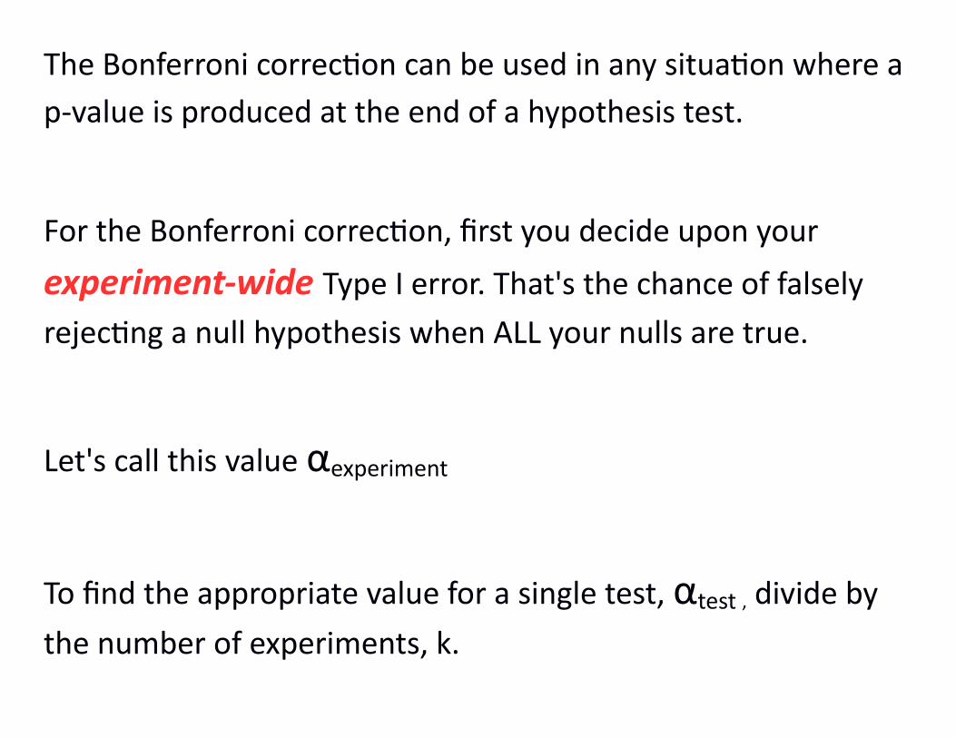
The Bonferroni correction can be used in any situation where a p-value is produced at the end of a hypothesis test.

For the Bonferroni correction, first you decide upon your

experiment-wide Type I error. That's the chance of falsely rejecting a null hypothesis when ALL your nulls are true.

Let's call this value αexperiment

To find the appropriate value for a single test, αtest , divide by the number of experiments, k.

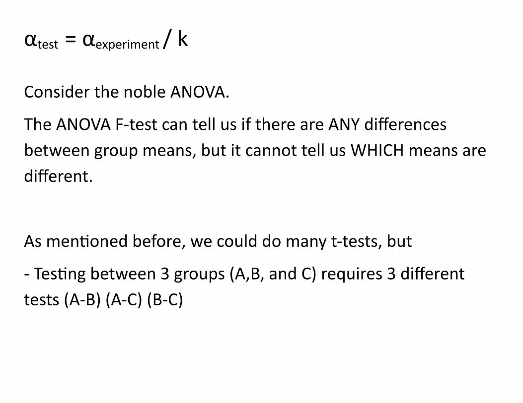
αtest = αexperiment / k

Consider the noble ANOVA.

The ANOVA F-test can tell us if there are ANY differences between group means, but it cannot tell us WHICH means are different.

As mentioned before, we could do many t-tests, but

- Testing between 3 groups (A,B, and C) requires 3 different tests (A-B) (A-C) (B-C)

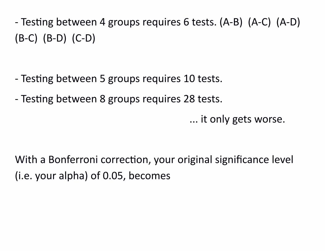
- Testing between 4 groups requires 6 tests. (A-B) (A-C) (A-D) (B-C) (B-D) (C-D)

- Testing between 5 groups requires 10 tests.

- Testing between 8 groups requires 28 tests.

... it only gets worse.

With a Bonferroni correction, your original significance level (i.e. your alpha) of 0.05, becomes

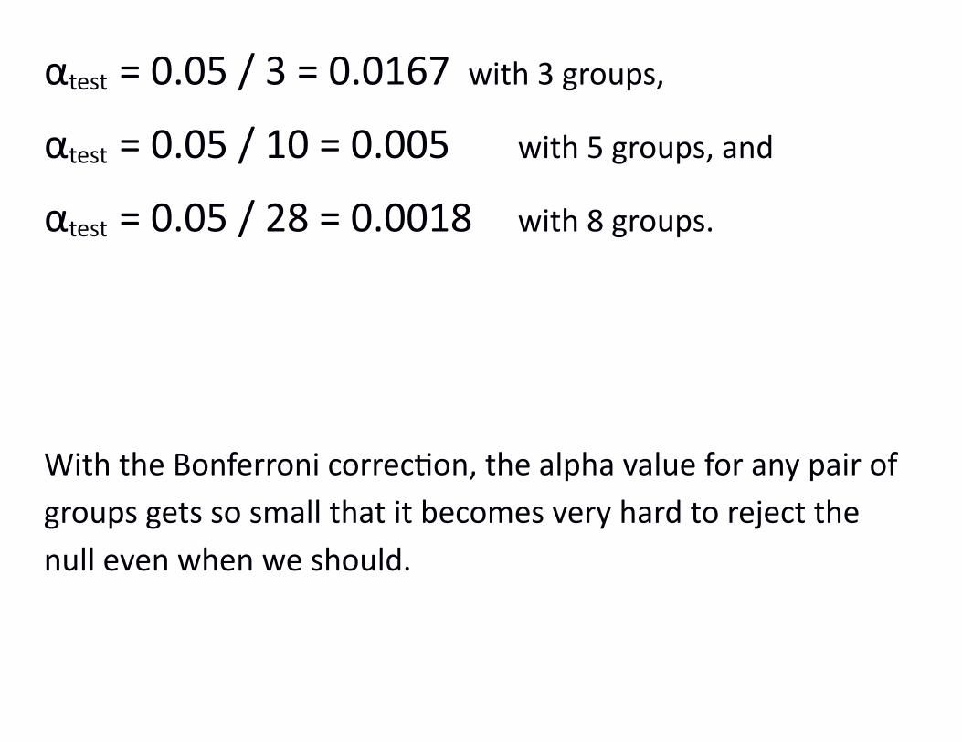
αtest = 0.05 / 3 = 0.0167 with 3 groups,

αtest = 0.05 / 10 = 0.005 with 5 groups, and

αtest = 0.05 / 28 = 0.0018 with 8 groups.

With the Bonferroni correction, the alpha value for any pair of groups gets so small that it becomes very hard to reject the null even when we should.

In other words, it reduces our power too much.

To recap:

- Multiple hypothesis testing has a problem: The chance of a Type I error accumulates.

- Trying to do the t-tests to get more detailed information from an ANOVA involves multiple testing, especially when there are many groups.

- Bonferroni is a simple and flexible way to deal with multiple testing issues, but it causes loss of power.

So how do we maintain power?

Tukey's HSD

John Tukey made a system for managing multiple comparisons in ANOVA that still keeps the experiment-wide error at or below set significance level (e.g. 0.05) without maintaining as much power as possible.

His motivation was the way that researchers were applying t-tests to group differences for 3 or more groups, which he called'scientifically dishonest'

Hence he found the HSD, or Honestly Significant Differences.

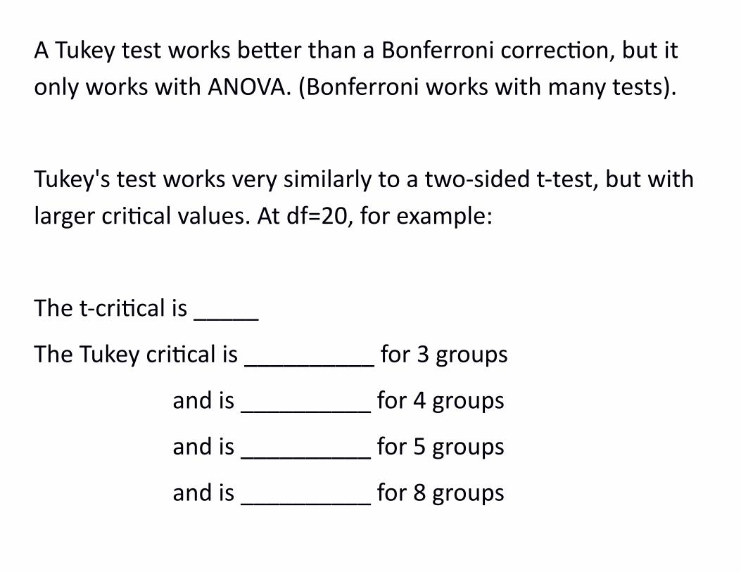
A Tukey test works better than a Bonferroni correction, but it only works with ANOVA. (Bonferroni works with many tests).

Tukey's test works very similarly to a two-sided t-test, but with larger critical values. At df=20, for example:

The t-critical is _____

The Tukey critical is __________ for 3 groups

and is __________ for 4 groups

and is __________ for 5 groups

and is __________ for 8 groups

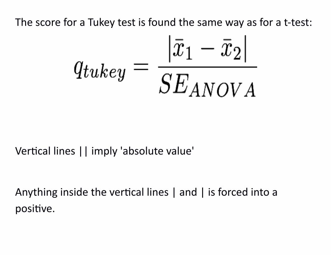
The score for a Tukey test is found the same way as for a t-test:

Vertical lines || imply 'absolute value'

Anything inside the vertical lines | and | is forced into a positive.

Since only the positive side is considered, any Tukey tests are one-sided.

In a t-test, the standard error of the difference (SEdiff), is calculated using information from only two groups.

However, we have more than two groups, but we also have a value from the ANOVA table we can use: MSresid, or MSE.

We will call the standard error of a group mean SEANOVA to emphasize that it comes from the ANOVA information.

MSresid is the variance of the values in any given group.*

The standard error of a mean is sqrt(variance / n),

where n is the size of the group. (Or the smallest group)

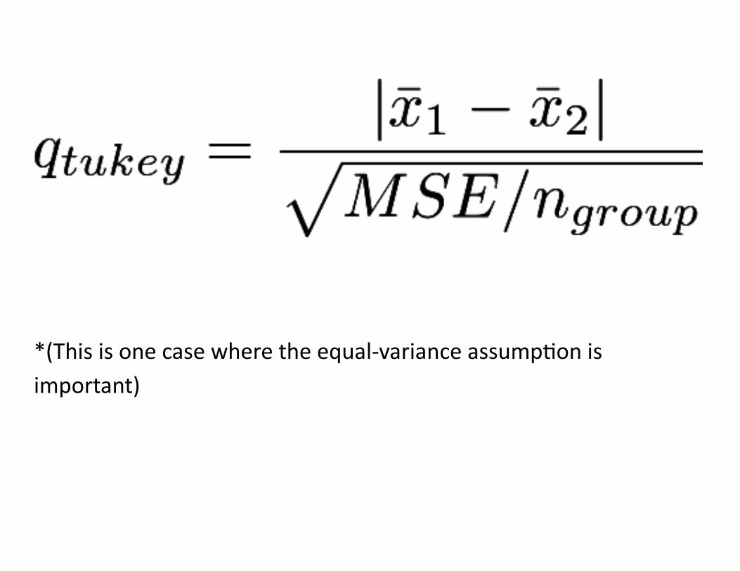
*(This is one case where the equal-variance assumption is important)

Tukey:

More than just a turkey and a toucan.

A Tukey test involves four steps.

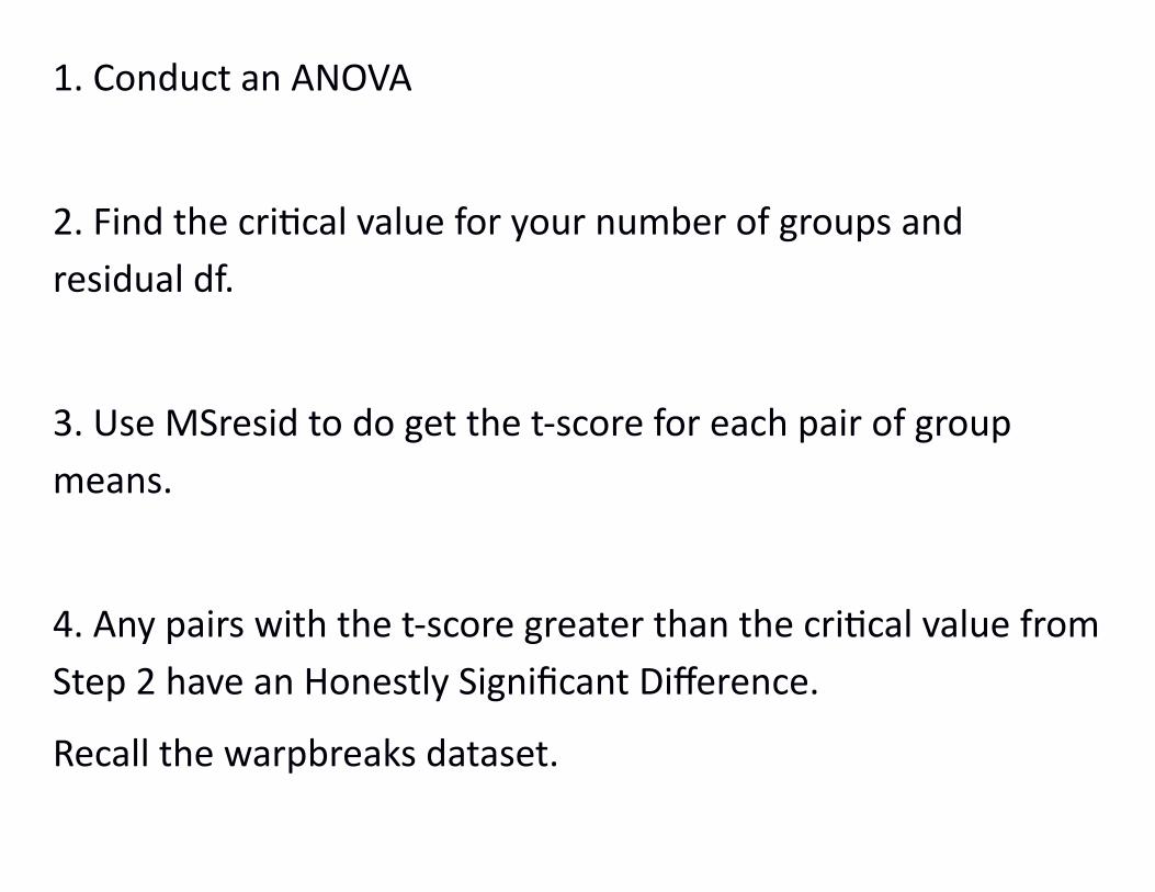
1. Conduct an ANOVA

2. Find the critical value for your number of groups and residual df.

3. Use MSresid to do get the t-score for each pair of group means.

4. Any pairs with the t-score greater than the critical value fromStep 2 have an Honestly Significant Difference.

Recall the warpbreaks dataset.

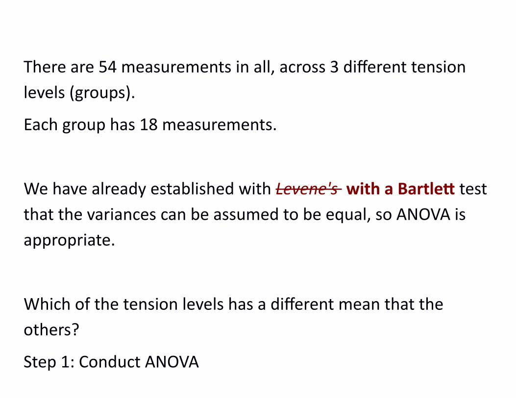
There are 54 measurements in all, across 3 different tension levels (groups).

Each group has 18 measurements.

We have already established with Levene's with a Bartlett test that the variances can be assumed to be equal, so ANOVA is appropriate.

Which of the tension levels has a different mean that the others?

Step 1: Conduct ANOVA

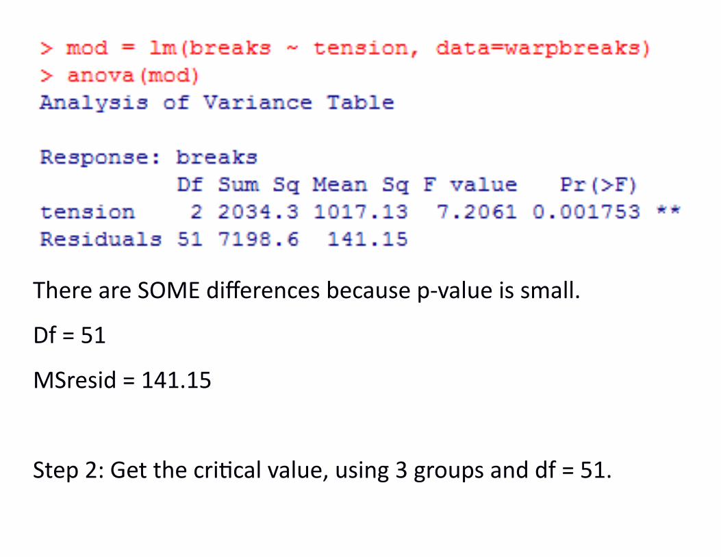
There are SOME differences because p-value is small.

Df = 51

MSresid = 141.15

Step 2: Get the critical value, using 3 groups and df = 51.

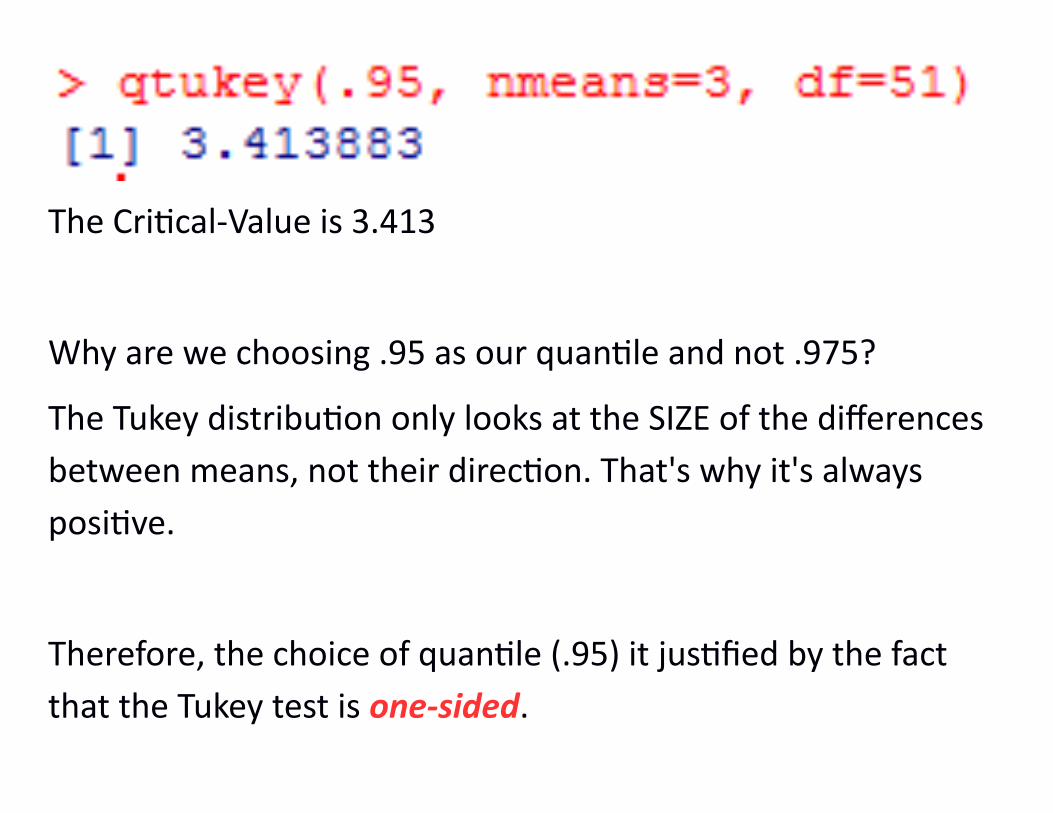
The Critical-Value is 3.413

Why are we choosing .95 as our quantile and not .975?

The Tukey distribution only looks at the SIZE of the differences between means, not their direction. That's why it's always positive.

Therefore, the choice of quantile (.95) it justified by the fact that the Tukey test is one-sided.

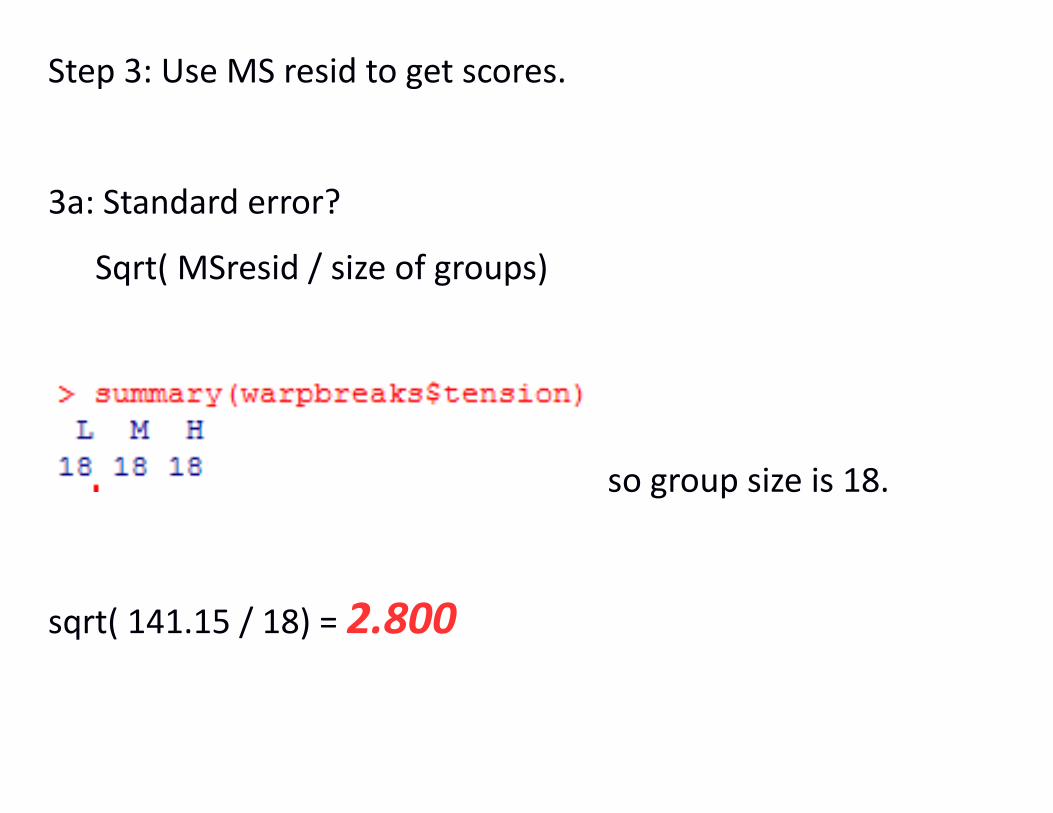
Step 3: Use MS resid to get scores.

3a: Standard error?

Sqrt( MSresid / size of groups)

so group size is 18.

sqrt( 141.15 / 18) = 2.800

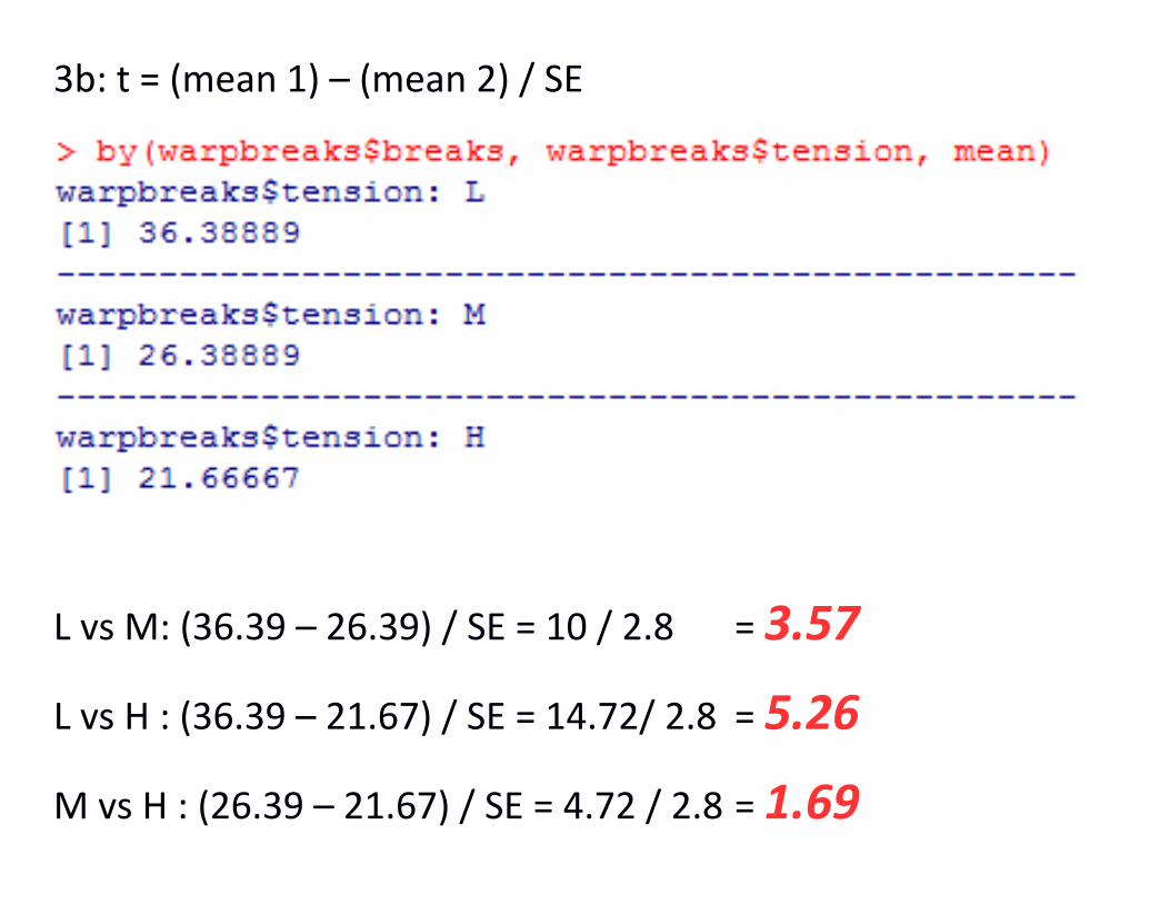
3b: t = (mean 1) – (mean 2) / SE

L vs M: (36.39 – 26.39) / SE = 10 / 2.8 = 3.57

L vs H : (36.39 – 21.67) / SE = 14.72/ 2.8 = 5.26

M vs H : (26.39 – 21.67) / SE = 4.72 / 2.8 = 1.69

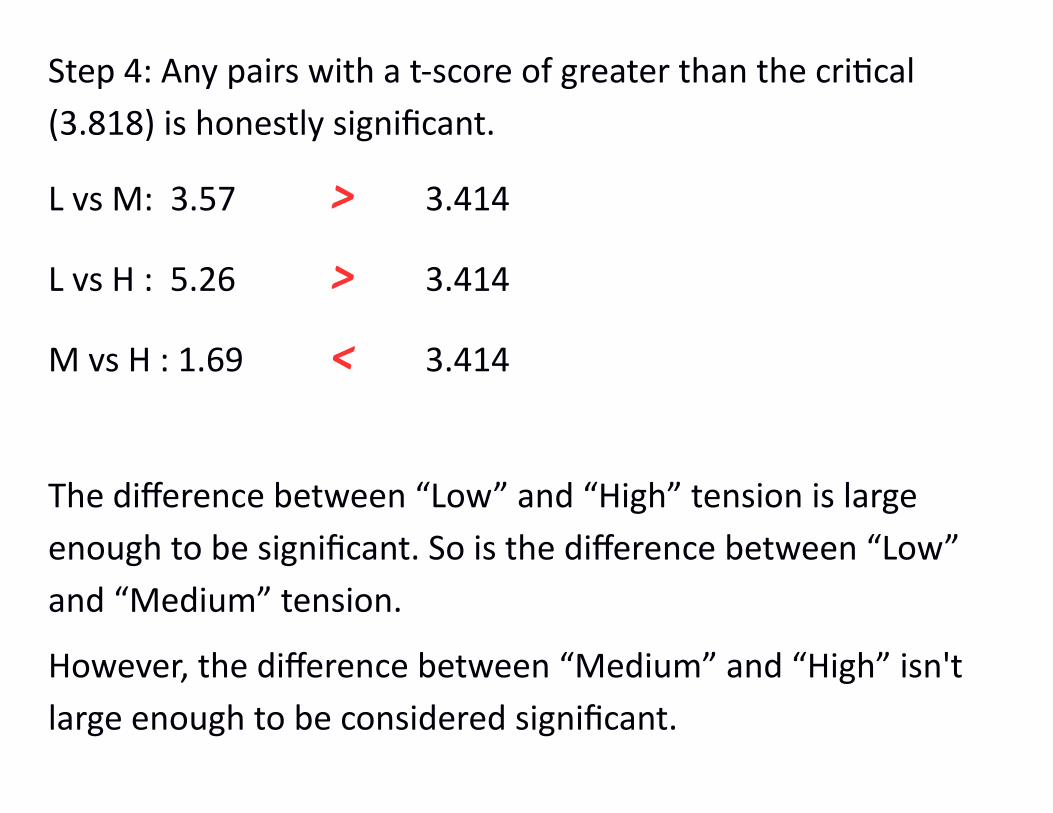
Step 4: Any pairs with a t-score of greater than the critical (3.818) is honestly significant.

L vs M: 3.57 > 3.414

L vs H : 5.26 > 3.414

M vs H : 1.69 < 3.414

The difference between “Low” and “High” tension is large enough to be significant. So is the difference between “Low” and “Medium” tension.

However, the difference between “Medium” and “High” isn't large enough to be considered significant.

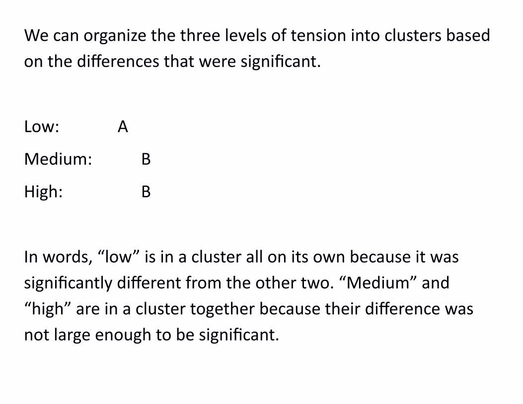
We can organize the three levels of tension into clusters based on the differences that were significant.

Low: A

Medium: B

High: B

In words, “low” is in a cluster all on its own because it was significantly different from the other two. “Medium” and “high” are in a cluster together because their difference was not large enough to be significant.

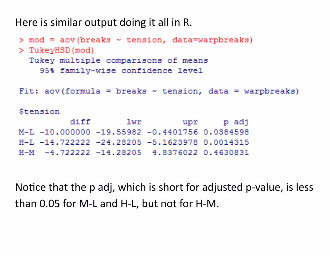
Here is similar output doing it all in R.

Notice that the p adj, which is short for adjusted p-value, is lessthan 0.05 for M-L and H-L, but not for H-M.