Embed Size (px)
Citation preview
Anshul Kumar, CSE IITD
CSL718 : Pipelined ProcessorsCSL718 : Pipelined ProcessorsCSL718 : Pipelined ProcessorsCSL718 : Pipelined Processors
PipelineTimings
12th Jan, 2006
Anshul Kumar, CSE IITD slide 2
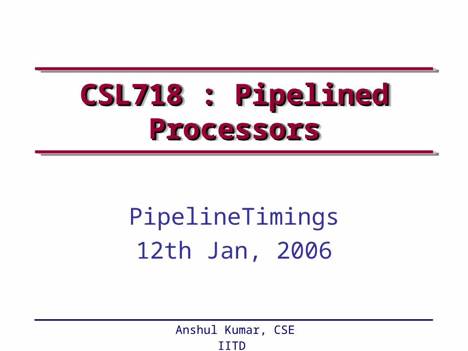
Pipelined ProcessorsPipelined ProcessorsPipelined ProcessorsPipelined Processors
Function-parallel
Instr level (ILP) Thread level Process level
Pipelined processors
VLIWs Superscalar processors
Parallel architectures
Data-parallel
Intel’s terminology:
• intra ILP
• inter ILP
Anshul Kumar, CSE IITD slide 3
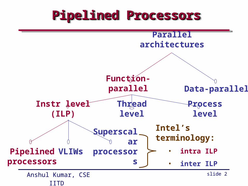
Processor PerformanceProcessor PerformanceProcessor PerformanceProcessor Performance
• MIPS and MFLOPS
may not truly represent performance
• Execution time of a program
true measure of performance
• SPEC rating
acceptable
Anshul Kumar, CSE IITD slide 4
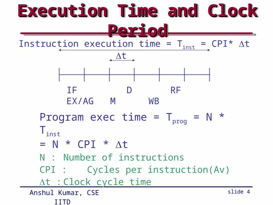
Execution Time and Clock PeriodExecution Time and Clock PeriodExecution Time and Clock PeriodExecution Time and Clock Period
Program exec time = Tprog = N * Tinst
= N * CPI * tN : Number of instructionsCPI : Cycles per instruction(Av)t : Clock cycle time
IF D RF EX/AG M WB
Instruction execution time = Tinst = CPI* tt
Anshul Kumar, CSE IITD slide 5
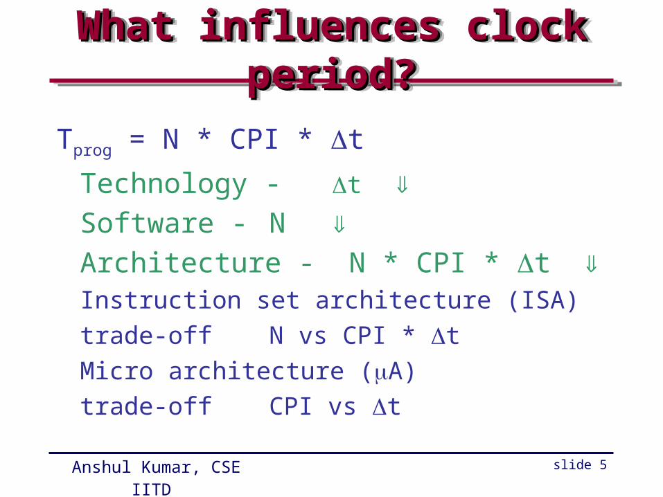
What influences clock period?What influences clock period?What influences clock period?What influences clock period?
Tprog = N * CPI * t
Technology - t
Software - N
Architecture - N * CPI * t Instruction set architecture (ISA)
trade-off N vs CPI * t
Micro architecture (A)
trade-off CPI vs t
Anshul Kumar, CSE IITD slide 6
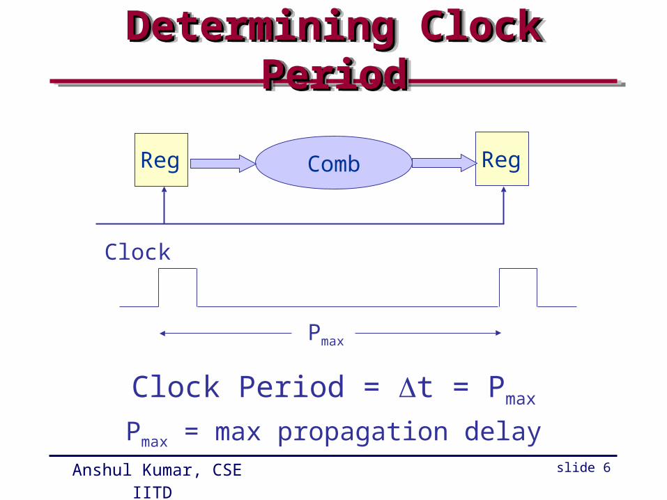
Determining Clock PeriodDetermining Clock PeriodDetermining Clock PeriodDetermining Clock Period
Clock Period = t = Pmax
Pmax = max propagation delay
Clock
Pmax
CombReg Reg
Anshul Kumar, CSE IITD slide 7
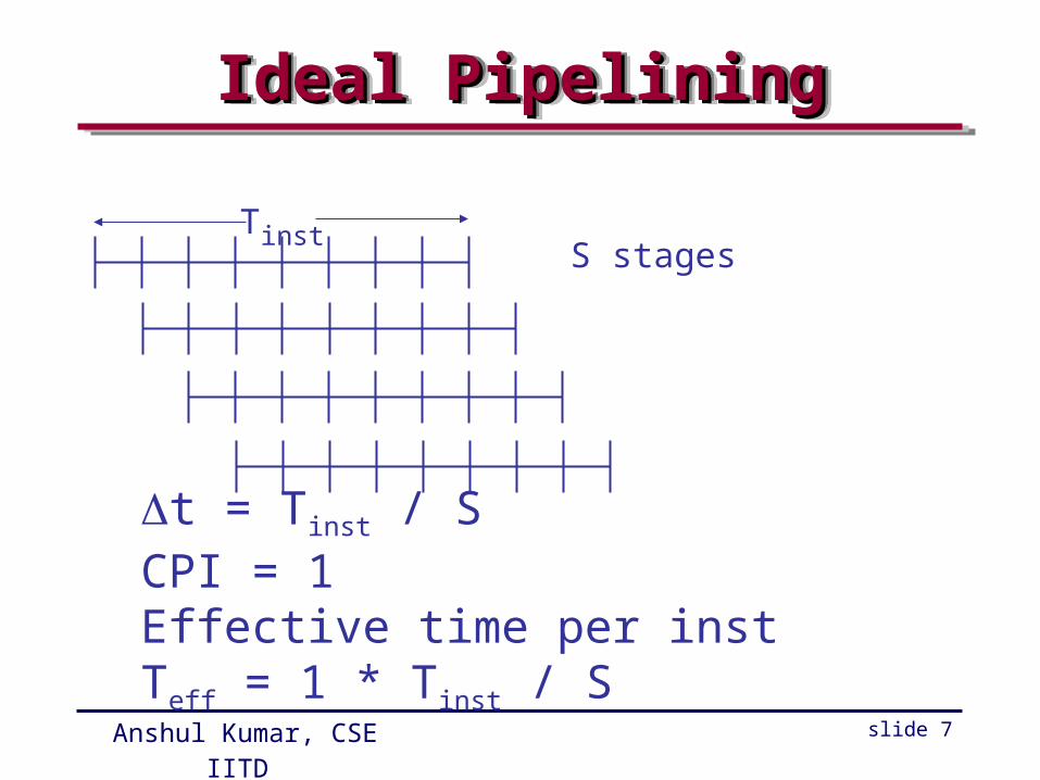
Ideal PipeliningIdeal PipeliningIdeal PipeliningIdeal Pipelining
t = Tinst / SCPI = 1Effective time per inst Teff = 1 * Tinst / S
TinstS stages
Anshul Kumar, CSE IITD slide 8
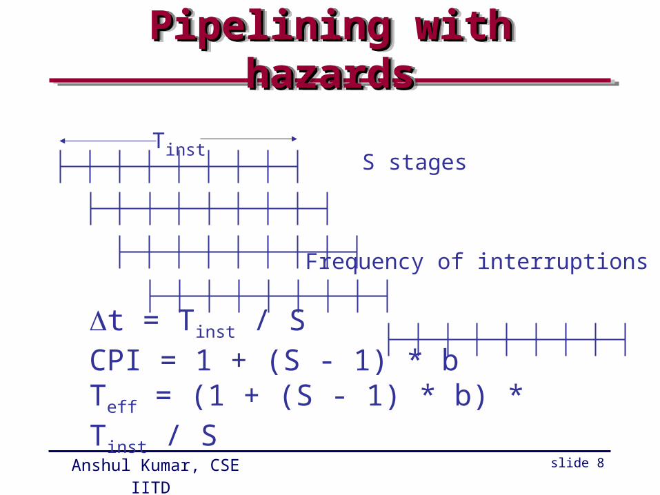
Pipelining with hazardsPipelining with hazardsPipelining with hazardsPipelining with hazards
t = Tinst / SCPI = 1 + (S - 1) * bTeff = (1 + (S - 1) * b) * Tinst / S
TinstS stages
Frequency of interruptions - b
Anshul Kumar, CSE IITD slide 9
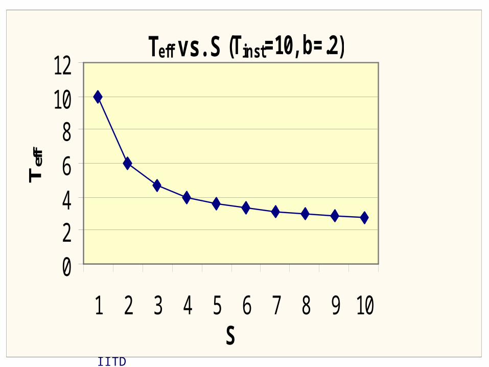
Teff vs. S (Tinst=10, b=.2)
024681012
1 2 3 4 5 6 7 8 9 10S
Tef
f
Anshul Kumar, CSE IITD slide 10
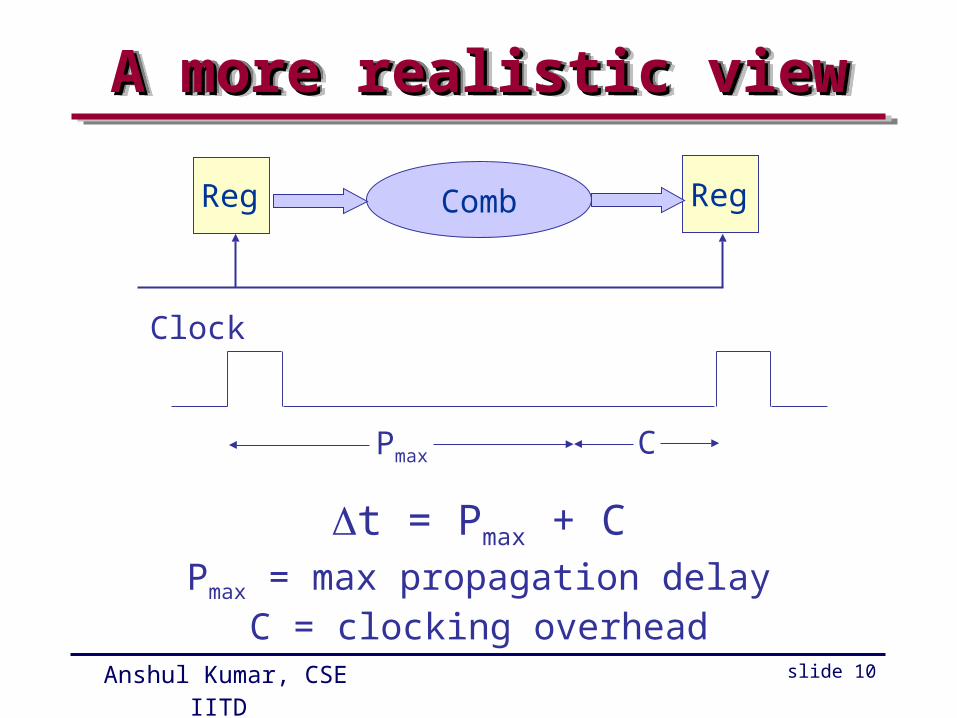
A more realistic viewA more realistic viewA more realistic viewA more realistic view
t = Pmax + CPmax = max propagation delay
C = clocking overhead
Clock
Pmax C
CombReg Reg
Anshul Kumar, CSE IITD slide 11
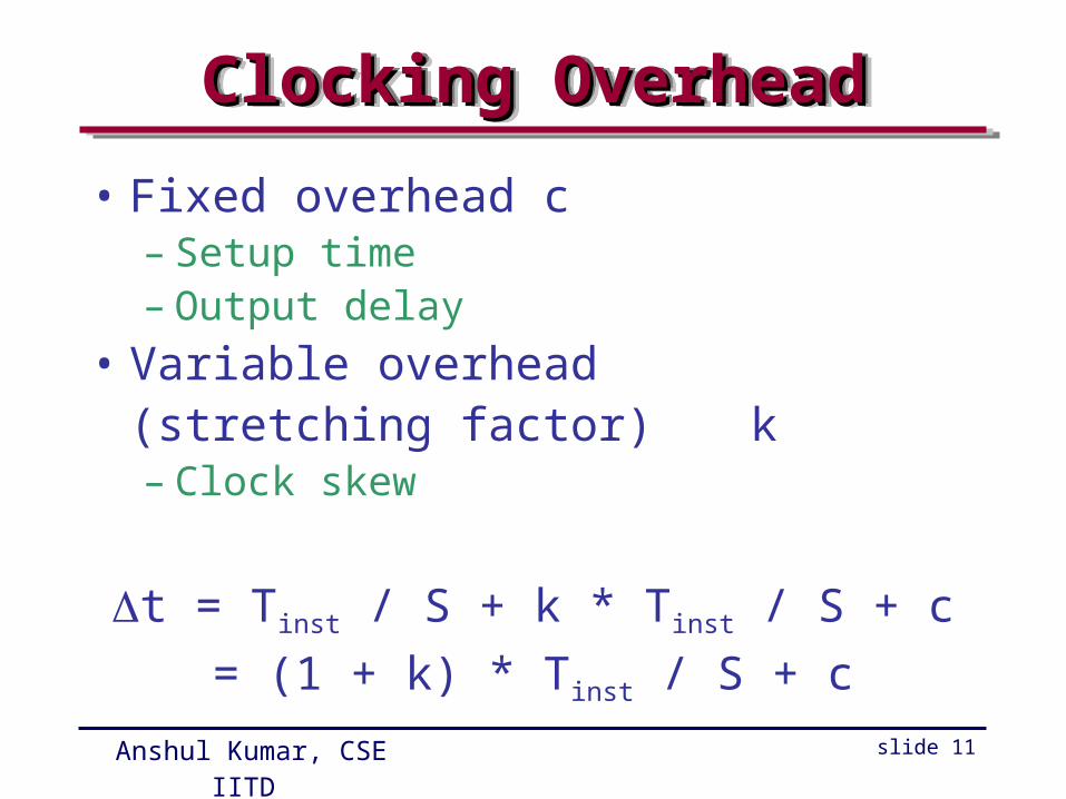
Clocking OverheadClocking OverheadClocking OverheadClocking Overhead
• Fixed overhead c– Setup time – Output delay
• Variable overhead (stretching factor) k
– Clock skew
t = Tinst / S + k * Tinst / S + c
= (1 + k) * Tinst / S + c
Anshul Kumar, CSE IITD slide 12
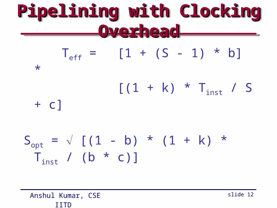
Pipelining with Clocking OverheadPipelining with Clocking OverheadPipelining with Clocking OverheadPipelining with Clocking Overhead
Teff = [1 + (S - 1) * b] *
[(1 + k) * Tinst / S + c]
Sopt = [(1 - b) * (1 + k) * Tinst / (b * c)]
Anshul Kumar, CSE IITD slide 13
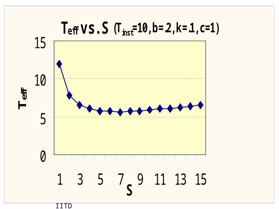
Teff vs. S (Tinst=10, b=.2, k=.1, c=1)
0
5
10
15
1 3 5 7 9 11 13 15S
Tef
f
Anshul Kumar, CSE IITD slide 14
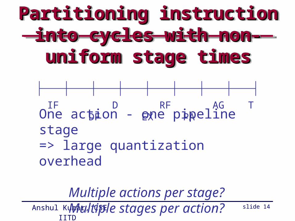
Partitioning instruction into cycles Partitioning instruction into cycles with non-uniform stage timeswith non-uniform stage times
Partitioning instruction into cycles Partitioning instruction into cycles with non-uniform stage timeswith non-uniform stage times
IF D RF AG T DF EX PA
One action - one pipeline stage => large quantization overhead
Multiple actions per stage?Multiple stages per action?
Anshul Kumar, CSE IITD slide 15
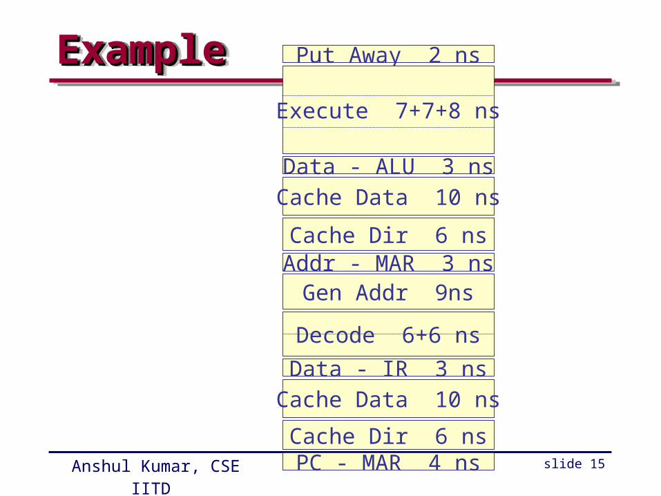
ExampleExampleExampleExample Put Away 2 ns
Data - ALU 3 ns
Addr - MAR 3 ns
Data - IR 3 ns
PC - MAR 4 ns
Cache Dir 6 ns
Cache Dir 6 ns
Cache Data 10 ns
Decode 6+6 ns
Gen Addr 9ns
Cache Data 10 ns
Execute 7+7+8 ns
Anshul Kumar, CSE IITD slide 16
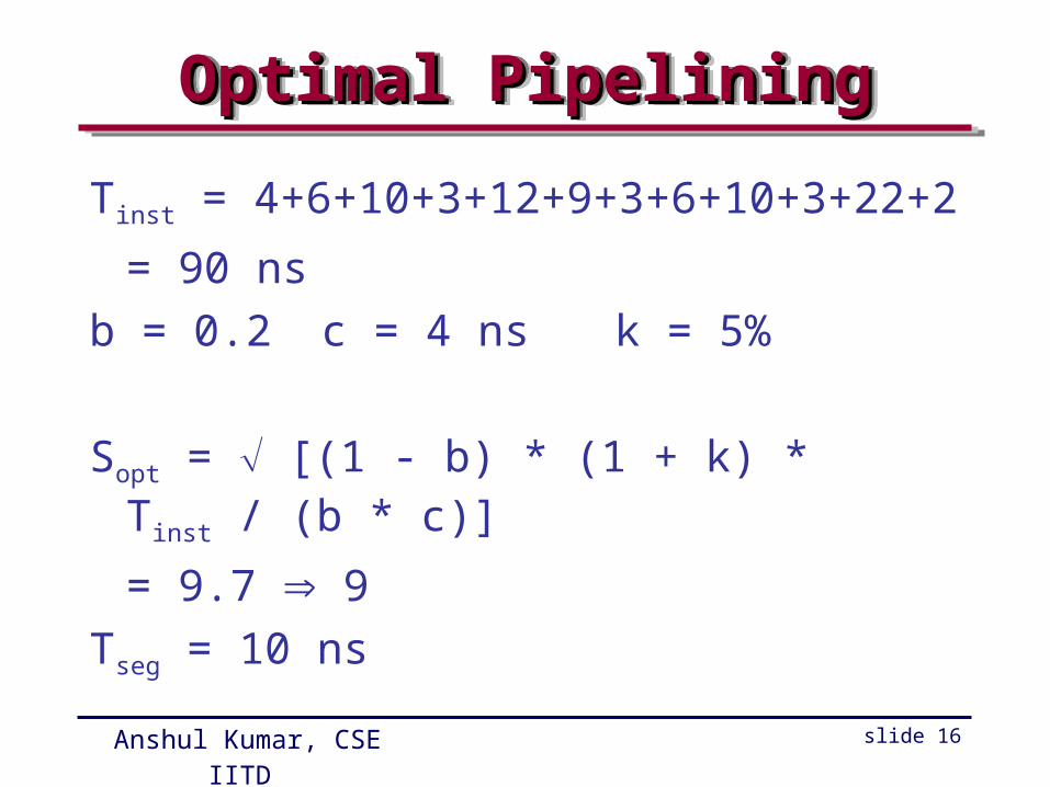
Optimal PipeliningOptimal PipeliningOptimal PipeliningOptimal Pipelining
Tinst = 4+6+10+3+12+9+3+6+10+3+22+2
= 90 ns
b = 0.2 c = 4 ns k = 5%
Sopt = [(1 - b) * (1 + k) * Tinst / (b * c)]
= 9.7 9
Tseg = 10 ns
Anshul Kumar, CSE IITD slide 17
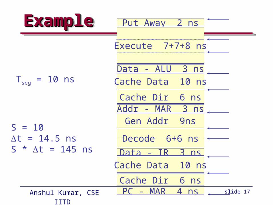
ExampleExampleExampleExample Put Away 2 ns
Data - ALU 3 ns
Addr - MAR 3 ns
Data - IR 3 ns
PC - MAR 4 ns
Cache Dir 6 ns
Cache Dir 6 ns
Cache Data 10 ns
Decode 6+6 ns
Gen Addr 9ns
Cache Data 10 ns
Execute 7+7+8 ns
Tseg = 10 ns
S = 10t = 14.5 nsS * t = 145 ns
Anshul Kumar, CSE IITD slide 18
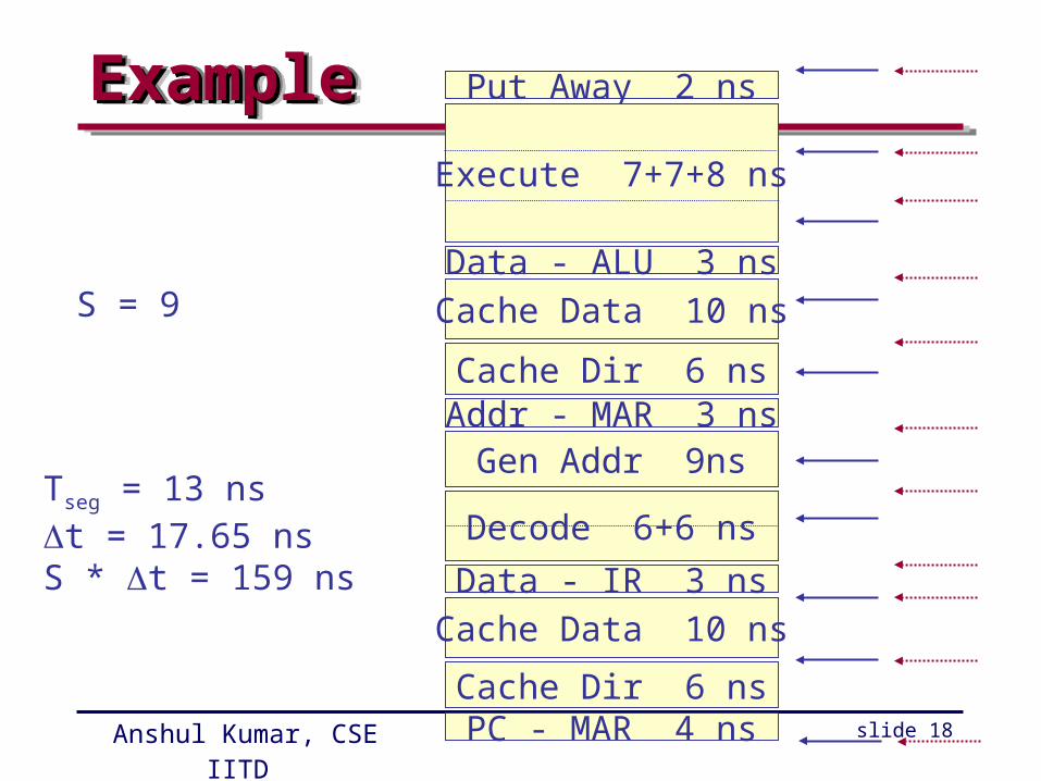
ExampleExampleExampleExample Put Away 2 ns
Data - ALU 3 ns
Addr - MAR 3 ns
Data - IR 3 ns
PC - MAR 4 ns
Cache Dir 6 ns
Cache Dir 6 ns
Cache Data 10 ns
Decode 6+6 ns
Gen Addr 9ns
Cache Data 10 ns
Execute 7+7+8 ns
S = 9
Tseg = 13 nst = 17.65 nsS * t = 159 ns
Anshul Kumar, CSE IITD slide 19
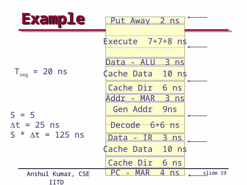
ExampleExampleExampleExample Put Away 2 ns
Data - ALU 3 ns
Addr - MAR 3 ns
Data - IR 3 ns
PC - MAR 4 ns
Cache Dir 6 ns
Cache Dir 6 ns
Cache Data 10 ns
Decode 6+6 ns
Gen Addr 9ns
Cache Data 10 ns
Execute 7+7+8 ns
Tseg = 20 ns
S = 5t = 25 nsS * t = 125 ns
Anshul Kumar, CSE IITD slide 20
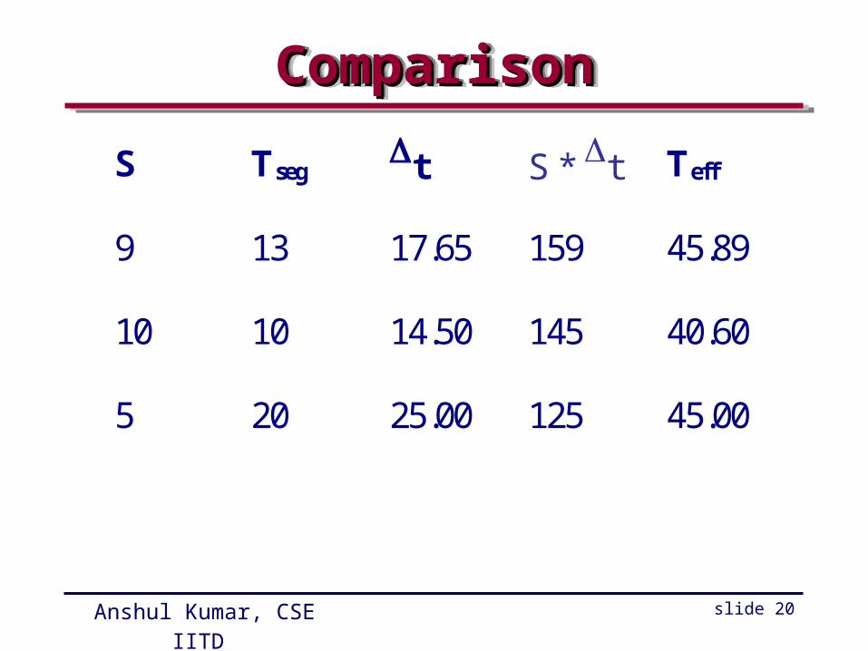
ComparisonComparisonComparisonComparison
S Tseg t S * t Teff
9 13 17.65 159 45.89
10 10 14.50 145 40.60
5 20 25.00 125 45.00
Anshul Kumar, CSE IITD slide 21
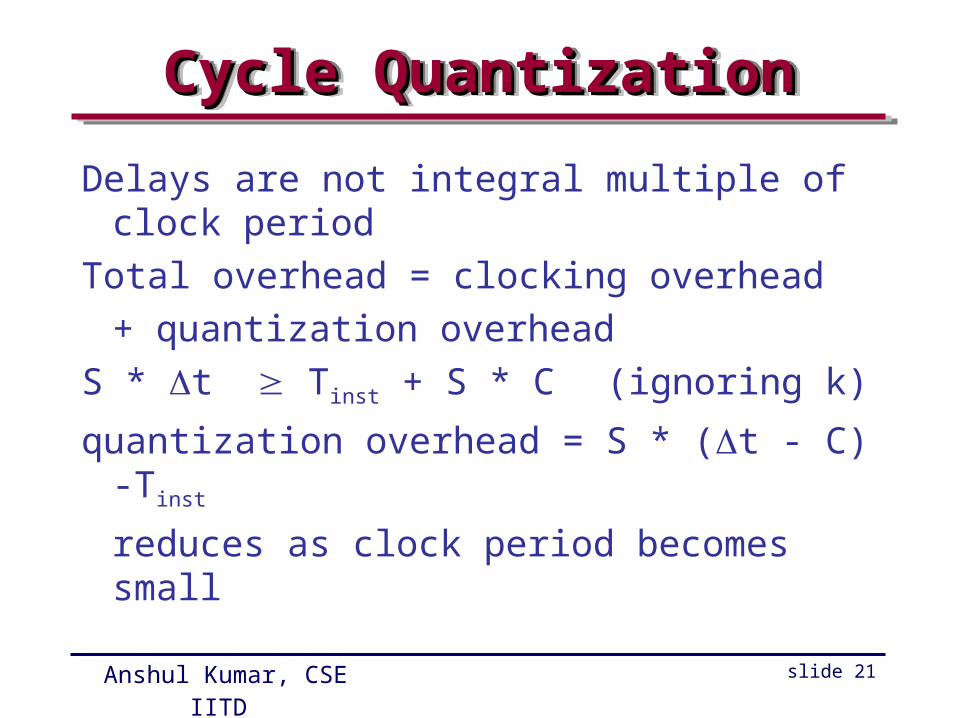
Cycle QuantizationCycle QuantizationCycle QuantizationCycle Quantization
Delays are not integral multiple of clock period
Total overhead = clocking overhead
+ quantization overhead
S * t Tinst + S * C (ignoring k)
quantization overhead = S * (t - C) -Tinst
reduces as clock period becomes small

Anshul Kumar, CSE IITD slide 22
Other Timing ApproachesOther Timing ApproachesOther Timing ApproachesOther Timing Approaches
• Self Timed Circuits– No centralized free running clock– An operation begins as soon as its inputs are
available, that is, all its predecessors have completed
– Higher speed, lower power consumption
• Wave Pipelining– Omit inter-stage registers– Reduced clocking overhead
Anshul Kumar, CSE IITD slide 23
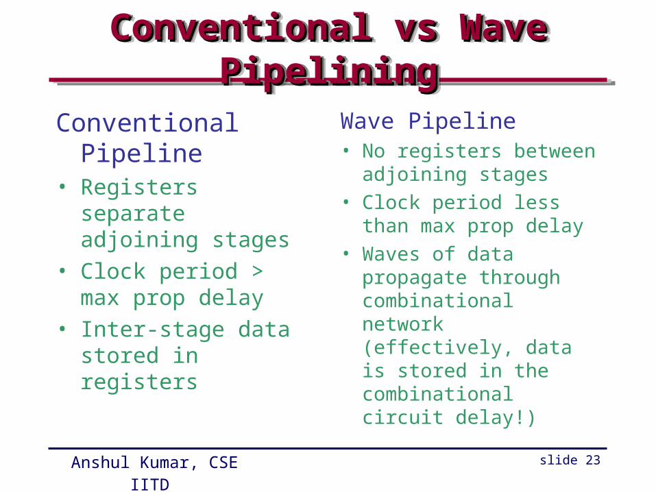
Conventional vs Wave PipeliningConventional vs Wave PipeliningConventional vs Wave PipeliningConventional vs Wave Pipelining
Conventional Pipeline• Registers separate
adjoining stages
• Clock period > max prop delay
• Inter-stage data stored in registers
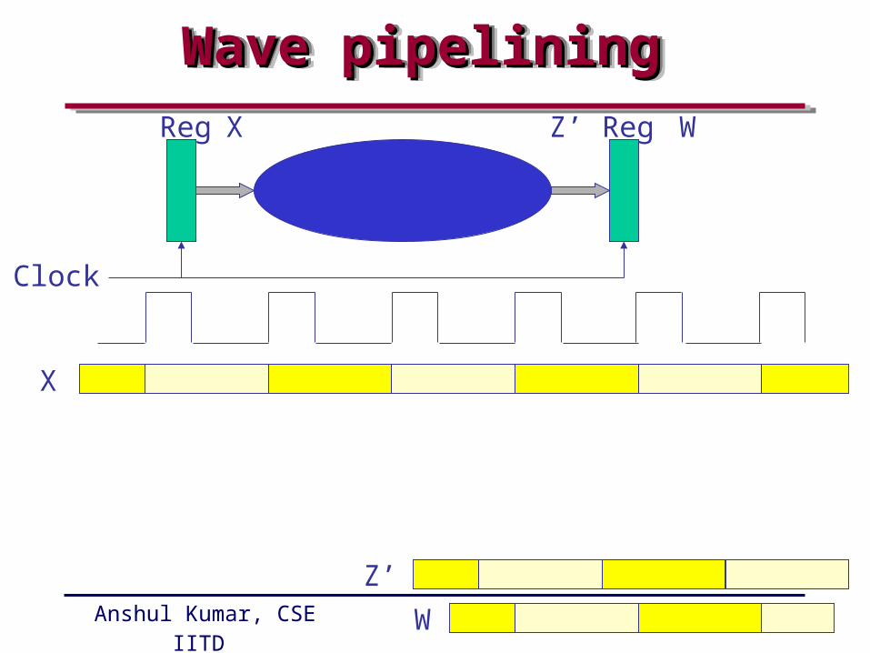
Wave Pipeline• No registers between
adjoining stages
• Clock period less than max prop delay
• Waves of data propagate through combinational network (effectively, data is stored in the combinational circuit delay!)
Anshul Kumar, CSE IITD slide 24
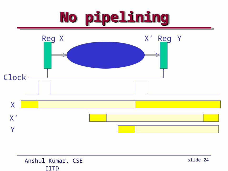
No pipeliningNo pipeliningNo pipeliningNo pipelining
X
Clock
Reg Reg
X
X’ Y
X’
Y
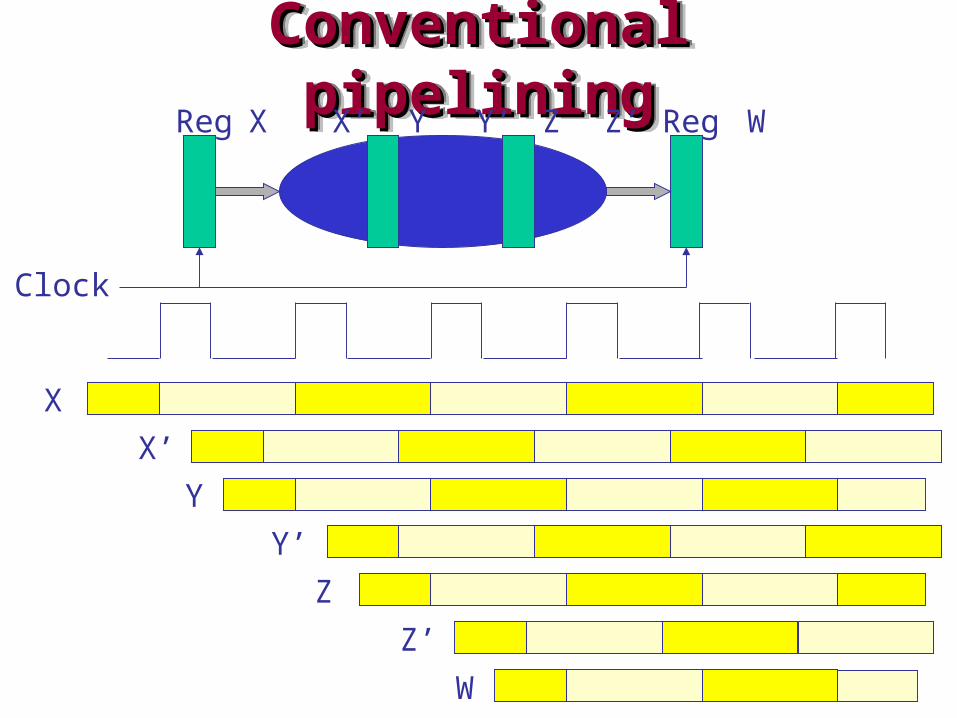
Conventional pipeliningConventional pipeliningConventional pipeliningConventional pipeliningX
Clock
Reg Reg
X
X’ Y Y’ Z Z’ W
X’
Y
Y’
Z
Z’
W
Anshul Kumar, CSE IITD slide 26
Wave pipeliningWave pipeliningWave pipeliningWave pipeliningX
Clock
Reg Reg
X
Z’ W
Z’
W
Anshul Kumar, CSE IITD slide 27
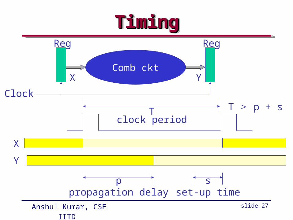
TimingTimingTimingTiming
Comb cktX Y
Clock
Reg Reg
X
Y
ppropagation delay
sset-up time
T p + sTclock period
Anshul Kumar, CSE IITD slide 28
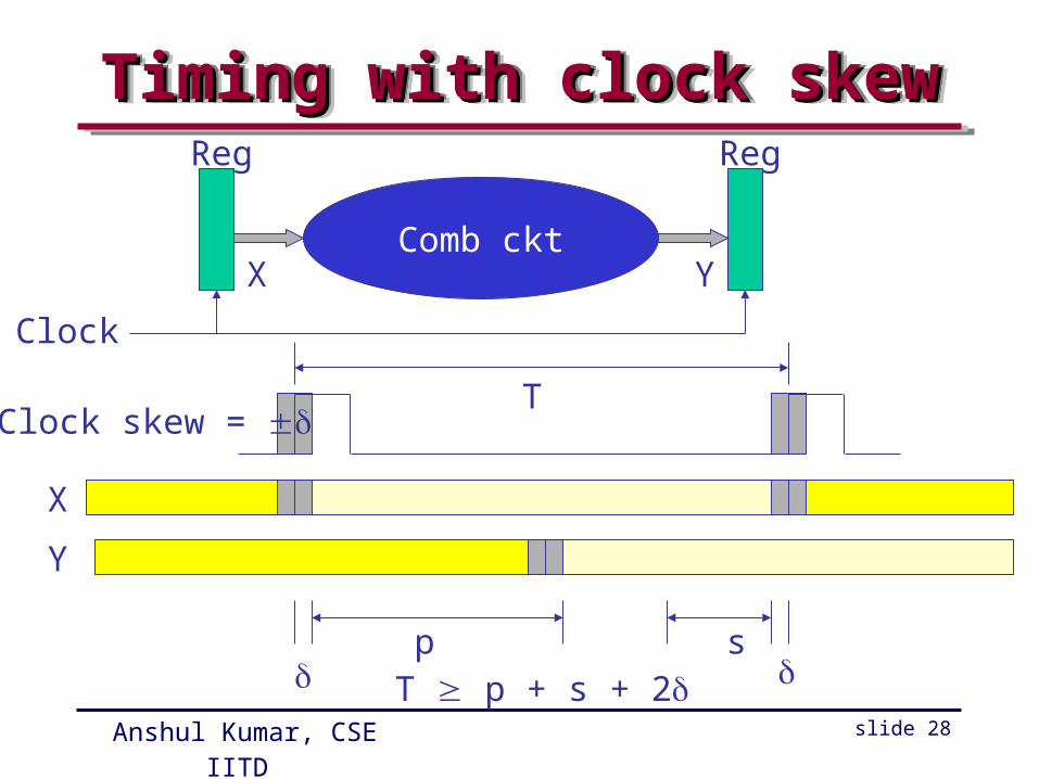
Timing with clock skewTiming with clock skewTiming with clock skewTiming with clock skew
Comb cktX Y
Clock
Reg Reg
X
Y
p s
T
T p + s + 2
Clock skew =
Anshul Kumar, CSE IITD slide 29
Variation in propagation delayVariation in propagation delayVariation in propagation delayVariation in propagation delay
• Different delays in different paths
• Delay variation due to process / temperature/ power variations
• Data-dependent delay variations
Anshul Kumar, CSE IITD slide 30
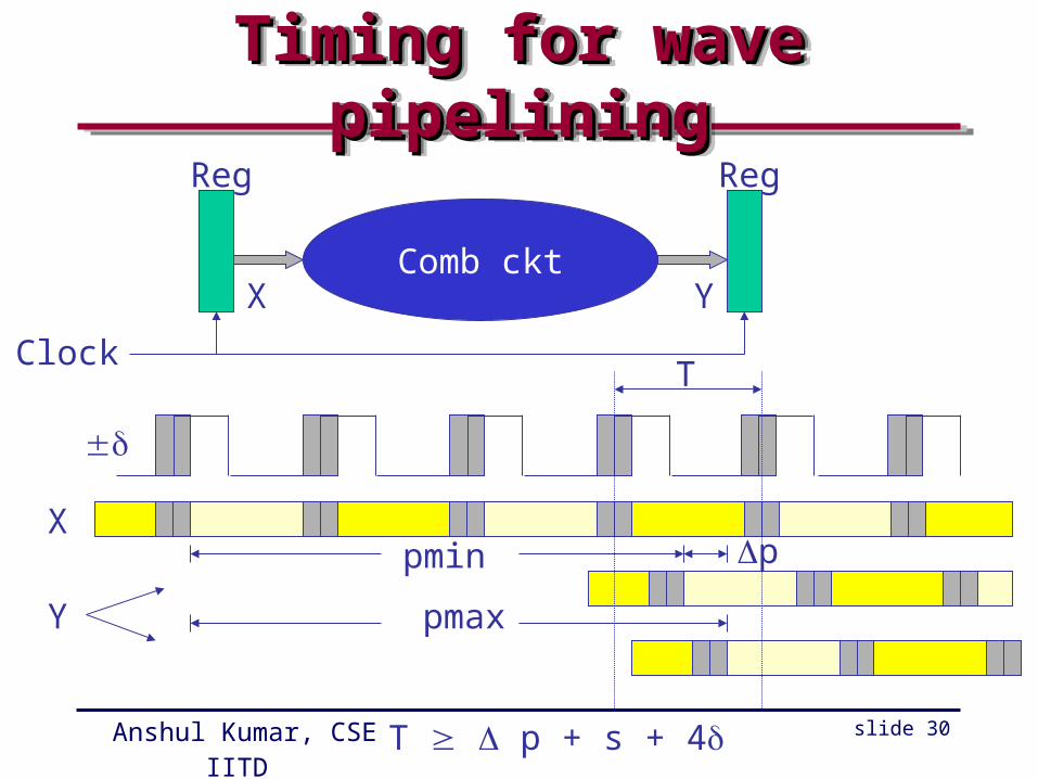
Timing for wave pipeliningTiming for wave pipeliningTiming for wave pipeliningTiming for wave pipelining
Comb cktX Y
Clock
Reg Reg
X
Y
T p + s + 4
pmin
pmax
p
T
Anshul Kumar, CSE IITD slide 31
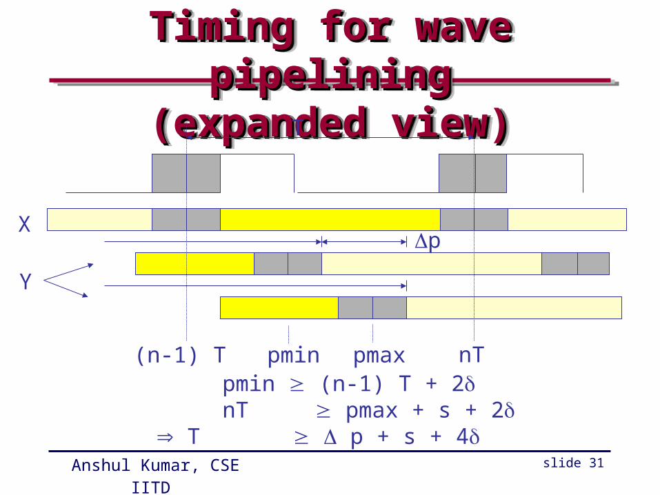
Timing for wave pipeliningTiming for wave pipelining(expanded view)(expanded view)
Timing for wave pipeliningTiming for wave pipelining(expanded view)(expanded view)
pmin (n-1) T + 2 nT pmax + s + 2 T p + s + 4
p
T
X
Y
(n-1) T nTpmin pmax
Anshul Kumar, CSE IITD slide 32
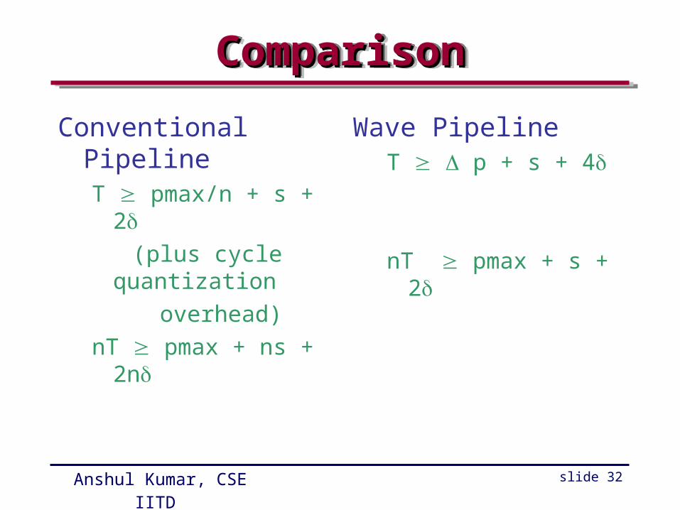
ComparisonComparisonComparisonComparison
Conventional PipelineT pmax/n + s + 2 (plus cycle quantization
overhead)
nT pmax + ns + 2n
Wave PipelineT p + s + 4
nT pmax + s + 2
Anshul Kumar, CSE IITD slide 33
Problems with wave pipeliningProblems with wave pipeliningProblems with wave pipeliningProblems with wave pipelining
• Need to balance delays
• Narrow range of clock frequencies
• Control difficult
• Not very suitable for non-linear pipelines
Anshul Kumar, CSE IITD slide 34
Additional ReadingAdditional ReadingAdditional ReadingAdditional Reading
Wayne P. Burleson, Maciej Ciesielski, Fabian Klass, and Wentai Liu, “Wave-Pipelining: A Tutorial and Research Survey”, IEEE Trans. on VLSI Systems, vol. 6, no. 3, September 1998, pp. 464 – 474.