Econ 100A: Intermediate MicroeconomicsAnswer Key to Problem Set 1

Fall, 2011

Note: This answer key does not contain graphs. For all graphs, refer to thesupplement to this answer key that has been provided alonside.

1. Supply and Demand

Demand Curve: QD = 20− 2PSupply Curve: QS = 2P

a) The inverse demand curve can be obtained by expressing the demandcurve in terms of P. Therefore, we get:Inverse Demad Curve: P = 10 - 1

2QD

The marginal willingness to pay for any unit is just the price of that unit onthe demand curve. Therefore, we can plug Q=5 in the inverse demad curve toget:Marginal willingness to pay = 10 - 2.5 = 7.5

b) To get the equilibrium price, set the quantity demanded equal to thequantity supplied:At equlibrium: 20-2P = 2P⇒ 20 = 4∴ P ∗ = 5Plug the equlibrium value of P into either the demand or the supply function

to get the equlibrium quantity. Plugging P ∗ = 5 into the supply function yields:Q∗ = 2× 5Q∗ = 10

c) Since the demad curve is linear, the price elasticity of demand is given by-mP

Q , where m is the slope of the demand curve.

∴ ε = 2PQAt equlibrium, this takes the value: ε = 2×5

10 = 1Therefore, demand is neither elastic, nor inelastic at this point.

d) Alternative Supply Curve: QS = 5Notice that the quantity supplied is fixed at 5 units. This implies that the

market clearing price is the price which sets the quantity demaded to also be 5.Therefore, we can plug QD = 5 into the inverse demand curve from (a) to get:

1

P = 10 - 12×5

∴ P ∗ = 7.5

e)e.1. Alternative Demand Curve: QD = 30− 2PAt equlibrium with the original supply curve: 30-2P = 2P⇒ P ∗ = 7.5At the original equlibrium in part (a), the market clearing price was 5. With

the alternative specification, the demand curve is shifted out/up, implying thatthe consumers are demanding more at each price. For instance, a vertical inter-cept of 20 in the original demand curve corresponds to the quantity demandedbeing zero at a price of 20. Under the new specification, however, the priceneeds to go up to 30 for the demand to fall to 0. A potential reason for such ashift could be an increase in income.Since the consumers are now demanding more at each price; for a given

supply curve, the market will clear at a higher price. Hence, the shift from 5 to7.5.

e.2. At equlibrium with the alternative supply curve: 30-2P = 5⇒ P ∗ = 12.5Here, too, the equlibrium price is higher than the one we got in part (d).

The reason for this is identical to what was explained above in e.1.Also, notice that the equlibrium price in this case is higher than what we

got in e.1 with the original supply specification. This is because the alternativesupply curve from (d) is perfectly inelastic - the quantity supplied is fixed at 5,and the suppliers are unable to increase it in response to an increase in demand.As a result, the price must climb even higher to accomodate the increase indemand. With the original supply curve, the equlibrium quantity also goes up(to 15), leading to a smaller price increase.

2. Preferences Problem

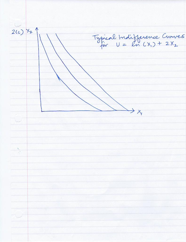
U(x1, x2) = ln(x1) + 2x2

a) Differentiate the utility function with respect to x1 and x2 to get therespective marginal utilities:MU1 = ∂U

∂x1= 1

x1

MU2 = ∂U∂x2

= 2For a person to prefer more to less, his marginal utility must be positive,

i.e., consuming more should add to his total utility.We know that, MU1 =

1x1> 0, for positive values of x1.

Also, MU2 = 2 > 0Therefore, this person prefers more to less.

We can take the second derivative of the utility function to ascertain if themarginal utility is diminishing:

2

∂2U∂x21

= − 1x21< 0

∂2U∂x22

= 0

This utility function exhibits diminishing marginal utility with respect togood 1, and constant marginal utility with respect to good 2.

b) MRS1,2 =MU1MU2

=1x1

2 = 12x1

∂MRS1,2∂x1

= − 12x21

< 0

Therefore, the marginal rate of substitution of good 1 for good 2 is dimin-ishing as the consumption of good 1 is increasing.

c) Note that x1 appears in the utility function as its natural log. We knowthat the log of 0 if not defined - this implies that the consumer always has toconsume a positive amount of x1. Therefore, the indifference curves cannotintercept the x2 axis.We have no such restriction on the consumption of x2. Therefore, we can

have an x1 intercept.

For a plot of the typical indifference curve, refer to the supplementary doc-ument containing graphs.

3. Constrained Optimization Problems:

(Note: There are two alternative ways of doing these problems. This keydemonstrates both methods for part (a), and only 1 for all the problems there-after. You can choose to do either on the exam.)

Budget Constraint: 2F + 4C ≤ 100

a) U(F,C) = F14C

34

Method 1:Set up the Lagrange for optimization:

£ = Max.F,C,λ

F14C

34 + λ(100− 2F − 4C)

First Order Conditions:

F: 14F

− 34C

34 − 2λ = 0 (1)

C: 34F

14C−

14 − 4λ = 0 (2)

λ : 100− 2F − 4C = 0 (3)

Express equation 3 in terms of F:

F = 50− 2C (4)

3

Substitute the value for F in equations 1 and 2, and express in terms of λto get:

18 (50− 2C)

− 34C

34 = λ (1a)

316 (50− 2C)

14C−

14 = λ (2a)

⇒ 18 (

50−2CC )−

34 = 3

16 (50−2CC )

14 (5)

⇒ 50−2CC = 2

3⇒ 150− 6C = 2CC = 150

8 = 754

F = 50− 2× 1508 = 50

4 = 252

Method 2:

At the optimum, the consumer will set the MRS equal to the price ratio:

MRSf,c =14F

− 34C

34

34F

14C− 1

4= 1

3 .CF

PfPc= 1

2

At the optimum: 13 .CF =

12

⇒ CF =

32

∴ C = 32F

Substitute into equation 3:

100− 2F − 4× 32F = 0

100− 8F = 0

⇒ F = 252

C = 32 ×

252 = 75

4

b) U(F,C) = .25 ln(F ) + .75 ln(C)Set up the Lagrange for optimization:

4

£ = Max.F,C,λ

.25 ln(F ) + .75 ln(C) + λ(100− 2F − 4C)First Order Conditions:

F: .25F − 2λ = 0 (1)

C : .75C − 4λ = 0 (2)

λ : 100− 2F − 4C = 0 (3)

Express equation 3 in terms of F:

F = 50− 2C (4)

Substitute the value for F in equation 1, and express in terms of λ to get:.25

2(50−2C) = λ (1a).754C = λ (2a)

⇒ .25100−4C =

.754C

⇒ 4C100−4C = 3

⇒ 4C = 300− 12CC = 150

8 = 754

F = 504 = 25

2

c) U(F,C) = ln(F ) + 4CSet up the Lagrange for optimization:

£ = Max.F,C,λ

ln(F ) + 4C + λ(100− 2F − 4C)First Order Conditions:

F: 1F − 2λ = 0 (1)

C : 4− 4λ = 0 (2)λ : 100− 2F − 4C = 0 (3)

Express equation 3 in terms of F:

F = 50− 2C (4)

Equation 2 ⇒ λ = 1 (5)

Substitute (5) into (1) to get:F = 1

2

5

Substitute the value of F into equation 3 to get:

100− 1− 4C = 0

⇒ C = 994

d) U(F,C) = F + 3CNotice that the two goods are perfect complements, and we will have a corner

solution unless the MRS equals the slope of the price line.

MRSc,f =MUcMUF

= 3PcPF= 2

⇒MRSc,f >PcPF

Therefore, this consumer will only consume clothing at the optimum, andwill choose the quantity that exhausts his budget.

∴ 4C = 100⇒ C = 25F = 0

4. DemandU(F,C) = ln(F ) + ln(C)

Income: I

Price of food: pf

Price of clothing: pc

a) At the optimum, the consumer sets MRS equal to the price ratio, i.e.:

CF =

pf

pc

⇒ pf .F = pc.C (1)

The consumer’s budget constraint is given by:

I − pf .F − pc.C = 0

Substituting (1) into the budget constraint:

6

I − 2pf .F = 0⇒ F = I

2pfDemand Curve for Food

Similarly, calculate demand curve for Clothing:

C = I2pc

b) We know that the demand curve for food is given by:

F = I2pf

∈F,I= ∆F∆I .

IF =

12pf

. IF =1

2pfF

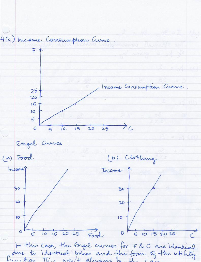
c) We already derived the demand functions for F and C in part a:

F = I2pf

C = I2pc

We can substitute the values for income and prices into this demand functionto derive the optimal basket at each income level:1) I = 10

F = 102×1 = 5

C = 102×1 = 5

2) I = 20F = 20

2×1 = 10

C = 202×1 = 10

3) I = 30F = 30

2×1 = 15

C = 302×1 = 15

For the income consumption curve and the engel curves based on this data,please refer to the supplementary document containing graphs.

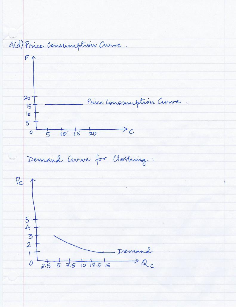
d) I = 30; pf = 1

Note that the demand for food is a function of income and the price of foodalone, both of which are constant. Therefore, as the price of clothing changes,the quantity demanded of food will stay constant at 15.The optimal consumption value of clothing for different values of pc is given

by:

7

1) Pc = 1

C = 302×1 = 15

2) Pc = 2

C = 302×2 = 7.5

3) Pc = 3

C = 302×3 = 5

Therefore, the optimal consumption basket for different values of pc is givenby:

pc = 1: {15,15}pc = 2: {15,7.5}pc = 3: {15,5}

For the price consumption curve and the demand curves based on this data,please refer to the supplementary document containing graphs.

8