Answer to end of chapter solution

Part 1 – Getting Started

Instructor’s Manual to accompanyPublic Finance, Eighth Edition, by Harvey S. Rosen and Ted Gayer

Suggested Answers to End-of-Chapter Discussion Questions

Some of the questions have no single “correct” answer – reasonable people can go off in different directions. In such cases, the answers provided here sketch only a few possibilities.

Chapter 1 - Introduction

1. a. Putin’s statement is consistent with an organic conception of government. Individuals and their goals are less important than the state.

b. Locke makes a clear statement of the mechanistic view of the state in which individual liberty is of paramount importance.

2. Libertarians believe in a very limited government and are skeptical about the ability of government to improve social welfare. Social democrats believe that substantial government intervention is required for the good of individuals. Someone with an organic conception of the state believes that the goals of society are set by the state and individuals are valued only by their contribution to the realization of social goals.

a. A law prohibiting gambling would probably be opposed by a libertarian and advocated by a social democrat. Someone with an organic conception of the state would first decide whether gambling would help to achieve the state’s goals before taking a position on this issue. If the view is that gambling keeps individuals from being productive, then someone with an organic view would probably be in favor of prohibiting it, but if gambling is considered a good way to raise more revenue for the state, then they might oppose the prohibition.

b. Libertarians oppose the law mandating seat belt use, arguing that individuals can best decide whether or not to use seat belts without government coercion. Social democrats take the position that the mandate saves lives and ultimately benefits individuals. The organic view would probably lead to favoring the mandate on the grounds that reduced health care costs caused by fewer accidents benefit society.

c. Libertarians oppose the law mandating child safety seats, arguing that individuals can best decide whether or not to use child safety seats without government coercion. Social democrats take the position that the mandate saves lives and ultimately benefits individuals. The organic view would probably lead to favoring the mandate on the grounds that reduced health care costs caused by fewer accidents benefit society.

1


d. Libertarians would probably oppose a law prohibiting prostitution, while social democrats would likely favor such a law. The organic view depends on the type of society policymakers are attempting to achieve. The law would probably be favored on moral grounds.

e. Libertarians would probably oppose a law prohibiting polygamy, while social democrats would likely favor such a law. The organic view depends on the type of society policymakers are attempting to achieve. The law would probably be favored on moral grounds.

f. Libertarians would likely oppose the law, believing that individual business owners should make the decision about which language is used for their signs. Social democrats would also probably oppose the law in order to foster a more inclusive society. Those with an organic view would probably favor the law if they hold the view that every member of the society should speak the native language.

3. The mechanistic view of government says that the government is a contrivance created by individuals to better achieve their individual goals. Within the mechanistic tradition, people could disagree on the obesity tax. Libertarians would say that people can decide what is best for themselves - whether to consume high calorie food - and do not need prodding from the government. In contrast, social democrats might argue that people are too short sighted to know what is good for them, so that government-provided inducements are appropriate.

4. a. If the size of government is measured by direct expenditures, the mandate does not directly increase it. Costs of compliance, however, may be high and would appear as an increase in a “regulatory budget.”

b. This law would not increase government expenditures, but the high costs of compliance would increase the regulatory budget.

c. It’s hard to say whether this represents an increase or decrease in the size of government. One possibility is that GDP stayed the same, and government purchases of goods and services fell. Another is that government purchases of goods and services grew, but at a slower rate than the GDP. One must also consider coincident federal credit and regulatory activities and state and local budgets.

d. The federal budget would decrease if grants-in-aid were reduced. However, if state and local governments offset this by increasing taxes, the size of the government sector as a whole would not go down as much as one would have guessed.

2


5. The inflation erodes the real value of the debt by 0.016 x £420 billion or £6.72 billion. The fact that inflation reduces the real debt obligation means that this figure should be included as revenue to the government.

6. The federal government grew by $910 billion. However, because the price level went up by 24 percent, in terms of 2005 dollars this amounted to a real increase of $540 billion (=$2.47 trillion - 1.24*$1.56 trillion=$2.47 trillion-$1.93 trillion). As a proportion of GDP, federal spending in 1996 was 19.9 percent ($1.56 trillion/$7.82 trillion) and in 2005 it was 19.8 percent ($2.47 trillion/$12.48 trillion). Hence, the size of government grew in absolute terms and fell slightly in relative terms. To get a more complete answer, one would want data on the population (to compute real spending per capita). Also, it would be useful to add in expenditures by state and local governments, to see if the total size of government fell. Also, although it would be harder to measure, one would want to try to gain some sense of how the regulatory burden on the economy grew during this time period.

7. Relative to GDP, defense spending grew from 4.9 percent of GDP in 1981 to 5.8 percent of GDP in 1985 and then grew from 2.9 percent of GDP in 2001 to 3.8 percent of GDP in 2005. The increase from 2001 to 2005 was proportionally larger.

3


Chapter 2 – Tools of Positive Analysis

1. A change in the marginal tax rate changes the individual’s net wage. This generates both an income effect and a substitution effect. As long as leisure is a normal good, these effects work in opposite directions. Hence, one cannot tell a priori whether labor supply increases or decreases. If there were no political or legal impediments, an experimental study could be conducted in which a control group confronts the status quo, and an experimental group faces the new tax regime. Other things that affect work effort would impact both the control group and the experimental group, so any difference in work effort between the two groups could be attributed to the change in marginal tax rates.

2. This is a valid criticism of the exercise study and the remedy would be to set up a study in which individuals are randomly assigned to groups. In an experimental study, the group engaged in running would not be correlated with good health or a strong heart, so if they enjoyed longer life expectancy, it could be attributed to running instead of other factors.

3. The workers who spend time on a computer probably have other skills and abilities that contribute to higher wages, so training children to use computers would not necessarily cause their earnings potential to improve. This study illustrates the difficulty of determining cause and effect based on correlations. The data do not reveal whether using a computer causes higher earnings, or whether other factors cause workers to use computers and to earn higher wages.

4. The text points out the pitfalls of social experiments: the problem of obtaining a random sample and the problems of extending results beyond the scope of the experiment. Participants in the study had found it to their advantage to be a part of the experiment, which may have resulted in a self-selected population unrepresentative of the wider group of health care consumers. In addition, the RAND Health Insurance Experiment was of limited duration, after which the participants would move to some other health plan. This design could induce certain behavior in the short-run that would not necessarily be present if the health insurance coverage were permanent rather than transitory. Further, physicians’ “standard practices” are largely determined by the circumstances of the population as a whole, not the relatively small experimental group.

5. Random assignment to different class size allows researchers to determine if smaller class size improved test scores, but if some of the students switched classes, the results could be biased. For example, students might be randomly assigned to large classes, but they might have very concerned parents who make an effort to move their children into a smaller class within the same school or at a different school. In such a case, the students’ higher test scores might reflect that they have very involved parents rather than that they were in a smaller class. If, on the other hand, students changed classes or changed schools for other reasons, not related to how they might perform on tests, the results would not be biased.

4


6. Since only five states reduced income taxes, we could examine what happened in a control group of states (those with an income tax but with no change in the tax rates) and compare savings rates between the two. This is important because other factors affect savings rates, but if other factors affected both the control group and the treatment group, then we can conclude that the treatment (lower taxes) caused the change in savings. If, for example, the saving rate for the five states with lower taxes (the treatment group) increased by two percent, while the savings rate for the other states (the control group) increased by one percent, then we could conclude that lower taxes caused the saving rate to increase by one percent—the difference between the two percent increase in the treatment group and the one percent increase in the control group.

7. There is a weak, positive relationship between deficits and interest rates, implying that larger deficits lead to lower interest rates. Inferences based on these data along would be problematic because there are only a few data points and because it would be more informative to look at deficits relative to some benchmark, such as GDP, and to express both interest rates and deficits in real terms, rather than nominal terms. It would also be useful to control for other factors that can affect interest rates, such as monetary policy and the level of economic activity.

5


Chapter 3 – Tools of Normative Analysis

1. a. In this particular insurance market, one would not expect asymmetric information to be much of a problem – the probability of a flood is common knowledge. Moral hazard could be an issue – people are more likely to build near a beach if they have flood insurance. Still, one would expect the market for flood insurance to operate fairly efficiently.

b. There is substantial asymmetric information in the markets for medical insurance for consumers and also malpractice insurance for physicians. For efficient consumption, the price must be equal to the marginal cost, and the effect of insurance may be to reduce the perceived price of medical care consumption. That would lead to consumption above the efficient level. Because of the roles of regulation, insurance, taxes, and the shifting of costs from the uninsured to the insured, there is little reason to expect the market to be efficient.

c. In the stock market, there is good information and thousands of buyers and sellers. We expect, in general, efficient outcomes.

d. From a national standpoint, there is a good deal of competition and information with regards to personal computers. The outcome will likely be efficient for computer hardware. However, some firms might exercise some market power, especially in the software market; in these markets “network externalities” may be present where the value of a programming language or piece of software is dependent on the number of others who also use that software.

e. The private market allocation is likely inefficient without government intervention. Student loan markets may suffer from asymmetric information – the student knows better than the lender whether he will repay the loan or default on it, a form of adverse selection. Government intervention does not “solve” the adverse selection problem in this case (because participation in the student loan program is not compulsory), but it may create a market that would not exist without intervention.

f. There are several reasons why automobile insurance provision is likely to be inefficient without government intervention. As with other insurance markets, the automobile insurance market suffers from asymmetric information. Drivers who know they are particularly accident prone will be particularly likely to want car insurance (or policies with greater coverage), while drivers who are less accident prone (or able to self-insure) might choose to go without insurance. By mandating that people purchase auto insurance if they choose to drive, the adverse selection problem is mitigated to some extent (but, again, more accident prone drivers could still by more generous plans). Another market imperfection, related to “underinsurance” has to do with the financial externalities from an automobile accident. An uninsured motorist who is at fault may not have sufficient income to cover the costs of the other driver’s bills, and instead default on the obligation by

6


g. declaring bankruptcy. The bankruptcy “floor” on costs creates various moral hazard problems.

2. Point a represents an equal allocation of water, but it is not efficient because there is no tangency. Point b is one of many Pareto efficient allocations, representing a case where Catherine benefits enormously by trade, and Henry’s utility is unchanged from the initial endowment.

AD: 1) The dashed line is positioned at the halfway point on the horizontal axis.2) Point b is a tangency

3. If insurers in California could no longer use location to determine automobile insurance rates, some of the higher costs incurred by urban residents would be shifted to rural and suburban residents. This change would reduce efficiency, but the purpose of the policy is to improve equity, based on an argument that it is unfair that urban residents should have to pay more for insurance because they are more likely to be involved in accidents. Social welfare increases if the additional utility enjoyed by urban residents offsets the loss in utility to rural and suburban residents.

7


4. a. Social indifference curves are straight lines with slope of –1. As far as society is concerned, the “util” to Augustus is equivalent to the “util” to Livia.

8


b. Social indifference curves are straight lines with slope of –2. This reflects the fact that society values a “util” to Augustus twice as much as a “util” to Livia.

9


5. Musgrave (1959) developed the concept of merit goods to describe commodities that ought to be provided even if the members of society do not demand them. “Sin taxes” work the opposite way and apply to commodities that members of society might demand, but ought not to have.

6. a. There is no obvious reason why there is a market failure with burglar alarm calls; the Los Angeles police could set a response fee equal to the marginal cost.

b. Welfare economics provides little basis for such a subsidy of wool and mohair production.

c. There is no economic reason why cherry pies should be regulated, especially since there are no such regulations for apple, blueberry, or peach frozen pies.

d. It is hard to imagine a basis in welfare economics for this regulation for hairdressers.

e. This is not an efficient policy. If the problem is that too much water is being consumed, then the answer is to increase the price of water. On that basis, people can decide whether or not they want to buy toilets that require less water. Water, like most other resources, is a private good.

f. There is no economic reason why the federal government should subsidize the production of electricity, whether the electricity comes from coal, nuclear power, or chicken manure. One can assume the question that the R&D process of creating electricity from chicken manure is already developed, so there is not a positive externality argument. Since the production of electricity is a private good, with no obvious violations of the fundamental welfare theorem, there is no justification.

7. In this case, the “Edgeworth box” is actually a line because there is only one good on the island. The set of possible allocations is a straight line, 100 units long. Every allocation is Pareto efficient, because the only way to make one person better off is to make another person worse off. There is no theory in the text to help us decide whether an allocation is fair. Although splitting the peanuts even between the people may be fair, it may not be fair if the calorie “needs” of the people are different. With a social welfare function, we can make assessments on whether redistribution for society as a whole is a good thing.

8. Social welfare is maximized when Mark’s marginal utility of income is equal to Judy’s marginal utility of income. Taking the derivative of Mark’s utility function to find his marginal utility function yields MUM = 50/(IM

1/2) and taking the derivative of Judy’s utility function yields MUJ = 100/(IJ

1/2). If we set MUM equal to MUJ, the condition for maximization becomes IJ = 4IM and, since the fixed amount of income is $300, this means that Mark should have $60 and Judy should have $240 if the goal is to maximize social welfare = UM + UJ.

10


9. Although Victoria’s marginal rate of substitution is equal to Albert’s, these are not equal to the marginal rate of transformation and the allocation is, therefore, Pareto inefficient. Both people would give up 2 cups of tea for 1 crumpet but, according to the production function, could actually get 6 crumpets by giving up 2 cups of tea. By giving up tea and getting crumpets through the production function, both utilities are raised.

10. a. False. As shown in the text, equality of the marginal rates of substitution is a necessary, but not sufficient, condition. The MRS for each individual must also equal the MRT.

b. Uncertain. As long as the allocation is an interior solution in the Edgeworth box, the marginal rates of substitution must be equal across individuals. This need not be true, however, at the corners where one consumer has all the goods in the economy.

c. False. A policy that leads to a Pareto improvement results in greater efficiency, but social welfare depends on equity as well as efficiency. A policy that improves efficiency but creates a loss in equity might reduce social welfare.

d. Uncertain. The tax reduces efficiency, but if education creates positive externalities, then increased funding for education improves efficiency. This is a Pareto-improving policy if the increased efficiency in the education market more than offsets the reduced efficiency in the market for cigarettes.

11


Chapter 4 – Public Goods

1. a. Wilderness area is an impure public good – at some point, consumption becomes nonrival; it is, however, nonexcludable.

b. Satellite television is nonrival in consumption (although it is excludable).

c. Medical school education is a private good.

d. Television signals are nonrival in consumption.

e. An Internet site is nonrival in consumption (although it is excludable).

2. a. False. Efficient provision of a public good occurs at the level where total willingness to pay for an additional unit equals the marginal cost of producing the additional unit.

b. False. Due to the free rider problem, it is unlikely that a private business firm could profitably sell a product that is non-excludable. However, recent research reveals that the free rider problem is an empirical question and that we should not take the answer for granted. Public goods may be privately supported through volunteerism, such as when people who attend a fireworks display voluntarily contribute enough to pay for the show.

c. Uncertain. This statement is true if the road is not congested, but when there is heavy traffic, adding another vehicle can interfere with the drivers already

using the road.

d. False. There will be more users in larger communities, but all users have access to the quantity that has been provided since the good is non-rival, so there

is no reasons larger communities would necessarily have to provide a larger quantity of the non-rival good.

3. We assume that Cheetah’s utility does not enter the social welfare function; hence, her allocation of labor supply across activities does not matter.

a. The public good is patrol; the private good is fruit.

b. Recall that efficiency requires MRSTARZAN + MRSJANE = MRT. MRSTARZAN = MRSJANE = 2. But MRT = 3. Therefore, MRSTARZAN + MRSJANE MRT. To achieve an efficient allocation, Cheetah should patrol more.

4. Research on alternative medicine is a public good if the research leads to treatments or cures that are non-excludable, meaning that others besides those who discovered the treatment may profit from the treatments. This would happen if discoveries cannot be patented. Whether or not it is sensible for government to pay for such research depends on the potential benefits of the research, which could be substantial if alternative

12


medicine provides effective treatments, and whether or not the treatments can be patented.

5. Aircrafts are both rival and excludable goods, so public sector production of aircrafts is not justified on the basis of public goods. If policymakers assume that the benefits of the mega-jetliner are public, then they would find the efficient level of production by vertically summing demand curves rather than horizontally summing demand curves. This causes the benefits to be significantly overstated and could be used to justify such high costs.

13


6. This debate is similar to the debate about private versus public education. Public sector production is often associated with higher costs (for both schools and prisons), but there may be other reasons society would prefer public to private provision. These reasons typically relate to equity considerations. For schools, the main argument is to make sure everyone child has the opportunity for a good education. For prisons, there may be a fundamental conflict between fair and humane treatment of prisoners and keeping costs low. For example, equity might require that prisoners be fed nutritious meals, but giving them bread and water for every meal might be less expensive. This question asks students to give personal opinions about privatizing prisons, so there is no single “right” answer.

7. The experimental results on free-riding suggest that members of the community might voluntarily contribute about half of the required amount. The reason these citizens wanted to use private fundraising was because the state government redistributed tax dollars from wealthy districts to poor districts (the so-called Robin Hood plan), so using private donations was a way to avoid losing tax dollars to other districts.

8. There is no compelling reason for museums to be run by the government from the theory of public goods; thus, it is appropriate to think about privatization. Admissions to museums are clearly excludable. And viewing the artwork is also rival, because there is congestion when too many people are consuming the good. Thus, museums may be thought of as a private good rather than public good. In the United States, many great museums are run privately (not for profit), and they seem to do quite well. In terms of private versus public production, the text points out that this decision should be based on relative wage and material costs in the public and private sector, administrative costs, diversity of tastes, and distributional issues. There is no compelling reason to think the private sector would have higher costs than the public sector. In regards to diversity of tastes, a profit-maximizing private sector museum would likely be more responsive to consumer tastes than the public sector – e.g., adopting new technologies that make the museum more enjoyable for the typical customer. In regards to distributional issues, it is likely that the private sector would be less responsive than the public sector. The notion of commodity egalitarianism, however, is a stretch for museums.

9. a. Zach’s marginal benefit schedule shows that the marginal benefit of a lighthouse starts at $90 and declines, and Jacob’s marginal benefit starts at $40 and declines. Neither person values the first lighthouse at its marginal cost of $100, so neither person would be willing to pay for a lighthouse acting alone.

b. Zach’s marginal benefit is MBZACH=90-Q, and Jacob’s is MBJACOB=40-Q. The marginal benefit for society as a whole is the sum of the two marginal

benefits, or MB=130-2Q (for Q≤40), and is equal to Zach’s marginal benefit schedule afterwards (for Q>40). The marginal cost is constant at MC=100, so the intersection of aggregate marginal benefit and marginal cost occurs at a quantity less than 40. Setting MB=MC gives 130-2Q=100, or Q=15. Net benefit can be measured as the area between the

14


demand curve and the marginal benefit of the 15th unit. The net benefit is $112.5 for each person, for a total of $225.

15


10. Thelma’s marginal benefit is MBTHELMA=12-Z, and Louise’s is MBLOUISE=8-2Z. The marginal benefit for society as a whole is the sum of the two marginal benefits, or MB=20-3Z (for Z≤4), and is equal to Thelma’s marginal benefit schedule afterwards (for Z>4). The marginal cost is constant at MC=16. Setting MB=MC along the first segment gives 20-3Z=16, or Z=4/3, which is the efficient level of snowplowing. Note that if either Thelma or Louise had to pay for the entire cost herself, no snowplowing would occur since the marginal cost of $16 exceeds either of their individual marginal benefits from the first unit ($12 or $8). Thus, this is clearly a situation when the private market does not work very well. Also note, however, that if the marginal cost were somewhat lower, (e.g., MC≤8), then it is possible that Louise could credibly free ride, and Thelma would provide the efficient allocation. This occurs because if Thelma believes that Louise will free ride, Thelma provides her optimal allocation, which occurs on the second segment of society’s MB curve, which is identical to Thelma’s MB curve (note that Louise gets zero marginal benefit for Z>4). Since Louise is completely satiated with this good at Z=4, her threat to free ride is credit if Thelma provides Z>4.

16


Chapter 5 - Externalities

1. Classical economics explicitly requires that all costs and benefits be taken into account when assessing the desirability of a given set of resources, so Gore’s statement is false. The notion that rescuing the environment should be “the central organizing principle for civilization” provides no practical basis for deciding what to do about automobile emissions (or any other environmental problem), because it provides no framework for evaluating the tradeoffs that inevitably must be made.

2.

a. The number of parties per month that would be provided privately is P.

b. See schedule MSBp.

c. P*. Give a per-unit subsidy of $b per party.

d. The total subsidy=abcd. “Society” comes out ahead by ghc, assuming the subsidy can be raised without any efficiency costs. (Cassanova’s friends gain gchd; Cassanova loses chd but gains abcd, which is a subsidy cost to government.)

3. a. It is very likely that the farmer could negotiate with the neighbors, provided property rights are clearly defined. The Coase Theorem is therefore applicable.

b. It is unlikely that property rights could be enforced in terms of catching tropical fish on the Amazon River. The question states that hundreds of divers illegally catch these fish and sell them on the black market. If the property rights were given to the divers, it is not clear who is actually harmed (perhaps “society as a whole”) by the depletion of exotic fish. Given the large number of people who are harmed (in a small amount), and the large number of people who are engaging in this activity, it is not clear how bribes would flow from “society” to the “divers.”

c. There are too many farmers and too many city-dwellers for a private negotiation.

d. Too many people are involved for private negotiation and impossible to figure out how to transfer bribes.

17

TGRs

$

104.5 billion

Supply of TGRs

Demand for TGRs

$0.75


4. a. The price of imported oil does not reflect the increased political risk byeffectively subsidizing authoritarian regimes like those in Saudi Arabia.

b. The tax would estimate the marginal damage (e.g., the increased instability in the Middle East, etc.) by importing oil from Saudi Arabia.

c. The supply of TGRs is vertical at 104.5 billion if government seeks to reduce consumption of gasoline to 104.5 billion. Consumers must have one TGR in order to buy one gallon of gasoline, plus they must pay the price at the pump. Limiting TGRs effectively limits the demand for gasoline, so the price per gallon will fall, but consumers must have TGRs in order to purchase gasoline. If the market price of one TGR is $0.75, this means that supply and demand intersect at $0.75, as shown in the graph. This kind of program curbs consumption without giving government more revenue because consumers are purchasing the TGRs from each other. However, the total amount of TGRs is limited by government. Those consumers seeking to purchase more gasoline than allowed by the initial allocation of TGRs can purchase additional TGRs from other consumers at the market price of $0.75. By choosing to use a TGR to purchase gasoline, a consumer incurs an opportunity cost equal to $0.75 since they cannot sell the TGR once it has been used.

5. The use of the drug to treat sick cows leads to a positive externality (the benefit enjoyed by air travelers) as well as a negative externality (the costs created by a larger number of rats and feral dogs). Banning the drug might raise or lower efficiency, depending on whether the positive externality is larger or whether the negative externality is larger.

18


There are many ways to design incentive-based regulations. Policymakers could determine the efficient level of drug usage and then either allocate or sell the right to use the drug for sick cows.

6. There are many policy alternatives for addressing problems with traffic congestion. Most of these focus on reducing the number of vehicles on the road during high-traffic times, whether through regulation or through incentive-based programs.

7. a. When the Little Pigs hog farm produces on its own, it sets marginal benefitequal to marginal cost. This occurs at 4 units.

b. The efficient number of hogs sets marginal benefit equal to marginal social cost, which is the sum of MC and MD. At 2 units, MB=MSC=13.

c. The merger internalizes the externality. The combined firm worries about the joint profit maximization problem, not the profit maximization problem at either firm alone. Thus, the LP farm produces 2 units, the socially efficient amount.

d. Before the merger, the LP farm produced 4 units. By cutting back to 2 units, it loses marginal profit of $3. On the other hand, the Tipsy Vineyard’s profits increase by $20. Thus, profits increase by $17 altogether.

8. Private Marginal Benefit = 10 - X

Private Marginal Cost = $5

External Cost = $2

Without government intervention, PMB = PMC; X = 5 units.

Social efficiency implies PMB = Social Marginal Costs = $5 + $2 = $7; X = 3 units.

Gain to society is the area of the triangle whose base is the distance between the efficient and actual output levels, and whose height is the difference between private and social marginal cost. Hence, the efficiency gain is ½ (5 - 3)(7 - 5) = 2.

A Pigouvian tax adds to the private marginal cost the amount of the external cost at the socially optimal level of production. Here a simple tax of $2 per unit will lead to efficient production. This tax would raise ($2) (3 units) = $6 in revenue.

9. In the absence of persuasive evidence on positive externalities for higher education, there is no efficiency reason for the government to provide a free university education. Society may decide that a more equitable distribution of income is achieved by subsidizing higher education, but this is a debate involving value judgments.

19


10. a. The total cost of emissions reduction is minimized only when the marginal costs are equal across all polluters, therefore a cost-effective solution requires

that MC1 = MC2 or that 300e1 = 100e2. Substituting 3e1 for e2 in the formula e1 + e2 = 40 (since the policy goal is to reduce emissions by 40 units) yields the solution. It is cost-effective for Firm 1 to reduce emissions by 10 units and for Firm 2 to reduce emissions by 30 units.

b. In order to achieve cost-effective emission reductions, the emissions fee should be set equal to $3,000. With this emissions fee, Firm 1 reduces 10 units and Firm 2

reduces 30 units, but Firm 1 has to pay $3,000 for each unit of pollution they continue to produce, which gives them a tax burden of $3,000 x 90 (Firm 1 generated 100 units in the absence of government intervention) or $270,000. Firm 2 has a lower tax burden because it is reducing emissions from 80 units to 50 units. Firm 2 pays $3,000 x 50 = $150,000. As the text concludes, the firm that cuts back pollution less isn’t really getting away with anything because it has a larger tax liability than if it were to cut back more.

c. From an efficiency standpoint, the initial allocation of permits does not matter. If the two firms could not trade permits, then Firm 2 would have to

undertake all of the emissions reduction. Initially, Firm 1’s MC is zero, while Firm 2’s MC is $4,000, so there is a strong incentive for Firm 2 to purchase permits from Firm 1. Trading should continue until MC1 = MC2, which is the cost-effective solution. This means that the market price for permits will equal $3,000, the same as the emissions fee. At this price, Firm 2 will purchase 10 permits from Firm 2, allowing Firm 2 to reduce emissions by 30 rather than 40 and requiring Firm 1 to reduce emissions by 10. This solution is the same as the solution achieved with the emissions fee. However, Firm 1 is better off because instead of having to pay taxes, it will receive a payment of $30,000 for its permits. Firm 2 must pay $30,000 for the extra permits, but it also avoids the payment of taxes. The government lost $420,000 in tax revenue. The firms must still pay the cost of emissions reduction, plus Firm 2 must pay for the permits purchased from Firm 1.

11. If marginal costs turn out to be lower than anticipated, cap-and-trade achieves too little pollution reduction and an emissions fee achieves too much pollution reduction. With an inelastic marginal social benefit function, cap-and-trade is not too bad from an efficiency standpoint, while an emissions fee causes pollution reduction to be much greater than the efficient level when marginal cost is lower than anticipated. When marginal social benefits are elastic, the opposite is true.

20


Chapter 6 – Political Economy

1. a. Below, the preferences for Person 1 and Person 2 are drawn. Same procedure is used for the other three people.

b. C wins in every pairwise vote. Thus, there is a stable majority outcome, despite the fact that persons 1, 2, and 3 have double-peaked preferences. This demonstrates that although multi-peaked preferences may lead to voting inconsistencies, this is not necessarily the case.

2. The belief that the tax bill will pass because it contains provisions sought by so many different lawmakers is consistent with the logrolling model. It could be the case that each lawmaker has inserted favored provisions with the understanding that other lawmakers will support the overall package provided it contains the provisions they favor.

3. Without vote-trading, neither bill would pass. If there is vote-trading, then voter B would agree to support issue X provided voter A supports Issue Y, allowing both bills to pass. The change in net benefits is +3 for Issue X and -2 for Issue Y, so logrolling results in a gain of +1.

4. Yes, it is consistent, because the theory says that when unanimity is required, no decisions are likely to be made. A majority system might be more suitable, although it is subject to cycling and other problems.

5. Assuming that the preferences of Kuwaiti women differ from the preferences of Kuwaiti men, stronger voter turnout by women could invalidate the median voter theorem. That is, the results of majority voting would not reflect the preferences of the median voter.

6. When there is a vote over five options, there is the chance that a potential majority vote is split between four relatively preferred options, and the fifth option wins. The winning

21


option may have been voted down if it had been a two-way vote with any of the other options. Further, if preferences are not single-peaked, cycling and inconsistent public decisions may emerge.

22


7. Given the U.S. experience with the Budget Enforcement Act of 1990, we would expect the EU deficit limits to be ineffective. We would expect “accounting tricks” to mask the size of the deficits (such as itemizing various budget items as “unexpected emergencies”), and if that didn’t work, we would expect the deficit rules to be ignored. This is apparently what is happening. When Germany exceeded the deficit target, no moves were taken to levy the required fines.

8. Since rents, by definition, are the returns above a normal return, then when the licenses are put on the market, their price will be the value of the rents. Hence, the owner of the peanut license, whoever he or she is, only makes a normal return. Put another way, the license is an asset that earns a normal rate of return. If the peanut license system were eliminated, efficiency would be enhanced. But the elimination would, in effect, confiscate the value of this asset. It is not clear that this is fair. One could also argue that when someone buys this asset, the purchase is with the understanding that there is some probability that its value will be reduced by elimination of the program; hence, it is not unfair to do so.

9. a. With the demand curve of Q=100-10P and a perfectly elastic supply curve at P=2, then the milk is sold at a price of $2, and a quantity of 80 units is sold.

b. The marginal revenue curve associated with the inverse demand curve P=10-(1/10)Q is MR=10-(1/5)Q, while the marginal cost curve is MC=2. The cartel would ideally produce a quantity where MR=MC, or 10-(1/5)Q=2, or Q=40. The price associated with a cartel quantity of 40 units is P=10-(1/10)*40, or P=6.

c. The rent associated with the cartel is the product of the marginal profit per unit and the number of units produced. The marginal profit per unit of milk is $4 (=$6 price - $2 marginal cost), while 40 units are produced. Thus, the rents equal $160.

d. The most the cartel would be willing to contribute to politicians is the full economic rent of $160. The cartel situation, the quantity of milk produced is too low from society’s point of view. The deadweight loss triangle is computed using the difference between the cartel output and competitive output as the “base” of the triangle, and the difference between the cartel price and competitive price as the “height.” Thus, the triangle is equal to (1/2)*(80-40)*($6-$2)=$40.

e. As Figure 6.5 in the textbook shows, the deadweight loss could now go as high as the sum of the conventional deadweight loss and the rents, or $160 rents + $80 DWL = $240. This is because, as noted in the text, “rent-seeking can use up resources – lobbyists spend their time influencing legislators, consultants testify before regulatory panels, and advertisers conduct public relations campaigns. Such resources, which could have been used to produce new goods and services, are instead consumed in a struggle over the distribution of existing goods and services. Hence, the rents do not represent a mere lump-sum transfer; it is a measure of real resources used up to maintain a position of market power.”

23


24


10. Niskanen’s model of bureaucracy is illustrated in Figure 6.4 of the textbook. In the aftermath of September 11th, the new concerns over food safety would likely shift the V curve upward (that is, the value placed on each level of Q). Assuming that C curve (costs per unit of Q) does not change, then this shift increases the actual number of food inspectors hired. It is also likely that the slope of the V curve changes, with each marginal unit of Q becoming more valuable. Thus, the V curve not only “shifts” upward, but becomes steeper as well. Both of these effects – the shifting of the V curve and the change in the slope – lead to greater values of Q under the bureaucracy model. The change in the slope leads to a greater value of Q*, the efficient level of output. Thus, the optimal number of FDA employees and the actual number of FDA employees are likely to rise.

11. a. The outcome of the first election (M vs. H) is M. The outcome of the second election (H vs. L) is L. The outcome of the third election (L vs. M) is M. Majority rule leads to a stable outcome since M defeats both H and L. Giving one person the ability to set the agenda would not affect the outcome in this case.

b. With the change in Eleanor’s preference ordering, majority rule no longer generates a stable outcome. In a vote between M and H, the outcome is H. In a vote between H and L, the outcome is L. In a vote between L and M, the outcome is M. So, giving one person the ability to set the agenda affects the outcome. For example, Abigail prefers H, so she might pit L against M first in order to eliminate L and avoid having L defeat H.

25

ep

BA

A

Other Goods

Education

Parents can supplement public education with private lessons


Chapter 7 – Education

1. There are numerous rationales given for government provision of education. Even though education is primarily a private good, many argue that educating a child provides external benefits. However, the existence of a positive externality implies that government should subsidize education rather than making it free and mandatory. Other rationales are based on equity, including a belief in commodity egalitarianism.

2. If households are allowed to supplement public education with private lessons, then the budget constraint in Figure 4.5 of the textbook is modified by drawing a line starting at point x (consuming only public education) that runs to the southeast and is parallel to AB. The figure below is then similar to the analysis of in-kind benefits like food stamps.

26

DC

ep

BA

A

Other Goods

Education

Public School is financed by taxes levied on parents


If parents pay for the public schooling (rather than perceiving it as being free), and the schooling was paid for with a lump sum tax, then the budget constraint shifts in by an amount that depends on the household’s share of the tax burden. If the household’s tax burden exactly equals the cost of public school, the budget constraint is no longer the line segment AB but rather the segment CDB, where the segment DB runs along the original budget constraint, except that the minimum amount of schooling consumed is eP.

3. The question distinguishes between a private market for higher education, in which students would have to pay their own tuition, and a system of taxpayer-financed higher education. The examples cited in France and Germany illustrate a third option of little or not support of higher education from either private tuition dollars or public tax dollars. If a government disallows either type of support, then the result will be very little higher education, or low-quality higher education. For most, the debate centers on the choice between private support and public support. Some may conclude that efficiency is served by providing financial support using tax dollars because the free market solution is less than the socially efficient solution when significant positive externalities are present. To make this argument, it is important to provide evidence that there are significant positive externalities. Remember that as long as the earnings of college graduates reflect their higher productivity, the belief that higher education causes workers to become more productive does not imply the existence of an externality. From an equity standpoint, subsidies for college students represent a transfer from taxpayers to college students, so subsidizing higher education may or may not result in a more equitable distribution of income.

27


28

Other Goods

Education$50,000

$50,000

Other Goods

Education$8,000

$50,000

$50,000


4. a. If income is $50,000 per year, the budget constraint is a straight line, as shown below.

b. With $8,000 worth of free public education, the family can consumer up to $8,000 worth of education without reducing the consumption of other goods.

29

Other Goods

Education$8,000

.

.A

B$50,000

$50,000


c. The family maximized utility at point A before the introduction of free public education, and maximizes utility at point B after free public education is introduced, so the optimal consumption of education fell.

30

Other Goods

Education$8,000

.A

B.$50,000

$50,000 $58,000


d. With an $8,000 education voucher, the family can spend some of its income on education to purchase more education if it desires. If the optimal point moves from A to B, as shown in the graph below, then the introduction of vouchers causes the family to purchase more education.

5. a. The results might be biased if there are other differences between the two states. For example, parents might have greater educational attainment in the state whose teacher’s have master’s degrees and the higher test scores could reflect this rather than the difference in teachers’ educational attainment.

b. The experimental study provides stronger evidence that students whose teachers have master’s degrees will score higher on tests because students were randomly assigned to be in the control group or the treatment group.

31


Chapter 8 – Cost Benefit Analysis

1. Yes, one really must ask these questions, although it may seem distasteful. Otherwise, there is no way to determine which safety precautions are sensible.

2. The increased time spent at the inspection must be counted as a cost of the program. One reasonable way to estimate the value of the time would be to use the average wage rate in the state, and multiply this by the incremental waiting time of 105 minutes.

3. The present value of $25/.10 = $250.The present value of the perpetual annual benefit = B + B/(1 + r) + B/(1 + r)2 + … = B (r + 1 - r)/r = B/r.

4. a. The internal rate of return is the discount rate that would make the project’s net present value (NPV) equal zero. To solve for the internal rate of return, ,

set the present value of benefits minus the present value of costs equal to zero. If we assume the benefit of using the bicycle is immediate (and worth $170), there is also the benefit of re-selling the bicycle for $350, but it can’t be re-sold until next year, so must be discounted. Therefore, NPV is 170 + [350/(1+)] – 500 = 0. Solving this expression for yields = 6 percent. If we assume that the benefits of the vacation will not be enjoyed for one year, then NPV is [(170+350)/(1+)] – 500 and setting this expression equal to zero and solving for yields = 4 percent.

b. If the discount rate is 5 percent, purchasing the bicycle is a good idea if is 6 percent, but a bad idea if is 4 percent.

5. a. Bill is willing to pay 25 cents to save 5 minutes, so he values time at 5 cents per minute. The subway saves him 10 minutes per trip, or 50 cents. The value of 10 trips per year is $5. The cost of each trip is 40 cents, or $4 per year. The annual net benefit to Bill is therefore $1. The present value of the benefits = $5/.25 = $20; the present value of the costs is $4/.25 = $16.

b. Total benefits = $20x55,000=$1,100,000.Total costs = $16x55,000 = $880,000.Net benefits = $220,000.

c. Costs = $1.25 x 55,000 = $68,750.Benefits =($62,500/1.25) + ($62,500/1.252) = $90,000.Net benefit = $21,250.

d. The subway project has a higher present value. If a dollar to the “poor” is valued the same as a dollar to the “middle class,” choose the subway project.

32


e. Let = distributional weight. set220,000 = -68,750 + [(62,500/1.25) + (62,500/1.252)] = 3.21This distribution weight means that $1 of income to a poor person must be viewed as more important than $3.21 to the middle class for the legal services to be done.

6. $100 billion invested for 100 years at 5 percent per year would generate over $13 trillion, a little more than twice the $700 billion in damage caused by the climate change. There might be other considerations offered when evaluating this proposal, but the critic is correct from a financial standpoint.

7. This question demonstrates that assessing the costs and benefits of different proposals often involves value judgments, and may reflect attitudes toward government. For example, a libertarian would argue that if carpooling resulted in lower costs for individuals, then they would already be carpooling and would not need a government requirement to force them to carpool.

8. The Senator’s slip revealed her interest in creating and protecting jobs in California by keeping the project alive.

9. Currie and Gruber (1996) find the cost of the expansion per life saved was approximately $1.6 million. According to Viscusi and Aldy (2003), the value of a statistical life is between $4 million and $9 million. If all of these calculations are correct, then the Medicaid expansion passes a cost-benefit test.

33


Chapter 9 – The Health Care Market

1. The quotation contains several serious errors. First, concern with health care costs does not mean that health care is not a “good.” Economists do not care about the cost of health care per se. Rather, the issue is whether there are distortions in the market that lead to more than an efficient amount being consumed. Second, it makes a lot of difference how money is spent. One can create employment by hiring people to dig ditches and then fill them up, but this produces nothing useful in the way of goods and services. Thus, employment in the health care sector is not desirable in itself. It is desirable to the extent that it is associated with the production of an efficient quantity of health care services.

2. Examining Figure 9.4, we can see why health care costs increased for the state of Tennessee. As insurance coverage increases, this lowers the cost of medical expenses for those who were previously did not have insurance, which increases the overall amount of medical services they consume. Before receiving insurance, these people demand Mo

units of medical services, and the amount they pay is represented by the area OPoaMo. But after receiving insurance coverage, they demand M1 amounts of medical services, paying only OjhM1, while their insurance pays jPobh. The increase in insurance payments is sizable for two reasons – first, by providing coverage, it pays for the majority of the already sizable medical expenses incurred by this group, and second, the introduction of insurance makes the group consume even more medical services. In short, if the people who designed the Tennessee program had realized that the demand curve for medical services is downward sloping, they would not have been surprised at the consequences of their program.

To explain why HMOs have been unable to contain long-run health care costs, it is necessary to consider the effect of technology on health care costs in the long-term. The inherent problem is that the market for medical care places a large premium on using the latest and most-developed medicines and machinery for treating patients. These technologies tend to be expensive. Hence, while introducing HMOs can lead to a once and for all decrease in the rate of change in health care costs, there is nothing that an HMO can do to lower the cost of continually providing the latest in medical treatments.

3. Moral hazard arises when obtaining insurance leads to changes in behavior that increase the likelihood of the adverse outcome. When government offers free gas to drivers who run out of fuel on the freeway, drivers are more likely to take advantage of this offer when the price of gasoline is higher.

4. Efficient insurance balances the gains from reducing risk against the losses associated with moral hazard by requiring high out-of-pocket payments for low-cost medical services and more generous benefits for expensive services. Providing this drug to patients through a third-party payer meets the condition for efficient insurance.

34


5. a. P=100-25Q=$50, so Q=2 visits per year. Total cost is ($50)(2) = $100.

b. With 50 percent coinsurance, the individual pays $25 per visit and the quantity demanded is 3 visits per year. The individual’s out-of-pocket costs are

$75 and the insurance company pays $75 ($25 per visit, 3 visits per year).

c. The introduction of insurance caused the quantity demanded to increase from 2 to 3 because the individual’s effective price fell from $50 to $25, but the

marginal cost is still $50 per visit. The individual consumes medical services past the point where the marginal benefit to the individual equals the marginal cost, leading to inefficiency or deadweight loss. The marginal cost of the third visit is $50, but the marginal benefit is $25, so the deadweight loss is equal to this difference, or $25. If the method presented in Figure 9.4 is applied, the deadweight triangle will have an area equal to $12.50.

d. If the marginal benefit of visiting the doctor is $50, there is no deadweight loss because marginal benefit equals marginal cost.

6. a. There is a 95 percent chance of no illness, in which case income is $30,000, and a 5 percent chance of illness, in which case income is $10,000 because of

the $20,000 loss. Thus, expected income is (0.95)(30,000) + (0.05)(10,000) = 29,000. The utility of having income of $29,000 with certainty is 11.66,

but the expected utility is only (0.95)U(30,000) + (0.05)U(10,000) = (0.95)(11.695) + (0.05)(10.597) = 11.64.

b. An actuarially fair premium would be $1,000 since there is a one in twenty chance that the insurance company will have to cover losses of $20,000.

If the individual buys insurance for $1,000, then they have certain income of $29,000 and the utility of $29,000 is 11.66.

c. Setting the expected utility equal to 11.64 and solving for income yields approximately $28,388, indicating that the individual is indifferent

between bearing the risk and having expected income of $29,000 or purchasing insurance with a certain income of $28,388. If the insurance costs $30,000 - $28,388 = $1,612, the individual is indifferent between having insurance and not having insurance, so $1,612 is the most they’d be willing to pay (allow some difference for rounding).

7. If the probability of being caught is 0.2 and the fine is $100, the expected cost is $20. If the probability of being caught is 0.1 and the fine is $200, the expected cost is again $20. With the first option, the expected value of littering is 0.8(B) + 0.2(B - $100), whereas the expected value of littering with the second option is 0.9(B) + 0.1(B - $200), where B is the benefit of littering. Since expected utility is higher for the first option, assuming diminishing marginal utility, the second option would have a stronger deterrent effect and lead to a larger reduction in littering. In addition, setting higher fines is cheaper than employing more police officers.

35


Chapter 10 – Government and the Market for Health Care

1. One explanation discussed in the chapter is that the shift toward managed care led to a one-time decrease in expenditures, but advances in medical technology continued, resulting in concomitant growth in expenditures. This explanation implies that HMOs helped prevent rising health care costs during the 1990s, but have been unable to keep costs low due to rapid advances in technology. The structure of HMOs creates incentives for health care providers to skimp on the quality of care. HMOs used “gag rules” that prohibited physicians from discussing treatment options that were not covered by the plan, but government regulation has since banned these gag rules, allowing patients greater access to information. Medical technology creates new, and often more expensive, treatment options, which many patients believe they should have. It has become increasingly difficult for HMOs to keep costs down by denying more expensive treatment options, especially since they can no longer prevent physicians from informing patients of these options.

2. Medicare covers nearly the entire population aged 65 and older and is not means tested. About 99 percent of the eligible population chooses to enroll in supplementary medical insurance (SMI), or Part B of Medicare, which pays for physicians and services rendered outside the hospital. Patients pay a monthly premium, a small annual deductible, and a 20 percent coinsurance rate. The Medicare program has not improved the health status of the elderly very much, but is has led to significant benefits in the form of reducing the risk of facing major reductions in consumption due to medical expenses.

3. Allowing individuals to join the Medicare prescription drug benefit plan at any time would like lead to an adverse selection problem. As individuals age and their health deteriorates, the likelihood that they will need expensive prescription drugs increases. If individuals wait until several years after becoming eligible for Medicare to add the prescription drug benefit plan, they pay less in premiums, which adds to the already enormous expense of the Medicare drug benefit.

36


4. The budget constraint initially has units of Medigap on the x-axis, and other goods on the y-axis. Given initial prices of $1 per unit for each good, and $30,000 of income, the budget constraint has a slope of -1, and the intercepts on both axes are at 30,000 units. It is assumed that the initial utility maximizing bundle consumes 5,000 units of Medigap, hence the indifference curve is tangent at (5000,25000). All of this is illustrated in the figure below.

37

U0

Other Goods

Medigap efficiency units

Medigap choice without minimum standards

30,000

30,000

5,000

25,000


After the “minimum Medigap” mandate, the consumer can either choose 0 units of Medigap or 8,000 or more units of Medigap. Thus, part of the budget constraint is eliminated (though the overall shape remains the same as before). After the mandate, the point (0,30000) is available, as well as all of the points to the southeast of the point (8000,22000). Clearly, the person’s utility must fall since the preferred choice, (5000,25000) is no longer available. If the person attains a higher level of utility as (0,30000) compared with (8000,22000), the person chooses to not purchase Medigap. In this case, the marginal rate of substitution is no longer equal to the price ratio. This is illustrated below.

38

U1

U0

Other Goods

Medigap efficiency units

Medigap choice with minimum standards; no Medigap is purchased

30,000

30,000

5,000

25,000

8,000

22,000


39

M

C

B

Other Goods

Health Insurance

Individuals can purchase supplemental private insurance

A


5. If individuals are allowed to purchase supplemental private insurance, then the budget constraint in Figure 10.5 of the textbook is modified by drawing a line starting at point B that runs to the southeast and is parallel to AC.

40

C

M

D

A

Other Goods

Health Insurance

Government health insurance is financed by taxes

B


If individuals pay for health insurance (rather than perceiving it as being free), and the insurance was paid for with a lump sum tax, then the budget constraint shifts in by an amount that depends on the household’s share of the tax burden. If the household’s tax burden exactly equals the cost of health insurance, the budget constraint is no longer the line segment AD but rather the segment BCD, where the segment CD runs along the original budget constraint, except that the minimum amount of health insurance consumed is M.

41


Chapter 11 – Social Security

1. With adverse selection, insurance contracts with more comprehensive coverage are chosen by people with higher unobserved accident probabilities. To make up for the fact that a benefit is more likely to be paid to such individuals, the insurer charges a higher premium per unit of insurance coverage.

2. Individuals who do not save enough for their retirement years may believe that the government will feel obliged to come to their aid if they are in a sufficiently desperate situation. With this belief, younger individuals may purposely neglect to save adequately. One justification for the compulsory nature of Social Security is to address the inefficiently low saving caused by moral hazard.

3. Use the basic formula for balance in a pay-as-you-go social security system:t =(Nb/Nw)*(B/w).

Call 1990 year 1 and 2050 year 2. Then t1 = .267*(B/w)1

t2 = .458*(B/w)2

It follows that to keep (B/w)1=(B/w)2 we require t2/t1=.458/.267=1.71. That is, tax rates would have to increase by 71 percent. Similarly, to keep the initial tax rate constant, we would require (B/w)2/(B/w)1=.267/.458=0.58. Benefits would have to fall almost by half.

4. Social Security redistributes incomes from younger generations to older generations, from men to women, from high- to low-income individuals, and from two-earner to one-earner married couples.

Social Security benefits older generations because it is largely financed on a pay-as-you-go basis. The most extreme example is Ida Fuller, the first Social Security beneficiary, who paid only $24.85 and received benefits of $20,897 over her lifetime.

Women have gained because they have lived longer. The text cites Liebman’s calculations, which show that among people who retired in the 1990s, on average men came out behind by about $43,000 while women came out ahead by $37,000.

For recent and future retirees, generally the higher the earnings, the smaller the gain from Social Security. For example, a high-earner single male who retires in the year 2015 is expected to lose $196,350 to Social Security, whereas a low-earner single male retiring at the same time is expected to lose only $8,605. The difference occurs because the payroll tax used to finance Social Security is proportional, up to $94,200 in 2006, so most workers are paying the same percentage of earnings to Social Security. Benefits are related to contributions, but not proportionately, so the low-income individuals come out better.

42


One-earner married couples benefit because a non-working spouse is entitled to 50 percent of a working spouse’s benefit. For a two-earner married couple, the individual with lower earnings may gain little or nothing in benefits from working, since he or she would have been entitled to benefits based on the other spouse’s earnings.

5. Austen’s quote seems like it could relate adverse selection, but perhaps more likely, to moral hazard. The quote “If you observe, people always live forever when there is any annuity to be paid them” in a sense sounds like they act differently (e.g., better diet, more exercise, etc.) when an annuity is to be paid – the idea of moral hazard. In contrast, adverse selection suggests that people who expect to live a long time to be the ones who purchase annuities. A recent paper by Finkelstein and Poterba (NBER working paper, December 2000) found that “mortality patterns are consistent with models of asymmetric information” and that annuity “insurance markets may be characterized by adverse selection.”

6. Equation (9.1) relates taxes paid into the Social Security system to the dependency ratio and the replacement ratio, that is, t=(Nb/ Nw)*(B/w). If the goal of public policy is to maintain a constant level of benefits, B, rather than a constant replacement ratio, (B/w), then taxes may not need to be raised. If there is wage growth (through productivity), then it is possible to maintain B at a constant level, even if the dependency ratio is growing. By rearranging the equation, we can see that B=t*w*(Nb/ Nw)-1. That is, increases in wage rates (the second term) offset increases in the dependency ratio (the third term). Thus, constant benefits do not necessarily imply higher tax rates.

7. The statement about how the different rates of return in the stock market and government bond market affect the solvency of the trust fund is false. If the trust fund buys stocks, someone else has to buy the government bonds that it was holding. So, there is no new saving and no new capacity to take care of future retirees.

43

Present Consumption

$5,000

$20,000

$27,000

$25,545

Endowment Point

$12,000

$13,800Optimal Point.

.


8. a. The problem does not provide information about the utility function, so the optimal point is where the indifference curve is drawn tangent to the budget line, which can occur at different values depending on how the curve is drawn. In the diagram below, the optimal point involves saving $8,000 and future consumption consists of period 2 income ($5,000) plus savings with interest ($8,800).

b. If Social Security takes $3,000 from the individual in the first period and pays him this amount with interest in the second period, then private savings

falls from $8,000 to $5,000. There would be no change in optimal consumption values.

Future Consumption

44

Present Consumption

$5,000

$20,000

$27,000

$25,545

Endowment Point

$12,000

$13,800

First Optimal Point.

$17,000

.

.New Optimal Point


9. If the implicit rate of return from Social Security is lower than the private return, the budget line becomes flatter at the endowment point as present consumption falls from $20,000 to $17,000 when $3,000 is taken for social security. This middle segment of the budget line is flatter, reflecting the lower rate of return on Social Security compared to private saving. For savings beyond the $3,000 taken for Social Security, the private rate of return is available, so the budget line is parallel to the original line. This would cause the optimal point to change and put the individual on a lower indifference curve. In the graph below, the effect is to increase private saving slightly.

10. For those who argue that the scheme for financing Social Security is unfair because people with low earnings are taxed at a higher rate than those with high earnings, the key issue is that the cumulative payroll tax of 12.4 percent is capped for each person, after which the payroll tax is zero (this ignores the 2.9 percent uncapped Medicare tax, however). The earnings ceiling in 2004 is $87,900. Hence, Social Security payroll taxes as a share of earnings fall after the ceiling is passed – thus, the Social Security payroll tax may be thought of as regressive. The opponents to this view note that the above analysis only focuses on taxes paid, not benefits received. As shown in Table 11.3, Social Security redistributes from high earners to low earners, and the formula for the primary insurance amount offers extremely high replacement rates to very low earners, and much lower replacement rates to high earners. Thus, the net tax payment (taxes minus benefits) is likely to be progressive, not regressive. One critical assumption in this kind of analysis is how one computes lifetime benefits – e.g., do we assume that low earners and high earners live the same number of years?

45


11. If the expected present value of the benefit reduction just equals the decrease in taxes, then the solvency of the system is unaffected. The pay-as-you-go formula shows that the system is solvent if taxes collected equal benefits paid, or twNw = BNb. Dividing both sides by the number of covered workers yields tw = B(Nb/Nw). If a worker diverts $1,000 from payroll taxes to a private account, then the left-hand side of this expression falls by $1,000. To maintain solvency, the right-hand side must also fall by $1,000, so benefits must fall by 1,000 times the ratio Nw/Nb. If, for example, there are three covered workers for every retired worker, so that Nw/Nb is equal to 3, then the necessary reduction in the expected value of benefits is $3,000. If a worker invests $1,000 for 40 years at about 3 percent per year, that worker will have enough in his private account to compensate for the lost benefits. If the offset rate is lower than the rate of return workers can earn on private accounts, workers will gain, and vice versa.

46


Chapter 12 – Income Redistribution: Conceptual Issues

1. Utilitarianism suggests that social welfare is a function of individuals’ utilities. Whether the rich are vulgar is irrelevant, so this part of the statement is inconsistent with utilitarianism. On the other hand, Stein’s assertion that inequality per se is unimportant is inconsistent with utilitarianism.

2. a. To maximize W, set marginal utilities equal; the constraint is Is + Ic = 100.So,400 - 2Is = 400 - 6Ic.

substituting Ic = 100 - Is gives us 2Is = 6 (100 - Is ).Therefore, Is = 75, Ic = 25.

b. If only Charity matters, then give money to Charity until MUc = 0 (unless all the money in the economy is exhausted first).So,400-6 Ic = 0; hence, Ic = 66.67.Giving any more money to Charity causes her marginal utility to become negative, which is not optimal. Note that we don’t care if the remaining money ($33.33) is given to Simon or not.

If only Simon matters, then, proceeding as above, MUs. 0 if Is = 100; hence, giving all the money to Simon is optimal. (In fact, we would like to give him up to $200.)

c. MUs = MUc for all levels of income. Hence, society is indifferent among all distributions of income.

47

Other goods

Public Transportation10 20 30

A

B


3. Suppose the government is initially providing an in-kind benefit of 10 units of free public transportation, worth $2 each, so the cost of the subsidy is $20. Without the subsidy, income is $40. With no subsidy, the consumer maximizes utility at point A, and with an in-kind benefit of 10 units of free public transportation, the consumer maximizes utility at point B. A cash subsidy equal to $20 would allow the consumer to reach point B as well, so the government could convert an in-kind subsidy valued at $20 to a cash subsidy of $20 and leave people equally well off.

Another possibility is that the utility-maximizing point for a cash subsidy differs from the utility-maximizing point for an in-kind subsidy, as illustrated in the next graph.

48


In this case, an in-kind subsidy, costing $20, would allow the consumer to move from point A’ to point B’, while a cash subsidy of $20 would make the consumer better off at point B’. In order to make the consumer equally well off, the cash subsidy should be a little less than $20.

49

Other goods

Public Transportation10 20 30

A’

B’

C’


4. With a $50 cash grant, an individual could purchase 10 units of food, since the market value of each unit of food is $5. Assume household income is $50 and that the market value of “other goods” is also $5 per unit. Adding the $50 cash grant would give the individual $100 to spend on some combination of food and other goods and the relevant budget line would be AC in the graph below. If, instead, the individual is given $50 worth of food stamps, then the budget line is the horizontal line DB and the segment BC. If the utility-maximizing combination of food and other goods had been at point E with the cash grant (or any other point on the segment AB), then switching from a cash grant to food stamps would force the individual to a lower indifference curve and the new equilibrium would occur at point B.

It is possible that switching from food stamps to a cash grant would make the individual better off, as illustrated by a movement from point B to point E in the graph below.

It is also possible that the individual would choose the same combination regardless of whether he is given a cash grant or food stamps (if the higher indifference curve were tangent to the budget line on the segment BC), in which case it would make no difference.

There is no circumstance under which switching from food stamps to a cash grant would make the individual worse off, given the assumptions of the model.

50

Other Goods

Food

A

B

20

2010

C

D

E


51


5. According to the maximin criterion, social welfare depends on the utility of the individual who has the minimum utility in the society. A peculiar implication of this criterion, as noted by Feldstein, is that if society has the opportunity to raise the welfare of the least advantaged by a slight amount, but make almost everyone else substantially worse off except for a few individuals who would become extremely wealthy, then society should pursue this opportunity. Transferring large sums of income from the middle class to both the poor and the rich would achieve this end, and so would be supported by someone with the maximin social welfare function.

6. a. False. Society is indifferent between a util to each individual, not a dollar to each individual. Imagine that UL=I and UJ=2I. Then each dollar given to Jonathan raises welfare more than the same dollar given to Lynne.

b. True. The social welfare function assumes a cardinal interpretation of utility so that comparisons across people are valid.

c. False. Departures from complete equality raise social welfare to the extent that they raise the welfare of the person with the minimum level of utility. For example, with the utility functions UL=I and UJ=2I, the social welfare function W=min[UL,UJ] would allocate twice as much income to Lynne than Jonathan.

52

U0

FA

Food Stamp Allotment

D

Other Goods

Food

Black market where food stamps are sold for fifty cents on the dollar, no better off

Sell food stamps for other goods on black market


7. Initially the price of food was $2 and the price of other goods was $1. The black market for food stamps changes the price of food sold to $1. In Figure 12.3 of the textbook, as one moves to the “northwest” from point F, the segment will now have a slope (in absolute value) of 1 rather than 2. The black market may make the individual better off if the best point on her budget constraint AFD was initially at the corner solution of point F, and the black market certainly does not make her worse off. It is important to note that the black market does not always make the recipient better off. If the (absolute value) of the marginal rate of substitution (MRS) were between 1 and 2, the indifference curve would not “cut” into the new part of the budget constraint with the black market.

53

U1

U0

A

Food Stamp Guarantee

D

Other Goods

Food

FIGURE 7.7b – Black market where food stamps are sold for fifty cents on the dollar, higher utility

Sell food stamps for other goods on black market

F


If the MRS were less than (or equal to) 1 in absolute value, the person would be made better off and would reduce food consumption by selling the food stamps on the black market.

8. Pareto efficient redistribution is a reallocation of income that increases (or does not decrease) the utility of all consumers. With these two consumers, Marsha’s utility increases as Sherry’s utility increases. Thus, it may be possible to reallocate income from Marsha to Sherry and raise both of their utility. With Sherry’s initial utility function of US=100YS

1/2, her utility with $100 of income is US=100($100)1/2, or US=1,000. With Marsha’s initial utility function of UM=100YM

1/2+0.8US, her utility with $100 of income is UM=100($100)1/2+0.8(1,000), or UM=1,800. If the social welfare function is additive, then initial welfare is W=US+UM=1,000+1,800=2,800. If $36 is reallocated from Marsha to Sherry, then Sherry’s income is now $136 and Marsha’s is now $64. With Sherry’s utility function, her utility with $136 of income is US=100($136)1/2, or US=1,166.190. With Marsha’s utility function, her utility with $64 of income is UM=100($64)1/2+0.8(1,166.190), or UM=800+932.952=1,732.952. In this case, Sherry’s utility increases from 1,000 to 1,166.190, while Marsha’s utility falls from 1,800 to 1,732.952. Social welfare increases with this redistribution, going from 2,800 to 2,899.142. Thus, this redistribution increases social welfare, but is not Pareto efficient redistribution.

54


Chapter 13 – Expenditure Programs for the Poor

1. a. Note that the figure below shows the correct shape of the budget constraint, but the numbers themselves are outdated. With a wage rate of $10 per hour, Elizabeth earns $100. Because the deduction in California is $225, none of her earnings are counted against the $645 welfare benefit. Thus, her total income is $745 (=$100+$645).

b. The actual welfare benefits collected by a person equals B=G-t(Earnings-D), where B=actual benefits, G=welfare grant, t=tax rate on earned income, and D=standard deduction. Thus, (Earnings-D) is the net earnings that are taxed away in the form of reduced benefits. When benefits equal zero (B=0), the expression becomes 0=G-t(Earnings-D), which collapses to: Earnings=G/t+D. This is known as the “breakeven formula.” In the California context here, the expression becomes Earnings=$645/0.5 + 225, or Earnings=$1,515. With a wage rate of $10 per hour, this corresponds to 151.5 hours of work per month.

c. The diagram shows the correct shape of the budget constraint, but the “577” figure should be replaced with “645” and the “9” hours should be replaced with “22.5”.

d. The diagram above shows one possibility – in this case, Elizabeth is both working and on welfare – but she collects a reduced welfare benefit in this case.

2. One could gather data on the earnings of those in the program, as well as earnings data from nonparticipants. Regress the earnings variable on demographic variables and other factors that determine earnings (such as education and experience), and a variable that indicates whether the individual participated in the training program. Factors that affect local employment conditions, such as unemployment levels, may help explain earnings,

55

Income

Leisure HoursT

$10T

$200

T - 20

A

B C

D


but they may also explain participation in the program. The econometric strategy should be chosen carefully to account for this.

3. a. Without the program in effect, Lois’s budget constraint is the line AD. With the program in effect, her budget constraint is ABCD. The grant is reduced to zero if Lois works 20 hours per month since her hourly wage rate is $10.

b. Many low-wage earners would be better off working zero hours with this kind of program in place, as shown in Figure 13.6.

c. If the implicit marginal tax rate on the grant is 66.67 percent, then Lois can work 30 hours before losing the full $200 grant. Her budget constraint changes to AECD, as shown in the next graph.

56

Income

Leisure HoursT

$10T

$200

T - 20

A

B C

DT - 30

E


57


d. In the graph below, the highest indifference curve corresponds to the program with a 66.67 percent marginal tax rate, the middle indifference curve to the program with a 100 percent marginal tax rate, and the lowest indifference curve to no program. Hours worked fall to zero with the 100 percent marginal tax rate, while hours worked fall some, but not all the way to zero, with the 66.67 percent marginal tax rate. There is insufficient information to predict how many hours Lois will work in each case. In general, the lower marginal tax rate strengthens work incentives, as illustrated in Figures 13-4 and 13-6.

58


59


60


4. He participates in the public housing program as long as P1P2cacef.

5. As illustrated below, the budget constraint with food stamps has a “notch” in it, similar to the analysis of Medicaid in Figure 13.9 of the textbook. At the notch, the marginal tax rate is greater than 100%. One key difference from the figure in the textbook is that the marginal tax rate on earned income for Medicaid is 0% until the “Medicaid notch,” while the marginal tax rate on earned income for food stamps is 24% until the “food stamp notch.” The reason the food stamp notch exists at all is that there is a “gross income test,” where a recipient is ineligible if income is higher than the limit. The characterization in the textbook that “at some point near the poverty line, food stamps worth about $1,250 are suddenly lost” implicitly assumes that childcare costs are quite high. This is likely to be true for many households. In the year 2004, this monthly (annual) gross income limit was $1,994 per month ($23,928 per year) for a family of four, while the monthly guarantee was $471 ($5,652 per year). Assuming the family had earnings at the limit of $1,994 of earnings during the month, and after applying a 20% earnings deduction and a $134 monthly standard deduction, the household would receive a monthly (annual) benefit of $32 ($384). We arrive at this number using the equation B=G-t(E-.2E-D)=471-.3(.8*1994-134)=$471-$438.36=$32.64, which is then rounded down to $32. In this case, B=actual benefits received, G=food stamp guarantee, t=tax rate, E=earnings, and D=standard deduction. Increasing annual earnings by $1 from $23,928 to $23,929 would reduce food stamp benefits from $384 to $0; hence the “food

61

Statutory food stamp maximum = $5,652

Food stamp notch; eligibility determined separately from benefits. Notch = $384

Other Goods or Annual Income

Leisure

The food stamp “notch” with 24% tax rate on earned income

$23,928


stamp notch.” This notch would be even higher if the household qualified for a childcare deduction, child support deduction, or shelter deduction. The childcare deduction ranges between $175 and $200 per child per month. Assuming this family of four consisted of a mother and three children, each with $175 of monthly childcare costs, then B=G-t(E-.2E-D-C)=471-.3(.8*1994-134-525)=$471-$280.86=$190.14, which is then rounded down to $190. The modification here is that C=childcare costs. This amount corresponds to an annual food stamp benefit of $2,280. The figure below draws the budget constraint using annual levels for the food stamp program, using 2004 rules and assumes no childcare expenses.

62

Statutory TANF benefit

Other Goods

Leisure

Individual is on welfare and does not work at all

U0

MRS>(1-t)w


6. For an individual who is not working while on welfare, in this case the highest indifference curve touches the budget constraint on the right vertical axis. Note that the marginal rate of substitution (MRS) does not necessarily equal the after-tax wage rate at the time endowment – rather, it is possible that the person would want to consume more leisure than the time endowment but is obviously constrained from doing so.

63

Q0

D0

S

PHOUSING

QHOUSING

Demand curve shifts outward, perfectly inelastic supply

P0

D1

P1


7. In all cases, the demand curve for housing slopes downward.a. If the price of low income housing gets bid up but there is no increase in the stock

of housing, then the supply curve is perfectly inelastic, e.g., vertical.

64

Q0

D0

S

PHOUSING

QHOUSING

FIGURE 8.7b – Demand curve shifts outward, perfectly elastic supply

P0

D1

Q1


b. If there is no increase in the price of housing, but there is an increase in the stock of housing, then the supply curve is perfectly elastic, e.g., horizontal.

65

Q0

D0

S

PHOUSING

QHOUSING

FIGURE 8.7c – Demand curve shifts outward, upward sloping supply curve

P0

D1

Q1

P1


c. If there is an increase in both the price and quantity of housing, then the supply curve slopes upward.

According to Sinai and Waldfogel, there is partial crowding out, consistent with case c above. Although the underlying housing stock itself is probably quite inelastic in the short-run, the number of rental homes can be more elastic as (potential) landlords convert vacation homes or vacant homes into rental units.

8. a. When Eleanor’s hours (earnings) go from 0 to 1,000 ($0 to $8,000), she qualifies for an additional earned income tax credit (EITC) worth $3,200 (=0.4*8,000). Thus, her income goes up from $0 to $11,200. Note to instructors – the distinction between earnings and income may cause confusion in the students’ answers.

b. When Eleanor’s hours (earnings) go from 1,000 to 1,500 ($8,000 to $12,000), she qualifies for the maximum EITC (according to Figure 13.8 in the textbook). She receives the full EITC when her earnings exceed $10,510, at which time the credit equals $4,204 (=0.4*$10,510). The earnings between $10,510 and $12,000 face neither a subsidy nor phase-out from the EITC. Thus, her income goes up from $11,200 to $16,204.

c. When Eleanor’s hours (earnings) go from 1,500 to 2,000 ($12,000 to $16,000), she moves into the range where the EITC is phased out. According to Figure 13.8

66


in the textbook, she receives the maximum subsidy of $4,204 until her earnings exceed $14,730. For the marginal earnings between $14,730 and $16,000, the EITC is reduced at a 21.06% tax rate. Thus, her EITC falls by $267.46 from $4,204 to $3,936.54 (=4,204-0.2106*(16,000-14,730)). Her income rises from $16,204 to $19,936.54.

9. Since Peter does not have to pay Social Security and Medicare payroll taxes on unemployment benefits, approximately 55 percent of his after-tax income is replaced by unemployment insurance. The existence of UI may make workers more likely to accept employment in industries where the probability of future layoffs is great. UI may also induce the unemployed to spend more time looking for work than they would have otherwise. These moral hazard problems are likely to be more serious as the after-tax replacement rate rises.

67

$

Q

S

D

D + SubsidyP2 - subsidy

P1

P2

Q1 Q2


Chapter 14 – Taxation and Income Distribution

1. a. The worker’s assertion is correct if the demand for her services is perfectly elastic. This assumption is not realistic. The demand for these services

would be perfectly elastic if there were perfect substitutes available and no differentiation, which is unlikely.

b. The statutory incidence of a tax does not determine its economic incidence. Levying the tax on patrons would not make a difference.

2. As shown in the graph, the subsidy acts to increase the demand for prescription drugs, so the price rises. However, consumers pay P2 – subsidy, so the elderly benefit by paying less for prescription drugs and consuming more.

68


3.

4. One expects that those factors that are used intensively in tobacco production will bear the burden of the tax. Assuming, for example, that tobacco production is capital-intensive, one expects owners of all capital (not just those with investments in tobacco) to bear some of the burden.

5. a. Before-tax equilibrium: P = $10 and Q = 300,000

After-tax equilibrium: P = $10.60 and Q = 288,000Consumers pay $10.60 and producers receive $9.60.

b. Revenue = $288,000. Consumers bear 60 percent of the tax burden and producers bear 40 percent. So, $172,800 comes from consumers and $115,200 from

producers.

c. With a more elastic demand curve, quantity consumed will decrease even more as a result of the tax, so the liquor tax will be more effective at reducing

consumption among young drinkers.

69


6. The equilibrium price can be calculated by setting the quantity supplied equal to the quantity demanded:

(i) QD = a - bP(ii) QS = c + dP

If QD = QS, then the equilibrium price can be determined as follows:

The equilibrium output can be determined by substituting the equilibrium price into either the supply or demand equation.

Substituting into the demand equation:

Substituting into the supply equation:

If a unit tax of u dollars is imposed on the commodity, then it doesn’t matter which party it is imposed upon (the consumer or producer); the new equilibrium will be the same in

either case. If the unit tax is imposed upon the consumer, then the price the consumer pays is u higher than the price received by the supplier. The consumer’s price without the tax, PC, and price that includes the tax, PCT, are:

Similarly, the price received by the producer in the absence of the tax, PP, is u lower than the price received with the imposition of the tax, PPT. These prices are expressed below:

70

a−bP=c+dPa−c=(b+d )P

P=a−cb+d

Q=a−bP

Q=a−b(a−cb+d )

Q=c+dP

Q=c+d (a−cb+d )

PC=ab−( 1

b )Q PCT=ab−( 1

b )Q+u

PP=( 1d )Q− c

dPPT=( 1

d )Q− cd−u


The equilibrium that prevails after the imposition of the tax can be found by setting PCT = PP or PC = PPT -- in the end, both approaches will yield the same answer. First, we can derive the solution setting PCT = PP:

Next, setting PC = PPT:

Therefore, both approaches lead to the same outcome.

71

PCT=PP

ab

−(1b )Q+u=(1d )Q−cd

ab

+cd

+u=(1b +1d )Q

da+bc+dbudb

=(b+ddb )Q

Q=da+bc+dbub+d

PC=PPT

ab

−(1b )Q=(1d )Q−cd

−u

ab

+cd

+u=(1b +1d )Q

da+bc+dbudb

=(b+ddb )Q

Q=da+bc+dbub+d


7. a. A part-time worker with annual income of $9,000 pays no taxes since everyone gets a $10,000 deduction.

b. A retail salesperson with annual income of $45,000 has taxable income of $35,000 and pays $1750 in taxes (5 percent of taxable income). As a percentage of income, the average tax rate is 3.89% ($1750 is 3.89% of $45,000). Compared to the part-time worker, the salesperson has $36,000 more in income and pays $1750 more in taxes, so the marginal tax rate is 4.86%.

c. An advertising executive with annual income of $600,000 pays $2,500 in taxes since no tax is levied above $50,000 in taxable income. As a percentage of income, the average tax rate is 0.42%. Compared to the salesperson, the executive has $555,000 more in income and pays $750 more in taxes, so the marginal tax rate is 0.14%.

8. The equation T=-4000+.2I is somewhat similar to the exercise in Table 14.1. If we follow the text and define progressivity with respect to average tax rates rather than marginal tax rates, then the average tax rate equal ATR=(-4000/I)+.2 for any income level. Clearly this average tax rate converges to ATR=20% as income gets large, and is lower for lower income levels. Replicating Table 14.1 for the tax system given here, we get:

Income Tax Liability Average Tax Rate Marginal Tax Rate$2,000 $-3,600 -1.80 0.23,000 $-3,400 -1.13 0.25,000 $-3,000 -0.60 0.2

10,000 $-2,000 -0.20 0.230,000 $2,000 0.066 0.2

9. a. After New York City increased the tax from $0.08 to $1.50 per pack of cigarettes, the quantity demanded went down and revenues went up. Define TR1 as the total revenue after the tax, and TR0 as the total revenue before the tax. Then TR0=QP and TR1=(Q-dQ)(P+dP)=QP+QdP-PdQ-dQdP. Ignore the last term, dQdP, which is of second order importance. Then dTR=QdP-PdQ. If this change in revenue is positive, then dTR=QdP-PdQ>0, or QdP/PdQ>1. Thus (1/εD)>1 or εD<1. Thus, the absolute value of the elasticity of demand is less than 1, or demand must be inelastic in this case.

b. The spokesman’s comment was made just one month after the tax increase was enacted. As more time passes and consumers are able to adjust (e.g., by quitting smoking, substituting to other forms of tobacco that are not taxed in the same way, etc.), it is expected that the long-run elasticity of demand for cigarettes will be larger in absolute value (e.g., become relatively more elastic), and revenues will likely fall.

72

Wage Rate per hour

Hours per year

SL

DL

W1

W2

L1 = L2

D’L


10. The imposition of a payroll tax has no effect on employment when the supply of labor is perfectly inelastic, as shown below. If, on the other hand, the supply of labor is upward-sloping, the imposition of a payroll tax would cause equilibrium employment to fall, and cutting the tax would then have a positive effect on hiring, as suggested by the editorial. It is realistic to assume that, although labor supply is inelastic, it is not perfectly inelastic.

The next graph shows an upward-sloping supply, and illustrates how the tax reduces equilibrium employment. Cutting the tax would cause the demand curve to shift back to the right, toward the original demand curve, and cause equilibrium employment to move back toward L1.

73

Wage Rate per hour

Hours per year

SL

DL

W1

W2

L2 L1

D’L


74


Chapter 15 – Taxation and Efficiency

1. a. The supply of land is fixed, or perfectly inelastic, so there is no excess burden because the lower price that sellers receive does not cause quantity supplied to fall.

b. If consumers purchase cell phones in other states in order to avoid the tax, then the excess burden will be quite large.

c. It is possible that companies could identify themselves as high-tech in order to receive the subsidy. Thus, the supply is quite elastic, and there will be substantial excess burden.

d. Consumers and sellers will likely agree to avoid cups and glasses in order to avoid the tax. A tax that is easily avoided does not have much of an impact, except to

create some inconvenience, and does not raise revenue.

e. A tax on all computer software will have a smaller excess burden (relative to revenues collected) than a tax on one particular type of software like the Excel spreadsheet. This is because it is easier to substitute away from one type of software than software in general.

f. There are many good substitutes for blueberries. Therefore, their demand is quite elastic, and a tax on them will have a substantial excess burden, relative to the size of revenues collected.

2. Equation 15.3 relates excess burden to elasticity, price, quantity, and the tax rate. Replacing a general sales tax with a tax on a few products would require a higher tax rate, which increases excess burden, other things equal. The equation indicates that it is better to tax many commodities at a lower rate than to tax a few commodities at a higher rate.

3. The quote is misleading. The way in which the presence of the t-squared makes the tax more “important” is that when the tax increases, the excess burden increases with its square. Thus, when the tax doubles, the excess burden quadruples.

4. Figure 15.9 shows how a tax on market activity leads to "too much" nonmarket activity. More generally, the model shows that when different sectors are taxed at different rates, the allocation of resources is distorted, and real income falls as a result. The more pervasive distortionary taxes are in an economy, the more severe the misallocation of resources, and the lower is real income. Hence, it is no surprise that economies with a lot of distortionary taxes tend to grow relatively slowly.

5. It is likely that the elasticity of demand for television is quite inelastic. It follows that the excess burden from a $233 per year television tax is small relative to the revenues that are collected.

75

$ $

O’

R2

O

R1

VMPMANUVMPNON-MANU

Capital used in the non-manufacturing sector Capital used in the manufacturing sector

K*KS

(1+s)VMPMANU

(1+s)R2


6. The horizontal distance OO’ measures the total amount of capital available in society. Any point along OO’ represents some allocation of capital between the manufacturing sector and the non-manufacturing sector. Assume that firms allocate capital between the two sectors to maximize total incomes. It follows that the value of the marginal product of capital is the same in both sectors. In the graph below, equilibrium occurs where OK* units of capital are devoted to the non-manufacturing sector and O’K* units of capital are devoted to the manufacturing sector.

Now assume that a subsidy is available for the purchase of capital goods in the manufacturing sector, but not in the non-manufacturing sector. The subsidy raises the rate of return on capital in the manufacturing sector to (1+s)VMPMANU and causes an increase in the allocation of capital to the manufacturing sector to O’KS, along with a decrease in the allocation of capital to the non-manufacturing sector to OKS. The excess burden is equal to the shaded triangle in the graph.

76

VMPC=100-KC

VMPCORPORATE

QNONCORPORATE

Allocation of capital to the corporate and non-corporate sectors

100

VMPNONCORPORATE

80

VMPN=80-2KN

QCORPORATE KC=40KN=10


7. a. The value of the marginal product of capital in the corporate sector is given by VMPc=100-Kc, and the value of the marginal product of capital in the noncorporate sector is given by VMPn=80-2Kn. With 50 units of capital altogether in society (Kc+Kn=50), and no taxation, capital should be allocated so that the values of the marginal products in each sector are equalized. Thus, setting VMPc=VMPn gives 100-Kc=80-2Kn and substituting in the constraint of 50 units gives 100-50+Kn=80-2Kn or Kn=10. This implies that Kc=40. This is illustrated below:

b. If a unit tax of $6 is leveled on capital employed in the corporate sector, the after-tax value of the marginal product in the corporate sector falls. It is now given by VMPc

’=100-Kc-6=94-Kc. Now setting VMPc’=VMPn gives 94-Kc=80-2Kn and

substituting in the constraint of 50 units gives 94-50+Kn=80-2Kn or Kn=12. This implies that Kc=38. This is illustrated below:

77

VMPC=94-KC

VMPCORPORATE

QNONCORPORATE

FIGURE 13.7b – Reallocation after per-unit tax on corporate capital

100

VMPNONCORPORATE

80

VMPN=80-2KN

QCORPORATE KC=38KN=12

94

Excess burden from $6 per unit tax


Thus, ΔK=2 and the tax wedge is t=$6, so the excess burden is ½(2)($6)=$6.

78

300,000

D0

S

P

Q

$10

D1

288,000

$9.60

$10.60

unit tax

excess burden

tax revenue


8. a. Before-tax equilibrium: P = $10 and Q = 300,000

After-tax equilibrium: P = $10.60 and Q = 288,000Consumers pay $10.60 and producers receive $9.60.

Excess Burden = ½(12,000)($0.60) + ½(12,000)($0.40) = $6,000.

b. If the negative external cost were equal to $1 per gallon, then a $1 tax would achieve an efficient allocation and would create no excess burden. With a

negative external cost of $0.50 per gallon, there is still an excess burden associated with a $1 per gallon tax, but it is smaller since the efficient level of output in this market would be between 288,000 and 300,000.

79


Chapter 16 – Efficient and Equitable Taxation

1. Assuming that all other commodities (except for cable and satellite television) were untaxed, then optimal tax policy suggests the commodities should be taxed according to the inverse elasticity rule. Goolsbee and Petrin (2004) find that the elasticity of demand for basic cable service is -0.51, and the demand for direct broadcast satellites is -7.40. Applying the inverse elasticity rule would imply that:

(tBASIC/tSATELLITE)=(ηSATELLITE/ηBASIC)=(7.40/0.51)=14.5

Thus, tax rates on basic cable should be 14.5 times higher than tax rates on satellite television because basic cable is inelastically demanded, while demand for satellite television is highly elastic. Among the assumptions that go into the inverse elasticity rule are that goods are neither complements nor substitutes, and that the elasticities are the Hicksian compensated elasticities rather than the Marshallian uncompensated elasticities. In this case, it is likely that the first of these assumptions is false – basic cable and satellite television are likely substitutes for each other. The Hicksian and Marshallian demand elasticities are likely to be close to each other because the income effects are likely to be small for this commodity.

2. Although the tax schedule is progressive, the incidence is not clear at all. This is determined by the relative demand and supply elasticities for expensive cars. One may argue that behavior will be distorted only at the margin, and hence demanders largely bear the burden. However, administration of this tax would not be straightforward: One could imagine methods of evasion such as misrepresenting invoices or selling the car in parts!

3. The beard tax was progressive because it was a function of social position. It’s hard to know about the efficiency consequences unless one knows more about the price elasticity of demand for the privilege of having a beard. If the elasticity was small, then it would be an efficient tax. However, conventional notions of horizontal equity suggest that the tax was unfair.

4. If the nut fee is truly collected whether or not the farmer collects nuts, then it is independent of the farmer's behavior. Hence, it is a lump-sum tax, and perfectly efficient (unless it drives some individuals out of farming). However, optimal tax theory tells us that we must consider equity as well as efficiency considerations. If the fee is the same for all households, regardless of their incomes, then it is regressive. With a conventional utilitarian welfare function, this is unlikely to be optimal. Because farmers who are not alike in relevant aspects (e.g., income) pay the same tax, the nut tax would seem to violate horizontal equity. Things become even worse when we bring city-dwellers, who don't have to pay the nut tax at all, into the picture.

Moral: An efficient tax need not be optimal or horizontally equitable.

80


81

$

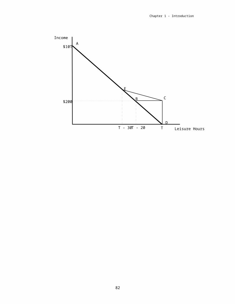
DMR

AC

MC

Q1 QQ*

P1

P2

Q2


5. An unregulated, profit-maximizing natural monopolist will produce Q1 units of output and charge a price per unit equal to P1. Since price is greater than marginal cost, the monopolist’s output is inefficient. The efficient level of output is Q*, where price equals marginal cost. Excess burden is the area between the demand curve and the marginal cost curve between output levels Q1 and Q*.

If the firm is required by law to charge average cost, then price will be P2 and the firm can break even by producing Q2 units of output. Q2 is below Q*, so although average cost pricing leads to more output than at the profit-maximizing level, it still falls short of the efficient amount and there is still an excess burden, measured as the area between the demand curve and the marginal cost curve between output levels Q2 and Q*.

6. The marginal benefit of underreporting is equal to the taxes saved, which is simply the person’s marginal tax rate, or MB = t. The expected marginal cost of underreporting $1 of income is equal to the product of the probability of getting caught and the fine per dollar of underreporting, or MC = ρ*Marginal Penalty. The optimal amount of underreporting, R* equals zero if MC ≥ MB. Thus, if ρ*Marginal Penalty ≥ t, then there will be no underreporting. With ρ = 0.02 and t = 0.35, the inequality becomes 0.02*Marginal Penalty ≥ 0.35, or Marginal Penalty ≥ $17.50. With a fine of $17.50 (or more), Sharlene would not cheat on her taxes.

82


7. The problem with a one-time tax on profits is that the government has an incentive to renege on its promise. The time inconsistency of optimal policy occurs when the government cannot implement an optimal tax policy because the stated policy is inconsistent with the government’s incentives over time. Since pharmaceutical companies know that government has an incentive to impose a tax on profits more than once, their behavior will be affected by the tax, creating an excess burden.

8. a. It is true that a proportional tax on all commodities (including leisure) is equivalent to a lump sum tax. To illustrate, consider the simplest example where there are only two goods: consumption goods and leisure. The budget constraint is equal to: pCC+wL=I, where pC and w are the prices of consumption goods and leisure, C and L are the quantities of consumption and leisure, and I is income. Then a proportional tax on all goods changes the budget constraint to: (1-τ)pCC+(1-τ)wL=I, or rearranging, pCC+wL=I’, where I’=I/(1-τ)<I. Thus, a proportional tax on all goods does not change relative prices and is equivalent to taking away income. So it is equivalent to a lump sum tax.

b. It is (usually) false that efficiency is maximized when all commodities are taxed at the same rate; this will not be true if leisure is untaxed. Imagine a more complicated budget constraint: pCC+pFF+wL=I. If leisure cannot be taxed, then a tax on commodities leads to a budget constraint of (1-τ)pCC+(1-τ)pFF+wL=I, which does change the relative price of leisure compared with food or consumption goods. Thus, it is not a lump sum tax. Instead, the inverse elasticity rule given in equation (16.9) would suggest that the ratio of the tax rates are inversely related to the ratio of the compensated demand elasticities for all commodities that can be taxed. That is, (tC/tF)=(ηF/ηC).

c. It is true that average cost pricing for a natural monopoly allows the enterprise to break even, but the outcome is inefficient. Figure 16.3 in the textbook shows the typical natural monopoly problem, with an initial fixed cost, and an ever-declining marginal cost curve. In this case, the average cost curve is always declining, but above the marginal cost curve. Setting P=AC results in an output level of ZA and zero economic profits. The figure illustrates, however, that the marginal benefit of more output exceeds the marginal cost, so the efficient level of production occurs at P=MC, or an output level Z*>ZA. The deadweight loss is the area between the demand curve DZ and marginal cost curve, going from ZA to Z*. If output were at the efficient level, however, there would be economic losses rather than zero profits.

d. One notion of horizontal equity is that people in equal positions should be treated equally by the tax system. Under this traditional notion of horizontal equity, the fact that Tom’s workplace provides free access to a fitness room suggests this kind of compensation should be taxed; Jerry pays “full taxes” on his compensation while Tom does not. Another notion of horizontal equity relies on the utility definition of horizontal equity. This concept says that if two individuals have the same utility without taxes, they should have the same utility with taxes,

83


and the taxes should not affect the utility ordering. One implication of the utility definition is that any existing tax structure does not violate the notion of horizontal equity if individuals are free to choose their activities and expenditures. If Tom and Jerry have free choice between the two different jobs (and identical preferences), then the net after-tax rewards (including amenities) must be the same at both jobs; otherwise there would be migration. In this case, the before-tax wage on Tom’s job adjusts for the fact that there is a fringe benefit.

84


Chapter 17 – The Personal Income Tax

1. The Haig-Simons definition of income is the net change in the individual’s power to consume during a given period. This criterion suggests the inclusion of all sources of potential increases in consumption and also implies that any decreases in an individual’s power to consume should be subtracted in determining income. Overall, it reflects the broadest possible base of income. Allowing capital losses of $5,000 to be deductible against other forms of income, rather than the current $3,000, would move the tax system more in the direction of the Haig-Simons criterion.

2. Personal fitness expenses should be counted as income according to the Haig-Simons definition, since they represent a net increase in the individuals power to consume. It would be difficult to devise a consistent system for determining whether such benefits should be taxable since the availability of personal fitness equipment does not prove that the individual used the equipment. It would also be difficult to accurately measure the value of such consumption.

3. Suppose Jones buys the oil stock for $1,000 at the start of period 0. At the start of period 1, he has two options.

a. Hold the oil stock one more period, then sell.

b. Sell the oil stock, buy the gold stock and hold it for one period.In both cases, it is assumed that all assets are sold, and any taxes paid at the end of period 2. What are the returns to option a)? At a 10 percent rate of appreciation, the oil stock is worth $1,210 after period 2, the capital gain is $210 and assuming a 29 percent rate applies to capital gains, the capital gains tax is 28 percent of $210 or $58.80. Thus, Jones is left with $1,210 - $58.80 or $1,151.20 after tax.

If Jones follows strategy b), the value of the oil stock at the start of period 1 is $1,000, the capital gain is $100, and the tax $28. Thus Jones has $1,672 left over to proceeds (V) from selling the gold stock at the end of period 1.

V = Value of gold stock – taxes= (1+r)($1,072) –(.28)[(1+r)($1,072)-($1,072)]= (1+r)($1,072) –(.28)r($1,072)= $1,072 + .72r($1,072)

Setting V = $1,151.20 (same as oil stock):$1,151.20 = $1,072 + .72r($1.072) r=10.26%

Thus the gold stock must pay a “premium” of 0.26% (10.26% - 10%) over the oil stock in order to overcome the tax cost of realizing the capital gain.

85


4. If same-sex couples were allowed to legally marry, they would be subject to the marriage penalty, resulting in an increase in income tax revenues.

5. For an itemizer, a $500 tax deduction lowers the tax bill by t*deduction. Thus, for an itemizer with a 30% marginal tax rate, the tax bill is lowered by 30%*$500, or $150. A (refundable) tax credit, on the other hand, directly lowers the tax bill by that amount, in this case, $500.

6. a. With a tax rate of t=0.3, and a nominal interest rate of i=0.13, the nominal after-tax rate of interest is (1-t)i=(1-0.3)0.13=0.091. With an expected inflation rate of π=0.08, the real after-tax rate of interest is (1-t)i-π=(1-0.3)0.13-0.08=0.091-0.08=0.011.

b. If the expected inflation rate increased by 3 percentage points to π=0.11, and the nominal interest rate also increases by 3 percentage points to i=0.16, then the real after-tax rate of interest is now (1-t)i-π=(1-0.3)0.16-0.11=0.112-0.11=0.02. The real after-tax rate of return falls from 1.1% to 0.2%. This is because the tax system taxes nominal, not real, returns.

c. In general, consider two rates of inflation, π<π’. The key question is when taxes are present, by how much must the nominal interest rate increase in order to have the same real rate of return. This is calculated by equating real rates of return under different inflation rates (holding constant taxes): (1-t)i-π=(1-t)i’-π’. One can rearrange this equation: (π’-π)=(1-t)(i’-i), or (i’-i)= (π’-π)/(1-t). This can in turn be expressed as: Δi=Δπ/(1-t). Intuitively, the left-hand side of this final equation is the change in nominal interest rates that keeps the real after-tax rate of interest unchanged. It is equal to the change in the expected inflation rate divided by (1-t). Thus, returning to part 6b, for a 3 percentage point change in the inflation rate and a marginal tax rate of t=0.30, nominal interest rates would have to increase by approximately 4.3 percentage points.

7. Much of the public debate concerning the marriage tax focuses on whether it is fairer to tax individuals or families. Beliefs concerning the choice of the fairest taxable unit are influenced by value judgments and by attitudes toward the role of the family in society. Nobel laureate Ed Prescott suggests that the design of the tax system should avoid using the tax system to either encourage or discourage marriage, whenever possible.

8. The Haig-Simons definition of income provides no rationale for reducing the tax rates on certain types of income. Some economists hope that reduced tax rates on dividends, capital gains, and labor income will strengthen incentives to work, save, and invest. Others are not convinced, and there are many arguments on both sides of the issue.

86


9. a. i. A family of four would receive four exemptions that totaled $13,200 (4*$3,300) in 2006.

ii. Ignoring other features like the exemption phaseout, an increase in income of $2,500 leads to an increase in taxes of $875 with a marginal tax rate of 35% ($875=$2,500*35%).

iii. Personal exemptions are reduced by 2 percentage points for each $2,500 increase in AGI. Thus, the exemption falls from $13,200 to 98%*$13,200, and taxable income goes up by 2%*$13,200, or $264.

iv. The additional increase in taxable income of $264 increases the tax liability by 35%*$264, or $92.40.

v. The total change in tax liability, the effective tax rate, is ($875+$92.40)/$2,500, or 38.696%.

b. i. With an extra $100 in income, the family would owe an additional 35%*$100, or $35 in taxes.

ii. Otherwise allowable itemized deductions are reduced by 2 percent of the amount by which AGI exceeds $150,500. However, the reduction cannot be more than 80 percent of the total of itemized deductions. An additional $100 in AGI may reduce itemized deductions by $2 if AGI exceeds $150,500. This would mean an increase in taxable income of $102.

iii. Assuming the additional income caused allowable itemized deductions to fall by $2, the family’s tax liability increased by 35%*$102, or

$35.70.

iv. The effective tax rate is ($35.70)/$100=35.7%.

10. Of the $4,000 of earnings that Sam has, he is able to invest (1-t I)*earnings in the market, or (1-0.25)*$4,000=$3,000. Assume that when he saves the money in a taxable account, he has to pay taxes each year on the capital gains, and that those capital gains are treated as ordinary income and taxed at 25%. In this case, his after-tax rate of return is (1-t I)*r, or (1-0.25)*8%, or 6%. Thus, after 10 years of investment, the amount of money in the taxable savings account is $3,000*(1.06)10=$5,372.54. If he invests the money in a Roth IRA, the money accrues at the before-tax rate of return, and there is no tax liability at the end. Thus, the amount in the Roth IRA is $3,000*(1.08)10=$6,476.77. It turns out that the key difference between a traditional IRA and a Roth IRA is whether the income tax rate today differs from the income tax rate in retirement. Thus, the amount in the Roth IRA would be identical to that of a traditional IRA if tax rates 10 years from now were the same 25%.

87


Chapter 18 – Personal Taxation and Behavior

1. The supply of labor (and other factors) in and out of a city is more elastic than the supply of factors to the nation as a whole. Therefore, an income tax reduction at the city level is likely to lose less revenue than such a reduction at the federal level, ceteris paribus. Just as one can think of “welfare-induced” migration for poor households, one can think of “tax-induced” migration for businesses and possibly workers. If the city lowers tax rates (and other cities do not respond accordingly), then one imagines that a number of businesses will enter that state and spur economic activity.

2.

If individuals view their loss in the labor income taxes as offset by the benefits of public services, labor supply falls by AB hours. This is the compensated change in hours with respect to a change in the net wage rate.

3.

88


4. The effect of the change in the highest marginal tax rate on the individual’s budget constraint is demonstrated below:

Income

Leisure

The resulting change in the tax rate moves part of the budget line out to the new, dotted budget constraint. This policy has an effect on labor supply analogous to the effect of an increase in an individual’s wage rate on labor supply: it is theoretically ambiguous. The reason for this ambiguity is that there are two competing effects -- a substitution effect which acts to decrease leisure, and an income effect which increases leisure. The decrease in the tax rate makes leisure more expensive, so the substitution effect dictates that less of it is to be consumed. However, there is extra income provided by this tax cut, and the income effect makes the individual want to consume more leisure. These two competing effects make the overall change in labor supply ambiguous. Existing empirical work suggests that for prime age males, the income and substitution effects more or less cancel each other out. For working wives, the substitution effect dominates, meaning that the reduction in marginal tax rates would tend to increase their labor supply.

The effect on savings can be demonstrated using a diagram illustrating the change in the intertemporal budget constraint that results from this tax change:

FutureConsumption

E E’ Current Consumption

The policy moves the endowment point from point E to E’, and it changes the slope of the intertemporal budget constraint, which is equal to [1 + (1-t)r], where “t” is the tax rate, and “r” is the real interest rate. Once again, the overall effect of this policy on

89


savings will be ambiguous, since there are again competing income and substitution effects. The extra income gained from the tax cut will make this individual want to opt for more consumption in both periods (now and in the future), so this will cause savings to increase (intuitively, the individual will consume some of her extra income now, and some in the next period). However, the tax cut will also change the slope of the budget line. This causes a substitution affect which makes consuming in the current period more expensive (so savings will increase), but it causes income to rise, which makes this individual want to consumer more in the current period. The counteracting effects make it difficult for us to say what will happen to overall savings. Econometric work suggests that changes in marginal tax rates have little effect on individual saving.

Lastly, the effect on tax revenues will be negative (a decrease in the tax rate will have a direct effect in this case). However, this decrease will not be as pronounced as we might think. First, to the extent that some individuals work more, taxable income will increase. More importantly, individuals will opt for more taxable income instead of nontaxable income as the tax rate falls. For instance, since fringe benefits are like non-taxable income, an individual will prefer them to cash payments (which are taxable) when the tax rate is high. However, the opposite is true when the tax rate falls. Thus, although with a lower tax rate less revenue is collected from a given tax base, this decrease is somewhat counteracted by the increase in the base itself. That said, there is no evidence that the increase in the base would be large enough to make the tax self-financing.

5. The interest rate cut may be successful at stimulating consumer spending. Reducing the rate of return on savings reduces the opportunity cost of current consumption, which tends to increase current consumption and lower saving (the substitution effect). On the other hand, the fact that the interest rate is lower makes it harder for a saver to achieve any future consumption goal (the income effect), so the effect may be to increase saving and reduce current consumption. The policy will have the desired results if the substitution effect dominates the income effect.

6. Increasing tax rates will not increase tax revenue if European tax rates are on the right-hand side of the Laffer Curve (Figure 18.6), where the tax rate exceeds tA.

7. A rational person will increase savings in reaction to reduced interest rates, as suggested by the financial columnist, if the income effect is stronger than the substitution effect. This would result in a downward-sloping supply of savings curve.

8. The individual receives a benefit equal to the market rental value of the house because he lives in the house. Whether he lives in the house or not, he receives a net benefit; the only difference is that when he rents out the house, he explicitly receives the rent in cash, while if he lives in the house, he effectively pays himself. Implicit or not, it is still income, and under a Haig-Simons income tax, it should be taxed.

90


9. a. The supply curve is given by S = -100 + 200wn. The gross wage is w = 10, and the net wage is wn = (1-t)w = (1-t)10. The difference, then, between the gross and net wage for any tax rate is w - wn = 10t. This is the tax collected per hour of work.

The tax revenue for any given hours of work is then the product of the tax collected per hour of work and the labor supply curve:

tax revenue = 10t*(-100+200(1-t)10) = -1,000t + 20,000t -20,000t2

= 19,000t - 20,000t2

The tax rate t = 0.7 is beyond the revenue maximizing point (this can be shown by computing tax revenue for a slightly lower tax rate, like t=0.69.

b. Taking the derivative:

dTax Revenue/dt=0

yields 19,000-40,000t=0, or

t = (19,000/40,000), or

t = 0.475 as the revenue maximizing tax rate.

91


Chapter 19 – The Corporation Tax

1. A corporation may use retained earnings to increase dividends, but shareholders pay additional income taxes as a result. Even though the franchises weren’t particularly profitable, it may have been in the shareholders’ best interest to purchase them instead of paying additional dividends.

2. a. The real value of depreciation allowances, of equation (19.1), falls.

b. When falls, the user cost of capital increases.

c. Index appreciation allowances.

3. If the $20 million is expensed, the firm gets a deduction of $20 million in the current year. If the $20 million is depreciated, the deductions are spread over time (in a way that depends on the specifics of the depreciation schedule). The present value of the future flow of deductions is less than $20 million. Because the package design will yield benefits that extend over a period of time, it would seem sensible to view it as a capital expenditure. If so, depreciation is appropriate, and the IRS was right.

4. The user cost of capital, C, in Equation 19.4 is:

C = (r + )/[(1 - )x(1 – t)]

Where t is the individual tax rate on dividend income. Suppose Lee Enterprises can lend their money out and receive an after-tax rate of return of 10 percent. Assume that they could also buy a new printing press that would experience economic depreciation of 2 percent annually. Ignoring taxes, the printing press would have to generate a 12 percent return to cover depreciation. If the corporate tax rate is 35 percent and the marginal rate on dividends is 20 percent, the printing press would have to earn a before-tax return of 23.07 percent to give Lee Enterprises the same after-tax return as lending money at 10 percent. Reducing the marginal rate on dividends lowers the necessary rate from 23.07 percent to 21.7 percent, therefore making it more likely that the purchase of a new printing press would be a profitable investment. If Lee Enterprises did not immediately buy more presses, this does not prove that the lower tax on dividends had no effect, but does imply that reducing the user cost from 23.07 percent to 21.7 percent was not enough to justify this particular investment.

5. This statement assumes that the corporate tax is equivalent to an income tax. Table 14.2 shows that a proportional tax on both capital and labor is equivalent to an income tax. Thus, the statement assumes that the corporate tax is a proportional tax on both capital and labor.

92


6. A retroactive rebate of the alternative minimum tax for corporations would simply be a lump sum transfer. Thus, according to neoclassical theory, such a rebate would not have an effect on investment, because it does not affect the user cost of capital. The user cost of capital depends on current individual and corporate tax rates, after-tax rates of return in the capital market, economic depreciation, depreciation allowances, and investment tax credits. None of these is affected by the AMT rebate described in the text. Moreover, because the firms involved in the AMT rebate were very large, it is hard to imagine that the rebate would relax liquidity constraints either.

7. O’Neill’s statement that, as chief executive of Alcoa, he “never made an investment decision based on the tax code,” is problematic for the shareholders of Alcoa. It makes no sense to ignore tax incentives when making business decisions; that is, after-tax returns are what matter. O’Neill’s lack of tax sophistication likely lowered the value of Alcoa relative to what it would have been had he taken account of the tax system.

8. The MIPS financial instrument, which could interchangeably be called debt or equity, would be attractive to a corporation because firms would want tax authorities to view the instrument as debt because the interest paid is tax deductible. On the other hand, firms want potential investors to view the instrument as equity, because more debt makes the firm a riskier investment. Although the tax law might be forced to view this MIPS instrument as debt, there is no reason why investors in the market (or credit rating agencies) would then view it as equity, however. In principle, investors and credit agencies should be able to see through such accounting gimmicks, though in practice, the accounting scandals showed that this was not the case.

9. The user cost of capital (ignoring depreciation allowances and investment tax credits) is given by equation (17.4) in the textbook, C=(r+δ)/[(1-θ)(1-t)], where r=after tax rate of return in the capital market, δ=economic depreciation, θ=corporate tax rate, and t=individual tax rate. Substituting the numbers from the problem into the formula, gives the user cost: C=(.08+.01)/[(.65)*(.7)]=.1978. Since the project’s return, 30%, is higher than this user cost of 19.8%, the company does invest in the project

93


Chapter 20 – Deficit Finance

1. a. The government borrowing to finance a Memorial Day parade increases the national debt. In designing an accounting system for the government, the borrowing in this case should, in fact, increase the national debt.

b. The sale of the Statue of Liberty to private entrepreneurs would decrease the national debt under current measurement. In the discussion on capital spending, the exercise here is similar to the sale of nondefense federal buildings in 2002. In designing an accounting system, this transaction is simply an exchange of assets and should have no effect on the debt, rather than decreasing the debt. The current system ignores tangible assets.

c. The law promising free (future) medical care to children under five affects future spending, not current spending. As such, it does not affect the current measurement of the debt. This is similar to the discussion of the implicit legislative promises about Social Security. In designing an accounting system, the present value of the entitlement should be counted as a current expense, so the debt should increase. The current system ignores implicit obligations.

d. The $100 tax would reduce the size of the national debt. The implicit promise to pay Lynne back $105 next year does not increase the size of the debt, assuming this is similar to the implicit promise to pay Social Security in the future. In designing an accounting system, again, this implicit promise should be counted. Assuming the present discounted value of the of the $105 paid back next year equals the $100 tax this year, then the impact on the debt should be zero, rather than to decrease it.

e. The $100 bond would increase the size of the national debt. The present value of these payments is the amount by which the bond contributes to the debt. In designing an accounting system for the government, the borrowing in this case should, in fact, increase the national debt.

2. Germany’s government owns tangible assets, including gold. Selling the gold might give the appearance of temporarily reducing the current year deficit, but is not a sensible long-term strategy.

3. The arrival of surpluses in the late 1990s, and the subsequent spending spree, are consistent with Milton Friedman’s view of deficits and government spending. His view is that, “What is predetermined is not spending but the politically tolerable deficits.” Since the deficit is fixed, increases in revenue lead to one-to-one increases in spending.

4. If the elasticity is zero, then taxing labor markets creates no distortion. But in the presence of taxes on capital income, crowding out in the capital market will generate an excess burden. Therefore, use tax finance.

94


5. Whether or not the burden of the debt is borne by future generations is controversial. One view is that an internal debt creates no net burden for future generations because it is simply an intragenerational transfer. However, in an overlapping generations model, debt finance can produce a real burden on future generations. The burden of the debt also depends on whether debt finance crowds out private investment. If it does, future generations have a smaller capital stock and, hence, lower real incomes, all other things equal. In a Ricardian model, voluntary transfers across generations undo the effects of debt policy, so crowding out does not occur.

6. The benefits-received principle, which states that the beneficiaries of a particular government spending program should pay for it, suggests that deficit finance is appropriate for war if the benefits are received by future generations. An efficiency standpoint would say that debt is appropriate if the expenditure is temporary, and there are not major pre-existing distortions in capital markets.

95


Chapter 21 – Fundamental Tax Reform: Taxes on Consumption and Wealth

1. a. The income tax is 50 percent, so Zach pays 50%*$10,000 = $5,000 in income taxes in the first period. In the second period, he earns $500 in interest (10% of savings = 10%*$5,000 = $500), so he pays taxes on interest of 50%*$500 = $250. The present value of Zach’s lifetime tax payments equals $5,000 + [$250/(1.1)] = $5,227.27.

b. In the second period, Zach has savings and interest equal to $5,500. He can consume $3,667 in period 2 and must then pay 50%*$3,667 = $1,833.50 in consumption taxes. The present value of Zach’s lifetime tax payments is then equal to $5,000 + [$1,833.50/(1.1)] = $6,667.

These calculations demonstrate the transitional problem in moving to a consumption tax because Zach had to pay high taxes during period 1 when he earned most of his income, and then had to pay high taxes during period 2 when he did his consuming.

2. The burden of the estate tax includes the resources used in estate planning and the effects of estate planning. Many families may alter their behavior in reaction to the estate tax and, if this results in less efficiency, the estate tax creates an excess burden that is not reflected by the number of taxable estates or the amount of tax revenue collected.

3. There is a fundamental confusion here. There is no reason to assume that the incidence of a general consumption tax (a VAT) will be the same as the incidence of a partial factor tax (corporate income tax).

4. a. For a fan giving a million-dollar ball to McGwire or Sosa, there would be a federal gift tax liability. Depending on the fan's circumstances, it could reach $150,000 or more. The person receiving the gift owes no tax.

b. If the fan keeps the ball, the fan would owe no tax now. But the ball would become part of his or her estate, taxable after death under the estate tax.

c. The fan can avoid tax entirely by giving the ball to a charity, since he could entirely deduct the value of the ball from his taxable income. The charity could sell the ball; the proceeds from the sale would not be taxed.

d. If the fan sells the ball, the fan owes tax on the net proceeds, just as the seller of any property would. The transaction would put the fan in the highest tax bracket, so that the marginal tax rate on the proceeds would be 39.6 percent.

e. If the fan holds onto the ball for a year, it becomes a long-term capital asset, subject to the maximum capital-gains tax rate of 28 percent. Unless the fan thinks that there is going to be a substantial drop in the market value of the ball, he or she should hold onto it for a year.

96


5. a. The expression “What you earn is what you keep” is false, because a consumption tax is equivalent to a tax on wages. The two are related by the expression (1+)=1/(1-t), where =consumption tax rate and t=income tax rate.

b. The expression, “Investment and savings would soar” may be true. A consumption tax raises the return to saving, but because of the conflict between income and substitution effects, one cannot know whether or not this will increase saving. Figures 18.9 and 18.10 in the textbook illustrate these possibilities.

c. The statement that “There is no evading the Fairtax” is false. Evasion can be a major problem with retail sales taxes, especially at high rates.

6. In the simplest possible case, the budget constraint is pC = wH, where p is the price of consumption, C is units of consumption, w is the wage rate, and H is hours of work. With an income tax, pC=(1-t)wH, where t=income tax rate. With a consumption tax, (1+)pC=wH, where =consumption tax rate. Thus, for any income tax rate t, we can find a consumption tax rate, , that is equivalent by solving the expression: (1+)=1/(1-t).

7. a. We can conclude that an income tax generates an excess burden if it creates a tax wedge between the amount a borrower pays and the amount a lender receives. With a 25% income tax and an interest rate of 8%, lenders receive (1 – t)r = 6%. Since interest paid is tax deductible, borrowers pay (1 – t)r = 6%. Therefore, there is no tax wedge and no excess burden.

b. If interest payments are not tax deductible, then borrowers pay 8%, while lenders receive 6% after taxes. Since there is a wedge between the two rates, the income tax creates an excess burden in this case.

c. If the income tax rate is t = 0.25, then (1+) = 1/(1-0.25) = 4/3, so the equivalent consumption tax is = 1/3. A consumption tax leaves unchanged the market rate of return because the receipt of interest income by itself does not create a tax liability. If interest payments are not tax deductible, there is no wedge between the rate lenders receive and the rate borrowers pay, so there is no excess burden.

d. If interest payments are tax deductible, then there is a wedge between the rate lenders receive and the rate borrowers pay, so the tax creates an excess burden. With a consumption tax rate of 1/3, borrowing $1 and paying 8% interest causes the tax liability to fall and the after-tax interest rate borrowers must pay is (1 – t)r = (2/3)0.08 = 5.36%. In this case, the wedge between the rate lenders receive (8%) and the rate borrowers pay (5.36%) is even larger than for a 25% income tax when interest payments were not tax deductible, so the excess burden is larger. Note that there is an excess burden associated with an income tax only when interest payments are not tax deductible, while there is an excess burden associated with a consumption tax only when interest payments are tax deductible.

97


8. Under an income tax, Amy's burden is $1,000*t in the first period, and .08($800)t in the second period (e.g., her investment income is taxed). Shirley's burden is identical in the first period, $1,000*t, but is lower in the second period, equal to .08($700)t. This is because Shirley consumed more in the first period and saved less. Thus, Amy has a higher lifetime tax burden because she has higher investment income. Under a proportional consumption tax, Amy and Shirley have the same lifetime tax burden, $1,000*, where is the consumption tax rate.

98


Chapter 22 – Public Finance in a Federal System

1. If there are inter-jurisdictional externalities, then gun control is a federal issue. For example, if lax gun control in one state leads to more crime in another state, there are inter-jurisdictional externalities.

2. Superficially, it seems a violation of horizontal equity for two people with identical properties to pay different taxes on them. However, the phenomenon of capitalization requires that we distinguish carefully between the owners at the time the tax is levied and the current owners. A property with an unduly high tax rate will sell for a lower price, other things being the same. Thus, a high tax rate does not necessarily make an individual who buys the property after the tax is imposed worse off. Indeed, equalizing assessment ratios could generate a whole new set of horizontal inequities.

3.

99


c.

4. Virtually all studies conclude that a dollar received by a community in the form of a grant results in greater public spending than a dollar increase in community income. This phenomenon has been dubbed the flypaper effect, because the money seems to stick in the sector where it initially hits.

5. The figure looks essentially like Figure 22.6 (without segment JH). What actually happens to spending on education depends on the income elasticity. The government need not increase spending on education by the full amount of lottery money collected because the rest of the state revenue is fungible. Thus, if previously 20 percent of general state revenue had been spent on education, after the lottery is implemented, perhaps only 17 percent of general state revenue is spent on education.

100


6. In the figure below, the (constant) marginal cost of hiring a firefighter is C. The demands for the two communities are D1 and D2. Suppose that initially the quantity is set at Q0. After decentralization, each community hires firefighters up to the point where the marginal benefit equals marginal cost, i.e., where their respective demand curves intersect C. This is at Q1 for community 1 and Q2 for community 2. Community 1 gains abc. Community 2 gains dbe. Community 1 gains more because its demand curve is more inelastic.

7. The “user-fee” view of property taxes regards property taxes as payment for local public services. The statement “its presence would raise property values and the extra tax revenues would easily repay the construction costs” reflects this view -- that people pay for the recreational services made available by the part with their property taxes. The statement is not consistent with the “traditional view” or the “new view,” both of which ignore the local services aspect.

8. Originally, the effective state price of $1 spending on welfare recipients was $0.50 with a one-for-one federal match rate. If the federal match rate changes to two-for-one, the effective state prices of $1 spending falls to $0.33, or a 34 percent change in the price. Using Baicker’s (2001) elasticity estimate of 0.38, a 34 percent change in price should increase state spending by 12.92% (=0.38*34%).

101


102

Documents

Answer to end of chapter solution