Embed Size (px)
Citation preview
SELECTED ANSWERS
Chapter 1: What Is Statistics
1.1 a. The population of interest is the weight of shrimp maintained on the specific diet fora period of 6 months.
b. The sample is the 100 shrimp selected from the pond and maintained on the specificdiet for a period of 6 months.
c. The weight gain of the shrimp over 6 months.
d. Since the sample is only a small proportion of the whole population, it is necessary toevaluate what the mean weight may be for any other randomly selected 100 shrimps.
1.5 a. All football helmets produced by the five companies over a given period of time.
b. The 540 helmets selected from the output of the five companies.
c. The amount of shock transmitted to the neck when the helmet’s face mask is twisted.
d. The neck strength of players is extremely variable for high school players. Hence, theamount of damage to the neck varies considerably from player to player for exactlythe same amount of shock transmitted by the helmet.
Chapter 2: Using Surveys and Scientific Studies to Gather Data
2.1 The relative merits of the different types of sampling units depends on the availability ofa sampling frame for individuals, the desired precision of the estimates from the sample tothe population, and the budgetary and time constraints of the project.
2.3 A more precise estimate can be obtained by considering individual cars but it may be verydifficult obtaining the sampling frame. By selecting parking lots and examining all cars inthe lot, the data is more easily obtained but the individual cars in the lot may have commoncharacteristics reflecting the set of persons using the parking lot. Thus, the cars in the lotare a cluster sample and not a simple random sample. This results in a less precise estimateof the population than examining the same number of cars selected individually.
1
2.5 The agency could stratified farms based on the total acreage of farms in the state. A simplerandom sample of farms could then be selected within each strata and a questionaire sentto the farmer.
2.9 a. No. The survey in which the interviewer showed the peanut butter should be themore accurate because it does not rely on the respondent’s memory of which brandwas purchased.
b. Both surveys may have survey nonresponse bias because an entire segment of thepopulation (those not at home) cannot be contacted. Also, both surveys may haveinterviewer bias resulting from the way the question is posed (e.g., tone of voice). Inthe first survey, results may be biased by the respondent’s ability to recall correctlywhich brand was purchased. The second survey may be biased by the respondent’sunwillingness to show the interviewer the peanut butter jar (too intrusive), or by therespondent not recognizing that the peanut butter that had purchased was low fat.
2.11 a. ”Employee” should refer to anyone who is eligible for sick days.
b. Use payroll records. Stratify by employee categories (full-time, part-time, etc.), em-ployment location (plant, city, etc.), or other relevant subgroup categories. Considersystematic selection within categories.
c. Sex (women more likely to be care givers), age (younger workers less likely to haveelderly relatives), whether or not they care for elderly relatives now or anticipate doingin the near future, how many hours of care they (would) provide (to define ”substan-tial”), etc. The company might want to explore alternative work arrangements, suchas flex-time, offering employees 4 ten-hour days, cutting back to 3
4 -time to allow moretime to care for relatives, etc., or other options that might be mutually beneficial andprovide alternatives to taking sick days.
2.13 If phosphorus first: [P,N]
[10,40], [10,50], [10,60], then [20,60], [30,60]
Or [20,40], [20,50], [20,60], then [10,60], [30,60]
Or [30,40], [30,50], [30,60], then [10,60], [20,60]
If nitrogen first: [N,P]
[40,10], [40,20], [40,30], then [50,30], [60,30]
Or [50,10], [50,20], [50,30], then [40,30], [60,30]
Or [60,10], [60,20], [60,30], then [40,30], [50,30]
2
Chapter 3: Data Description
3.1 a. Pie Chart
b. Bar Graph
3.3 Pie Chart and Bar Graph should be plotted. Pie chart is better since we are proportionallyallocating the food dollar to seven categories.
3.9 The relative frequency histogram is multimodal, skewed to the right.
3.11 stem-and-leaf
Stem-and-Leaf Plot (Leaf Unit 100)
2 70,71,983 59,60,824 51,67,88,985 12,20,61,726 34,43,867 849 47,8613 0516 8224 7049 04
3.13 a. Construct separate relative frequency histograms.
3.25 Mean = 15.2, Median = 14.5, Mode = 18
3.27 10% Trimmed Mean = 14.83.
3.29 mean ≈ 7.6 mode ≈ 7
median ≈ 7.4
3.31 a. The mean cannot be approximated. Mode ≈ 240.
median ≈ 219.2
b. The median
3.33 a. Mean = 46.3 and Median = 29.
b. The median would be unchanged but the mean would increase
3.35 a. The rounded measurements:
3
2.10 2.80 2.17 1.99 2.22 3.092.40 2.50 2.80 2.10 2.92 2.201.70 2.70 2.82 2.67 3.05 2.932.90 1.90 2.38 2.65 2.77 1.851.60 2.70 2.68 2.06 2.36 2.282.70 2.40 2.39 2.55 1.80 1.96
b. Sample modes = 2.10, 2.77, 2.82
c. Median = 2.45
d. Mean = 2.43
3.37 a. The values are given below:
Group Mean Median Mode
I 2.923 2.805 no modeII 1.592 1.565 1.55, 1.57III 0.797 0.755 0.70
b. mean = 1.7707 median = 1.565 mode = 0.70, 1.55, 1.57
3.39 a. X = 5. Yes.
b.∑8i=1(yi − 5)2 = 46
c. s = 2.56 CV = 51%.
3.41 Age: s ≈ 2.
Experience: s ≈ 5.25.
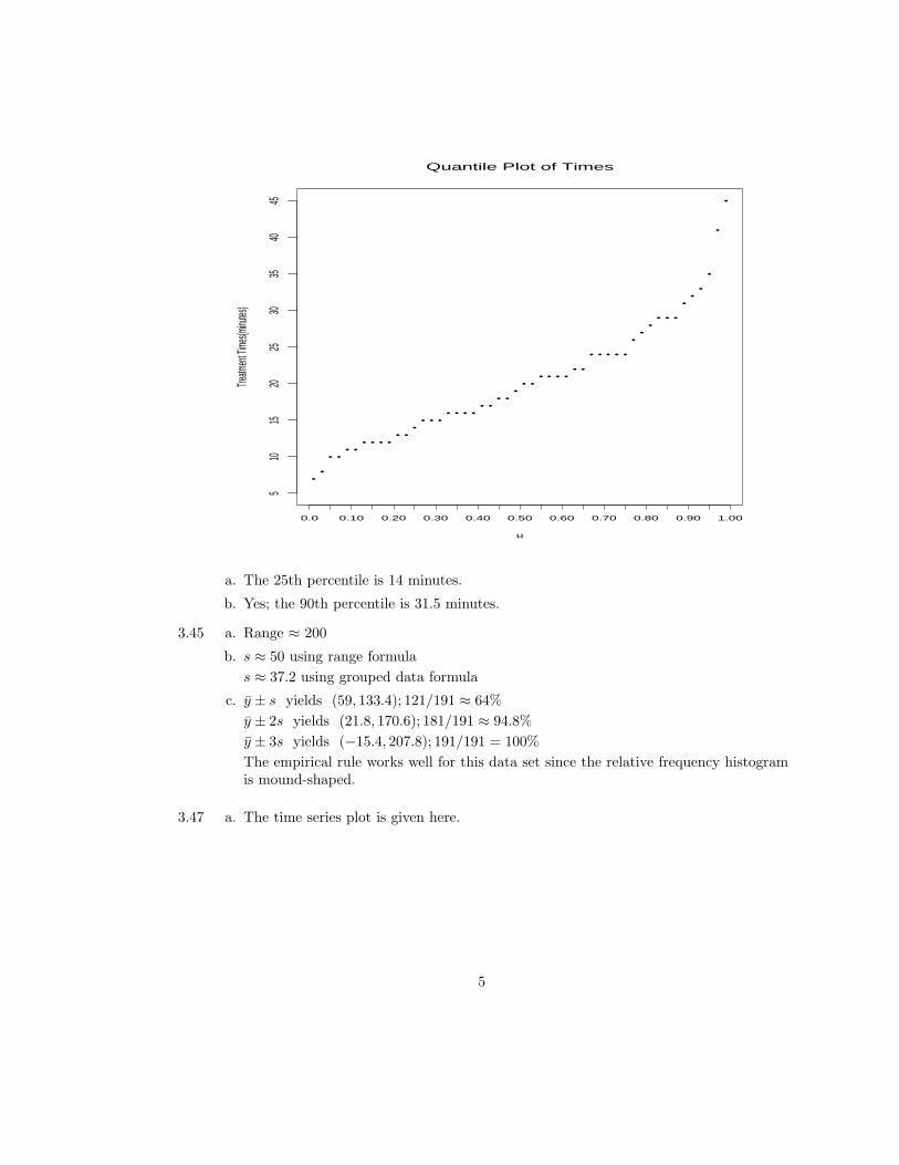
3.43 The quantile plot is given here.
4
••
• •• •
• • • •• •
•• • •
• • • •• •
• ••
• •• • • •
• •
• • • • •
••
•• • •
••
•
•
•
•
Quantile Plot of Times
u
Treatm
ent T
imes(m
inutes
)
0.0 0.10 0.20 0.30 0.40 0.50 0.60 0.70 0.80 0.90 1.00
510
1520
2530
3540
45
a. The 25th percentile is 14 minutes.
b. Yes; the 90th percentile is 31.5 minutes.
3.45 a. Range ≈ 200
b. s ≈ 50 using range formula
s ≈ 37.2 using grouped data formula
c. y ± s yields (59, 133.4); 121/191 ≈ 64%
y ± 2s yields (21.8, 170.6); 181/191 ≈ 94.8%
y ± 3s yields (−15.4, 207.8); 191/191 = 100%
The empirical rule works well for this data set since the relative frequency histogramis mound-shaped.
3.47 a. The time series plot is given here.
5

Mercury Concentration (ng/g dry weight)
Year
Mercu
ry Co
ncentr
ation
1969 1971 1973 1975 1977 1979 1981 1983 1985 1987 1989 1991
010
020
030
040
050
060
070
0
Site 1Site 2
b. Site 1: Median = 18.25, Mean = 29.18
Site 2: Median = 184.1, Mean = 287.1
c. Site 1: s = 26.95, CV = 92%
Site 2: s = 194.7, CV = 68%
d. No, Site 1 does not have values for these years.
3.49 Q2 = 20 Q1 = 17.5, Q3 = 23.5
3.50 a. Stem-and-Leaf Plot is given here:
Stem Leaf
2 52 6772 93 001113 2233333 53 673 8
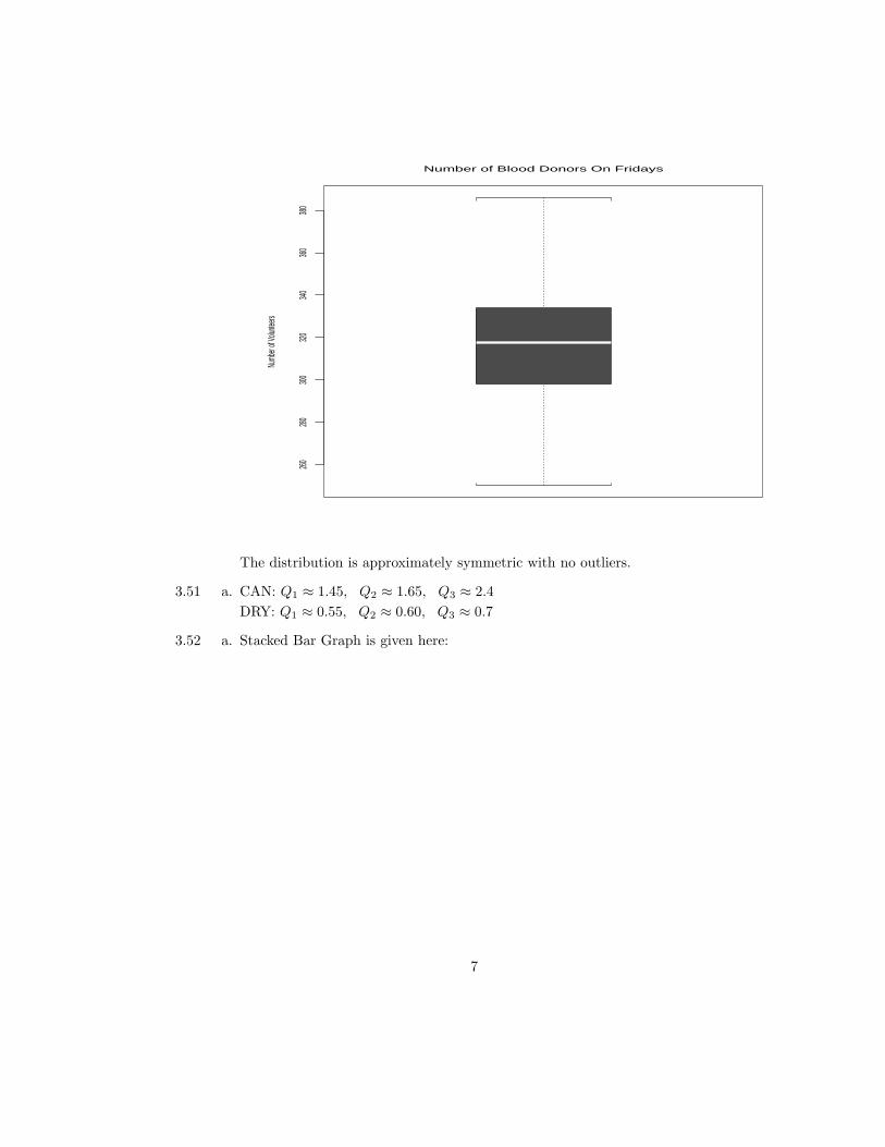
b. Min=250, Q1 = 298, Q2 = 317.5,
Q3 = 334, Max=386
6
260
280
300
320
340
360
380
Number of Blood Donors On Fridays
Numb
er of
Volun
teers
The distribution is approximately symmetric with no outliers.
3.51 a. CAN: Q1 ≈ 1.45, Q2 ≈ 1.65, Q3 ≈ 2.4
DRY: Q1 ≈ 0.55, Q2 ≈ 0.60, Q3 ≈ 0.7
3.52 a. Stacked Bar Graph is given here:
7

MiddlePrimaryIllerate
Shifting Settled TownDweller
020
4060
8010
012
014
016
018
020
0
Literacy Level of Three Subsistence Groups
Subsitence Group
Perce
nt in
Litera
cy Le
vel
b. Illiterate: 46%, Primary Schooling: 4%, At Least Middle School: 50%
Shifting Cultivators: 27%, Settled Agriculturists: 21%, Town Dwellers: 51%
3.53 50% of workers who resign are in the youngest age group; of those who transfer, 68.2% arein their 30’s; and of those who either retire or got fired 86.24% are at least 40 years old.
3.55 a. The means and standard deviations are given here:
Supplier y s
1 189.23 2.962 156.28 3.303 203.94 8.96
b. Side-by-side Boxplots are given here:
8

150
155
160
165
170
175
180
185
190
195
200
205
210
215
220
Supplier 1 Supplier 2 Supplier 3
Deviations from Target Power Value for Three Suppliers
Supplier
Devia
tions fr
om Ta
rget
d. Supplier 2
3.57 A time series plot with M2 and M3 values on the vertical axis and months on the horizontalaxis is given here.
9

Money Supply (Trillions of Dollars)
Month
Mone
y Sup
ply
1 2 3 4 5 6 7 8 9 10 11 12 13 14 15 16 17 18 19 20
2.02.1
2.22.3
2.42.5
2.62.7
2.82.9
3.03.1
3.23.3
3.43.5
M2M3
3.59 a. mode = 5, median = 15, mean = 15.96
b. range = 30, s ≈ 7.5
c. s = 8.5
d. No, the histogram for the data set is skewed to the right and hence is not mound-shaped.
3.63 a. Mean = 0.65; Median = 0.55; Mode = 0.5
b. Mean = 1.21; Median = 0.55; Mode = 0.5
The mean increases but the median and mode remain the same.
3.65 b. Highly skewed to the right
c. 1424± 3488⇒ (-2063, 4912) contains 37/41 = 90.2%
1424± (2)3488⇒ (-5551, 8400) contains 38/41 = 92.7%
1424± (3)3488⇒ (-9039, 11888) contains 39/41 = 95.1%
These values do not match the percentages from the Empirical Rule: 68%, 95%, and99.7%.
d. 1.48± 1.54)⇒ (-0.06, 3.02) contains 31/41 = 75.6%
1.48± (2)1.54⇒ (-1.60, 4.56) contains 40/41 = 97.6%
1.48± (3)1.54⇒ (-3.14, 6.10) contains 41/41 = 100%
These values closely match the percentages from the Empirical Rule: 68%, 95%, and99.7%.
10
3.67 a. There has been very little change from 1985 to 1996.
b. Yes
c. No
d. The cost of homes is very high.
3.69 a. Mode = 2.5 Median ≈ 7.04
b. Mean ≈ 8.3
c. median
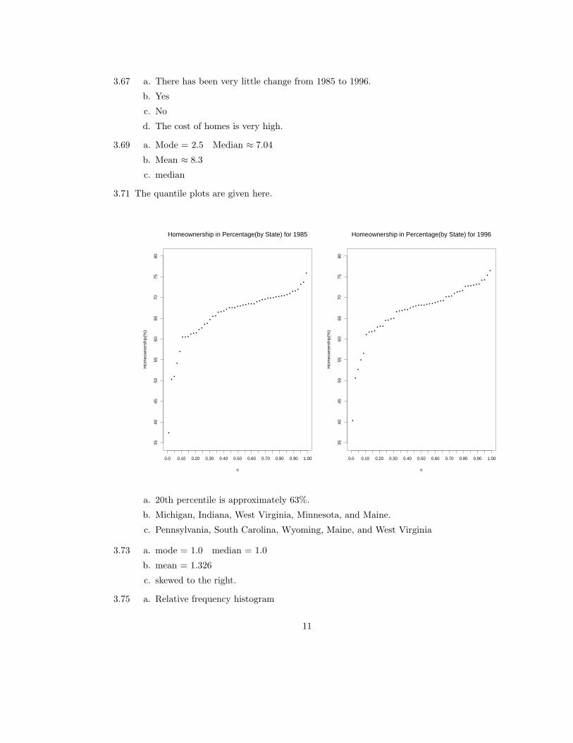
3.71 The quantile plots are given here.
•
••
•
•
• • • • • •• •
• ••
• •• • • • • • • • • • • • • • • • • • • • • • • • • • • • • •
• •
•
Homeownership in Percentage(by State) for 1985
u
Hom
eow
ners
hip(
%)
0.0 0.10 0.20 0.30 0.40 0.50 0.60 0.70 0.80 0.90 1.00
3540
4550
5560
6570
7580
•
•
•
•
•
• • • •• • •
• • • •
• • • • • • • • • • • • • • • • • •• • • • • • •
• • • • • •• •
••
Homeownership in Percentage(by State) for 1996
u
Hom
eow
ners
hip(
%)
0.0 0.10 0.20 0.30 0.40 0.50 0.60 0.70 0.80 0.90 1.00
3540
4550
5560
6570
7580
a. 20th percentile is approximately 63%.
b. Michigan, Indiana, West Virginia, Minnesota, and Maine.
c. Pennsylvania, South Carolina, Wyoming, Maine, and West Virginia
3.73 a. mode = 1.0 median = 1.0
b. mean = 1.326
c. skewed to the right.
3.75 a. Relative frequency histogram
11

b. Mean ≈ 109.6
s ≈ 31.106
3.77 a. Plot relative frequency histogram.
b. 1100
c. mean = 1091.96, median = 1039
d. skewed to the right.
3.79 The stem-and-leaf diagram is given here:
Stem Leaf
54 75556575859606162 563 06465 666 4 7 767 7968 8 88 8869 1 4 7 970 0 1 2 333 871 1
left skewed.
3.81 Summary table
Number of Members Mean Median
1 93.75 78.52 98.652 953 113.3125 1004 124.857 112.5
5+ 131.90 128.50
3.83 a. New policy y = 2.27, s = 3.26
Old policy: y = 4.60, s = 2.61
3.85 b. Plants: y = 677794.60
Arrests:y = 95
10% trimmed mean:
Plants: y = 142327.64
Arrests: y = 59.7
12
20% trimmed mean:
Plants: y = 133039.33
Arrests: y = 41.30
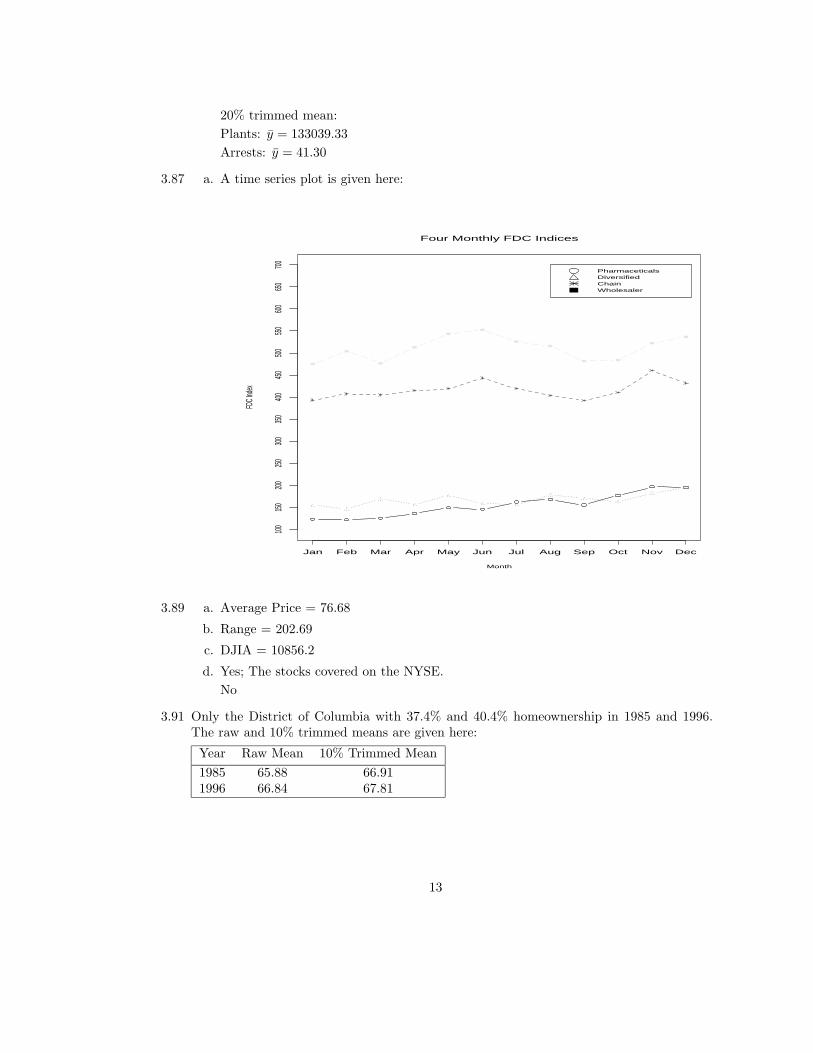
3.87 a. A time series plot is given here:
Four Monthly FDC Indices
Month
FDC I
ndex
100
150
200
250
300
350
400
450
500
550
600
650
700
Jan Feb Mar Apr May Jun Jul Aug Sep Oct Nov Dec
PharmaceticalsDiversifiedChainWholesaler
3.89 a. Average Price = 76.68
b. Range = 202.69
c. DJIA = 10856.2
d. Yes; The stocks covered on the NYSE.
No
3.91 Only the District of Columbia with 37.4% and 40.4% homeownership in 1985 and 1996.The raw and 10% trimmed means are given here:
Year Raw Mean 10% Trimmed Mean
1985 65.88 66.911996 66.84 67.81
13

Chapter 4: Probability and Probability Distributions
4.1 a. Subjective probability
b. Relative frequency
c. Classical
d. Relative frequency
e. Subjective probability
f. Subjective probability
g. Classical
4.3 Using the binomial formula, the probability of guessing correctly 15 or more of the 20questions is 0.021.
4.5 HHH, HHT, HTH, THH, TTH, THT, HTT, TTT
4.7 a. P(A)
= 58
P(B)
= 18
P(C)
= 78
b. Events A and B are not mutually exclusive
4.9 Because P (A|B) = 37 6= 3
8 = P (A)⇒ A and B are not independent.
A and C are not independent.
B and C are not independent.
4.11 A and B are not independent.
A and C are not independent.
A and D are not independent.
B and C are independent.
B and D are not independent.
C and D are not independent.
None of the pairs of the events are mutually exclusive.
4.13 No
4.15 a. A: Generator 1 does not work
b. B|A: Generator 2 does not work given that Generator 1 does not work
c. A ∪B: Generator 1 works or Generator 2 works or Both Generators work
4.17 a. S = {F1F2, F1F3, F1F4, F1F5, F2F1, F2F3, F2F4, F2F5, F3F1, F3F2,
F3F4, F3F5, F4F1, F4F2, F4F3, F4F5, F5F1, F5F2, F5F3, F5F4}
14

b. Let T1 be the event that the 1st firm chosen is stable and T2 be the event that the2nd firm chosen is stable.
P (T1) = 35 and P (T1) = 2
5
P (Both Stable) = P (T1 ∩ T2) = P (T2|T1)P (T1) = 0.30
c. P (One of two firms is Shakey) = 0.60
d. P (Both Shakey) = 0.10
4.19 a. A and B are dependent.
b. P (B|A) = 0.25;P (B|A) = 0.323⇒ P (B|A) 6= P (B|A)
4.21 a. P(Both customers pay in full) = 0.49
b. P(At least one of 2 customers pay in full) = 0.91
4.23 Let D be the event loan is defaulted, R1 applicant is poor risk, R2 fair risk, and R3 goodrisk.
P (D) = 0.01, P (R1|D) = 0.30, P (R2|D) = 0.40, P (R3|D) = 0.30
P (D) = 0.01, P (R1|D) = 0.10, P (R2|D) = 0.40, P (R3|D) = 0.50
P (D|R1) = 0.0294
4.25 P (D1|A1) = 0.55851
P (D2|A2) = 0.56747
4.27 Let F be the event fire occurs and Ti be the event a type i furnace is in the home fori = 1, 2, 3, 4, where T4 represent other types.
P (T1|F ) = 0.40
4.29 P (A2|B1) = 0.4435
P (A2|B2) = 0.2235
P (A2|B3) = 0.2991
P (A2|B4) = 0.2762
4.31 a. P (y = 3) = 0.201
b. P (y = 2) =(
42
)(.4)2(.6)2 = 0.3456
c. P (y = 12) = 0.204
4.33 a. Bar graph of P(y)
b. P (y ≤ 2) = 0.5
c. P (y ≥ 7) = 0.13
d. P (1 ≤ y ≤ 5) = 0.71
4.39 Binomial experiment with n=10 and π = 0.60.
a. P (y = 0) = 0.0001
b. P (y = 6) = 0.2508
c. P (y ≥ 6) = 0.6331
15

d. P (y = 10) = 0.0060
4.41 P (y = 0) = 0.0016
P (y = 1) = 0.0256
P (y ≤ 1)0.0272
4.45 µ± 3σ = (452.57, 547.43)
4.47 a. P (y = 2) = 0.1937
b. P (y ≥ 2) = 0.2639
c. π = 0.2759
d. π = 0.5987
4.49 Binomial with n = 15;π = .12
a. P (y = 0) = 0.1470
b. P (y ≥ 1) = 0.8530
c. P (y ≥ 2) = 0.5524
4.51 Binomial with n = 50;π = .17
a. P (y ≤ 3) = 0.5327 (using a computer program)
b. The posting of price changes are independent with the same probability 0.07 of beingposted incorrectly.
4.53 a. 0.2580
b. 0.3849
4.55 a. 0.4947
b. 0.2406
4.57 0.0401
4.59 zo = 0
4.61 zo = 2.37
4.63 zo = 1.96
4.65 a. P (500 < y < 696) = 0.475
b. P (y > 696) = 0.025
c. P (304 < y < 696) = 0.95
d. P (500− k < y < 500 + k) = 0.60⇒ k = 84.5
4.67 a. 0.4332
b. 0.4641
4.71 a. 0.025
16
b. 0.0136
c. 0.0021
d. 0.2327
4.73 a. 0.0336
b. P (y > 55) = 0.0038. We would then conclude that the voucher has been lost.
4.75 a. P (y > 200) = 0.0764
b. P (y > 220) = 0.0228
c. P (y < 120) = 0.1949
d. P (100 < y < 200) = 0.8472
4.77 a. P (y < 38) = 0.1151 ⇒11.51 percentile.
b. P (z ≤ k) = 0.44
4.79 A sample is a random sample if every possible sample of size n from the population has anequal probability of being selected.
4.81 We would number the people in the population from 1 to 1,000 and then go to Table 13.Starting at Line 1, Column 25, we obtain 816, 309, 763, 078, 061, 277, 988, 188, 174, 530,709, 496, 889, 482, 772. These would be the items in the sample.
4.83 In order to make the sampling random, the network might choose voters based on drawsfrom a random number table, or more simply choose every nth person exiting.
4.85 We would then select the women numbered: 054, 636, 533, 482, 526.
4.87 The sampling distribution would have a mean of 60 and a standard deviation of 5√16
= 1.25.
If the population distribution is somewhat mound-shaped then the sampling distribution ofy should be approximately mound-shaped. In this situation, we would expect approximately95% of the possible values of y is lie in 60± (2)(1.25) = (57.5, 62.5).
4.91 a. P (z < 1.28) = 1096.4
b. IQR = 175.38
4.93 Facility size should be at least 178 for .05.
Facility size should be at least 200 for .01.
4.95 a. P (y > 2.7) = 0.0228
b. P (z > 0.6745) = 2.30
c. Let µNew = 2.2065
4.97 P (y > 20, 000) = 0.0217
4.99 No. The last date may not be representative of all days in the month.
4.101 a. P (y < 5) = 0.0059
P (y < 5) ≈ 0.0125
17
b. P (y < 5) = 0.0069
c. P (8 < y < 14) = 0.6906
Using normal approximation with correction: P (8 < y < 14) = 0.6904
4.103 P (4 ≤ y ≤ 6) = 0.6579.
With the correction the approximation is very accurate.
4.105 a. P (y > 2265) = 0.0707
b. Approximately normal with mean = 2250 and standard deviation = 10.2√15
= 2.63
4.107 P (y ≥ 2268) ≈ 0.
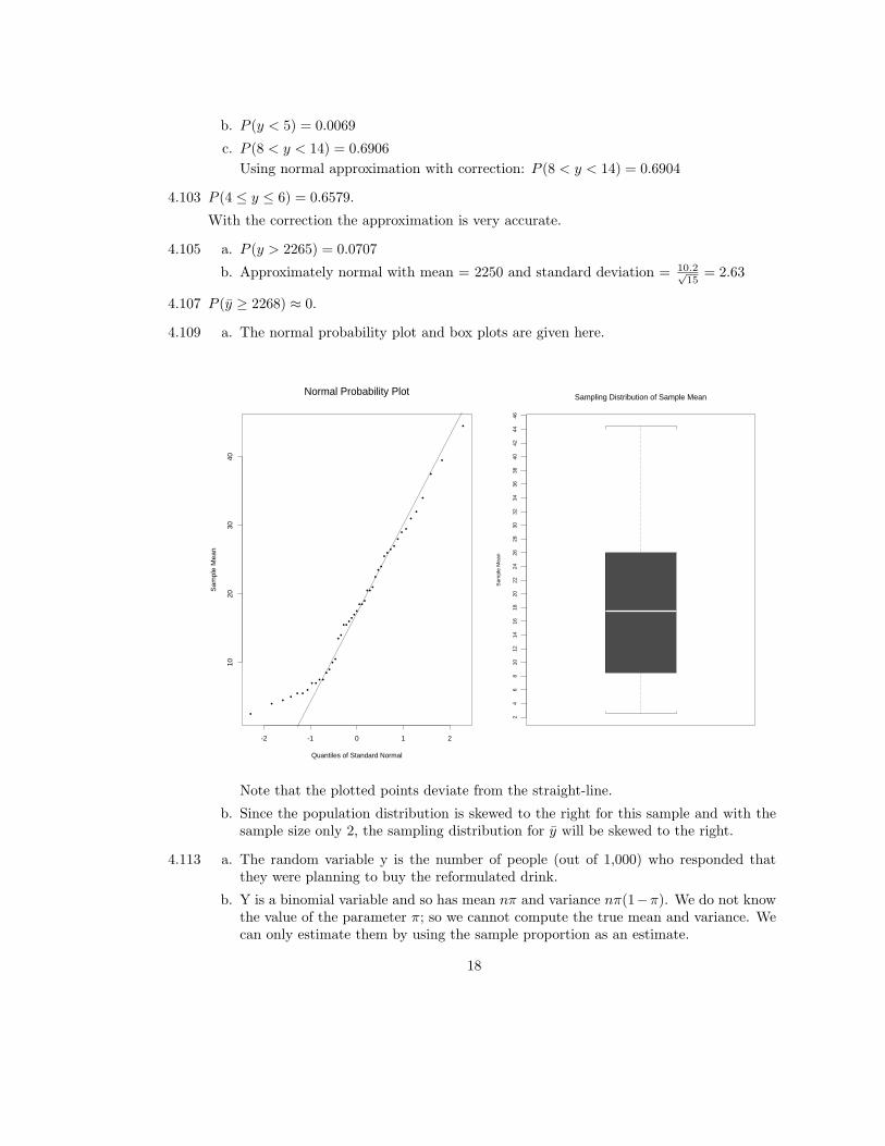
4.109 a. The normal probability plot and box plots are given here.
••
• ••
•
•
•
•
•• •
•
•
•
•
•
• ••
•
•
•
•
•
•
•
•
•
•
•
•
•
•
•
•
•
•
•
•
•
•
•
•
•
Normal Probability Plot
Quantiles of Standard Normal
Sam
ple
Mea
n
-2 -1 0 1 2
1020
3040
24
68
1012
1416
1820
2224
2628
3032
3436
3840
4244
46
Sampling Distribution of Sample Mean
Sam
ple
Mea
n
Note that the plotted points deviate from the straight-line.
b. Since the population distribution is skewed to the right for this sample and with thesample size only 2, the sampling distribution for y will be skewed to the right.
4.113 a. The random variable y is the number of people (out of 1,000) who responded thatthey were planning to buy the reformulated drink.
b. Y is a binomial variable and so has mean nπ and variance nπ(1−π). We do not knowthe value of the parameter π; so we cannot compute the true mean and variance. Wecan only estimate them by using the sample proportion as an estimate.
18

c. Using the sample estimate of π , we can compute P (y ≤ 250) by the normal approxi-mation if nπ and n(1− π) are both greater than 5.
4.115 n = 400 π = 0.2
a. P (y ≤ 25) ≈ 0.
b. The ad is not successful. With π = .20, we expect 80 positive responses out of 400 butwe observed only 25. The probability of getting so few positive responses is virtually0 if π = .20. We therefore conclude that π is much less than 0.20.
4.117 The sampling distribution of the sample mean consists of the following values for y andtheir frequency of occurrence.
y P (y) y P (y) y P (y) y P (y) y P (y)
7.25 1/70 17.00 1/70 21.50 2/70 26.00 1/70 35.75 1/7010.50 1/70 17.25 1/70 21.75 1/70 26.25 1/7011.25 1/70 17.50 1/70 22.25 2/70 26.50 1/7011.50 1/70 18.00 2/70 22.50 2/70 26.75 1/7012.00 1/70 18.25 1/70 23.25 2/70 27.50 2/7012.25 1/70 18.75 2/70 23.50 1/70 28.25 1/7013.00 2/70 19.00 1/70 23.75 1/70 29.00 2/7014.00 2/70 19.25 1/70 24.00 1/70 30.00 2/7014.75 1/70 19.50 1/70 24.25 2/70 30.75 1/7015.50 2/70 19.75 2/70 24.75 1/70 31.00 1/7016.25 1/70 20.50 2/70 25.00 2/70 31.50 1/7016.50 1/70 20.75 2/70 25.50 1/70 31.75 1/7016.75 1/70 21.25 1/70 25.75 1/70 32.50 1/70
4.119 The sampling distribution of the sample median consists of the following values for themedian (M) and their frequency of occurrence.
M P(M)
7.5 5/709.0 4/7010.5 8/7015.5 3/7017.0 6/7017.5 2/7018.5 9/7019.0 4/7020.5 6/7022.5 1/7024.0 2/7025.5 3/7027.0 8/7032.0 4/7034.0 5/70
4.120 a. The normal probability plot is given here.
19

• • • • •
• • • •
••••••••
•••
••••••••
•••••••••••••
••••••
•
••
•••
••••••••
• • • •
• • • • •
Normal Probability Plot for the Sample Median
Quantiles of Standard Normal
Sam
ple
Mea
n
-2 -1 0 1 2
1015
2025
3035
Note that the plotted points deviate considerably from the straight-line. Thus, thesampling distribution is not approximated very well by a normal distribution. If thesample size was much larger than 4 the approximation would be greatly improved.
b. The population median equals 12+252 = 18.5 whereas the mean of the 70 values of the
sample median is 19.536. The values differ by a significant amount due to the factthat the sample size was only 4.
4.121 a.,b. The mean and standard deviation of the sampling distribution of y are given whenthe population distribution has values µ = 100, σ = 15:
Sample Size Mean Standard Deviation
5 100 6.70820 100 3.35480 100 1.677
c. As the sample size increases, the sampling distribution of y concentrates about thetrue value of µ. For n = 5 and 20, the values of y could be a considerable distancefrom 100.
4.123 n = 36, µ = 40, σ = 12
a. The sampling distribution of y is approximately normal with a mean of 40 and astandard deviation of 2
b. P (y > 36) = 0.9772
20

c. P (y < 30) = .000000287
d. P (z > 1.645) = 43.29
4.125 a. Mean = 10, Standard Deviation = 2
b. Mean = 10, Standard Deviation = 1
c. Mean = 10, Standard Deviation = 4
d. Mean = 10, Standard Deviation = 2
Chapter 5: Inferences about Population Central Values
5.1 a. All registered voters in the state.
b. Simple random sample from a list of registered voters.
5.3 We might think that the actual average lifetime is less than the proposed 1500 hours.
a. The population is the lifetime of all fuses produced by the manufacturer during aselected period of time.
b. Testing a hypothesis.
5.5 a. (12.22, 12.38)
b. We are 95% confident that the average weight of a box of corn flakes is between 12.22and 12.38 oz.
5.7 a. 36
b. 7
c. 7
5.9 a. (−.92, 11.32)
b. Since the sample size is small, the condition that the distribution of profit marginsneeds to be normal is crucial. Similarly, with n=10, replacing σ with s is questionable.Section 5.7 will provide more details about this type of situation.
5.11 (3.02, 3.38)
5.13 (824.7, 875.3)
5.15 (412.9, 447.1)
5.17 (0.164, 0.196)
We are 95% confident that the mean protein content for the population is between 0.164and 0.196.
21
5.19 a. n decreases
b. n increases
c. n increases
5.21 125
5.23 a. σ = 1125
5.25 a. n = 94
b. The sample size is somewhat larger.
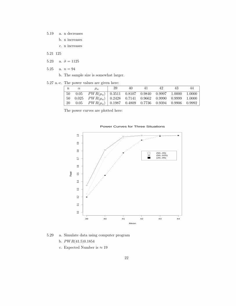
5.27 a.-c. The power values are given here:
n α µa 39 40 41 42 43 44
50 0.05 PWR(µa) 0.3511 0.8107 0.9840 0.9997 1.0000 1.000050 0.025 PWR(µa) 0.2428 0.7141 0.9662 0.9990 0.9999 1.000020 0.05 PWR(µa) 0.1987 0.4809 0.7736 0.9394 0.9906 0.9992
The power curves are plotted here:
Power Curves for Three Situations
Mean
Powe
r
39 40 41 42 43 44
0.00.1
0.20.3
0.40.5
0.60.7
0.80.9
1.0
(50,.05)(50,.025)(20,.05)
5.29 a. Simulate data using computer program
b. PWR(41.5)0.1854
c. Expected Number is ≈ 19
22
d. For µ = 38, PWR(38) = 0.2595
Expected Number is ≈ 26
For µ = 43, PWR(43) = 0.4424
Expected Number is ≈ 44
5.31 n =32
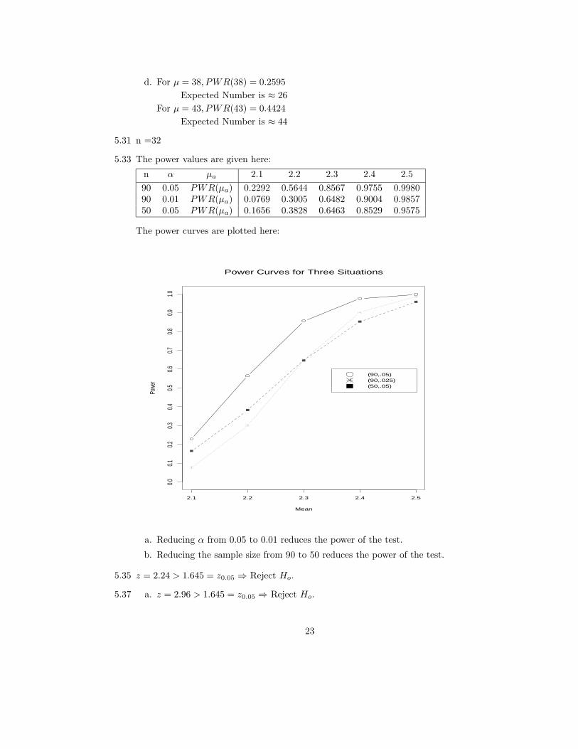
5.33 The power values are given here:
n α µa 2.1 2.2 2.3 2.4 2.5
90 0.05 PWR(µa) 0.2292 0.5644 0.8567 0.9755 0.998090 0.01 PWR(µa) 0.0769 0.3005 0.6482 0.9004 0.985750 0.05 PWR(µa) 0.1656 0.3828 0.6463 0.8529 0.9575
The power curves are plotted here:
Power Curves for Three Situations
Mean
Powe
r
2.1 2.2 2.3 2.4 2.5
0.00.1
0.20.3
0.40.5
0.60.7
0.80.9
1.0
(90,.05)(90,.025)(50,.05)
a. Reducing α from 0.05 to 0.01 reduces the power of the test.
b. Reducing the sample size from 90 to 50 reduces the power of the test.
5.35 z = 2.24 > 1.645 = z0.05 ⇒ Reject Ho.
5.37 a. z = 2.96 > 1.645 = z0.05 ⇒ Reject Ho.
23

b. Probability of Type I error is 0.05.
Probability of Type II error is 0
5.39 Ho : µ ≤ 0.3 vs Ha : µ > 0.3
a. z = 7.75 > 1.645 = z0.05 ⇒ Reject Ho.
b. Since we are interested in testing µ > 0.3, a two-tailed test would not be appropriate.
5.41 p-value = 0.0359 > 0.025 = α⇒No
5.43 Yes
5.45 p-value = 0.8078 > 0.05 = α⇒No
5.47 Ho : µ = 1.6 versus Ha : µ 6= 1.6,
p− value < 0.0001 < 0.05 = α⇒Yes
5.49 a. Reject Ho if t ≤ −1.761
b. Reject Ho if |t| ≥ 2.074
c. Reject Ho if t ≥ 2.015
5.51 Reject Ho if t ≥ t.05,17 = 1.740
t = 1.64⇒ Fail to reject Ho
5.53 Ho : µ ≤ 80 versus Ha : µ > 80, n = 20, Reject Ho if t ≥ 1.729.
t = 0.84⇒Fail to reject Ho
The level of significance is given by p-value = P (t ≥ 0.84) ≈ 0.20 > 0.05 = α.
5.55 a. (27600, 35340) is a 99% C.I. on the mean miles driven.
b. Ho : µ ≥ 35 versus Ha : µ < 35 Reject Ho if t ≤ −2.624.
t = −2.71⇒Reject Ho
0.005 < p− value < 0.01.
5.57 a. (4.57, 5.33) is a 95% C.I. on the mean dissolved oxygen level.
b. There is inconclusive evidence that the mean is less than 5
c. Ho : µ ≥ 5 versus Ha : µ < 5, t = −0.31 ⇒ 0.25 < p − value < 0.40 ⇒ Fail to rejectHo
5.59 a. Untreated: (40.3, 46.9)
Treated: (33.3, 38.9)
b. The average heights of the treated and untreated shrups are significantly different.
24

5.60 Before: (20.76, 25.68)
After: (22.87, 27.79)
There is not strong evidence of an increase
5.61 a. Ho : µAfter − µBefore ≤ 0 versus Ha : µAfter − µBefore > 0 which implies
Ho : µAfter ≤ µBefore versus Ha : µAfter > µBeforet = 0.88⇒ p− value = 0.2009 > 0.05
There is not evidence that the mean change in mpg is greater than 0, i.e., the meanmpg does not appear to be increased after installing the device.
b. (−2.26, 6.48)⇒Reject Ho : µ ≤ µo in favor of Ha : µ > µo if µo is less than the lower limit of the C.I.,we fail to reject Ho
5.62 a. Let µC = µAfter − µBefore. The probabilities of Type II error with d = |µa−0|7.54 are
given here:
µC 1.0 2.0 3.0 4.0 5.0 6.0 7.0 8.0 9.0
d 0.13 .27 .40 0.53 0.66 .80 .93 1.06 1.19
β(µa) 0.89 0.81 0.68 0.54 0.39 0.25 0.14 0.07 0.03
b. The sample size should be increased.
5.63 a. L.05 = 5, U.05 = 16
b. L.05 = 6, U.05 = 15
The intervals are somewhat narrower.
5.65 Reject Ho if B ≥ 20
5.67 Reject Ho if B ≤ 20 or B ≥ 33
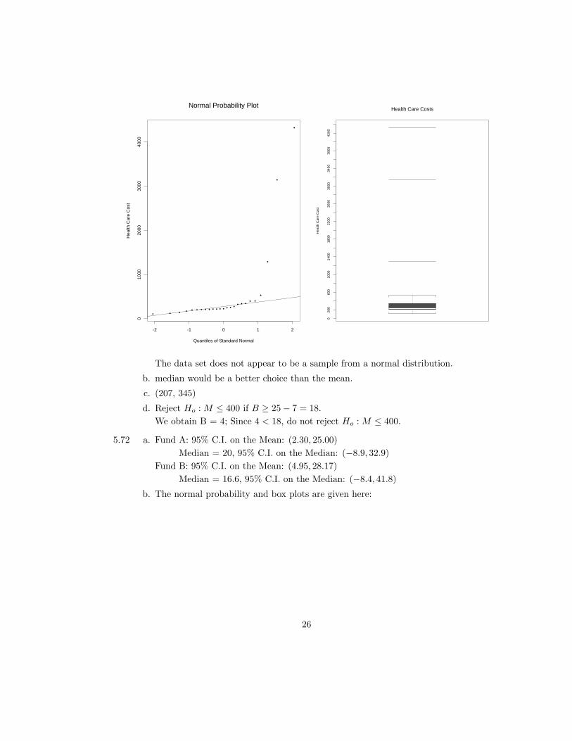
5.69 a. The normal probability plot is given here:
25
•
•
••••
•
•
•
•• ••
• •• • ••
•
•
•••
•
Normal Probability Plot
Quantiles of Standard Normal
Hea
lth C
are
Cos
t
-2 -1 0 1 2
010
0020
0030
0040
00
020
060
010
0014
0018
0022
0026
0030
0034
0038
0042
00
Health Care Costs
Hea
lth C
are
Cos
t
The data set does not appear to be a sample from a normal distribution.
b. median would be a better choice than the mean.
c. (207, 345)
d. Reject Ho : M ≤ 400 if B ≥ 25− 7 = 18.
We obtain B = 4; Since 4 < 18, do not reject Ho : M ≤ 400.
5.72 a. Fund A: 95% C.I. on the Mean: (2.30, 25.00)
Median = 20, 95% C.I. on the Median: (−8.9, 32.9)
Fund B: 95% C.I. on the Mean: (4.95, 28.17)
Median = 16.6, 95% C.I. on the Median: (−8.4, 41.8)
b. The normal probability and box plots are given here:
26

•
•
•
•
•
•
•
•
•
•
Normal Probability Plot
Quantiles of Standard Normal
Ret
urns
Fun
d A
-1 0 1
-10
010
2030
-10
-8-6
-4-2
02
46
810
1214
1618
2022
2426
2830
3234
Annual Rate of Return - Fund A
Ret
urns
Fun
d A
•
•
•
•
•
•
•
•
•
•
Normal Probability Plot
Quantiles of Standard Normal
Ret
urns
Fun
d B
-1 0 1
-10
010
2030
40
-10
-50
510
1520
2530
3540
Annual Rate of Return - Fund B
Ret
urns
Fun
d B
5.73 a. Using α = 0.05; Reject Ho : M ≤ 10 in favor of Ho : M > 10 if B ≥ 9
Fund A: B = 6⇒ Fail to reject Ho
Fund B: B = 6⇒ Fail to reject Ho
27
b. Using α = 0.05; Reject Ho if p-value ≤ 0.05.
Fund A: t = 0.73⇒ p− value = 0.24⇒ Fail to reject Ho
Fund B: t = 1.28⇒ p− value = 0.12⇒ Fail to reject Ho
5.77 a. Ha : µ 6= 220
b. Reject Ho if |z| ≥ 1.96. Since z − 2.18⇒ Reject Ho
c. p− value = 0.0292
d. 95% C.I.: (197.22, 218.78)
5.79 a. y = 1.466
b. 95% C.I.: (1.26, 1.67)
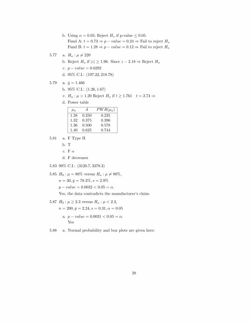
c. Ha : µ > 1.20 Reject Ho if t ≥ 1.761 t = 2.74⇒d. Power table
µa d PWR(µa)
1.28 0.250 0.2351.32 0.375 0.3961.36 0.500 0.5781.40 0.625 0.744
5.81 a. F Type II
b. T
c. F α
d. F decreases
5.83 99% C.I.: (3120.7, 3379.3)
5.85 H0 : µ = 80% versus Ha : µ 6= 80%,
n = 30, y = 78.3%, s = 2.9%
p− value = 0.0032 < 0.05 = α.
Yes, the data contradicts the manufacturer’s claim.
5.87 H0 : µ ≥ 2.3 versus Ha : µ < 2.3,
n = 200, y = 2.24, s = 0.31, α = 0.05
a. p− value = 0.0031 < 0.05 = α.
Yes
5.88 a. Normal probability and box plots are given here:
28

•
•
•
•
•
• •
•
•
•
•
•
•
• •
•
•
•
• •
•
•
•
•
Normal Probability Plot
Quantiles of Standard Normal
Dis
solu
tion
Rat
e
-2 -1 0 1 2
19.5
20.0
20.5
19.2
19.3
19.4
19.5
19.6
19.7
19.8
19.9
20.0
20.1
20.2
20.3
20.4
20.5
20.6
20.7
20.8
Dissolution Rates from Assays
Dis
solu
tion
Rat
e
b. 99% C.I.: (19.58, 20.08)
c. H0 : µ ≥ 20 versus Ha : µ < 20,
n = 24, y = 19.83, s = 0.43, α = 0.01
p− value = 0.0324 > 0.01 = α.
No
d. From Table 3 in Appendix with d = |19.6−20|.43 = .93, df = 23, α = 0.01, we obtain
β(19.6) = .025
5.91 a. y = 74.2 95% C.I.: (49.72, 98.68)
b. H0 : µ ≤ 50 versus Ha : µ > 50,
n = 15, α = 0.05
p− value = 0.0262 < 0.05 = α.
Yes
5.93 a. 95% C.I.: (8.73, 9.13)
c. H0 : µ = 9 versus Ha : µ 6= 9,
n = 12, α = 0.05
p− value = 2P (t ≥ 0.77) = 0.4562 > 0.05 = α.
No
5.95 a. T
29

b. F
c. T
d. T
e. F
f. T
5.97 a. Ho : µ ≥ 10 versus Ha : µ < 10
Reject Ho is z ≤ −1.645
z = −2
Reject Ho.
b. Yes; No; Yes; No
5.99 Ho : µ ≥ 8.2;Ha : µ < 8.2
z = −2.36
The level of significance is given by p-value = P (z < −2.36) = 0.0091 < 0.05 = α.
Thus, reject Ho
5.101 a. y = 30.514, s = 12.358, n = 35
95% C.I.: (26.27, 34.76)
We are 95% confident that this interval captures the population mean exercise capacity.
b. 99% C.I.: (24.81, 36.21)
The 99% C.I. is somewhat wider that the 95% C.I.
5.102 n = (12.36)2(1.96)2
(1)2 = 586.9⇒ n = 587
5.105 n = 30, y = 98.4, s = 0.15
90% C.I. on µ : (98.35, 98.45)
5.109 n = 50, y = 75, s = 15
95% C.I. on µ : (70.7, 79.3)
5.111 n = 40, y = 35, s = 6.3
95% C.I. on µ : (33.0, 37.0)
5.113 n = 312
5.115 n = 171
30
Chapter 6: Comparing Two Population Central Values
6.1 a. Reject Ho if |t| ≥ 2.064
b. Reject Ho if t ≥ 2.624
c. Reject Ho if t ≤ −1.860
6.5 a. Ho : µA = µB versus Ha : µA 6= µB ; p− value = 0.065⇒b. The separate variance t’-test was used.
d. The 95% C.I. estimate for the difference in means is (-0.013, 0.378) ppm. The observeddifference (0.183 ppm) is not significant.
6.7 We want to test Ho : µNo = µSub versus Ha : µNo 6= µSub; p− value = 0.0049⇒Reject Ho
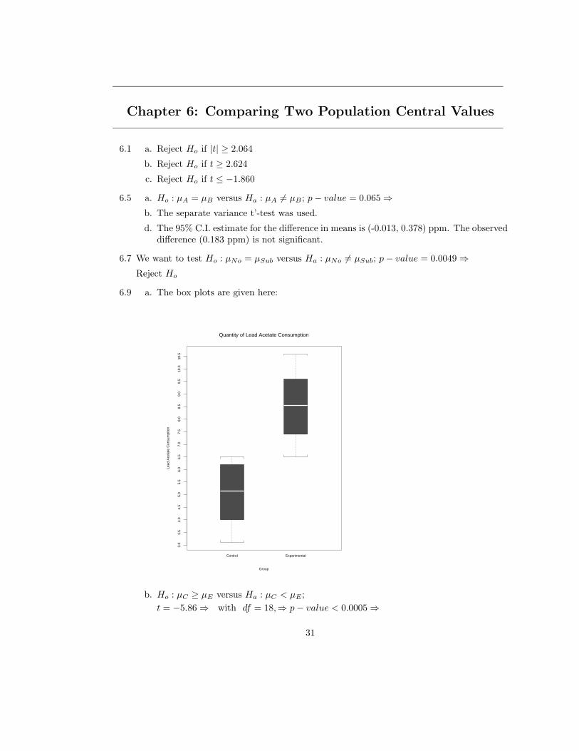
6.9 a. The box plots are given here:
3.0
3.5
4.0
4.5
5.0
5.5
6.0
6.5
7.0
7.5
8.0
8.5
9.0
9.5
10.0
10.5
Control Experimental
Quantity of Lead Acetate Consumption
Group
Lead
Ace
tate
Con
sum
ptio
n
b. Ho : µC ≥ µE versus Ha : µC < µE ;
t = −5.86⇒ with df = 18,⇒ p− value < 0.0005⇒
31
Reject Ho
A 95% C.I. on the difference in the mean quantity of lead acetate consumed is (-4.76,-2.24)
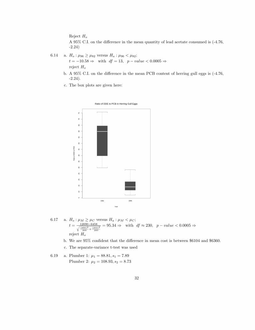
6.14 a. Ho : µ96 ≥ µ82 versus Ha : µ96 < µ82;
t = −10.58⇒ with df = 13, p− value < 0.0005⇒reject Ho
b. A 95% C.I. on the difference in the mean PCB content of herring gull eggs is (-4.76,-2.24).
c. The box plots are given here:
510
1520
2530
3540
4550
5560
6570
75
1982 1996
Ratio of DDE to PCB in Herring Gull Eggs
Year
Rat
io o
f DD
E to
PC
B
6.17 a. Ho : µM ≥ µC versus Ha : µM < µC ;
t = 12690−6458√(890)2
200 +(250)2
200
= 95.34⇒ with df ≈ 230, p− value < 0.0005⇒
reject Ho
b. We are 95% confident that the difference in mean cost is between $6104 and $6360.
c. The separate-variance t-test was used
6.19 a. Plumber 1: µ1 = 88.81, s1 = 7.89
Plumber 2: µ2 = 108.93, s2 = 8.73
32

b. The box plots are given here:
7075
8085
9095
100
105
110
115
120
125
Dispatched Sequential
Comparison of Efficiency of Dispatch Systems
System
Tot
al D
aily
Mile
age
A t-test appears to be appropriate.
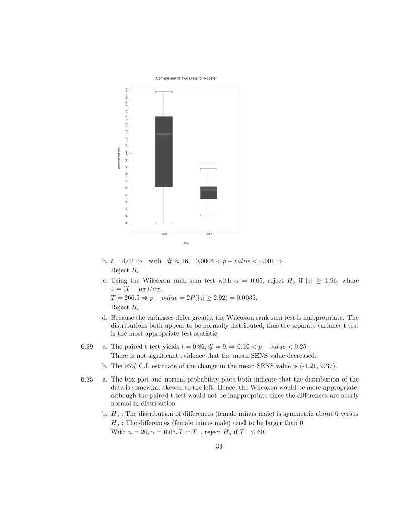
6.21 a. Box plots are given here:
33
5055
6065
7075
8085
9095
100
105
110
115
120
125
130
135
140
145
Diet I Diet II
Comparison of Two Diets for Rooster
Diet
Wei
ghts
(m
illig
ram
s)
b. t = 4.07⇒ with df ≈ 16, 0.0005 < p− value < 0.001⇒Reject Ho
c. Using the Wilcoxon rank sum test with α = 0.05, reject Ho if |z| ≥ 1.96, wherez = (T − µT )/σT .
T = 266.5⇒ p− value = 2P (|z| ≥ 2.92) = 0.0035.
Reject Ho
d. Because the variances differ greatly, the Wilcoxon rank sum test is inappropriate. Thedistributions both appear to be normally distributed, thus the separate variance t testis the most appropriate test statistic.
6.29 a. The paired t-test yields t = 0.86, df = 9,⇒ 0.10 < p− value < 0.25
There is not significant evidence that the mean SENS value decreased.
b. The 95% C.I. estimate of the change in the mean SENS value is (-4.21, 9.37).
6.35 a. The box plot and normal probability plots both indicate that the distribution of thedata is somewhat skewed to the left. Hence, the Wilcoxon would be more appropriate,although the paired t-test would not be inappropriate since the differences are nearlynormal in distribution.
b. Ho : The distribution of differences (female minus male) is symmetric about 0 versus
Ha : The differences (female minus male) tend to be larger than 0
With n = 20, α = 0.05, T = T−, reject Ho if T− ≤ 60.
34

From the data we obtain T− = 18 < 60, thus reject Ho and conclude that repair costsare generally higher for female customers.
6.37 a. Population of interest is the collection of all steel beams made from both the new andold alloy.
b. 99% C.I. on Old Alloy Mean Load Capacity: (22.12, 24.62)
99% C.I. on New Alloy Mean Load Capacity: (26.27, 31.43)
99% C.I. on µOld − µNew: (-8.14, -2.82)
c. Ho : µOld ≥ µNew versus Ha : µOld < µNew;
t = 6.21⇒ with df ≈ 13, p− value < 0.0005⇒reject Ho
d. Box plots are given here:
24
68
1012
1416
1820
2224
26
Old Alloy New Alloy
Comparison of Load Capacity of Two Alloys
Type of Alloy
Load
Cap
acity
(to
ns)
The separate-variance t-test was used since s2New is 4.2 times larger than s2
Old, but thedistributions both appear normally distributed.
e. The company should not switch alloys because the C.I. on µOld−µNew indicates thatthe difference may be as small as -2.82 units.
6.39 a. Ho : µNarrow = µWide versus Ha : µNarrow 6= µWide;
t = 3.17⇒ with df ≈ 17, 0.005 < p− value < 0.01⇒reject Ho
35

b. A 95% C.I. on µWide − µNarrow is (2.73, 13.60)
6.42 a. Ho : µWithin = µOut versus Ha : µWithin 6= µOut;
t = 3092−2450√(1191)2
14 +(2229)2
12
= 0.89⇒ with df ≈ 16, p− value ≈ 0.384⇒
Fail to reject Ho
b. A 95% C.I. on µWithin − µOut is (-879, 2164)
d. Box plots are given here:
500
1000
1500
2000
2500
3000
3500
4000
4500
5000
5500
6000
6500
7000
7500
Within Outside
Evaluation of Effects of Oil Spill
Location
Pop
ulat
ion
Abu
ndan
ce (
coun
ts p
er s
q. m
eter
)
6.43 a. Ho : µWithin = µOut versus Ha : µWithin 6= µOut;
Since both n1, n2 are greater than 10, the normal approximation can be used.
T = 122⇒ p− value = 0.0394⇒reject Ho
b. The Wilcoxon rank sum test requires independently selected random samples fromtwo populations which have the same shape but may be shifted from one another.
c. The two population distributions may have different variances but the Wilcoxon ranksum test is very robust to departures from the required conditions.
d. The separate variance test failed to reject Ho with a p-value of 0.384. The Wilcoxontest rejected Ho with a p-value of 0.0394. The difference in the two procedures isprobably due to the skewness observed in the Outside data set. This can result ininflated p-values for the t test which relies on a normal distribution when the samplesizes are small.
36

6.44 a. Box plot is given here:
500
1000
1500
2000
2500
3000
3500
4000
4500
5000
5500
6000
6500
7000
7500
Within-40m Within-100m Outside-40m Outside-100m
Evaluation of Effects of Oil Spill
Location-Depth
Pop
ulat
ion
Abu
ndan
ce (
coun
ts p
er s
q. m
eter
)
b. 40M: Ho : µWithin = µOut versus Ha : µWithin 6= µOut;
t0.08⇒ with df ≈ 6, p− value ≈ 0.94⇒fail to reject Ho
100M: Ho : µWithin = µOut versus Ha : µWithin 6= µOut;
t = 2.50⇒ with df ≈ 7, p− value ≈ 0.041⇒reject Ho
6.49 a. Ho : µD1= µD2
versus Ha : µD16= µD2
;
Since s1 = 13.49 and s2 = 18.49, there is not strong evidence that the populationvariances are unequal, hence use a pooled t-test:
t = −1.35 with df = 18, p− value ≈ 0.19.⇒Fail to reject Ho
b. p− value ≈ 0.19
c. 95% C.I. on µD1− µD2
: (-25.0, 5.4) minutes
6.51 a. Ho : µHigh = µCon versus Ha : µHigh 6= µCon;
Separate variance t-test: t = 4.12 with df ≈ 34, p− value = 0.0002.⇒Reject Ho
b. 95% C.I. on µHigh − µCon: (19.5, 57.6)
37

6.52 a. Ho : µLow = µCon versus Ha : µLow 6= µCon;
Separate variance t-test: t = −2.09 with df ≈ 35, p− value = 0.044.⇒Reject Ho
b. 95% C.I. on µLow − µCon: (-51.3, -0.8)
6.53 a. Ho : µLow = µHigh versus Ha : µLow 6= µHigh;
Separate variance t-test: t = −5.73 with df ≈ 29, p− value < 0.0005.⇒Reject Ho
b. 95% C.I. on µLow − µHigh: (-87.6, -41.5),
6.54 a. Let Ai be the event that a Type I error was made on the ith test, i = 1, 2, 3.
P(at least one Type I error in 3 tests) = P (A1 ∪A2 ∪A3)
= P (A1)+P (A2)+P (A3)−P (A1∩A2)−P (A1∩A3)−P (A2∩A3)+P (A1∩A2∩A3)
≤ P (A1) + P (A2) + P (A3) = 0.05 + 0.05 + 0.05 = 3(0.05) = 0.15
b. Set the value of α at 0.053 for each of the 3 tests.
Then P(at least one Type I error in 3 tests) ≤ 3( 0.053 ) = 0.05.
Thus, we know that the chance of at least one Type I error in the 3 tests is at most0.05.
6.59 a. Ho : µD ≤ µRN versus Ha : µD > µRN ;
Separate variance t-test: t = 9.04 with df ≈ 76, p− value < 0.0001⇒Reject Ho and conclude there is significant evidence that the mean score of the Degreednurses is higher than the mean scores of the RN nurses.
b. p− value < 0.0001
c. 95% C.I. on µD − µRN : (35.3, 55.2) points
6.63 a. Ho : µF ≥ µM versus Ha : µF < µM ;
b. 95% C.I. on µF − µM : (-142.30, -69.1) thousands of dollars
c. t = −5.85 with df = 38
p− value < 0.0001⇒Reject Ho
6.67 a. Ho : µStandard ≥ µNew versus Ha : µStandard < µNewSince s1 ≈ s2, use pooled t-test: t = −1.94 with df = 54, p− value = 0.029⇒Reject Ho
b. 95% C.I. on µNew − µStandard: (0.2, 10.2)
6.69 a. Ho : µLast ≥ µCurrent versus Ha : µLast < µCurrent
b. t = −35.3,With df = 198⇒ p− value ≈ 0
Reject Ho
6.71 Ho : µFor ≤ µUSA versus Ha : µFor > µUSA
Since s1 ≈ s2, use separate-variance t-test:t1.67,With df = 26⇒0.05 < p− value < 0.10
Fail to reject Ho
38
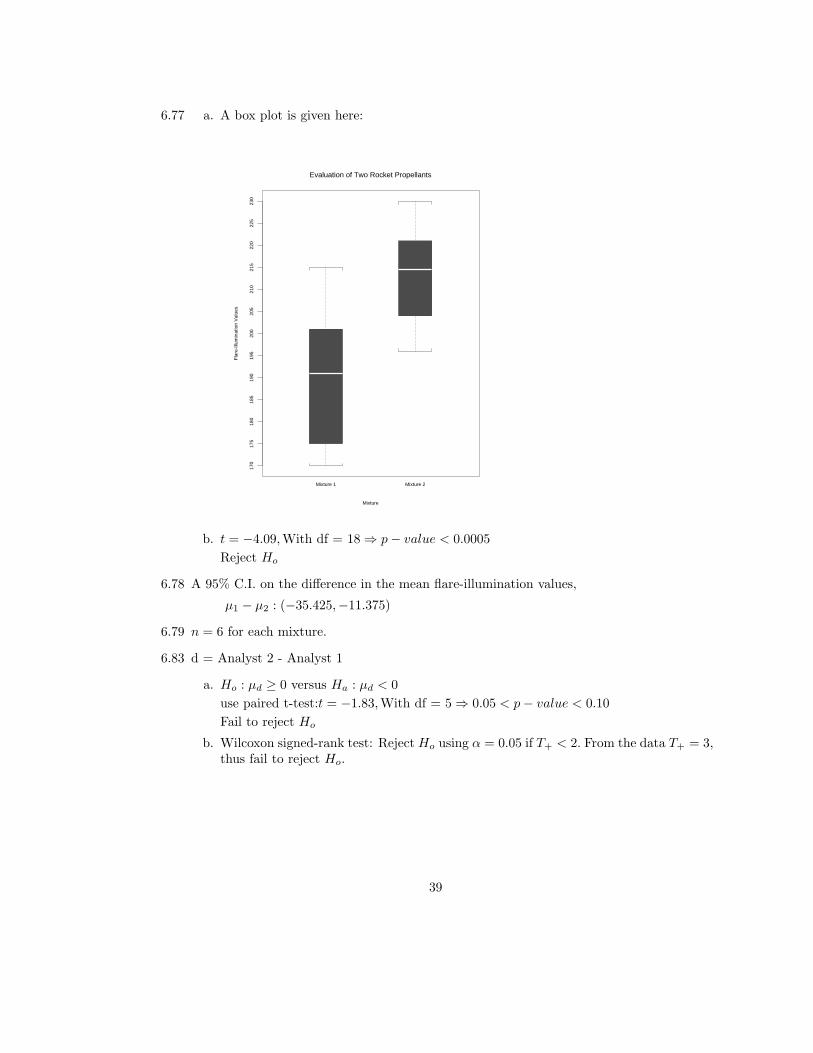
6.77 a. A box plot is given here:
170
175
180
185
190
195
200
205
210
215
220
225
230
Mixture 1 Mixture 2
Evaluation of Two Rocket Propellants
Mixture
Fla
re-I
llum
inat
ion
Val
ues
b. t = −4.09,With df = 18⇒ p− value < 0.0005
Reject Ho
6.78 A 95% C.I. on the difference in the mean flare-illumination values,
µ1 − µ2 : (−35.425,−11.375)
6.79 n = 6 for each mixture.
6.83 d = Analyst 2 - Analyst 1
a. Ho : µd ≥ 0 versus Ha : µd < 0
use paired t-test:t = −1.83,With df = 5⇒ 0.05 < p− value < 0.10
Fail to reject Ho
b. Wilcoxon signed-rank test: Reject Ho using α = 0.05 if T+ < 2. From the data T+ = 3,thus fail to reject Ho.
39

Chapter 7: Inferences about Population Variances
7.1 a. 0.01
b. 0.90
c. 0.01
d. 0.98
7.3 a. 106.632
57.1462
Rounded to 2 decimal places, the above approximations are exactly the values givenin Table 7 for the Chi-square distribution.
b. 324.999
232.787
7.5 a. Let y be the quantity in a randomly selected jar:
Proportion = 2.28%
b. The plot indicates that the distribution is approximately normal because the datavalues are reasonably close to the straight-line.
c. 95% C.I. on σ : (0.113, 0.168)
d. Ho : σ ≤ 0.15 versus Ha : σ > 0.15
Reject Ho if (n−1)(s)2
(.15)2 ≥ 66.34
Fail to reject Ho
e. 0.10 < p− value < 0.90
(Using a computer program, p-value = 0.8262).
7.7 a. n = 26, y = 3.999, s = 0.0159
b. Ho : σ ≤ 0.011 versus Ha : σ > 0.011
Reject Ho if (n−1)(s)2
(.011)2 ≥ 37.65
Reject Ho
7.8 90% C.I. on σ : (0.01297, 0.02080)
7.9 The box plot and normal probability plot is given here:
40

•
•
•
•
•
•
•
•
•
•
•
•
•
•
•
•
•
•
•
•
•
•
•
•
•
•
Normal Probability Plot
Quantiles of Standard Normal
Dia
met
er
-2 -1 0 1 2
3.96
3.98
4.00
4.02
4.04
3.95
03.
960
3.97
03.
980
3.99
04.
000
4.01
04.
020
4.03
04.
040
Evaluation of Deviation from a 4.000 mm Specification
Assemply Part
Dia
met
er (
mm
)
7.13 a. α = .05, df1 = 7, df2 = 12,⇒ F0.05 = 2.91
b. α = .05, df1 = 3, df2 = 10,⇒ F0.05 = 3.71
c. α = .05, df1 = 10, df2 = 20,⇒ F0.05 = 2.35
d. α = .01, df1 = 8, df2 = 15,⇒ F0.01 = 4.00
e. α = .01, df1 = 12, df2 = 25,⇒ F0.01 = 2.99
7.15 Ho : σ21 = σ2
2 versus Ha : σ21 6= σ2
2
With α = 0.10, reject Ho ifs21s22≤ 1
3.68 = 0.272 ors21s22≥ 3.29
s21/s
22 = 0.583⇒ 0.272 < 0.583 < 3.29⇒
Fail to reject Ho
7.17 a. 95% C.I. on σOld : (0.196, 0.281)
95% C.I. on σNew : (0.137, 0.197)
b. Ho : σ2Old ≤ σ2
New versus Ha : σ2Old > σ2
New
With α = 0.05, reject Ho ifs2Olds2New
≥ 1.53
s2Old/s
2New = 2.033 > 1.53⇒
Reject Ho
41

7.21 b. With α = 0.01, reject Ho if Fmax > 9.9
Fmax = 80.226.89 = 11.64 > 9.9⇒
Reject Ho at level α = 0.01
The Levine test yields L = 4.545 with df1 = (3− 1) = 2, df2 = (27− 3) = 24
With α = 0.01, reject Ho if L > F.01,2,24 = 5.61
L = 4.545 < 5.61⇒ Fail to reject Ho at the 0.01 level.
Thus, the Levine and Hartley test yield contradictory conclusions.
c. When the population distributions are normally distributed, the Hartley test is morepowerful than the Levine test. Thus, in this situation, we would prefer the Hartleytest.
d. 95% C.I. on σ1 : (1.99, 5.65)
95% C.I. on σ2 : (1.77, 5.03)
95% C.I. on σ3 : (6.05, 17.16)
7.25 The data is summarized in the following table:
Method n Mean 95% C.I. on µ St.Dev. 95% C.I. on σ
L 10 5.90 (2.34, 9.46) 4.9766 (3.42, 9.09)L/R 7 7.29 (2.31, 12.26) 5.3763 (3.46,11.84)L/C 9 16.00 (9.57, 22.43) 8.3666 (5.65, 16.03)
C 9 17.67 (5.45, 29.88) 15.8902 (10.73, 30.44)
Test Ho : σL = σL/R = σL/C = σC versus Ha : σ′s are different
Reject Ho at level α = 0.05 if L ≥ F.05,3,31 = 2.91
From the data, L = 2.345 < 2.91⇒Fail to reject Ho
7.27 a. The box plots are given here:
42

3233
3435
3637
3839
4041
4243
4445
4647
4849
Brand I Brand II
Longevity of Two Brands of Tires
Brand of Tire
Mile
s to
Tire
Wea
rout
(10
00 m
iles)
b. The C.I.’s are given here:
Method n Mean 95% C.I. on µ St.Dev. 95% C.I. on σ
I 10 38.79 (37.39, 40.19) 1.9542 (1.34, 3.57)II 10 40.67 (36.68, 44.66) 5.5791 (3.84, 10.19)
c. A comparison of the population variances yields:
Ho : σ2I = σ2
II versus Ha : σ2I 6= σ2
II
With α = 0.01, reject Ho ifs2Is2II≤ 1
6.54 = 0.15 ors21s22≥ 6.54
s21/s
22 = (5.5791)2/(1.9542)2 = 8.15 > 6.54⇒
Reject Ho
Ho : µI = µII versus Ha : µI 6= µII
t = −1.01 with df=11 ⇒ p− value = 0.336
Fail to reject Ho
7.29 a. 25x90% = 22.5 and 25x110% = 27.5 implies the limits are 22.5 to 27.5
b. The box plot and normal probability plot are given here:
43

•
•
•
•
•
••
•
•
•
•
•
•
•
•
•
•
•
•
•
•
•
•
•
•
•
•
••
•
Normal Probability Plot
Quantiles of Standard Normal
Pot
ency
of T
able
t
-2 -1 0 1 2
2324
2526
27
23.0
23.5
24.0
24.5
25.0
25.5
26.0
26.5
27.0
Potency of Antihistamine Tablets
Tablets
Pot
ency
of T
able
t
c. σ = 5/4 = 1.25
Ho : σ = 1.25 versus Ha : σ 6= 1.25
With α = 0.05, reject Ho if (n−1)s2
(1.25)2 ≤ 16.05 or (n−1)s2
(1.25)2 ≥ 45.72
(30−1)(1.4691)2
(1.25)2 = 40.06⇒ 16.06 < 40.06 < 45.72
Fail to reject Ho
7.31 95% C.I. on σ2 : (3.15, 11.63)
The 95% C.I. fails to support the test findings of the consumer group.
7.33 Ho : µ1 = µ2 versus Ha : µ1 6= µ2
t = −7.09 with df=18 ⇒ p− value < 0.0005
Reject Ho
7.37 Summary statistics are given here: (C.I.’s are given for the median. C.I.’s for µ′s andσ′s are not appropriate because the distributions are nonnormal and the sample sizes arerelatively small)
Method n Mean Median 95% C.I. on Median St.Dev.
EXP 15 60.20 55.8 (51.4, 69.0) 10.8407MAR 15 53.63 52.7 (50.1, 55.8) 3.9808
The Wilcoxon test of differences in the two distributions yields
44

T = 280.5⇒ z = 1.99⇒ p− value = 0.0465 < 0.05⇒Box plots are given here:
5052
5456
5860
6264
6668
7072
7476
7880
8284
8688
Experimental Marketed
Comparison of Shelf Life of Two Drugs
Type of Drug
Dro
p in
Pot
ency
7.39 Box plots are given here:
45
1214
1618
2022
2426
2830
3234
3638
4042
4446
48
Preparation A Preparation B
Comparison of Weight-Reducing Agents
Type of Therapy
Leng
th o
f Tim
e on
The
rapy
(da
ys)
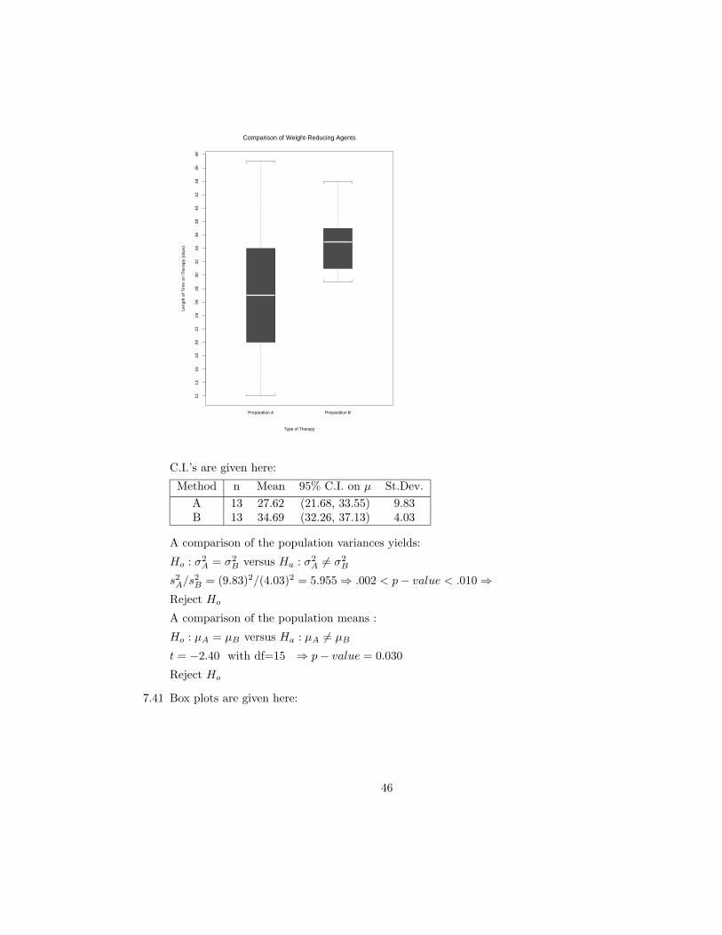
C.I.’s are given here:
Method n Mean 95% C.I. on µ St.Dev.
A 13 27.62 (21.68, 33.55) 9.83B 13 34.69 (32.26, 37.13) 4.03
A comparison of the population variances yields:
Ho : σ2A = σ2
B versus Ha : σ2A 6= σ2
B
s2A/s
2B = (9.83)2/(4.03)2 = 5.955⇒ .002 < p− value < .010⇒
Reject Ho
A comparison of the population means :
Ho : µA = µB versus Ha : µA 6= µB
t = −2.40 with df=15 ⇒ p− value = 0.030
Reject Ho
7.41 Box plots are given here:
46
1214
1618
2022
2426
2830
3234
3638
4042
4446
48
Preparation A Preparation B
Comparison of Weight-Reducing Agents
Type of Therapy
Leng
th o
f Tim
e on
The
rapy
(da
ys)
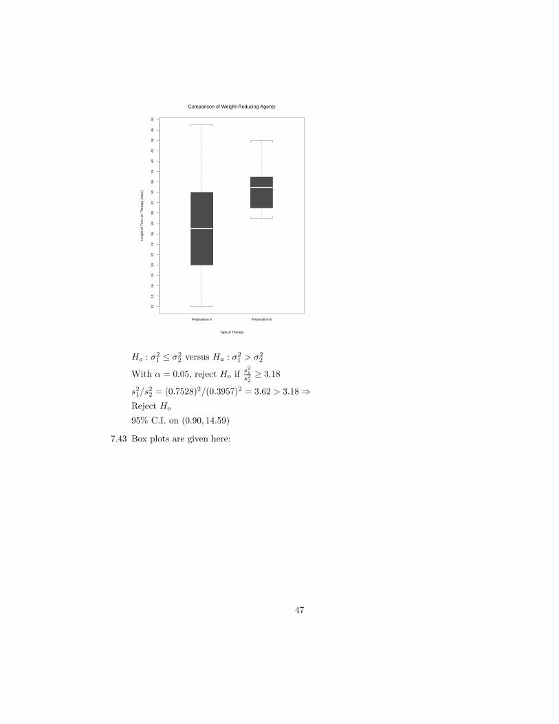
Ho : σ21 ≤ σ2
2 versus Ha : σ21 > σ2
2
With α = 0.05, reject Ho ifs21s22≥ 3.18
s21/s
22 = (0.7528)2/(0.3957)2 = 3.62 > 3.18⇒
Reject Ho
95% C.I. on (0.90, 14.59)
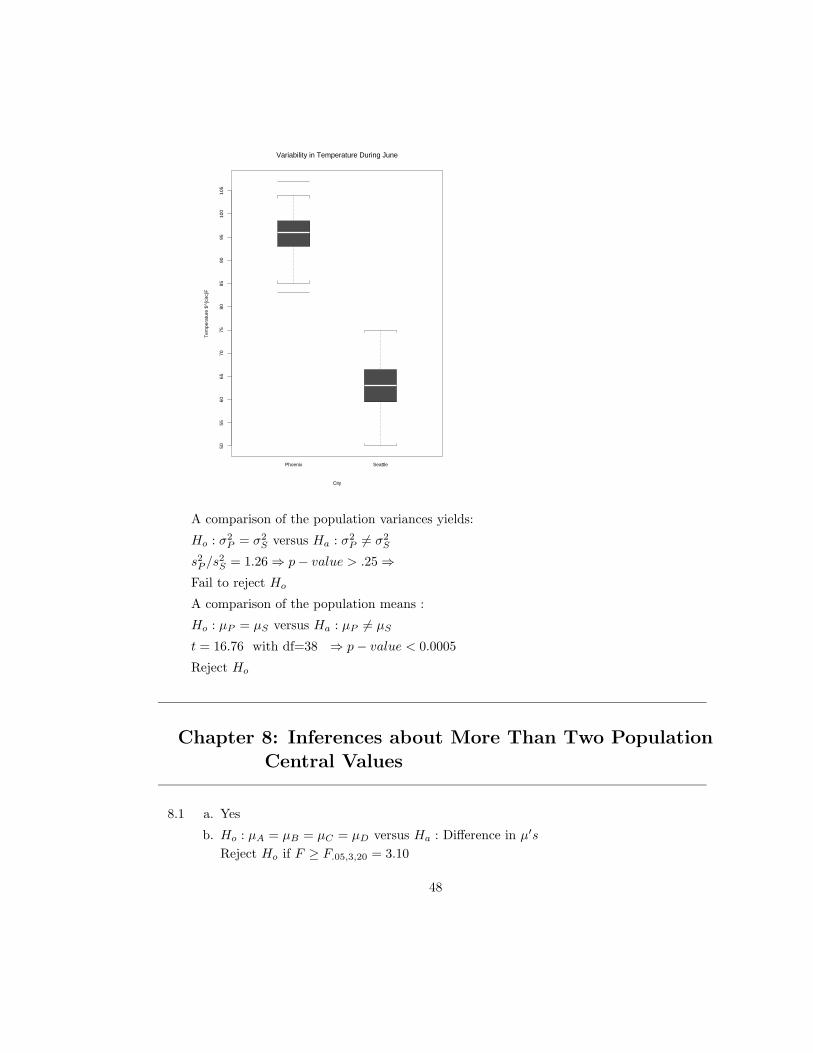
7.43 Box plots are given here:
47
5055
6065
7075
8085
9095
100
105
Phoenix Seattle
Variability in Temperature During June
City
Tem
pera
ture
$^{
circ
}F
A comparison of the population variances yields:
Ho : σ2P = σ2
S versus Ha : σ2P 6= σ2
S
s2P /s
2S = 1.26⇒ p− value > .25⇒
Fail to reject Ho
A comparison of the population means :
Ho : µP = µS versus Ha : µP 6= µS
t = 16.76 with df=38 ⇒ p− value < 0.0005
Reject Ho
Chapter 8: Inferences about More Than Two PopulationCentral Values
8.1 a. Yes
b. Ho : µA = µB = µC = µD versus Ha : Difference in µ′s
Reject Ho if F ≥ F.05,3,20 = 3.10
48

SSW = 0.8026
y.. = 0.0826⇒SSB = 0.5838⇒F = 4.85 > 3.10⇒Reject Ho
c. p− value = P (F3,20 ≥ 4.85)⇒ 0.01 < p− value < 0.025
8.3 Ho : µNE = µSE = µNW = µSW versus Ha : Difference in µ′s
Reject Ho if F ≥ F.05,3,20 = 3.10
SSW = 1.3367
y.. = 1.28925⇒SSB = 5.8312
F = 29.08 > 3.10⇒Reject Ho
8.5 a. Ho : µA = µB = µC versus Ha : Difference in µ′s
Reject Ho if F ≥ F.05,2,21 = 3.47
F = 9.98 > 10.09⇒Reject Ho
b. 95% C.I. on µA : (−0.592, 13.512)
95% C.I. on µB : (5.288, 19.392)
95% C.I. on µC : (20.298, 34.402)
c. Ho : µA = µB = µC versus Ha : Difference in µ′s
Reject Ho if F ≥ F.05,2,21 = 3.47
Using the transformed data: F = 10.00 > 3.47⇒Reject Ho The following C.I.’s are on the mean of the logarithm of the hours of reliefµi′ :
95% C.I. on µA′ : (1.305, 2.195)
95% C.I. on µB′ : (1.985, 2.875)
95% C.I. on µC′ : (2.655, 3.545)
d. The test of hypotheses using the raw and transformed yielded the same conclusion.
e. The inverse transformations involves exponentiating the endpoints of the C.I.:
95% C.I. on µA : (3.688, 8.980)
95% C.I. on µB : (7.279, 17.725)
95% C.I. on µC : (14.225, 34.640)
There is a considerable difference in the two sets of C.I.’s.
8.8 a. The Kruskal-Wallis yields H = 21.32 > 9.21 with df = 2⇒ p− value < 0.001. Thus,reject Ho
49
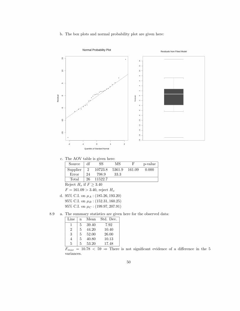
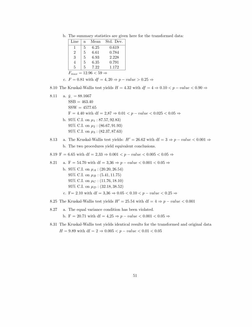
b. The box plots and normal probability plot are given here:
•
••
•
•
•
•
••
•
••
•
•
•
•
•
•
•
•
•
•
•
•
•
•
•
Normal Probability Plot
Quantiles of Standard Normal
Res
idua
l
-2 -1 0 1 2
-15
-10
-50
510
15
-18
-16
-14
-12
-10
-8-6
-4-2
02
46
810
1214
Residuals from Fitted Model
Res
idua
ls
c. The AOV table is given here:
Source df SS MS F p-value
Supplier 2 10723.8 5361.9 161.09 0.000Error 24 798.9 33.3Total 26 11522.7
Reject Ho if F ≥ 3.40
F = 161.09 > 3.40, reject Ho
d. 95% C.I. on µA : (185.26, 193.20)
95% C.I. on µB : (152.31, 160.25)
95% C.I. on µC : (199.97, 207.91)
8.9 a. The summary statistics are given here for the observed data:
Line n Mean Std. Dev.
1 5 39.40 7.922 5 44.20 10.403 5 52.00 26.004 5 40.80 10.135 5 53.20 17.48
Fmax = 10.78 < 59 ⇒ There is not significant evidence of a difference in the 5variances.
50
b. The summary statistics are given here for the transformed data:
Line n Mean Std. Dev.
1 5 6.25 0.6192 5 6.61 0.7843 5 6.93 2.2284 5 6.35 0.7915 5 7.22 1.172
Fmax = 12.96 < 59⇒c. F = 0.81 with df = 4, 20⇒ p− value > 0.25⇒
8.10 The Kruskal-Wallis test yields H = 4.32 with df = 4⇒ 0.10 < p− value < 0.90⇒
8.11 a. y.. = 88.1667
SSB = 463.40
SSW = 4577.65
F = 4.40 with df = 2,87 ⇒ 0.01 < p− value < 0.025 < 0.05⇒b. 95% C.I. on µ1 : 87.57, 92.83)
95% C.I. on µ2 : (86.67, 91.93)
95% C.I. on µ3 : (82.37, 87.63)
8.13 a. The Kruskal-Wallis test yields: H ′ = 26.62 with df = 3 ⇒ p− value < 0.001⇒b. The two procedures yield equivalent conclusions.
8.19 F = 6.65 with df = 2,33 ⇒ 0.001 < p− value < 0.005 < 0.05⇒
8.21 a. F = 54.70 with df = 3,36 ⇒ p− value < 0.001 < 0.05⇒b. 95% C.I. on µA : (20.20, 26.54)
95% C.I. on µB : (5.41, 11.75)
95% C.I. on µC : (11.76, 18.10)
95% C.I. on µD : (32.18, 38.52)
c. F= 2.10 with df = 3,36 ⇒ 0.05 < 0.10 < p− value < 0.25⇒
8.25 The Kruskal-Wallis test yields H ′ = 25.54 with df = 4 ⇒ p− value < 0.001
8.27 a. The equal variance condition has been violated.
b. F = 20.71 with df = 4,25 ⇒ p− value < 0.001 < 0.05⇒
8.31 The Kruskal-Wallis test yields identical results for the transformed and original data
H = 9.89 with df = 2 ⇒ 0.005 < p− value < 0.01 < 0.05
51

Chapter 9: Multiple Comparisons
9.1 a. Yes
b. No
9.3 a. l1 = 4µ1 − µ2 − µ3 − µ4 − µ5
b. l2 = 3µ2 − µ3 − µ4 − µ5
c. l3 = µ3 − 2µ4 + µ5
d. l4 = µ3 − µ5
9.5 Reject Ho if F = SSCMSError
> 4.11 (F0.05, df1 = 1, df2 = 36)
SSC = (l)2
∑i(a
2i /ni)
= 10(l)2
∑i a
2i
Using the transformed data, MSError = 0.2619
a. l1 = −8.51⇒ SSC1 = 60.35⇒ F = 230.43⇒Reject Ho
b. l2 = −5.51⇒ SSC2 = 50.60⇒ F = 193.20⇒Reject Ho
d. Yes
e. Yes
9.8 a. Fisher’s LSD: Pairs Not Significantly Different: (4,1), (2,3)
b. Tukey’s W: Pairs Not Significantly Different: (4,1), (4,2), (1,2), (2,3), (3,S)
c. SNK procedure: Pairs Not Significantly Different: (4,1), (2,3)
9.9 a. Tukey’s W
b. Fisher’s LSD
9.10 Using the computer output, the Dunnett procedure indicates that all four agents hadsignificantly larger average weight loss than the standard agent.
9.11 a. l1 = µA1+ µA2
+ µA3+ µA4
− 4µS
b. l2 = µA1− µA2
+ µA3− µA4
c. l3 = µA1+ µA2
− µA3− µA4
d. l4 = µA1+ µA3
− 2µS
9.12 Using Scheffe’s Method:
Si = 1.0066√∑
i a2i
Declare contrast li significantly different from 0 if |li| > Si
The tests are summarized as follows:
52
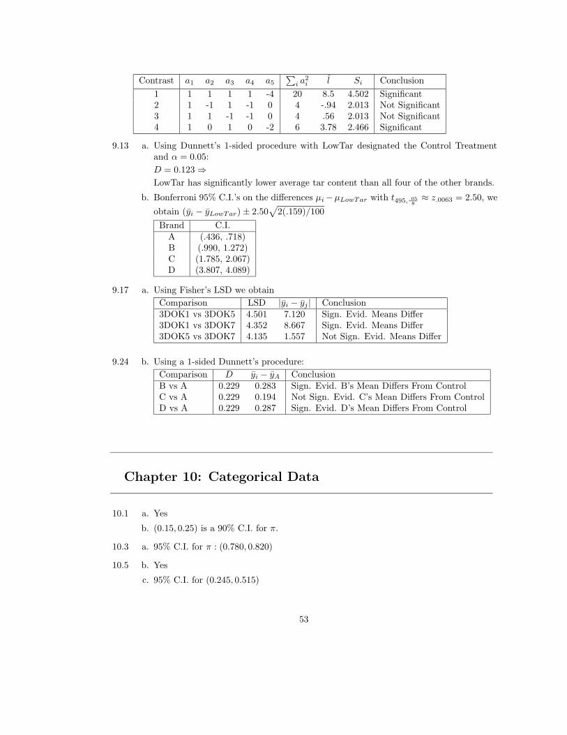
Contrast a1 a2 a3 a4 a5
∑i a
2i l Si Conclusion
1 1 1 1 1 -4 20 8.5 4.502 Significant2 1 -1 1 -1 0 4 -.94 2.013 Not Significant3 1 1 -1 -1 0 4 .56 2.013 Not Significant4 1 0 1 0 -2 6 3.78 2.466 Significant
9.13 a. Using Dunnett’s 1-sided procedure with LowTar designated the Control Treatmentand α = 0.05:
D = 0.123⇒LowTar has significantly lower average tar content than all four of the other brands.
b. Bonferroni 95% C.I.’s on the differences µi−µLowTar with t495, .058≈ z.0063 = 2.50, we
obtain (yi − yLowTar)± 2.50√
2(.159)/100
Brand C.I.A (.436, .718)B (.990, 1.272)C (1.785, 2.067)D (3.807, 4.089)
9.17 a. Using Fisher’s LSD we obtain
Comparison LSD |yi − yj | Conclusion3DOK1 vs 3DOK5 4.501 7.120 Sign. Evid. Means Differ3DOK1 vs 3DOK7 4.352 8.667 Sign. Evid. Means Differ3DOK5 vs 3DOK7 4.135 1.557 Not Sign. Evid. Means Differ
9.24 b. Using a 1-sided Dunnett’s procedure:
Comparison D yi − yA ConclusionB vs A 0.229 0.283 Sign. Evid. B’s Mean Differs From ControlC vs A 0.229 0.194 Not Sign. Evid. C’s Mean Differs From ControlD vs A 0.229 0.287 Sign. Evid. D’s Mean Differs From Control
Chapter 10: Categorical Data
10.1 a. Yes
b. (0.15, 0.25) is a 90% C.I. for π.
10.3 a. 95% C.I. for π : (0.780, 0.820)
10.5 b. Yes
c. 95% C.I. for (0.245, 0.515)
53
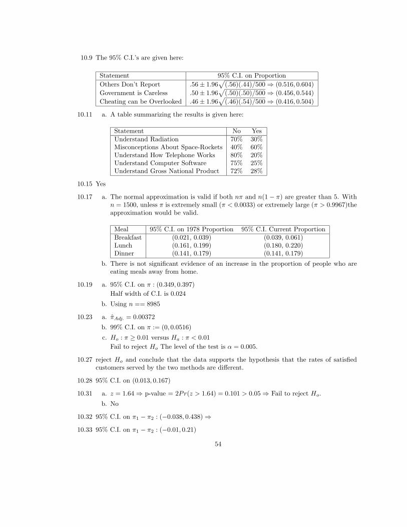
10.9 The 95% C.I.’s are given here:
Statement 95% C.I. on Proportion
Others Don’t Report .56± 1.96√
(.56)(.44)/500⇒ (0.516, 0.604)
Government is Careless .50± 1.96√
(.50)(.50)/500⇒ (0.456, 0.544)
Cheating can be Overlooked .46± 1.96√
(.46)(.54)/500⇒ (0.416, 0.504)
10.11 a. A table summarizing the results is given here:
Statement No YesUnderstand Radiation 70% 30%Misconceptions About Space-Rockets 40% 60%Understand How Telephone Works 80% 20%Understand Computer Software 75% 25%Understand Gross National Product 72% 28%
10.15 Yes
10.17 a. The normal approximation is valid if both nπ and n(1− π) are greater than 5. Withn = 1500, unless π is extremely small (π < 0.0033) or extremely large (π > 0.9967)theapproximation would be valid.
Meal 95% C.I. on 1978 Proportion 95% C.I. Current ProportionBreakfast (0.021, 0.039) (0.039, 0.061)Lunch (0.161, 0.199) (0.180, 0.220)Dinner (0.141, 0.179) (0.141, 0.179)
b. There is not significant evidence of an increase in the proportion of people who areeating meals away from home.
10.19 a. 95% C.I. on π : (0.349, 0.397)
Half width of C.I. is 0.024
b. Using n == 8985
10.23 a. πAdj. = 0.00372
b. 99% C.I. on π := (0, 0.0516)
c. Ho : π ≥ 0.01 versus Ha : π < 0.01
Fail to reject Ho The level of the test is α = 0.005.
10.27 reject Ho and conclude that the data supports the hypothesis that the rates of satisfiedcustomers served by the two methods are different.
10.28 95% C.I. on (0.013, 0.167)
10.31 a. z = 1.64⇒ p-value = 2Pr(z > 1.64) = 0.101 > 0.05⇒ Fail to reject Ho.
b. No
10.32 95% C.I. on π1 − π2 : (−0.038, 0.438)⇒
10.33 95% C.I. on π1 − π2 : (−0.01, 0.21)
54
10.35 a. z = 9.54⇒ p− value = Pr(z > 9.54) < 0.0001
Reject Ho
10.43 Ho : π1 = 13 , π2 = 1
3 , π3 = 13
Ha : at least on of the groups had probability of interning different from 13
χ2 = 6.952 with df = 3− 1 = 2⇒ 0.025 < p− value < 0.05⇒Fail to reject Ho.
10.45 Ho : π1 = 0.50, π2 = 0.40, π3 = 0.10
Ha : at least on of the πis differs from its hypothesized value
χ2 = 6.0 with df = 3− 1 = 2⇒ 0.025 < p− value < 0.05⇒Reject Ho
10.47 Ho : π1 = 0.25, π2 = 0.25, π3 = 0.25, π4 = 0.25
Ha : at least on of the πis differs from 0.25
χ2 = 123.70 with df = 4− 1 = 3⇒ p− value < 0.001⇒Reject Ho.
10.49 Ho : π1 = 0.25, π2 = 0.25, π3 = 0.25, π4 = 0.25
Ha : at least on of the πis differs from its hypothesized value
χ2 = 2.4 with df = 4− 1 = 3⇒ p− value > 0.10⇒Fail to reject Ho.
10.51 a. The probabilities are given here:
µ 0.5 1.0 3.0P (y = 1) 0.3033 0.3679 0.1494
b. The probabilities are given here:
µ 1.7 2.5 4.2P (y > 1) 0.5067 0.7127 0.9220
c. The probabilities are given here:
µ 0.2 1.0 2.0P (y < 5) 1.0 0.9964 0.9476
10.53 a. P (y < 6) =∑5k=0
250!k!(250−k)! (0.01)k(1− 0.01)250−k
c. P (y < 6) ≈ P (z < 1.91) = 0.9719
d. P (y < 6) ≈ 0.9580
10.55 a. Yes, the Poisson conditions appear to be reasonably satisfied in this situation.
55

b. Ho : µ = 2 versus Ha : µ 6= 2
Using µ = 2.0, the Poisson table yields the following probabilities:
k 0 1 2 3 4 5 ≥ 6πi = P (y = k) 0.1353 0.2707 0.2702 0.1804 0.0902 0.0361 0.0166Ei = 800πi 108.24 216.56 216.56 144.32 72.16 28.88 13.28
χ2 = 8.272 with df = 7− 1 = 6⇒ p− value > 0.10⇒Fail to reject Ho.
10.57 a. From the data y ≈ 1100
∑i(ni)(yi) = 5.57
s2 ≈ 199
∑i ni(yi − 5.57)2 = 1056.5/99 = 10.67
b. Using µ = 5.5, the Poisson table yields the following probabilities
k ≤ 1 2 3 4 5 6πi = P (y = k) 0.0266 0.0618 0.1133 0.1558 0.1714 0.1571Ei = 100πi 2.66 6.18 11.33 15.58 17.14 15.71k 7 8 ≥ 9πi = P (y = k) 0.1234 0.0849 0.1057Ei = 100πi 12.34 8.49 10.57
χ2 = 13.441 with df = 9− 2 = 7⇒ 0.05 < p− value < 0.10⇒Fail to reject Ho.
10.60 a. The expected counts are displayed in the following table:
ColumnRow 1 2 3 41 16.0 22.4 25.6 16.02 34.0 47.6 54.4 34.0
b. df = (2-1)(4-1) = 3
c. Using the chi-square approximation with df = 3 and χ2 = 13.025,
⇒ 0.001 < p− value < 0.005.
10.61 0.001 < p− value < 0.005
10.67 a. Under the hypothesis of independence, the expected frequencies are given in the fol-lowing table
OpinionCommercial 1 2 3 4 5A 42 107 78 34 39B 42 107 78 34 39C 42 107 78 34 39
b. df = (3-1)(5-1) = 8
56
c. The cell chi-squares are given in the following table:
OpinionCommercial 1 2 3 4 5A 2.3810 3.7383 2.1667 4.2353 0.6410B 2.8810 10.8037 0.0513 5.7647 21.5641C 0.0238 1.8318 1.5513 0.1176 14.7692
χ2 = 72.521 with df = 8⇒ p− value = P (χ2 > 72.521) < 0.001⇒Reject Ho.
10.68 With df = 8, p− value = P (χ2 > 72.521) < 0.001
10.69 The relevant proportions are given in the following table:
OpinionCommercial 1 2 3 4 5 TotalA 0.1067 0.2900 0.3033 0.1533 0.1467 1.0B 0.1767 0.4700 0.2533 0.0667 0.0333 1.0C 0.1367 0.3100 0.2233 0.1200 0.2100 1.0Total 0.1400 0.3567 0.2600 0.1133 0.1300 1.0
λ=(579-575)/579=0.0069.
10.73 b. The goodness-of-fit test is computed in the following table:
Selection Theoretical Expected Observed CellRating Proportions Frequencies Frequencies chi-square:
πi Ei = 216πi ni (ni − Ei)2/Ei1 0.25 54 11 34.24072 0.25 54 30 10.66673 0.25 54 88 21.404744 0.25 54 87 20.1667Total 1.00 216 216 86.4815
Ho : π1 = 0.25, π2 = 0.25, π3 = 0.25, π4 = 0.25 versus
Ha : Selection Rating categories are not equally likely
χ2 = 86.4815 with df = 4− 1 = 3⇒ p− value < 0.001⇒Reject Ho.
10.74 a. The initial analysis of the data yielded a contingency table with 5 of the 16 cells (31%)having expected values less than 5. The first two levels of the adequacy rating werecombined. The following SAS output was then obtained.
57

SAS System:
The FREQ Procedure
Table of Adequacy Rating by Frequency
Adequacy Rating| Frequency
|
Frequency |
Expected |
Cell Chi-Square|
Percent |
Row Pct | | | | |
Col Pct | 1| 2| 3| 4| Total
------------------------------------------------------------
1 | 5 | 8 | 11 | 17 | 41
| 16.324 | 12.718 | 7.5926 | 4.3657 |
| 7.8556 | 1.75 | 1.5292 | 36.563 |
| 2.31 | 3.70 | 5.09 | 7.87 | 18.98
| 12.20 | 19.51 | 26.83 | 41.46 |
| 5.81 | 11.94 | 27.50 | 73.91 |
------------------------------------------------------------
3 | 37 | 30 | 16 | 5 | 88
| 35.037 | 27.296 | 16.296 | 9.3704 |
| 0.11 | 0.2678 | 0.0054 | 2.0384 |
| 17.13 | 13.89 | 7.41 | 2.31 | 40.74
| 42.05 | 34.09 | 18.18 | 5.68 |
| 43.02 | 44.78 | 40.00 | 21.74 |
------------------------------------------------------------
4 | 44 | 29 | 13 | 1 | 87
| 34.639 | 26.986 | 16.111 | 9.2639 |
| 2.5298 | 0.1503 | 0.6008 | 7.3718 |
| 20.37 | 13.43 | 6.02 | 0.46 | 40.28
| 50.57 | 33.33 | 14.94 | 1.15 |
| 51.16 | 43.28 | 32.50 | 4.35 |
-------------------------------------------------------------
Total | 86 67 40 23 | 216
| 39.81 31.02 18.52 10.65 | 100.00
Statistics for Table of Adequacy Rating by Frequency
Statistic DF Value Prob
-------------------------------------------------------
Chi-Square 6 60.7719 <.0001
Likelihood Ratio Chi-Square 6 53.1543 <.0001
Mantel-Haenszel Chi-Square 1 46.7048 <.0001
Phi Coefficient 0.5304
Contingency Coefficient 0.4686
Cramer’s V 0.3751
Sample Size = 216
conclude that there is some relation between the two variables.
10.78 a. Control: 10%; Low Dose 14%; High Dose 19%
b. Ho : π1 = π2 = π3 versus Ha : The proportions are not all equal,
58
where πj is probability of a rat in Group j having One or More Tumors.
χ2 = 3.312 with df = (2-1)(3-1) = 2 and p-value = 0.191.
c. No
10.81 a. The results are summarized in the following table:
Question π σπ 95% C.I.Did Not Explain? 0.254 0.01947 (0.216, 0.292)Might Bother? 0.916 0.0124 (0.892, 0.940)Did Not Ask? 0.471 0.02232 (0.427, 0.515)Drug Not Changed? 0.877 0.0147 (0.848, 0.906)
10.85 y =∑i(No.Mites)(frequency)/500 = 1.146
we obtain the following using a Poisson distribution with µ = 1.2:
Mites/Leaf (ki) 0 1 2 3 4 ≥ 5 Totalπi = P (y = ki) 0.3012 0.3614 0.2169 0.0867 0.0260 0.0078 1.0Ei = 500πi 150.6 180.7 108.5 43.3 13 3.9 500ni 233 127 57 33 30 20 500
χ2 = 176.6 with df =6-1 = 5, ⇒ p− value = Pr(χ2 > 176.6) < 0.001⇒Reject Ho
Chapter 11: Linear Regression and Correlation
11.3 The calculations are give here:
i xi yi (xi − 3)2 (xi − 3)(yi − 5.6)1 1 2 4 7.22 2 4 1 1.63 3 6 0 04 4 7 1 1.45 5 9 4 6.8
Total 15 28 10 17
x = 15/5 = 3 y = 28/5 = 5.6
Sxx =∑i(xi − 3)2 = 10
Sxy =∑i(xi − 3)(yi − 5.6) = 17
β1 = Sxy/Sxx = 17/10 = 1.7
β0 = y − β1x = 5.6− (1.7)(3) = 0.5
59

y = 0.5 + 1.7x
11.5 β1 = 1.633
β0 = 2.468
y = 2.468 + 1.633x
11.9 a. A scatterplot of the data is given here:
••
•
•
•
•
•
•
••
Effect of Exposure Time on Fish Quality
Time After Capture
Fish
Qua
lity
0 1 2 3 4 5 6 7 8 9 10 11 12
5.0
5.5
6.0
6.5
7.0
7.5
8.0
8.5
9.0
9.5
10.0
b. Minitab output is given here:
Regression Analysis: QUALITY versus STORAGE
The regression equation is
QUALITY = 8.46 - 0.142 STORAGE
Predictor Coef SE Coef T P
Constant 8.46000 0.06610 127.99 0.000
STORAGE -0.141667 0.008995 -15.75 0.000
S = 0.1207 R-Sq = 96.9% R-Sq(adj) = 96.5%
Analysis of Variance
Source DF SS MS F P
Regression 1 3.6125 3.6125 248.07 0.000
Residual Error 8 0.1165 0.0146
60
Total 9 3.7290
The least squares estimates are β0 = 8.46 and β1 = −0.142
c. The estimated slope value β1 = −0.142 indicates that for each 1 hour increase in thetime between the capture of the fish and their placement in storage there is approxi-mately a 0.142 decrease in the average quality of the fish.
11.10 y = 8.46− 0.142x ⇒ y = 8.46− 0.142(10) = 7.04
It would not be a good idea to make predictions at x = 18
11.15 logarithmic transformation is suggested from the plot.
11.16 a. For the transformed data, the plotted points appear to be reasonably linear.
b. The least squares line is y = 3.10 + 2.76√x
(Using rounded values 3.097869 ≈ 3.10 and 2.7633138 ≈ 2.76).
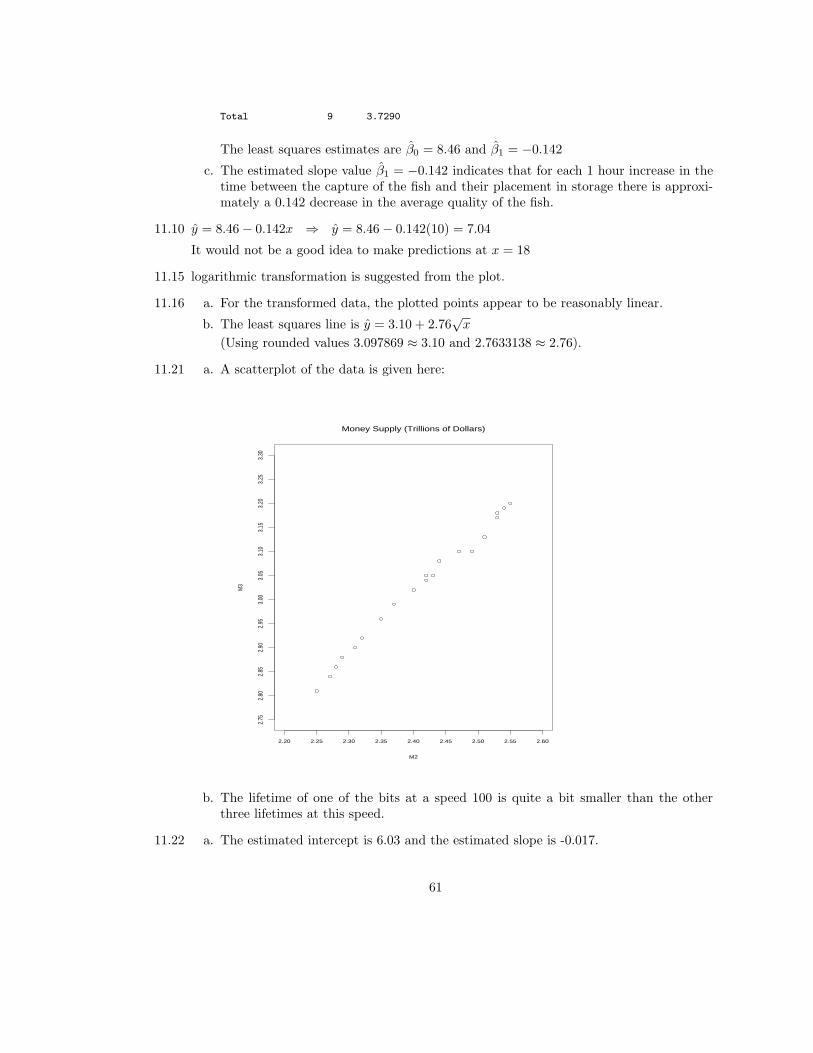
11.21 a. A scatterplot of the data is given here:
Money Supply (Trillions of Dollars)
M2
M3
2.20 2.25 2.30 2.35 2.40 2.45 2.50 2.55 2.60
2.75
2.80
2.85
2.90
2.95
3.00
3.05
3.10
3.15
3.20
3.25
3.30
b. The lifetime of one of the bits at a speed 100 is quite a bit smaller than the otherthree lifetimes at this speed.
11.22 a. The estimated intercept is 6.03 and the estimated slope is -0.017.
61

b. The slope has a negative sign which indicates a decreasing relation between lifetimeand speed.
c. 0.6324.
11.23 a. The prediction equation is y = 6.03− 0.017x. Thus, we just replace x with the speedsof 60, 80, 100, 120, and 140 to obtain the values:
x = 60⇒ y = 5.01
x = 80⇒ y = 4.67
x = 100⇒ y = 4.33
x = 120⇒ y = 3.99
x = 140⇒ y = 3.65
11.29 Minitab output is given here:
Regression Analysis: FIRMNESS versus CONCENTRATION
The regression equation is
FIRMNESS = 48.9 + 10.3 CONCENTRATION
Predictor Coef SE Coef T P
Constant 48.933 1.541 31.76 0.000
CONCENTR 10.3333 0.7957 12.99 0.000
S = 2.387 R-Sq = 97.7% R-Sq(adj) = 97.1%
Analysis of Variance
Source DF SS MS F P
Regression 1 961.00 961.00 168.65 0.000
Residual Error 4 22.79 5.70
Total 5 983.79
a. y = 48.9 + 10.3x
b. S2 = 5.70
c. SE(β1) = 0.7957
11.30 Ho : β1 = 0 versus Ha : β1 6= 0
Test Statistic: t = β1
se/Sxx= 10.33
2.387/9 = 12.99
p− value = 2P (t4 > 12.99) < 0.0001⇒ Reject Ho
11.35 a. Yes
b. y = 12.51 + 35.83x
11.36 a. 1.069
b. 6.957
62
c. Ho : β1 ≤ 0 versus Ha : β1 > 0
Test Statistic: t = 5.15
p − value = P (t10 > 5.15) = 0.0002 ⇒ Reject Ho and conclude there is significantevidence that there is a positive linear relationship.
11.37 a. No
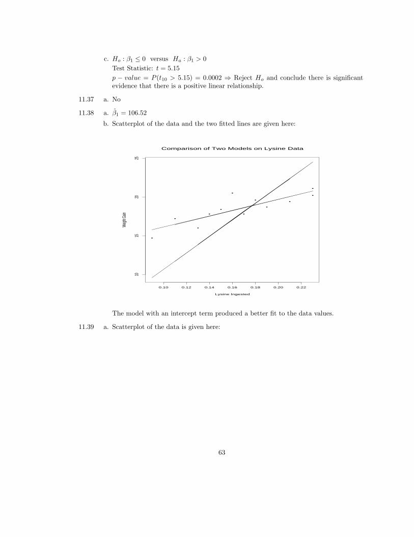
11.38 a. β1 = 106.52
b. Scatterplot of the data and the two fitted lines are given here:
Comparison of Two Models on Lysine Data
Lysine Ingested
Weigh
t Gain
0.10 0.12 0.14 0.16 0.18 0.20 0.22
1015
2025
•
•
•
•
•
•
•
•
•
•
•
•
The model with an intercept term produced a better fit to the data values.
11.39 a. Scatterplot of the data is given here:
63

•
•
•
••
•
•
•••
•
•
••
•
•
•
•
••
••••
•
•
•
•
•
•
Total Direct Cost versus Run Size
Run Size
Total
Cost
0 1 2 3 4 5 6 7 8 9 11 13 15 17 19
100
200
300
400
500
600
700
800
900
1000
1100
1200
b. y = 99.777 + 5.1918x
The residual standard deviation is s = 12.2065
c. A 95% C.I. for the slope is given by (5.072, 5.312)
11.43 95% prediction interval for log biological recovery percentage at x=30 is given by (0.941,1.449)
11.44 a. y = −1.733333 + 1.316667x
b. The p-value for testing Ho : β1 ≤ 0 versus Ha : β1 > 0 is
p− value = P (t10 ≥ 6.342) < 0.0005⇒ Reject Ho
11.45 a. 95% Confidence Intervals for E(y) at selected values for x:
x = 4⇒ (2.6679, 4.3987)
x = 5⇒ (4.2835, 5.4165)
x = 6⇒ (5.6001, 6.7332)
x = 7⇒ (6.6179, 8.3487)
b. 95% Prediction Intervals for y at selected values for x :
x = 4⇒ (1.5437, 5.5229)
x = 5⇒ (2.9710, 6.7290)
x = 6⇒ (4.2877, 8.0456)
x = 7⇒ (5.4937, 9.4729)
11.46 a. y = 99.77704 + 51.9179x⇒ When x=2.0, E(y) = 203.613
b. The 95% C.I. is given in the output as (198.902, 208.323)
64
11.47 No
11.48 a. The 95% P.I. is given in the output as (178.169, 229.057)
b. Yes
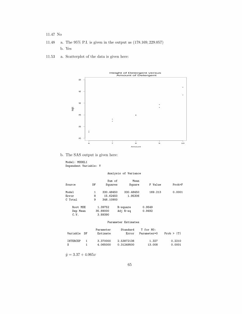
11.53 a. Scatterplot of the data is given here:
••
•
•
••
•
•
•
•
Height of Detergent versus Amount of Detergent
Amount
Heigh
t
6 7 8 9 10
2530
3540
4550
b. The SAS output is given here:
Model: MODEL1
Dependent Variable: Y
Analysis of Variance
Sum of Mean
Source DF Squares Square F Value Prob>F
Model 1 330.48450 330.48450 169.213 0.0001
Error 8 15.62450 1.95306
C Total 9 346.10900
Root MSE 1.39752 R-square 0.9549
Dep Mean 35.89000 Adj R-sq 0.9492
C.V. 3.89390
Parameter Estimates
Parameter Standard T for H0:
Variable DF Estimate Error Parameter=0 Prob > |T|
INTERCEP 1 3.370000 2.53872138 1.327 0.2210
X 1 4.065000 0.31249500 13.008 0.0001
y = 3.37 + 4.065x
65
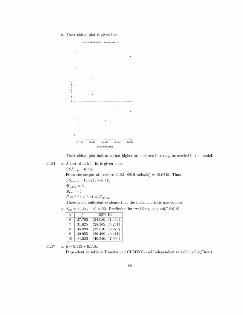
c. The residual plot is given here:
Plot of RESID*PRED. Symbol used is ’*’.
|
|
3 +
|
| *
|
|
|
|
2 +
|
|
|
| *
|
R |
E 1 +
S |
I |
D |
U | *
A | *
L |
S 0 +-----------------------------------------------------
| *
|
|
| * *
|
| *
-1 +
| *
|
|
|
| *
|
-2 +
|
---+-----------+-----------+-----------+-----------+--
27.760 31.825 35.890 39.955 44.020
PREDICTED VALUE
The residual plot indicates that higher order terms in x may be needed in the model.
11.54 a. A test of lack of fit is given here:
SSPexp = 6.715
From the output of exercise 11.53, SS(Residuals) = 15.6245. Thus,
SSLack = 15.6245− 6.715
dfLack = 3
dfexp = 5
F = 2.21 < 5.41 = F.05,3,5
There is not sufficient evidence that the linear model is inadequate.
b. Sxx =∑i(xi − x) = 20. Prediction interval for y at x =6,7,8,9,10
x y 95% P.I.6 27.760 (24.086, 31.434)7 31.825 (28.369, 35.281)8 35.890 (32.510, 39.270)9 39.955 (36.499, 43.411)10 44.020 (40.346, 47.694)
11.57 a. y = 0.113 + 0.118x
Dependent variable is Transformed CUMVOL and Independent variable is Log(Dose).
66

b. x = (y − 0.11277)/0.11847
xL = 2.40 + 1(1−.2426) (x− 2.40− d)
xU = 2.40 + 1(1−.2426) (x− 2.40 + d)⇒
y TRANS(y) ˆLOG(x) x d ˆLOG(x)LˆLOG(x)U xL xU
10 .322 1.764 5.84 .242289 1.24038 1.88018 3.46 6.5514 .383 2.285 9.83 .198634 1.98616 2.51068 7.29 12.3119 .451 2.855 17.38 .221359 2.70876 3.29328 15.01 26.93
11.58 The four values of CUMVOL are 10, 20, 30, 12 yielding y = 0.42969 and sy = .05849,where y is the arcsine of the square root of CUMVOL.
For 50%: x = 2.367 and 95% confidence limits are (0.79, 4.45)
For 75%: x = 5.861 and 95% confidence limits are (2.20, 12.88)
11.59 r = 0.9722.
11.60 a. Test Ho : ρyx ≤ 0 versus Ha : ρyx > 0
Test Statistic: t13.13
p− value < 0.0005
Conclusion: There is significant evidence that the correlation is positive.
11.61 a. r2yx = 99.64% (R-squared on output).
b. ryx should be positive.
11.63 a. There appears to be a general increase in salary as the level of experience increases.
11.65 a. y = 40.507 + 1.470x
b. The residual standard deviation is sε = 5.402.
c. From the output t = 6.916 with a p-value of 0.000. This would imply overwhelmingevidence that there is a relation between starting salary and experience.
d. R2 = 0.494
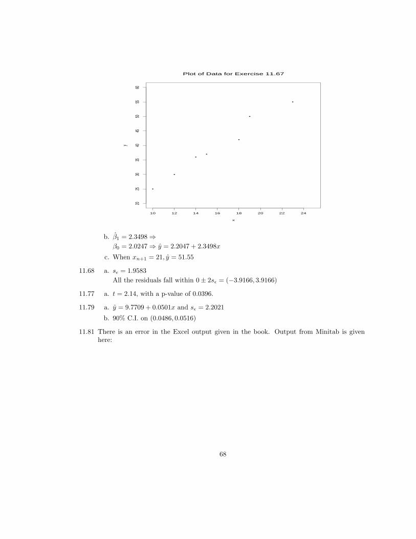
11.67 a. Scatterplot of the data is given here:
67
•
•
••
•
•
•
Plot of Data for Exercise 11.67
x
y
10 12 14 16 18 20 22 24
2025
3035
4045
5055
60
b. β1 = 2.3498⇒β0 = 2.0247⇒ y = 2.2047 + 2.3498x
c. When xn+1 = 21, y = 51.55
11.68 a. sε = 1.9583
All the residuals fall within 0± 2sε = (−3.9166, 3.9166)
11.77 a. t = 2.14, with a p-value of 0.0396.
11.79 a. y = 9.7709 + 0.0501x and sε = 2.2021
b. 90% C.I. on (0.0486, 0.0516)
11.81 There is an error in the Excel output given in the book. Output from Minitab is givenhere:
68

Regression Analysis: Rate: versus Mileage:
The regression equation is
Rate: = 9.79 + 0.0503 Mileage:
Predictor Coef SE Coef T P
Constant 9.7932 0.4391 22.30 0.000
Mileage: 0.0503229 0.0008230 61.14 0.000
S = 2.042 R-Sq = 98.8% R-Sq(adj) = 98.8%
Analysis of Variance
Source DF SS MS F P
Regression 1 15590 15590 3738.63 0.000
Residual Error 46 192 4
Total 47 15782
Predicted Values for New Observations
New Obs Fit SE Fit 95.0% CI 95.0% PI
1 26.903 0.298 ( 26.303, 27.503) ( 22.749, 31.057)
Values of Predictors for New Observations
New Obs Mileage:
1 340
y = 26.903
The 95% P.I. when x=340 is (22.749, 31.057)
11.87 The Minitab output is given here:
Regression Analysis: Yield versus Nitrogen
The regression equation is
Yield = 11.8 + 6.50 Nitrogen
Predictor Coef SE Coef T P
Constant 11.778 1.887 6.24 0.000
Nitrogen 6.5000 0.8736 7.44 0.000
S = 2.140 R-Sq = 88.8% R-Sq(adj) = 87.2%
Analysis of Variance
Source DF SS MS F P
Regression 1 253.50 253.50 55.36 0.000
Residual Error 7 32.06 4.58
Lack of Fit 1 2.72 2.72 0.56 0.484
Pure Error 6 29.33 4.89
Total 8 285.56
69
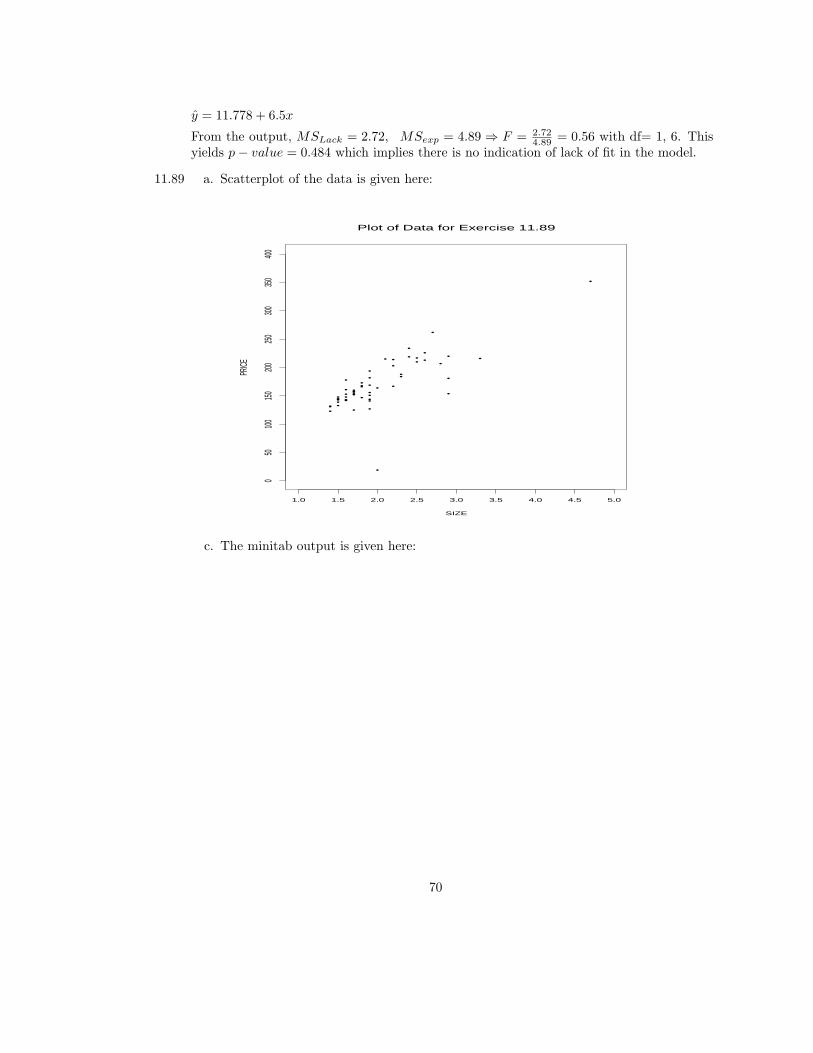
y = 11.778 + 6.5x
From the output, MSLack = 2.72, MSexp = 4.89⇒ F = 2.724.89 = 0.56 with df= 1, 6. This
yields p− value = 0.484 which implies there is no indication of lack of fit in the model.
11.89 a. Scatterplot of the data is given here:
•
•
•
•
•
•
• ••
•
•
•
•
•
•
•
•
•
•
•
•• ••
•
•
•
•
•
•
•
•
••
• ••
•
•
••
•
••
•
•
•
•
•
•
•
•
•
•
•
•
Plot of Data for Exercise 11.89
SIZE
PRICE
1.0 1.5 2.0 2.5 3.0 3.5 4.0 4.5 5.0
050
100
150
200
250
300
350
400
c. The minitab output is given here:
70
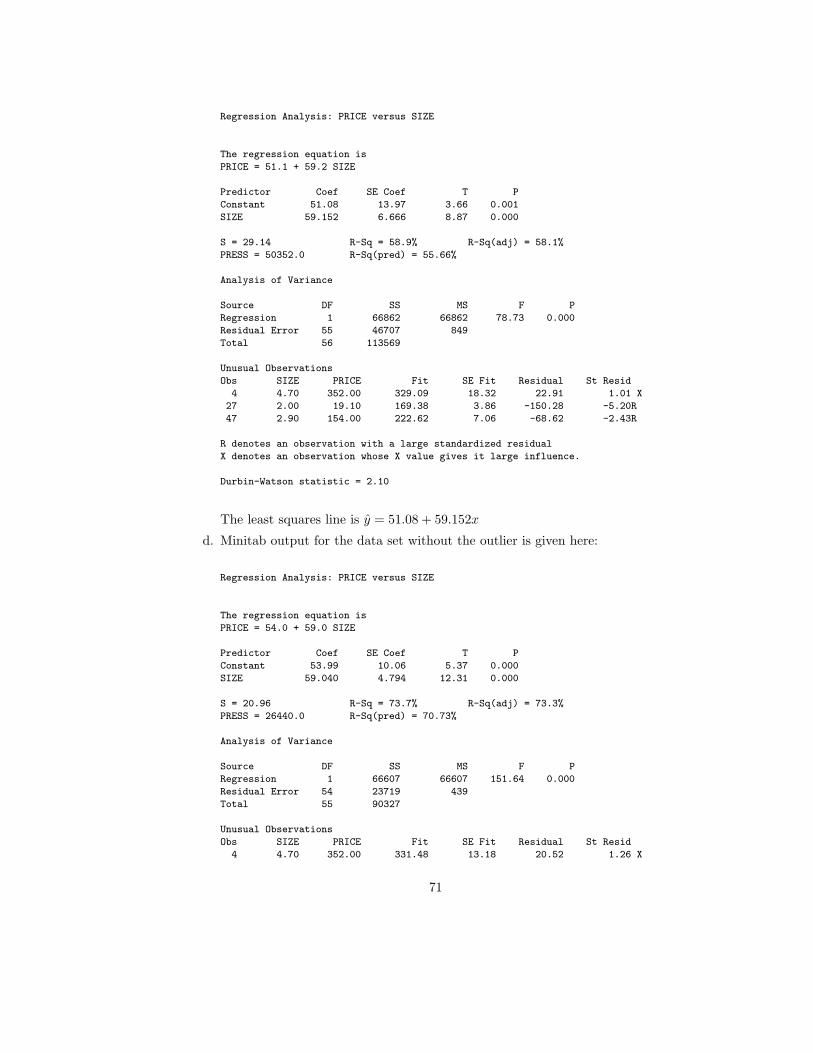
Regression Analysis: PRICE versus SIZE
The regression equation is
PRICE = 51.1 + 59.2 SIZE
Predictor Coef SE Coef T P
Constant 51.08 13.97 3.66 0.001
SIZE 59.152 6.666 8.87 0.000
S = 29.14 R-Sq = 58.9% R-Sq(adj) = 58.1%
PRESS = 50352.0 R-Sq(pred) = 55.66%
Analysis of Variance
Source DF SS MS F P
Regression 1 66862 66862 78.73 0.000
Residual Error 55 46707 849
Total 56 113569
Unusual Observations
Obs SIZE PRICE Fit SE Fit Residual St Resid
4 4.70 352.00 329.09 18.32 22.91 1.01 X
27 2.00 19.10 169.38 3.86 -150.28 -5.20R
47 2.90 154.00 222.62 7.06 -68.62 -2.43R
R denotes an observation with a large standardized residual
X denotes an observation whose X value gives it large influence.
Durbin-Watson statistic = 2.10
The least squares line is y = 51.08 + 59.152x
d. Minitab output for the data set without the outlier is given here:
Regression Analysis: PRICE versus SIZE
The regression equation is
PRICE = 54.0 + 59.0 SIZE
Predictor Coef SE Coef T P
Constant 53.99 10.06 5.37 0.000
SIZE 59.040 4.794 12.31 0.000
S = 20.96 R-Sq = 73.7% R-Sq(adj) = 73.3%
PRESS = 26440.0 R-Sq(pred) = 70.73%
Analysis of Variance
Source DF SS MS F P
Regression 1 66607 66607 151.64 0.000
Residual Error 54 23719 439
Total 55 90327
Unusual Observations
Obs SIZE PRICE Fit SE Fit Residual St Resid
4 4.70 352.00 331.48 13.18 20.52 1.26 X
71

13 2.90 181.00 225.20 5.09 -44.20 -2.17R
26 2.70 262.00 213.40 4.32 48.60 2.37R
46 2.90 154.00 225.20 5.09 -71.20 -3.50R
R denotes an observation with a large standardized residual
X denotes an observation whose X value gives it large influence.
Durbin-Watson statistic = 1.83
Predicted Values for New Observations
New Obs Fit SE Fit 95.0% CI 95.0% PI
1 349.19 14.59 ( 319.94, 378.43) ( 297.99, 400.38) XX
X denotes a row with X values away from the center
XX denotes a row with very extreme X values
Values of Predictors for New Observations
New Obs SIZE
1 5.00
y = 53.99 + 59.04x.
e. The residual standard deviations are sε = 29.14 with outlier and sε = 20.96 withoutoutlier.
11.90 a. The estimated intercept is βo = 53.99.
c. Using the estimates from the Minitab output, a 95% C.I. for β1 is (49.428, 68.652).
11.91 a. From the Minitab output, a 95% P.I. for the selling price when the size is 5:
(297.99, 400.38).
b. Scatterplot of the data is given here:
•
•
•
•
•
•
• ••
•
•
•
•
•
•
•
•
•
•
•
•• ••
•
•
•
•
•
•
•
••
• ••
•
•
••
•
••
•
•
•
•
•
•
•
•
•
•
•
•
Plot of Data for Exercise 11.91
SIZE
PRICE
1.0 1.5 2.0 2.5 3.0 3.5 4.0 4.5 5.0
050
100
150
200
250
300
350
400
72

c. The P.I. may not be valid since the statistical procedures depend on the conditionthat the variance remain constant across the range of x-values.
11.96 Minitab output is given here:
Regression Analysis: DURABIL versus CONCENTR
The regression equation is
DURABIL = 47.0 + 0.308 CONCENTR
Predictor Coef SE Coef T P
Constant 47.020 4.728 9.94 0.000
CONCENTR 0.3075 0.1114 2.76 0.008
S = 12.21 R-Sq = 11.6% R-Sq(adj) = 10.1%
PRESS = 9368.62 R-Sq(pred) = 4.20%
Analysis of Variance
Source DF SS MS F P
Regression 1 1134.7 1134.7 7.61 0.008
Residual Error 58 8644.5 149.0
Total 59 9779.2
Unusual Observations
Obs CONCENTR DURABIL Fit SE Fit Residual St Resid
2 20.0 25.20 53.17 2.73 -27.97 -2.35R
4 20.0 20.30 53.17 2.73 -32.87 -2.76R
60 60.0 18.90 65.47 2.73 -46.57 -3.91R
R denotes an observation with a large standardized residual
Durbin-Watson statistic = 1.35
a. y = 47.020 + 0.3075x. The estimated slope β1 = 0.3075 can be interpreted as follows:there is a 0.3075 increase in average durability for a 1 unit increase in the concentration.
b. The coefficient of determination, R2 = 11.6%.
11.97 For testing Ho : β1 = 0 versus Ha : β1 6= 0, t = 2.76 with p− value = 0.008. The p-value isless than α = 0.01 thus we reject Ho
11.98 Scatterplot of the data is given here:
73

•
•
•
•
•
•
•
•
•
•
•
•
••
•
•
•
•
•
••
•
••
•
•
•
••
•
•
••
••
•
•
•
•
•
•
•
•
•
••
•
•
•
•
•
•
•
••
••
•
•
•
Plot of Durability vs Concentration
CONCENTRATION
DURA
BILITY
20 24 28 32 36 40 44 48 52 56 60 64
2025
3035
4045
5055
6065
7075
80
a. From the scatterplot, there is a definite curvature in the relation between Durabilityand Concentration. A straight-line model would not appear to be appropriate.
b. The coefficient of determination, R2, measures the strength of the linear (straight-line) relation only. A straight-line model does not adequately describe the relationbetween Durability and Concentrtation. This is indicated by the small percentage ofthe variation, 11.6%, in the values of Durability explained by the model containingjust a linear relation with Concentration.
Chapter 12: Multiple Regression and
the General Linear Model
12.1 a. yj = µij + εj , with ij = 1, 2, · · · , 12
b. x1 =
{1 if V1 = 1st Level0 if Otherwise
x2 =
{1 if V2 = 1st Level0 if Otherwise
x3 =
{1 if V2 = 2nd Level0 if Otherwise
x4 =
{1 if V3 = 1st Level0 if Otherwise
74

yj = βo + β1x1j + β2x2j + β3x3j + β4x4j + εj , with j = 1, · · · , n
12.3 The model is given here:
yi = β0 + β1x1i + β2x2i + β3x3i + β4x4i + β5x5i + β6x6i + β7x7i + β8x8i + β9x9i + εi
with x1 = x1, x2 = x2, x3 = x3, x4 = x21, x5 = x2
2,
x6 = x23, x7 = x1x2, x8 = x1x3, x9 = x2x3
12.5 a. For the model of the ith observation in the experiment:
yi = βo + β1x1i + β2x2i + β3x3i + εi,
µjk, the mean of the population consisting of Treatment #j and Location #k; j =1, 2, 3; k = 1, 2 :
LocationTreatment 1 2
1 µ11 = βo µ12 = βo + β3
2 µ21 = βo + β1 µ22 = βo + β1 + β3
3 µ31 = βo + β2 µ32 = βo + β2 + β3
We can thus interpret the β′s as follows:
βo = µ11, mean of TRT #1, LOC #1
β1 = µ21 − µ11 or β1 = µ22 − µ12,
difference of mean of TRT #2 and TRT #1 at a given Location
β2 = µ31 − µ11 or β2 = µ32 − µ12,
difference of mean of TRT #3 and TRT #1 at a given Location
β3 = µ12 − µ11 or β3 = µ22 − µ21 or β3 = µ32 − µ31,
difference of mean of LOC #2 and LOC #1 for a given Treatment
b. µ22 − µ32 = (β0 + β1 + β3)− (β0 + β2 + β3) = β1 − β2
Yes, the difference is the same for Location #1.
12.7 a. A scatterplot of the data is given here:
75

•
•
•
•
•
••
••
••
•
••
•
Plot of Drug Potency versus Dose Level
Dose Level
Pote
ncy
0 5 10 15 20 25 30 35
05
1015
2025
30
b. y = 8.667 + 0.575x
12.8 a. The logarithm of the dose levels are given here:
Dose Level (x) 2 4 8 16 32ln(x) 0.693 1.386 2.079 2.773 3.466
A scatterplot of the data is given here:
76

•
•
•
•
•
••
••
••
•
••
•
Plot of Drug Potency versus Log Dose Level
Logarithm of Dose Level
Pote
ncy
0.5 1.0 1.5 2.0 2.5 3.0 3.5
05
1015
2025
30
b. y = 1.2 + 7.021ln(x)
12.9 a. y = 326.39 + 136.10 ∗ Promo− 61.18 ∗Devel − 43.70 ∗Researchb. sε =
√MS(Residual) =
√656.811614 = 25.628
12.17 a. MS(Regression) = 159.67 and MS(Residual) = 7.00
b. F = 22.81
c. p− value = Pr(F3,8 ≥ 22.81) < 0.0001
d. In testing Ho : β1 = β2 = β3 = β4 = 0 versus Ha : at least one βi 6= 0, the p-valueprovides strong evidence to reject Ho and conclude that the independent variablesx,w, and v, as a group, have at least some degree of relationship with the dependentvariable, y.
e. A 95% C.I. for β1 is given by β1 ± (t.025,8)(SE(β1)) ⇒ 5.000 ± (2.306)(6.895) ⇒(−10.90, 20.90)
12.20 The t-value is t.05,19 = 1.729⇒ 90% C.I.’s for βi are given by:
Air Miles: (0.0841, 0.5003)
Population: (1.2302, 1.8319)
12.21 a. y = 7.20439+1.36291 METAL+0.30588 TEMP+0.01024 WATTS−0.00277 METXTEXP
77

b. The results of the various t-tests are given here:
Ho Ha T.S. t Conclusionβo = 0 βo 6= 0 t = 0.41 p− value = 0.6855 Fail to Reject Ho
β1 = 0 β1 6= 0 t = 1.47 p− value = 0.1559 Fail to Reject Ho
β2 = 0 β2 6= 0 t = 0.19 p− value = 0.8522 Fail to Reject Ho
β3 = 0 β3 6= 0 t = 2.16 p− value = 0.0427 Reject Ho
β4 = 0 β4 6= 0 t = −0.04 p− value = 0.9717 Fail to Reject Ho
c. t.025,20 = 2.086⇒ 95% C.I. on β4 is given by
−0.00277± (2.086)(0.07722)⇒ (−0.164, 0.158)
12.23 a. R2 = 0.6978
b. F = [SSReg.,Complete−SSReg.,Reduced]/(k−g)SSResidual,Complete/[n−(k+1)] = 3.12
with df = 2, 20⇒ p− value = Pr(F2,20 ≥ 3.12) = 0.066⇒Fail to reject Ho.
12.25 In the complete model, we want to test Ho : β1 = β2 = 0 versus Ha : β1 6= 0 and/or β2 6= 0.The F-statistic has the form:
F = [SSReg.,Complete−SSReg.,Reduced]/(k−g)SSResidual,Complete/[n−(k+1)] = 24.84
with df = 2, 17⇒ p− value = Pr(F2,17 ≥ 24.84) < 0.0001⇒Reject Ho.
12.28 a. y = 50.0195 + 6.64357x1 + 7.3145x2 − 1.23143x21 − 0.7724x1x2 − 1.1755x2
2
b. y = 70.31− 2.676x1 − 0.8802x2
c. For the Complete model: R2 = 86.24%
For the Reduced model: R2 = 58.85%
d. In the complete model, we want to test
Ho : β3 = β4 = β5 = 0 versus Ha : at least one of β3, β4, β5 6= 0.
The F-statistic has the form:
F = [SSReg.,Complete−SSReg.,Reduced]/(k−g)SSResidual,Complete/[n−(k+1)] = 9.29
with df = 3, 14⇒ p− value = Pr(F3,14 ≥ 9.29) = 0.0012⇒Reject Ho.
12.29 The predicted y-value at x=3, w=1, v=6 is y = 33.000 with 95% P.I.: (21.788, 44.212).
12.30 a. For the second order model, the 95% P.I. are
(54.7081, 65.1439) for x1 = 3.5 and x2 = 0.35
(57.0829, 67.6529) for x1 = 3.5 and x2 = 2.5
b. For the first order model, the 95% P.I. are
(50.0280, 65.6986) for x1 = 3.5 and x2 = 0.35
(51.0525, 66.4345) for x1 = 3.5 and x2 = 2.5
78
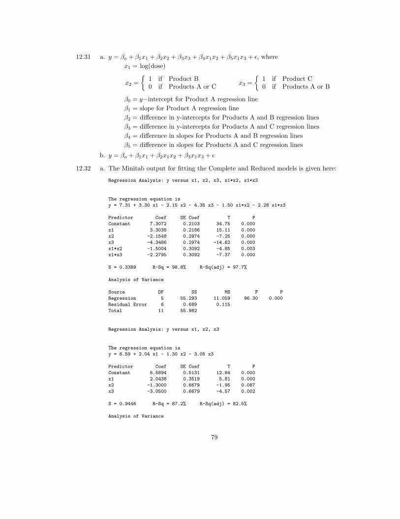
12.31 a. y = βo + β1x1 + β2x2 + β3x3 + β4x1x2 + β5x1x3 + ε, where
x1 = log(dose)
x2 =
{1 if Product B0 if Products A or C
x3 =
{1 if Product C0 if Products A or B
β0 = y−intercept for Product A regression line
β1 = slope for Product A regression line
β2 = difference in y-intercepts for Products A and B regression lines
β3 = difference in y-intercepts for Products A and C regression lines
β4 = difference in slopes for Products A and B regression lines
β5 = difference in slopes for Products A and C regression lines
b. y = βo + β1x1 + β2x1x2 + β3x1x3 + ε
12.32 a. The Minitab output for fitting the Complete and Reduced models is given here:
Regression Analysis: y versus x1, x2, x3, x1*x2, x1*x3
The regression equation is
y = 7.31 + 3.30 x1 - 2.15 x2 - 4.35 x3 - 1.50 x1*x2 - 2.28 x1*x3
Predictor Coef SE Coef T P
Constant 7.3072 0.2103 34.75 0.000
x1 3.3038 0.2186 15.11 0.000
x2 -2.1548 0.2974 -7.25 0.000
x3 -4.3486 0.2974 -14.62 0.000
x1*x2 -1.5004 0.3092 -4.85 0.003
x1*x3 -2.2795 0.3092 -7.37 0.000
S = 0.3389 R-Sq = 98.8% R-Sq(adj) = 97.7%
Analysis of Variance
Source DF SS MS F P
Regression 5 55.293 11.059 96.30 0.000
Residual Error 6 0.689 0.115
Total 11 55.982
Regression Analysis: y versus x1, x2, x3
The regression equation is
y = 6.59 + 2.04 x1 - 1.30 x2 - 3.05 x3
Predictor Coef SE Coef T P
Constant 6.5894 0.5131 12.84 0.000
x1 2.0438 0.3519 5.81 0.000
x2 -1.3000 0.6679 -1.95 0.087
x3 -3.0500 0.6679 -4.57 0.002
S = 0.9446 R-Sq = 87.2% R-Sq(adj) = 82.5%
Analysis of Variance
79

Source DF SS MS F P
Regression 3 48.844 16.281 18.25 0.001
Residual Error 8 7.138 0.892
Total 11 55.982
In the complete model: y = βo + β1x1 + β2x2 + β3x3 + β4x1x2 + β5x1x3 + ε, the testof equal slopes is a test of the hypotheses:
Ho : β4 = 0, β5 = 0 versus Ho : β4 6= 0 and/or β5 6= 0
Under Ho, the reduced model becomes y = βo + β1x1 + β2x2 + β3x3 + ε
F = 28.08⇒ p− value = Pr(F2,6 ≥ 28.08) = 0.0009⇒b. Reject Ho
c. In the complete model, a test of equal intercepts is a test of the hypotheses:
Ho : β2 = 0, β3 = 0 versus Ho : β2 6= 0 and/or β3 6= 0
Under Ho, reduced model becomes y = βo + β1x1 + β4x1x2 + β5x1x3 + ε
Obtain the SS’s from the reduced model and then conduct the F-test as was done inpart a.
12.33 a. For testing Ho : β1 = 0 versus Ha : β1 6= 0, the p-value for the output is p− value =0.0427. Thus, at the α = 0.05 level we can reject Ho
b. From the output, p(24) = 0.765 with 96% C.I. (0.437, 0.932).
12.35 a. y = −1.320 + 5.550 EDUC+0.885 INCOME+1.925 POPN-11.389 FAMSIZE
(57.98) (2.702) (1.308) (1.371) (6.669)
b. R2 = 96.2% and sε = 2.686
12.37 a. R2 = 94.2%
b. In the complete model, we want to test
Ho : β2 = β3 = 0 versus Ha : at least one of β2, β3 6= 0.
The F-statistic has the form:
F = 1.89
with df = 2, 7⇒ p− value = Pr(F2,7 ≥ 1.89) = 0.2206⇒Fail to reject Ho.
12.39 a. F = 0.894477/4(1−0.894477)/(43−5) = 80.53 with df=4,38. The p − value = Pr(F4,38 ≥ 80.53) <
0.0001⇒ Reject Ho : β1 = β2 = β3 = β4 = 0
b. Using α = 0.01, none of the p-values for testing Ho : βi = 0 versus Ha : βi 6= 0, .0999,.0569, .5954, and .3648, respectively, are less than 0.01.
12.41 a. The regression model is
y = −16.8198 + 1.47019x1 + .994778x2 − .0240071x3 − .01031x4 − .000249574x5
sε = 3.39011
b. Test Ho : β3 = 0 versus Ha : β3 6= 0. From output, t = −1.01 with p-value=0.3243.Thus, there is not substantial evidence that the variable x3 = x1x2 adds predictivevalue to a model which contains the other four independent variables.
12.43 a. y = 0.8727 + 2.548 SIZE + 0.220 PARKING + 0.589 INCOME
(1.946) (1.201) (0.155) (0.178)
80
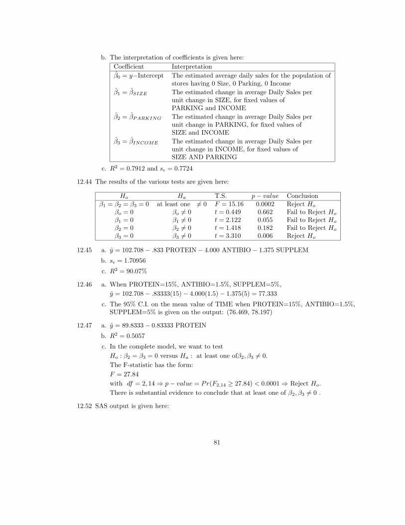
b. The interpretation of coefficients is given here:
Coefficient Interpretation
β0 = y−Intercept The estimated average daily sales for the population ofstores having 0 Size, 0 Parking, 0 Income
β1 = βSIZE The estimated change in average Daily Sales perunit change in SIZE, for fixed values ofPARKING and INCOME
β2 = βPARKING The estimated change in average Daily Sales perunit change in PARKING, for fixed values ofSIZE and INCOME
β3 = βINCOME The estimated change in average Daily Sales perunit change in INCOME, for fixed values ofSIZE AND PARKING
c. R2 = 0.7912 and sε = 0.7724
12.44 The results of the various tests are given here:
Ho Ha T.S. p− value Conclusionβ1 = β2 = β3 = 0 at least one 6= 0 F = 15.16 0.0002 Reject Ho
βo = 0 βo 6= 0 t = 0.449 0.662 Fail to Reject Ho
β1 = 0 β1 6= 0 t = 2.122 0.055 Fail to Reject Ho
β2 = 0 β2 6= 0 t = 1.418 0.182 Fail to Reject Ho
β3 = 0 β3 6= 0 t = 3.310 0.006 Reject Ho
12.45 a. y = 102.708− .833 PROTEIN− 4.000 ANTIBIO− 1.375 SUPPLEM
b. sε = 1.70956
c. R2 = 90.07%
12.46 a. When PROTEIN=15%, ANTIBIO=1.5%, SUPPLEM=5%,
y = 102.708− .83333(15)− 4.000(1.5)− 1.375(5) = 77.333
c. The 95% C.I. on the mean value of TIME when PROTEIN=15%, ANTIBIO=1.5%,SUPPLEM=5% is given on the output: (76.469, 78.197)
12.47 a. y = 89.8333− 0.83333 PROTEIN
b. R2 = 0.5057
c. In the complete model, we want to test
Ho : β2 = β3 = 0 versus Ha : at least one ofβ2, β3 6= 0.
The F-statistic has the form:
F = 27.84
with df = 2, 14⇒ p− value = Pr(F2,14 ≥ 27.84) < 0.0001⇒ Reject Ho.
There is substantial evidence to conclude that at least one of β2, β3 6= 0 .
12.52 SAS output is given here:
81

The REG Procedure
Model: MODEL1
Dependent Variable: y SALARY
Analysis of Variance
Sum of Mean
Source DF Squares Square F Value Pr > F
Model 3 39.31705 13.10568 13.11 <.0001
Error 63 62.95698 0.99932
Corrected Total 66 102.27403
Root MSE 0.99966 R-Square 0.3844
Dependent Mean 29.36418 Adj R-Sq 0.3551
Coeff Var 3.40435
Parameter Estimates
Parameter Standard
Variable Label DF Estimate Error t Value Pr > |t|
Intercept Intercept 1 25.53758 0.64279 39.73 <.0001
x1 NUMEXPL 1 0.00389 0.00172 2.27 0.0269
x2 MARGIN 1 0.09567 0.03652 2.62 0.0110
x3 IPCOST 1 0.21657 0.06917 3.13 0.0026
a. y = 25.53758 + 0.00389 NUMEXPL + 0.09567 MARGIN + 0.21657 IPCOST
b. The F-statistic from the AOV on the output is F = 13.11 with p − value < 0.0001.There is highly significant evidence that the independent variables as a group providesome predictive value for estimating salary.
c. Using the p− values from the output, all three independent variables have relativelysmall p-values (0.0269, 0.0110, 0.0026). Thus, each of the three independent variablesprovide added predictive value to a model containing only two of the independentvariables.
12.53 a. R2 = 0.3844 = 38.44%
b. The SAS output is given here:
82
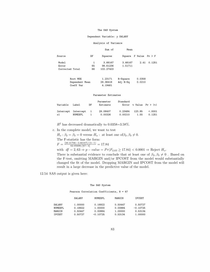
The SAS System
Dependent Variable: y SALARY
Analysis of Variance
Sum of Mean
Source DF Squares Square F Value Pr > F
Model 1 3.66167 3.66167 2.41 0.1251
Error 65 98.61236 1.51711
Corrected Total 66 102.27403
Root MSE 1.23171 R-Square 0.0358
Dependent Mean 29.36418 Adj R-Sq 0.0210
Coeff Var 4.19461
Parameter Estimates
Parameter Standard
Variable Label DF Estimate Error t Value Pr > |t|
Intercept Intercept 1 29.08407 0.23484 123.85 <.0001
x1 NUMEXPL 1 0.00326 0.00210 1.55 0.1251
R2 has decreased dramatically to 0.0358=3.58%.
c. In the complete model, we want to test
Ho : β2 = β3 = 0 versus Ha : at least one ofβ2, β3 6= 0.
The F-statistic has the form:
F = [39.31706−3.66167]/(3−1)62.95698/[67−4] = 17.84
with df = 2, 63⇒ p− value = Pr(F2,63 ≥ 17.84) < 0.0001⇒ Reject Ho.
There is substantial evidence to conclude that at least one of β2, β3 6= 0 . Based onthe F-test, omitting MARGIN and/or IPCOST from the model would substantiallychanged the fit of the model. Dropping MARGIN and IPCOST from the model willresult in a large decrease in the predictive value of the model.
12.54 SAS output is given here:
The SAS System
Pearson Correlation Coefficients, N = 67
SALARY NUMEXPL MARGIN IPCOST
SALARY 1.00000 0.18922 0.50447 0.50727
NUMEXPL 0.18922 1.00000 0.00884 -0.10725
MARGIN 0.50447 0.00884 1.00000 0.53134
IPCOST 0.50727 -0.10725 0.53134 1.00000
83
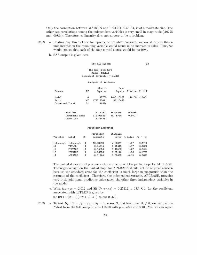
Only the correlation between MARGIN and IPCOST, 0.53134, is of a moderate size. Theother two correlations among the independent variables is very small in magnitude (.10725and .00884). Therefore, collinearity does not appear to be a problem.
12.58 a. Holding any three of the four predictor variables constant, we would expect that aunit increase in the remaining variable would result in an increase in sales. Thus, wewould expect that each of the four partial slopes would be positive.
b. SAS output is given here:
The SAS System 23
The REG Procedure
Model: MODEL1
Dependent Variable: y SALES
Analysis of Variance
Sum of Mean
Source DF Squares Square F Value Pr > F
Model 4 17785 4446.15952 116.68 <.0001
Error 47 1790.93411 38.10498
Corrected Total 51 19576
Root MSE 6.17292 R-Square 0.9085
Dependent Mean 112.96923 Adj R-Sq 0.9007
Coeff Var 5.46425
Parameter Estimates
Parameter Standard
Variable Label DF Estimate Error t Value Pr > |t|
Intercept Intercept 1 -10.08918 7.35341 -1.37 0.1766
x1 TITLES 1 0.44914 0.25412 1.77 0.0836
x2 FOOTAGE 1 0.30836 0.18508 1.67 0.1024
x3 IBMBASE 1 0.06956 0.05110 1.36 0.1799
x4 APLBASE 1 -0.01260 0.08495 -0.15 0.8827
The partial slopes are all positive with the exception of the partial slope for APLBASE.The negative sign on the partial slope for APLBASE should not be of great concernbecause the standard error for the coefficient is much large in magnitude than theestimate of the coefficient. Therefore, the independent variable, APLBASE, providesvery little additional predictive value given the other three independent variables inthe model.
c. With t0.025,47 = 2.012 and SE(βTITLES) = 0.25412, a 95% C.I. for the coefficientassociated with TITLES is given by
0.44914± (2.012)(0.25412)⇒ (−0.062, 0.960).
12.59 a. To test Ho : β1 = β2 = β3 = β4 = 0 versus Ho : at least one βi 6= 0, we can use theF -test from the SAS output: F = 116.68 with p− value < 0.0001. Yes, we can reject
84
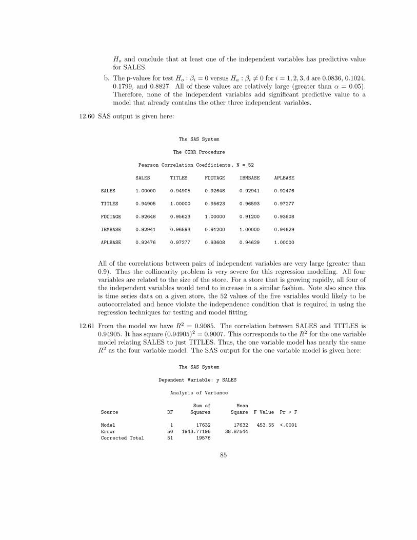
Ho and conclude that at least one of the independent variables has predictive valuefor SALES.
b. The p-values for test Ho : βi = 0 versus Ha : βi 6= 0 for i = 1, 2, 3, 4 are 0.0836, 0.1024,0.1799, and 0.8827. All of these values are relatively large (greater than α = 0.05).Therefore, none of the independent variables add significant predictive value to amodel that already contains the other three independent variables.
12.60 SAS output is given here:
The SAS System
The CORR Procedure
Pearson Correlation Coefficients, N = 52
SALES TITLES FOOTAGE IBMBASE APLBASE
SALES 1.00000 0.94905 0.92648 0.92941 0.92476
TITLES 0.94905 1.00000 0.95623 0.96593 0.97277
FOOTAGE 0.92648 0.95623 1.00000 0.91200 0.93608
IBMBASE 0.92941 0.96593 0.91200 1.00000 0.94629
APLBASE 0.92476 0.97277 0.93608 0.94629 1.00000
All of the correlations between pairs of independent variables are very large (greater than0.9). Thus the collinearity problem is very severe for this regression modelling. All fourvariables are related to the size of the store. For a store that is growing rapidly, all four ofthe independent variables would tend to increase in a similar fashion. Note also since thisis time series data on a given store, the 52 values of the five variables would likely to beautocorrelated and hence violate the independence condition that is required in using theregression techniques for testing and model fitting.
12.61 From the model we have R2 = 0.9085. The correlation between SALES and TITLES is0.94905. It has square (0.94905)2 = 0.9007. This corresponds to the R2 for the one variablemodel relating SALES to just TITLES. Thus, the one variable model has nearly the sameR2 as the four variable model. The SAS output for the one variable model is given here:
The SAS System
Dependent Variable: y SALES
Analysis of Variance
Sum of Mean
Source DF Squares Square F Value Pr > F
Model 1 17632 17632 453.55 <.0001
Error 50 1943.77196 38.87544
Corrected Total 51 19576
85
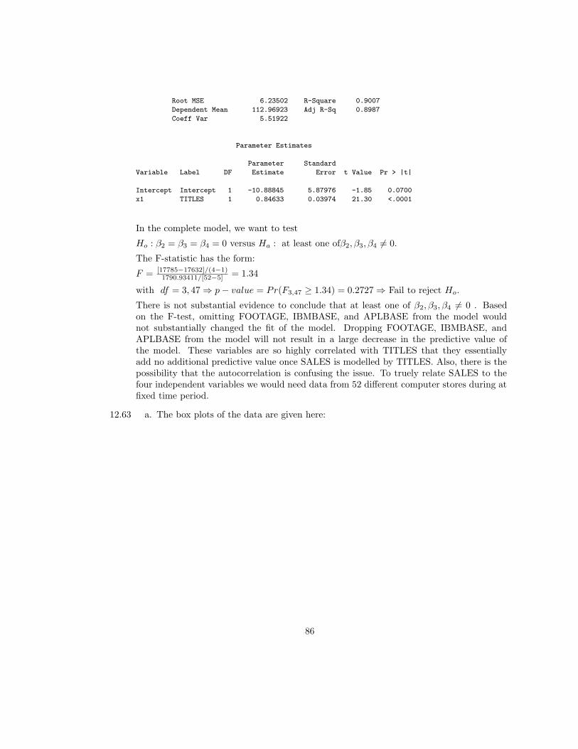
Root MSE 6.23502 R-Square 0.9007
Dependent Mean 112.96923 Adj R-Sq 0.8987
Coeff Var 5.51922
Parameter Estimates
Parameter Standard
Variable Label DF Estimate Error t Value Pr > |t|
Intercept Intercept 1 -10.88845 5.87976 -1.85 0.0700
x1 TITLES 1 0.84633 0.03974 21.30 <.0001
In the complete model, we want to test
Ho : β2 = β3 = β4 = 0 versus Ha : at least one ofβ2, β3, β4 6= 0.
The F-statistic has the form:
F = [17785−17632]/(4−1)1790.93411/[52−5] = 1.34
with df = 3, 47⇒ p− value = Pr(F3,47 ≥ 1.34) = 0.2727⇒ Fail to reject Ho.
There is not substantial evidence to conclude that at least one of β2, β3, β4 6= 0 . Basedon the F-test, omitting FOOTAGE, IBMBASE, and APLBASE from the model wouldnot substantially changed the fit of the model. Dropping FOOTAGE, IBMBASE, andAPLBASE from the model will not result in a large decrease in the predictive value ofthe model. These variables are so highly correlated with TITLES that they essentiallyadd no additional predictive value once SALES is modelled by TITLES. Also, there is thepossibility that the autocorrelation is confusing the issue. To truely relate SALES to thefour independent variables we would need data from 52 different computer stores during atfixed time period.
12.63 a. The box plots of the data are given here:
86
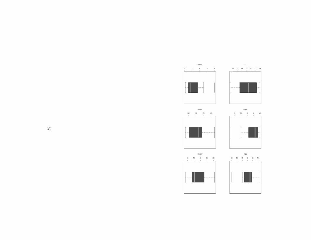
1.2 1.4 1.6 1.8 2.0 2.2 2.4
CI
20 25 30 35 40
PCWP
45 50 55 60 65 70
AGE
0 2 4 6 8
DISDUR
165 170 175 180
HEIGHT
60 70 80 90 100
WEIGHT
87

b. The scatterplots of the data are given here:
•
•
•
•
•
•
•
•
•
•
•
•
AGE
CI
40 50 60 70
1.0
1.4
1.8
2.2
•
•
•
•
•
•
•
•
•
•
•
•
DISEASE DURATION
CI
0 2 4 6 8 10
1.0
1.4
1.8
2.2
•
•
• •
•••
•
•
•
••
AGE
PCW
P
40 50 60 70
1418
2226
3034
38
•
•
••
•• •
•
•
•
••
DISEASE DURATION
PCW
P
0 2 4 6 8 10
1418
2226
3034
38
88
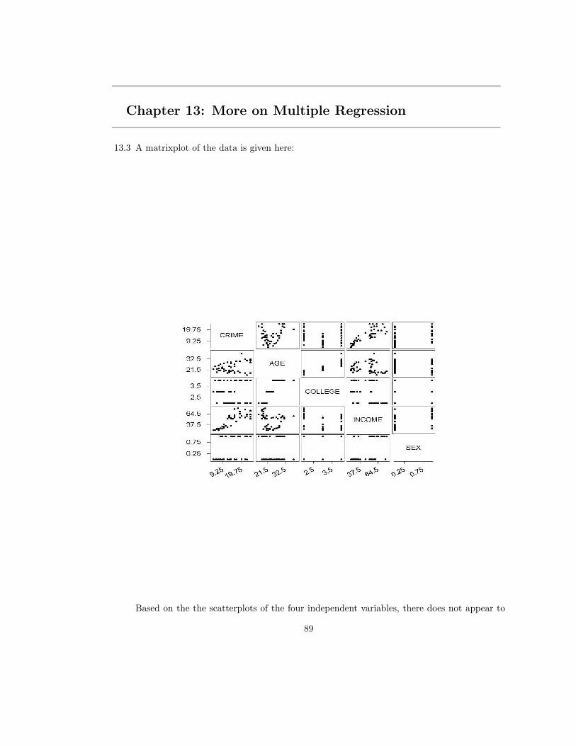
Chapter 13: More on Multiple Regression
13.3 A matrixplot of the data is given here:
Based on the the scatterplots of the four independent variables, there does not appear to
89

be a major problem with collinearity. The variables that would be included in the modelare Age, Income, and Sex. This set of independent variables had a Cp value of 3.007 andR2 = 82.78394%, whereas the model with College, Age, Income, and Sex had a Cp valueof 5.0 and R2 = 82.783774%. Thus, for the model with Age, Income, and Sex, the Cp isnearly equal to p = 3 and the change in R2 by including College is nearly 0.
13.7 The fitted model is
y = 288.062 + 174.815 Log(DOSE)− 0.344 WEIGHT− 0.863 Log(DOSE)*WEIGHT.
13.9 b. An improved approach would be to define three indicator variables:
x1 =
{1 if industry = chemical0 if Otherwise
x2 =
{1 if industry = data processing0 if Otherwise
x3 =
{1 if industry = electronics0 if Otherwise
c. Another indicator variable could be defined to denote whether or not the firm matchesemployee contributions:
x4 =
{1 if firm matches employee contribution0 if Otherwise
13.16 a. The correlation coefficients between the pairs of independent variables are all equal to0. Thus, there is no simple collinearities in the data.
b. Scatterplots of the pairs of independent variable are given here:
90

•
•
•
•
•
•
•
•
•
•
•
•
•
•
•
•
MELT
CH
ILL
500 520 540 560 580
7080
9010
0•
•
•
•
•
•
•
•
•
•
•
•
•
•
•
•
•
•
•
•
•
•
•
•
•
•
•
•
•
•
•
•
MELT
REP
EL
500 520 540 560 580
1020
3040
•
•
•
•
•
•
•
•
•
•
•
•
•
•
•
•
•
•
•
•
•
•
•
•
•
•
•
•
•
•
•
•
CHILL
REP
EL
70 80 90 100
1020
3040
13.17 In each of the plots, there is no obvious pattern of nonlinearity. The residuals appear tobe a random scatter about a horizontal line at height 0.
13.18 a. The R2 has increased from 90.4% to 91.4%. Thus, there was very little change in theR2 value.
b. In the second-order model, we want to test
Ho : β6 = β7 = 0 versus Ha : at least one of β6, β7 6= 0.
The F-statistic has the form:
F = [SSReg.,Complete−SSReg.,Reduced]/(k−g)SSResidual,Complete/[n−(k+1)] = 1.43
with df = 2, 24⇒ p− value = Pr(F2,24 ≥ 1.43) = 0.2590⇒Fail to reject Ho.
13.19 a. The independent variable entered into the model in the following order:
Step 1: REPEL
91
Step 2: KNIFE
Step 3: CHILL
Step 4: MELT
b. The ordering (largest to smallest) of the independent variables based on the magnitudeof their correlation with STIFF
1. REPEL
2. KNIFE
3. CHILL
4. MELT
5. SPEED
13.21 a. Test Ho : β1 = β2 = · · · = β7 = 0 versus Ha : at least one of β′is is not 0.
Test Statistic: F =MS(Regression)
MS(Error)= 1.47 with p-value=0.208.
Fail to reject Ho
b. The p-values for the the t-tests of the seven individual hypotheses: Ha : βi 6= 0are given on the output. Only SIZE with a p-value=0.028 has been shown to havestatistical significance
13.23 a. Nonconstant variance may be present; Weighted least squares or Transformation ofthe dependent variable is needed
d. Potential serial correlation; Need to include terms in the model to account for theserial correlation.
13.24 The Minitab output of regressing y-differences on x-differences is given here:
The orginal data and first differences:
Row y x yd xd
1 11 0.5 * *
2 10 1.0 -1 0.5
3 2 1.2 -8 0.2
4 14 1.4 12 0.2
5 22 1.7 8 0.3
6 10 1.8 -12 0.1
7 20 2.0 10 0.2
8 19 2.3 -1 0.3
9 32 2.5 13 0.2
10 23 2.8 -9 0.3
11 40 3.0 17 0.2
12 37 3.1 -3 0.1
13 30 3.5 -7 0.4
14 43 3.6 13 0.1
15 55 3.8 12 0.2
16 29 4.2 -26 0.4
17 45 4.4 16 0.2
18 60 5.1 15 0.7
19 53 5.2 -7 0.1
20 30 5.4 -23 0.2
21 42 5.5 12 0.1
22 25 6.0 -17 0.5
23 63 6.2 38 0.2
92
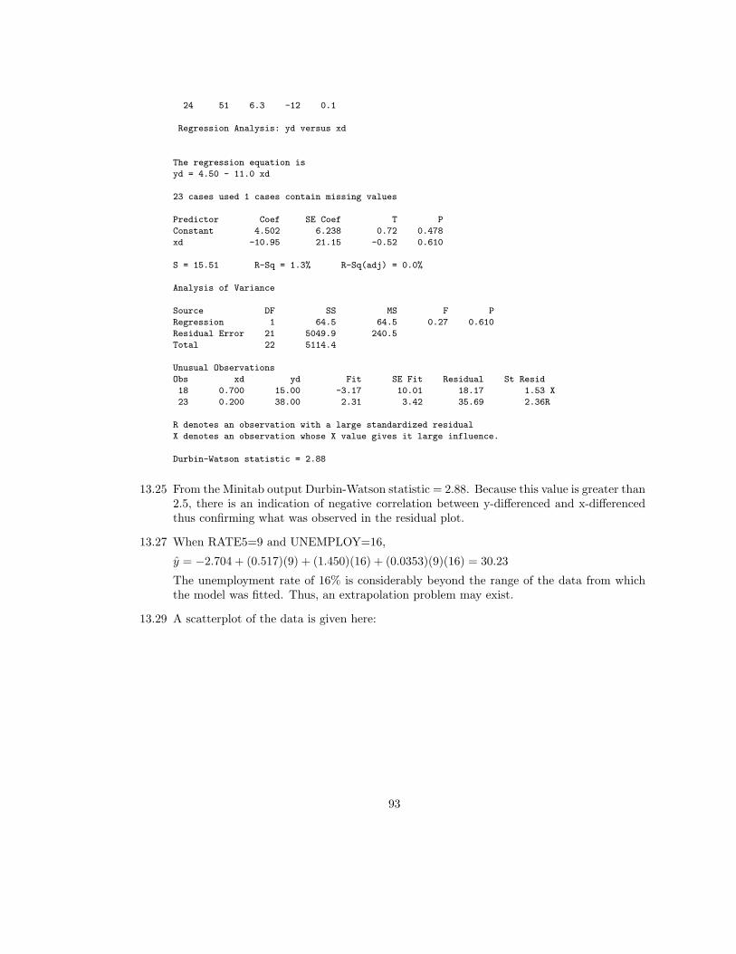
24 51 6.3 -12 0.1
Regression Analysis: yd versus xd
The regression equation is
yd = 4.50 - 11.0 xd
23 cases used 1 cases contain missing values
Predictor Coef SE Coef T P
Constant 4.502 6.238 0.72 0.478
xd -10.95 21.15 -0.52 0.610
S = 15.51 R-Sq = 1.3% R-Sq(adj) = 0.0%
Analysis of Variance
Source DF SS MS F P
Regression 1 64.5 64.5 0.27 0.610
Residual Error 21 5049.9 240.5
Total 22 5114.4
Unusual Observations
Obs xd yd Fit SE Fit Residual St Resid
18 0.700 15.00 -3.17 10.01 18.17 1.53 X
23 0.200 38.00 2.31 3.42 35.69 2.36R
R denotes an observation with a large standardized residual
X denotes an observation whose X value gives it large influence.
Durbin-Watson statistic = 2.88
13.25 From the Minitab output Durbin-Watson statistic = 2.88. Because this value is greater than2.5, there is an indication of negative correlation between y-differenced and x-differencedthus confirming what was observed in the residual plot.
13.27 When RATE5=9 and UNEMPLOY=16,
y = −2.704 + (0.517)(9) + (1.450)(16) + (0.0353)(9)(16) = 30.23
The unemployment rate of 16% is considerably beyond the range of the data from whichthe model was fitted. Thus, an extrapolation problem may exist.
13.29 A scatterplot of the data is given here:
93
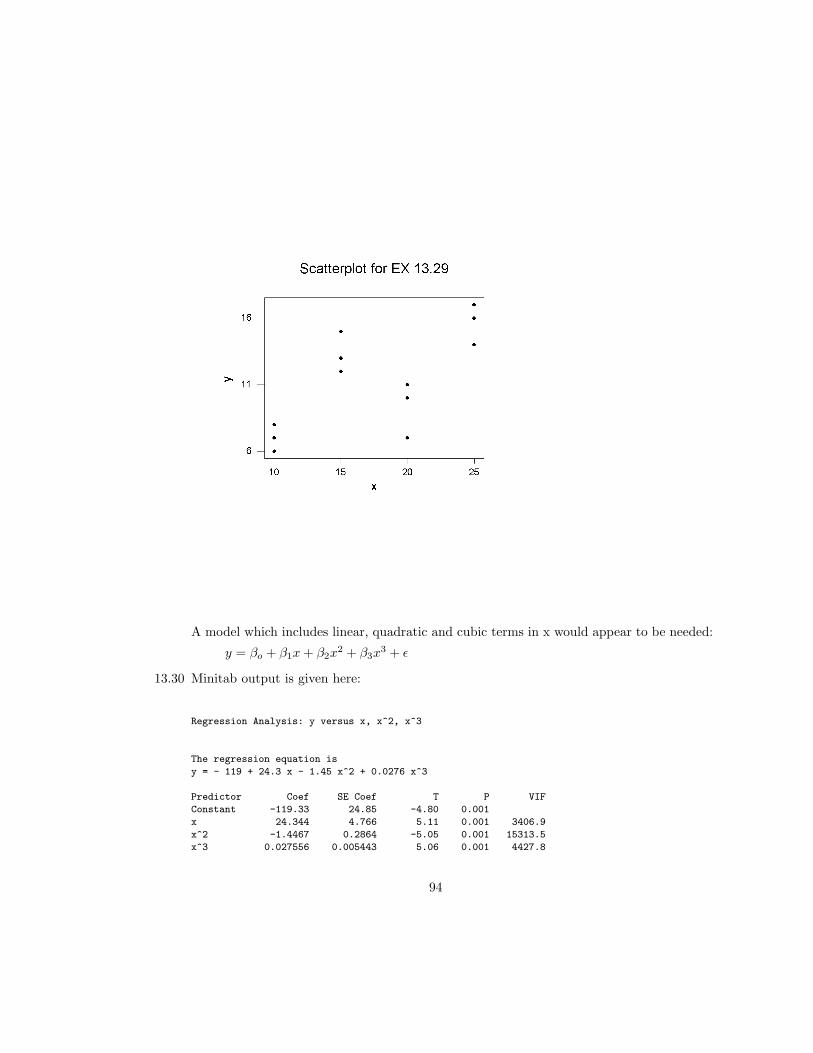
A model which includes linear, quadratic and cubic terms in x would appear to be needed:
y = βo + β1x+ β2x2 + β3x
3 + ε
13.30 Minitab output is given here:
Regression Analysis: y versus x, x^2, x^3
The regression equation is
y = - 119 + 24.3 x - 1.45 x^2 + 0.0276 x^3
Predictor Coef SE Coef T P VIF
Constant -119.33 24.85 -4.80 0.001
x 24.344 4.766 5.11 0.001 3406.9
x^2 -1.4467 0.2864 -5.05 0.001 15313.5
x^3 0.027556 0.005443 5.06 0.001 4427.8
94

S = 1.581 R-Sq = 87.2% R-Sq(adj) = 82.4%
PRESS = 45.0000 R-Sq(pred) = 71.28%
Analysis of Variance
Source DF SS MS F P
Regression 3 136.667 45.556 18.22 0.001
Residual Error 8 20.000 2.500
Total 11 156.667
The number of distinct predictor combinations equals the
number of parameters. No degrees of freedom for lack of fit.
Cannot do pure error test.
Source DF Seq SS
x 1 72.600
x^2 1 0.000
x^3 1 64.067
Durbin-Watson statistic = 2.41
a. The fitted regression equation is
y = −119 + 24.3x− 1.45x2 + 0.0276x3
b. It is not possible to test for lack of fit since the number of distinct values of x equalsthe number of parameters in the model.
13.31 Minitab output is given here:
(EX13-31) Regression Analysis: y versus x, x^2, x^3
The regression equation is
y = - 91.0 + 19.2 x - 1.16 x^2 + 0.0227 x^3
Predictor Coef SE Coef T P VIF
Constant -91.00 35.89 -2.54 0.064
x 19.217 6.820 2.82 0.048 4751.4
x^2 -1.1633 0.4016 -2.90 0.044 19931.4
x^3 0.022667 0.007473 3.03 0.039 5413.7
S = 1.555 R-Sq = 90.7% R-Sq(adj) = 83.7%
PRESS = * R-Sq(pred) = *%
Analysis of Variance
Source DF SS MS F P
Regression 3 94.333 31.444 13.01 0.016
Residual Error 4 9.667 2.417
Total 7 104.000
The number of distinct predictor combinations equals the
number of parameters. No degrees of freedom for lack of fit.
Cannot do pure error test.
95

Source DF Seq SS
x 1 58.329
x^2 1 13.773
x^3 1 22.231
Unusual Observations
Obs x y Fit SE Fit Residual St Resid
3 15.0 12.000 12.000 1.555 0.000 * X
X denotes an observation whose X value gives it large influence.
Durbin-Watson statistic = 2.32
a. The fitted regression equation is
y = −91.0 + 19.2x− 1.16x2 + 0.0227x3
13.33 a. See output on page 787.
b. y = 1.20 + 7.021 LOG(DOSE)
c. See output.
d. The model using LOG(DOSE) appears to provide the better fit:
Larger R2: 92.95% vs 88.15% for Quadratic, 77.30% for Linear
Smaller MS(Error): 4.144 vs 7.548 for Quadratic, 13.345 for Linear
Residual Plots: No apparent pattern for LOG(DOSE) model, whereas both the Quadraticand Linear models have somewhat of a parabolic pattern.
13.37 The Minitab output is given here:
The regression equation is
y = 60.5 - 0.705 x1 + 0.00328 x1^2 + 8.88 x2
Predictor Coef SE Coef T P VIF
Constant 60.477 5.512 10.97 0.000
x1 -0.70507 0.07551 -9.34 0.000 106.5
x1^2 0.0032768 0.0002505 13.08 0.000 106.5
x2 8.875 2.499 3.55 0.001 1.0
S = 1.732 R-Sq = 97.4% R-Sq(adj) = 97.2%
PRESS = 165.551 R-Sq(pred) = 96.70%
Analysis of Variance
Source DF SS MS F P
Regression 3 4877.7 1625.9 542.22 0.000
Residual Error 44 131.9 3.0
Lack of Fit 8 44.2 5.5 2.27 0.044
Pure Error 36 87.7 2.4
Total 47 5009.6
----------------------------------------------------------
Regression Analysis: y versus x1, x1^2, x2, x1*x2, x1^2*x2
The regression equation is
y = 42.3 - 0.421 x1 + 0.00224 x1^2 + 69.5 x2 - 0.949 x1*x2 + 0.00345 x1^2*x2
96
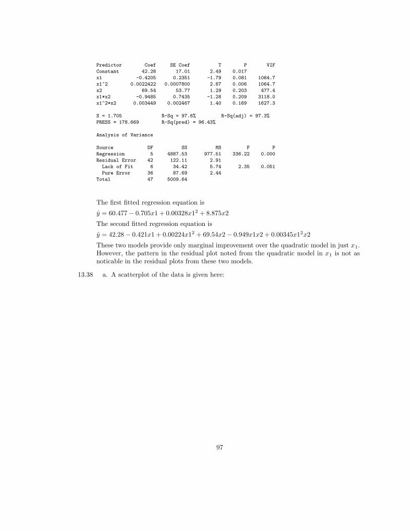
Predictor Coef SE Coef T P VIF
Constant 42.28 17.01 2.49 0.017
x1 -0.4205 0.2351 -1.79 0.081 1064.7
x1^2 0.0022422 0.0007800 2.87 0.006 1064.7
x2 69.54 53.77 1.29 0.203 477.4
x1*x2 -0.9485 0.7435 -1.28 0.209 3118.0
x1^2*x2 0.003449 0.002467 1.40 0.169 1627.3
S = 1.705 R-Sq = 97.6% R-Sq(adj) = 97.3%
PRESS = 178.669 R-Sq(pred) = 96.43%
Analysis of Variance
Source DF SS MS F P
Regression 5 4887.53 977.51 336.22 0.000
Residual Error 42 122.11 2.91
Lack of Fit 6 34.42 5.74 2.35 0.051
Pure Error 36 87.69 2.44
Total 47 5009.64
The first fitted regression equation is
y = 60.477− 0.705x1 + 0.00328x12 + 8.875x2
The second fitted regression equation is
y = 42.28− 0.421x1 + 0.00224x12 + 69.54x2− 0.949x1x2 + 0.00345x12x2
These two models provide only marginal improvement over the quadratic model in just x1.However, the pattern in the residual plot noted from the quadratic model in x1 is not asnoticable in the residual plots from these two models.
13.38 a. A scatterplot of the data is given here:
97
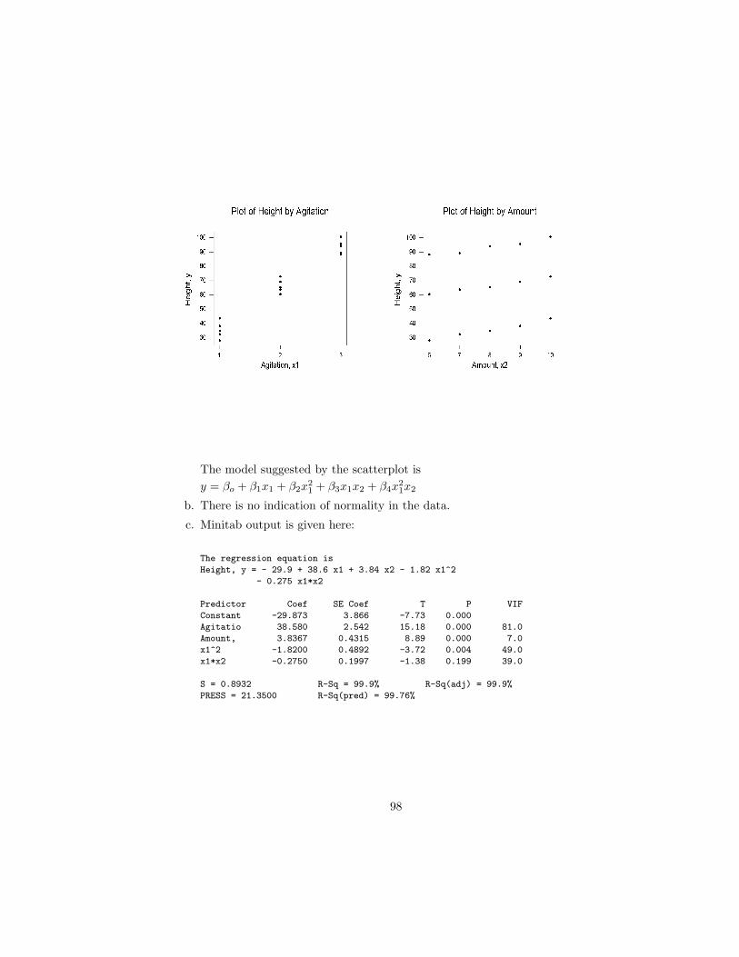
The model suggested by the scatterplot is
y = βo + β1x1 + β2x21 + β3x1x2 + β4x
21x2
b. There is no indication of normality in the data.
c. Minitab output is given here:
The regression equation is
Height, y = - 29.9 + 38.6 x1 + 3.84 x2 - 1.82 x1^2
- 0.275 x1*x2
Predictor Coef SE Coef T P VIF
Constant -29.873 3.866 -7.73 0.000
Agitatio 38.580 2.542 15.18 0.000 81.0
Amount, 3.8367 0.4315 8.89 0.000 7.0
x1^2 -1.8200 0.4892 -3.72 0.004 49.0
x1*x2 -0.2750 0.1997 -1.38 0.199 39.0
S = 0.8932 R-Sq = 99.9% R-Sq(adj) = 99.9%
PRESS = 21.3500 R-Sq(pred) = 99.76%
98
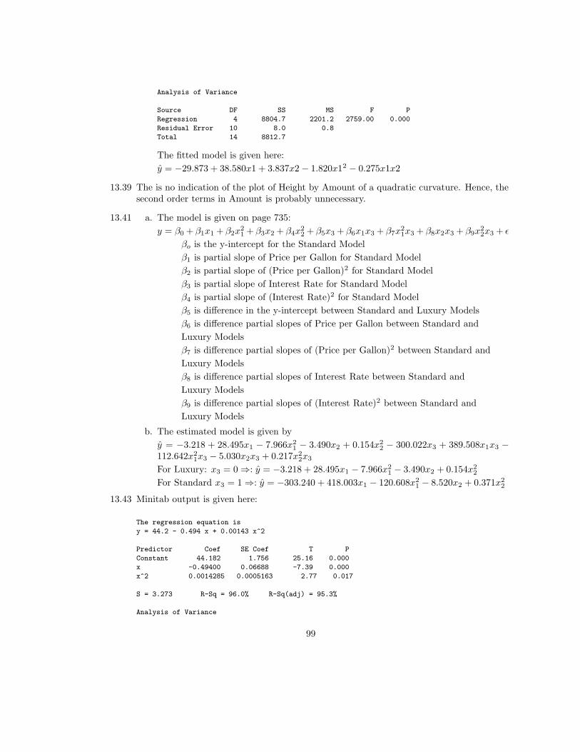
Analysis of Variance
Source DF SS MS F P
Regression 4 8804.7 2201.2 2759.00 0.000
Residual Error 10 8.0 0.8
Total 14 8812.7
The fitted model is given here:
y = −29.873 + 38.580x1 + 3.837x2− 1.820x12 − 0.275x1x2
13.39 The is no indication of the plot of Height by Amount of a quadratic curvature. Hence, thesecond order terms in Amount is probably unnecessary.
13.41 a. The model is given on page 735:
y = β0 + β1x1 + β2x21 + β3x2 + β4x
22 + β5x3 + β6x1x3 + β7x
21x3 + β8x2x3 + β9x
22x3 + ε
βo is the y-intercept for the Standard Model
β1 is partial slope of Price per Gallon for Standard Model
β2 is partial slope of (Price per Gallon)2 for Standard Model
β3 is partial slope of Interest Rate for Standard Model
β4 is partial slope of (Interest Rate)2 for Standard Model
β5 is difference in the y-intercept between Standard and Luxury Models
β6 is difference partial slopes of Price per Gallon between Standard and
Luxury Models
β7 is difference partial slopes of (Price per Gallon)2 between Standard and
Luxury Models
β8 is difference partial slopes of Interest Rate between Standard and
Luxury Models
β9 is difference partial slopes of (Interest Rate)2 between Standard and
Luxury Models
b. The estimated model is given by
y = −3.218 + 28.495x1 − 7.966x21 − 3.490x2 + 0.154x2
2 − 300.022x3 + 389.508x1x3 −112.642x2
1x3 − 5.030x2x3 + 0.217x22x3
For Luxury: x3 = 0⇒: y = −3.218 + 28.495x1 − 7.966x21 − 3.490x2 + 0.154x2
2
For Standard x3 = 1⇒: y = −303.240 + 418.003x1 − 120.608x21 − 8.520x2 + 0.371x2
2
13.43 Minitab output is given here:
The regression equation is
y = 44.2 - 0.494 x + 0.00143 x^2
Predictor Coef SE Coef T P
Constant 44.182 1.756 25.16 0.000
x -0.49400 0.06688 -7.39 0.000
x^2 0.0014285 0.0005163 2.77 0.017
S = 3.273 R-Sq = 96.0% R-Sq(adj) = 95.3%
Analysis of Variance
99
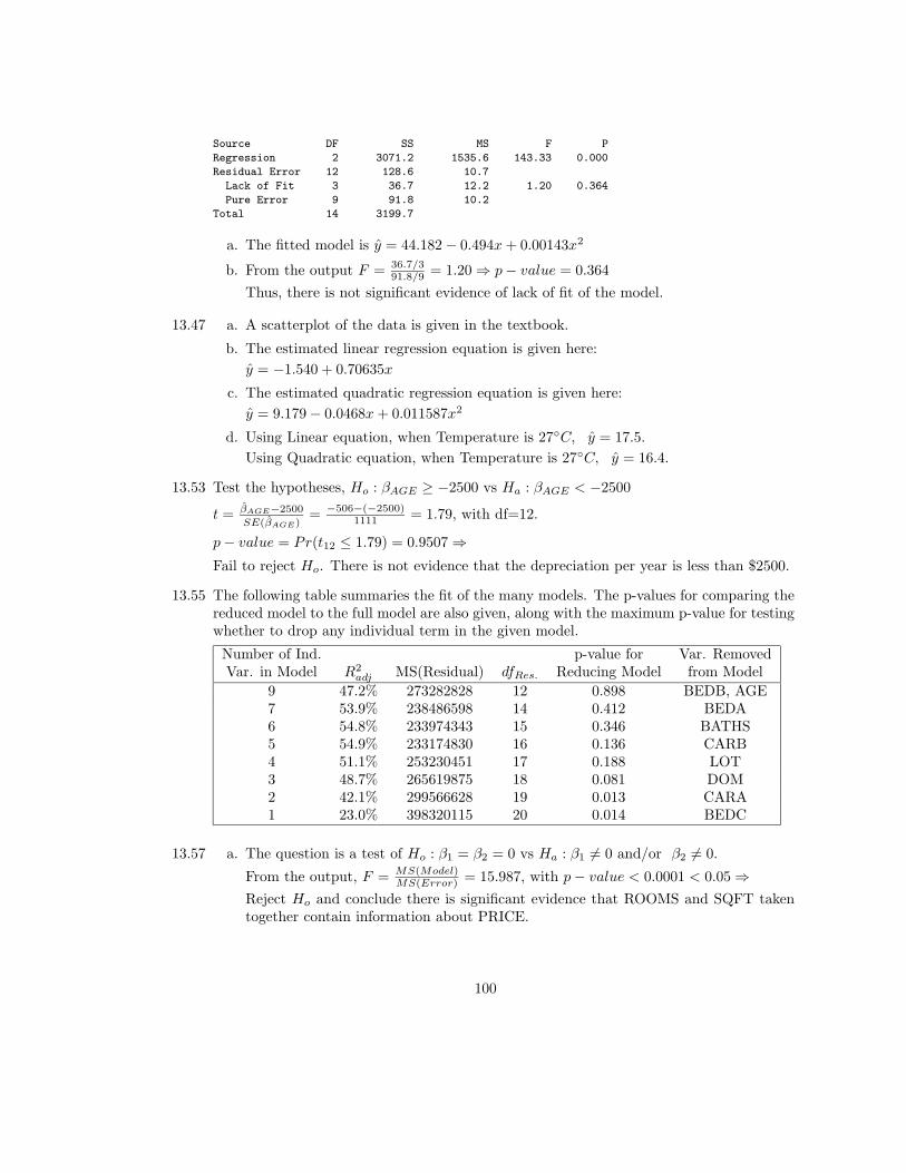
Source DF SS MS F P
Regression 2 3071.2 1535.6 143.33 0.000
Residual Error 12 128.6 10.7
Lack of Fit 3 36.7 12.2 1.20 0.364
Pure Error 9 91.8 10.2
Total 14 3199.7
a. The fitted model is y = 44.182− 0.494x+ 0.00143x2
b. From the output F = 36.7/391.8/9 = 1.20⇒ p− value = 0.364
Thus, there is not significant evidence of lack of fit of the model.
13.47 a. A scatterplot of the data is given in the textbook.
b. The estimated linear regression equation is given here:
y = −1.540 + 0.70635x
c. The estimated quadratic regression equation is given here:
y = 9.179− 0.0468x+ 0.011587x2
d. Using Linear equation, when Temperature is 27◦C, y = 17.5.
Using Quadratic equation, when Temperature is 27◦C, y = 16.4.
13.53 Test the hypotheses, Ho : βAGE ≥ −2500 vs Ha : βAGE < −2500
t = βAGE−2500
SE(βAGE)= −506−(−2500)
1111 = 1.79, with df=12.
p− value = Pr(t12 ≤ 1.79) = 0.9507⇒Fail to reject Ho. There is not evidence that the depreciation per year is less than $2500.
13.55 The following table summaries the fit of the many models. The p-values for comparing thereduced model to the full model are also given, along with the maximum p-value for testingwhether to drop any individual term in the given model.
Number of Ind. p-value for Var. RemovedVar. in Model R2
adj MS(Residual) dfRes. Reducing Model from Model
9 47.2% 273282828 12 0.898 BEDB, AGE7 53.9% 238486598 14 0.412 BEDA6 54.8% 233974343 15 0.346 BATHS5 54.9% 233174830 16 0.136 CARB4 51.1% 253230451 17 0.188 LOT3 48.7% 265619875 18 0.081 DOM2 42.1% 299566628 19 0.013 CARA1 23.0% 398320115 20 0.014 BEDC
13.57 a. The question is a test of Ho : β1 = β2 = 0 vs Ha : β1 6= 0 and/or β2 6= 0.
From the output, F = MS(Model)MS(Error) = 15.987, with p− value < 0.0001 < 0.05⇒
Reject Ho and conclude there is significant evidence that ROOMS and SQFT takentogether contain information about PRICE.
100

b. Test Ho : β1 = 0 vs Ha : β1 6= 0.
t = 0.717 with p− value = 0.4822 > 0.05⇒Fail to reject Ho and conclude there is not significant evidence that the coefficient ofROOMS is different from 0.
c. Test Ho : β2 = 0 vs Ha : β2 6= 0.
t = 0.1.468 with p− value = 0.1585 > 0.05⇒Fail to reject Ho and conclude there is not significant evidence that the coefficient ofSQFT is different from 0.
13.59 The F − test for the overall model is 4.42 with p-value=0.0041.
The indicator variable DV3 measures the difference in risk of infection between hospital inthe South and West holding all other variables constant. The coefficient of DV3 is β7 andwe want to test Ho : β7 ≤ .5% vs Ha : β7 > .5%. The test statistic is
t = β7−0.5
SE(β7)= 0.7024−0.5
0.8896 = 0.23 with df=20
p− value = Pr(t20 > 0.23) = 0.4102⇒Fail to reject Ho
13.61 The table on page 818 provides summary information for a one variable at a time eliminationfrom the full model. The following model is selected based on this information:
y = β0 + β1 STAY + β3 RCR + ε
The R2 for this model is 0.5578 vs 0.6072 for the seven variable model.
The MS(Error) for this model is 28.765 vs 25.546 for the seven variable model.
A test of Ho : Two Variable Model vs Ho : Seven Variable Model is given by testing thefollowing parameters in the seven variable model:
Ho : β2 = β4 = β5 = β6 = β7 = 0 vs Ha : at least one of β2, β4, β5, β6, β7 6= 0
F = (39.49805177−36.27961297)/525.54623394/20 = 0.50 with df = 5, 20⇒
p− value = Pr(F5,20 > 0.50) = 0.7726⇒Fail to reject Ho, there is not significant evidence that any of the five parameters are not0. Thus, there is not significant evidence of a difference between the two-variables andseven-variables models.
Based on the above test, the marginal difference in R2 and MS(Error), the model withfewer variables is the more desirable model.
13.63 a. The model F-test has value 6.52 with p-value=0.0004. Thus, we can reject Ho : β1 =β2 = β3 = β4 = β5 = β6 = 0 and conclude that at least one of β1, β2, β3, β4, β5, β6 6= 0.There is significant evidence that the set of six independent variables does provide anexplaination of the variability in PULSE.
101
Chapter 14: Design Concepts for Experiments and Studies
14.1 a. Water Temperature and Type of Hardener
b. Water temperature: 175◦F and 200◦F
Type of Hardener: H1, H2, H3
c. Manufacuring Plants
d. Plastic Pipe
e. Location on Plastic Pipe
f. 2 Pipes per Treatment
g. None
h. 6 Treatments: (175◦F ,H1),(175◦F ,H2),(175◦F ,H3)
(200◦F ,H1),(200◦F ,H2),(200◦F ,H3)
14.3 a. • Factors: Location in Orchard, Location on Tree, Time of Year
• Factor Levels: Location in Orchard: 8 SectionsTime of Year: Oct., Nov., Dec., Jan., Feb., March, April, MayLocation on Tree: Top, Middle, Bottom
• Blocks: None
• Experimental Units: Locaton on Tree during one of the 8 months
• Measurement Units: Oranges
• Replications: For each section, time of year, location on tree, there is one experi-mental unit. Hence 1 rep.
• Covariates: None
• Treatments: 192 combinations of 8-Sections, 8 Months, 3 Locations on Tree yield(Si,Mj , Lk), for i = 1, · · · , 8; j = 1, . . . , 8; k = 1, . . . , 3
c. • Factors: Type of Treatment
• Factor Levels: T1, T2
• Blocks: Hospitals, Wards
• Experimental Units: Patients
• Measurement Units: Patients
• Replications: 2 Patients per Treatment in each of the Ward/Hospital combinations
• Covariates: None
• Treatments: T1, T2
14.5 The necessary parameters are t = 4, D = 30, α = .05, σ = 12.25⇒φ =
√r(30)2
(2)(4)(12.25)2 = .8658√r.
Determine r so that power is .90. Select values for r compute ν1 = t− 1 = 4− 1 = 3, ν2 =t(r−1) = 4(r−1), and φ = .8658
√r, then use Table 14 with α = .05 and t = 4 to determine
power: it would take 6 reps to obtain a power of at least .90.
102
14.9 a. Bake one cake from each recipe in the oven at the same time. Repeat this procedure rtimes. The baking period is a block with the four treatments (recipes) appearing oncein each block. The four recipes should be randomly assigned to the four positions, onecake per position. Repeat this procedure r times.
b. If position in the oven is important, then Position in the oven is a second blockingfactor along with the baking Period. Thus, we have a latin square design. To haver = 4, we would need to have each recipe appear in each Position exactly once withineach of four baking Periods.
c. We now have an incompleteness in the blocking variable Period since only four of thefive recipes can be observed in each Period. In order to achieve some level of balancein the design, we need to select enough Periods in order that each recipe appearsthe same number of times in each period and the same total number of times in thecomplete experiment.
Chapter 15: Analysis of Variance for Standard Designs
15.1 a. The F-test from the ANOVA table tests 2-sided alternatives:
Test Ho : µAttend = µDidNot vs Ho : µAttend 6= µDidNot
The ANOVA table is given here:
Source DF SS MS F p-valuePair 5 1319.42 263.88
Treatment 1 420.08 420.08 71.40 0.0004Error 5 29.42 5.88Total 11 1768.92
Reject Ho
b. RE(RCB,CR)=20.94
15.2 The F-test from the ANOVA table tests 2-sided alternatives
Ho : µAttend = µDidNot vs Ho : µAttend 6= µDidNot.
The paired t-test can test one-sided alternatives:
Ho : µAttend ≤ µDidNot vs Ho : µAttend ≥ µDidNott = 8.45
p− value = Pr(t5 ≥ 8.45) = 0.0002⇒Yes
15.5 a. yij = µ+ αi + βj + εij ; i = 1, 2, 3, j = 1, 2, 3, 4, 5, 6, 7
yij is score on test of jth subject hearing the ith music type
αi is the ith music type effect
103

βj is the jth subject effect
µ = 21.33, α1 = −0.47, α2 = −1.19, α3 = 1.67
β1 = 0, β2 = −3, β3 = 3.33, β4 = −1.33, β5 = 1, β6 = 3.67, β7 = −3.67
b. F = 6.54 with df=2,12.
Therefore, p− value = Pr(F2,12 ≥ 6.54) = 0.0120⇒ Reject Ho : µ1 = µ2 = µ3.
c. An interaction plot of the data is given here:
N
N
N
N
N
N
N
H
H
H
H
H
H
H
C
C
C
C
C
C
C
Interaction Plots
Subject
Test
Sco
res
1 2 3 4 5 6 7
1618
2022
2426
2830
32
N No MusicH Hard RockC Classical
Based on the interaction plot, the additive model may be inappropriate because thereis some crossing of the three lines.
d. t = 3, b = 7⇒ RE(RCB,CR) = 3.86⇒
15.9 a. yij = µ+ αk + βi + γj + εij ; i, j, k = 1, 2, 3, 4;
where yij is the dry weight of a watermellon plant grown in Row i and Column j.
αk is the effect of the kth Treatment on dry weight
βi is the effect of the ith Row on dry weight
γj is the effect of the jth Column on dry weight
b. The overall mean is Y .. = 1.5425
The parameter estimates are given here:
µ = 1.5425, β1 = −.0125, β2 = .005, β3 = 0.0025, β4 = .005
γ1 = .02, γ2 = .0325 γ3 = −.0375, α4 = −.015
α1 = .195, α2 = .1425 α3 = −.12, α4 = −.2175
104

F = 1280.4 with df = 3, 6⇒ p− value < 0.0001
Reject Ho : µ1 = µ2 − µ3 = µ4
15.12 a. Ten reps of a completely randomized design with a 3x2 factorial treatment structure.
b. yijk = µ+ αi + βj + αβij + εijk; i = 1, 2, 3; j = 1, 2; k = 1, · · · , 10;
where yijk is the attention span of the kth child of Age i viewing Product j.
αi is the effect of the ith Age on attention span
βj is the effect of the jth Product on attention span
αβij is the interaction effect of the ith Age and jth Product on attention span
c. µ = 27.27, α1 = −4.27, α2 = −2.22, α3 = 6.48
β1 = −5.8, β2 = 5.8
αβ11 = 5.7, αβ21 = .35, αβ31 = −6.05
αβ12 = −5.7, αβ22 = −.35, αβ32 = 6.05
d. The ANOVA table is given here:
Source DF SS MS F p-valueAge 2 1303.0 651.5 4.43 0.017
Product 1 2018.4 2018.4 13.72 0.001Interaction 2 1384.3 692.1 4.70 0.013
Error 54 7944 147.1Total 59 12649.7
15.13 a. A profile plot of the data is given here:
1
1
1
2
2
2
Interaction Plots
AGE
Mea
n At
tent
ion
Span
1 2 3
2025
3035
4045
50
1 - Cereals2 - Games
105
The profile plot indicates an increasing effect of Product Type as Age increases.
15.15 AOV table:
Source DF SS MS F p-valueTreatment 14 SST MSTFactor A 2 SSA MSA MSA/MSEFactor B 4 SSB MSB MSB/MSEInteraction 8 SSAB MSAB MSAB/MSEBlocks 2 SSBL MSBLError 28 SSE MSETotal 44 SSTOT
15.21 a. The design is a completely randomized 4x4 factorial experiment with Factor A - CuRate and Factor B - Mn Rate. There are two replications of the 16 treatments.
b. A model for this experiment is given here:
yijk = µ+ αi + βj + αβij + εijk; i = 1, 2, 3, 4; j = 1, 2, 3, 4; k = 1, 2;
where yijk is the soybean yield of the kth plot using the ith Cu Rate and jth MnRate.
αi is the effect of the ith Cu Rate on yield
βj is the effect of the jth Mn Rate on yield
αβij is the interaction effect of the ith Cu Rate and jth Mn Rate on soybean yield.
c. A profile plot of the data is given here:
106
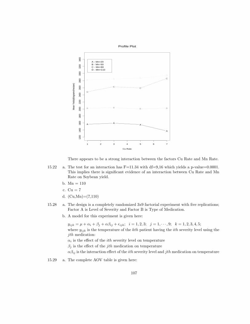
AA
A
A
B B B B
C
CC
CD D D
D
Profile Plot
Cu Rate
Mea
n Yi
elds
(kilo
gram
s/he
ctar
e)
1 2 3 4 5 6 7
1200
1400
1600
1800
2000
2200
2400
2600
2800
3000
3200
3400
A - Mn=20B - Mn=50C - Mn=80D - Mn=110
There appears to be a strong interaction between the factors Cu Rate and Mn Rate.
15.22 a. The test for an interaction has F=11.34 with df=9,16 which yields a p-value=0.0001.This implies there is significant evidence of an interaction between Cu Rate and MnRate on Soybean yield.
b. Mn = 110
c. Cu = 7
d. (Cu,Mn)=(7,110)
15.28 a. The design is a completely randomized 3x9 factorial experiment with five replications;Factor A is Level of Severity and Factor B is Type of Medication.
b. A model for this experiment is given here:
yijk = µ+ αi + βj + αβij + εijk; i = 1, 2, 3; j = 1, · · · , 9; k = 1, 2, 3, 4, 5;
where yijk is the temperature of the kth patient having the ith severity level using thejth medication:
αi is the effect of the ith severity level on temperature
βj is the effect of the jth medication on temperature
αβij is the interaction effect of the ith severity level and jth medication on temperature
15.29 a. The complete AOV table is given here:
107
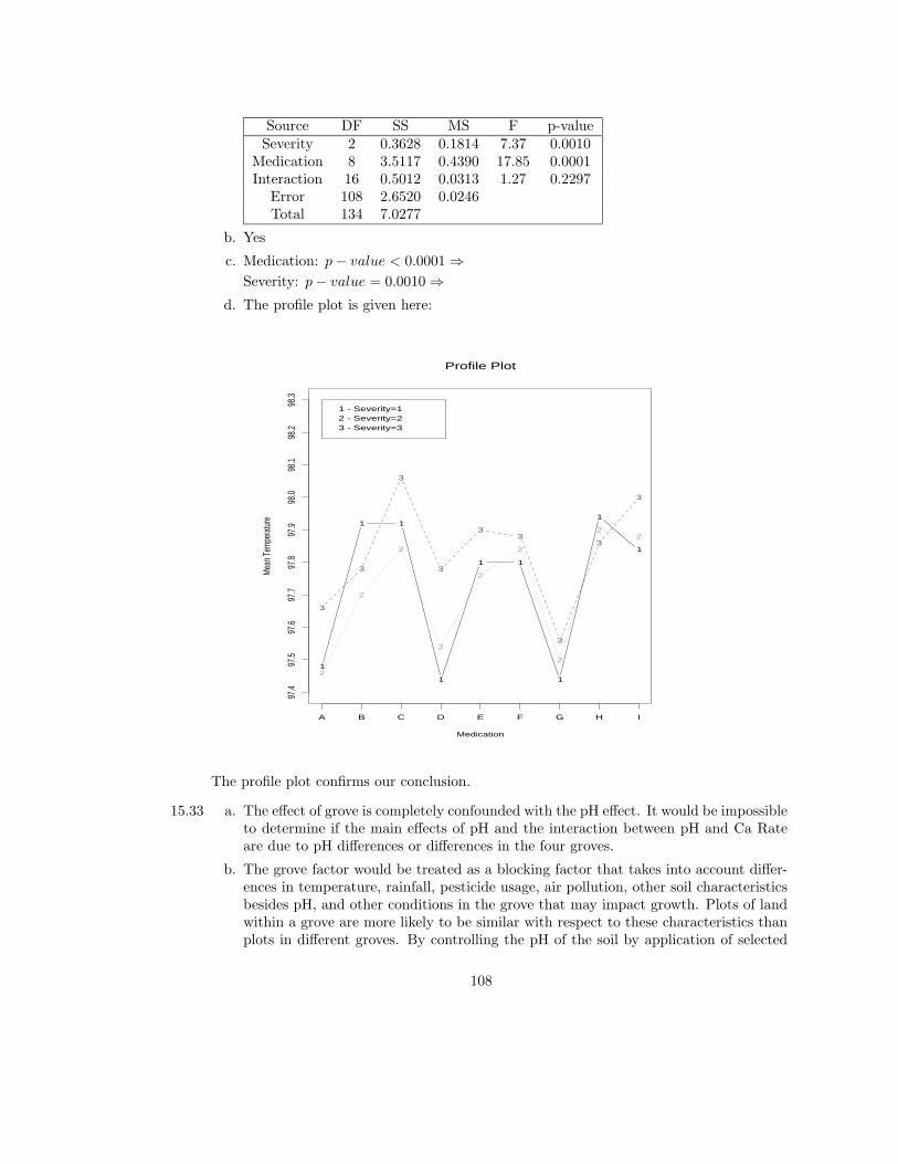
Source DF SS MS F p-valueSeverity 2 0.3628 0.1814 7.37 0.0010
Medication 8 3.5117 0.4390 17.85 0.0001Interaction 16 0.5012 0.0313 1.27 0.2297
Error 108 2.6520 0.0246Total 134 7.0277
b. Yes
c. Medication: p− value < 0.0001⇒Severity: p− value = 0.0010⇒
d. The profile plot is given here:
1
1 1
1
1 1
1
1
1
2
2
2
2
2
2
2
22
3
3
3
3
33
3
3
3
Profile Plot
Medication
Mea
n Te
mpe
ratu
re
97.4
97.5
97.6
97.7
97.8
97.9
98.0
98.1
98.2
98.3
1 - Severity=12 - Severity=23 - Severity=3
A B C D E F G H I
The profile plot confirms our conclusion.
15.33 a. The effect of grove is completely confounded with the pH effect. It would be impossibleto determine if the main effects of pH and the interaction between pH and Ca Rateare due to pH differences or differences in the four groves.
b. The grove factor would be treated as a blocking factor that takes into account differ-ences in temperature, rainfall, pesticide usage, air pollution, other soil characteristicsbesides pH, and other conditions in the grove that may impact growth. Plots of landwithin a grove are more likely to be similar with respect to these characteristics thanplots in different groves. By controlling the pH of the soil by application of selected
108
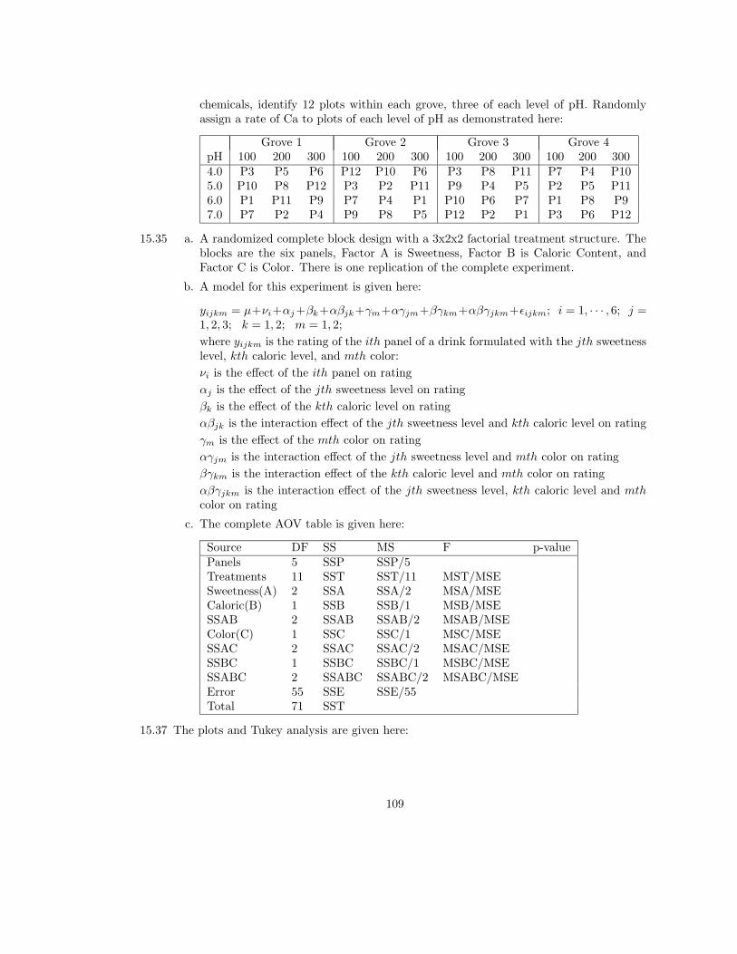
chemicals, identify 12 plots within each grove, three of each level of pH. Randomlyassign a rate of Ca to plots of each level of pH as demonstrated here:
Grove 1 Grove 2 Grove 3 Grove 4pH 100 200 300 100 200 300 100 200 300 100 200 3004.0 P3 P5 P6 P12 P10 P6 P3 P8 P11 P7 P4 P105.0 P10 P8 P12 P3 P2 P11 P9 P4 P5 P2 P5 P116.0 P1 P11 P9 P7 P4 P1 P10 P6 P7 P1 P8 P97.0 P7 P2 P4 P9 P8 P5 P12 P2 P1 P3 P6 P12
15.35 a. A randomized complete block design with a 3x2x2 factorial treatment structure. Theblocks are the six panels, Factor A is Sweetness, Factor B is Caloric Content, andFactor C is Color. There is one replication of the complete experiment.
b. A model for this experiment is given here:
yijkm = µ+νi+αj+βk+αβjk+γm+αγjm+βγkm+αβγjkm+εijkm; i = 1, · · · , 6; j =1, 2, 3; k = 1, 2; m = 1, 2;
where yijkm is the rating of the ith panel of a drink formulated with the jth sweetnesslevel, kth caloric level, and mth color:
νi is the effect of the ith panel on rating
αj is the effect of the jth sweetness level on rating
βk is the effect of the kth caloric level on rating
αβjk is the interaction effect of the jth sweetness level and kth caloric level on rating
γm is the effect of the mth color on rating
αγjm is the interaction effect of the jth sweetness level and mth color on rating
βγkm is the interaction effect of the kth caloric level and mth color on rating
αβγjkm is the interaction effect of the jth sweetness level, kth caloric level and mthcolor on rating
c. The complete AOV table is given here:
Source DF SS MS F p-valuePanels 5 SSP SSP/5Treatments 11 SST SST/11 MST/MSESweetness(A) 2 SSA SSA/2 MSA/MSECaloric(B) 1 SSB SSB/1 MSB/MSESSAB 2 SSAB SSAB/2 MSAB/MSEColor(C) 1 SSC SSC/1 MSC/MSESSAC 2 SSAC SSAC/2 MSAC/MSESSBC 1 SSBC SSBC/1 MSBC/MSESSABC 2 SSABC SSABC/2 MSABC/MSEError 55 SSE SSE/55Total 71 SST
15.37 The plots and Tukey analysis are given here:
109

1
1
1
2
2
2
Profile Plot Sweetness by Caloric Level
Sweetness Level
Mea
n Ra
ting
1 2 3
3540
4550
5560
6570
75
1 - Caloric Content 12 - Caloric Content 2
1
1
1
2
2
2
Profile Plot Sweetness by Color
Sweetness Level
Mea
n Ra
ting
1 2 3
3035
4045
5055
6065
1 - Color 12 - Color 2
Using Tukey’sW -procedure with α = 0.05, s2ε = MSE = 27.48, qα(t, dferror) = q.05(3, 60) =
3.40⇒W = (3.40)
√27.48
12 = 5.15⇒
Sweetness LevelCaloric Content 1 2 3
1 Mean 57.00 65.75 43.55Grouping b c a
2 Mean 41.30 49.85 34.75Grouping b c a
Sweetness LevelColor 1 2 3
1 Mean 51.00 58.20 45.65Grouping b c a
2 Mean 47.30 57.40 32.65Grouping b c a
From the above table we observe that the interactions although significant were all orderly.
15.40 a. The experiment is run as three reps of a completely randomized design with a 2x4factorial treatment structure. A model for the experiment is given here:
yijk = µ+ αi + βj + αβij + εijk; i = 1, 2, 3, 4; j = 1, 2; k = 1, 2, 3;
where yijk is the amount of active ingredient (or pH) of the kth vial having the ithstorage time in laboratory jth:
αi is the effect of the ith storage time on amount of active ingredient (or pH)
βj is the effect of the jth laboratory on amount of active ingredient (or pH)
αβij is the interaction effect of the ith storage time and jth laboratory on amount ofactive ingredient (or pH)
110
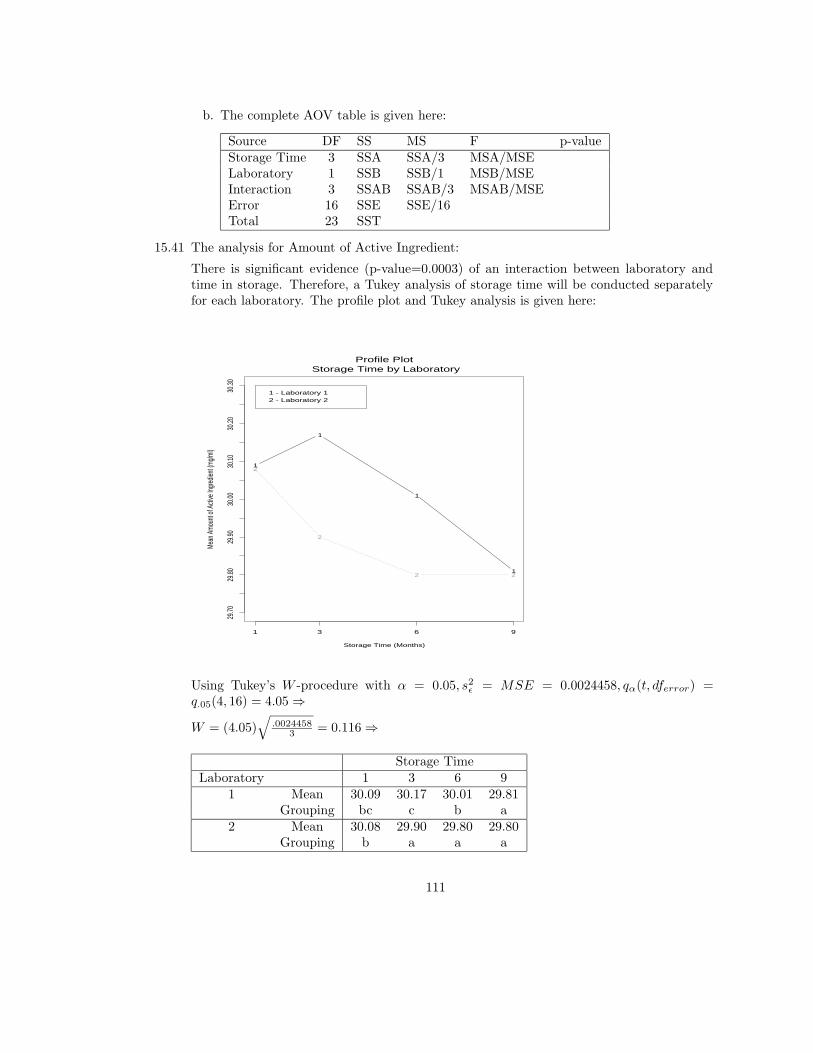
b. The complete AOV table is given here:
Source DF SS MS F p-valueStorage Time 3 SSA SSA/3 MSA/MSELaboratory 1 SSB SSB/1 MSB/MSEInteraction 3 SSAB SSAB/3 MSAB/MSEError 16 SSE SSE/16Total 23 SST
15.41 The analysis for Amount of Active Ingredient:
There is significant evidence (p-value=0.0003) of an interaction between laboratory andtime in storage. Therefore, a Tukey analysis of storage time will be conducted separatelyfor each laboratory. The profile plot and Tukey analysis is given here:
1
1
1
1
2
2
2 2
Profile Plot Storage Time by Laboratory
Storage Time (Months)
Mean
Amo
unt o
f Acti
ve In
gred
ient (
mg/m
l)
29.70
29.80
29.90
30.00
30.10
30.20
30.30
1 - Laboratory 12 - Laboratory 2
1 3 6 9
Using Tukey’s W -procedure with α = 0.05, s2ε = MSE = 0.0024458, qα(t, dferror) =
q.05(4, 16) = 4.05⇒
W = (4.05)√
.00244583 = 0.116⇒
Storage TimeLaboratory 1 3 6 9
1 Mean 30.09 30.17 30.01 29.81Grouping bc c b a
2 Mean 30.08 29.90 29.80 29.80Grouping b a a a
111

15.42 a. With respect to Amount of Active Ingredient:
The profile plots for the two-way interactions are given here:
1
1
1
1
2
2
22
Profile Plot Storage Time by Laboratory
Storage Time (Months)
Me
an
Am
ou
nt
of
Act
ive
In
gre
die
nt
(mg
/ml)
29
.70
29
.80
29
.90
30
.00
30
.10
30
.20
30
.30
1 - Laboratory 12 - Laboratory 2
1 3 6 9
3
3
3
3
4
4
4
4
Profile Plot Storage Time by Temperature
Storage Time (Months)
Me
an
Am
ou
nt
of
Act
ive
In
gre
die
nt
(mg
/ml)
29
.70
29
.80
29
.90
30
.00
30
.10
30
.20
30
.30
3 - Temp=30 C4 - Temp=40 C
1 3 6 9
1
1
2
2
Profile Plot Laboratory by Temperature
Temperature (C)
Me
an
Am
ou
nt
of
Act
ive
In
gre
die
nt
(mg
/ml)
29
.80
29
.84
29
.88
29
.92
29
.96
30
.00
30
.04
30
.08 1 - Laboratory 1
2 - Laboratory 2
30 40
The Time*Lab*Temp interaction (p-value=.6914), Lab*Temp interaction
(p-value=.3519), and Time*Temp interaction (p-value=.2817) were not significant.However, there was significant evidence (p-value=.0192) of a difference in the meansfor Amount of Active Ingredient at the two temperatures. There is a strong interactionbetween Time and Lab (p-value<.0001).
15.43 a. The test for an interaction yields p-value=0.0255. The following profile plot displaysthe interaction:
112
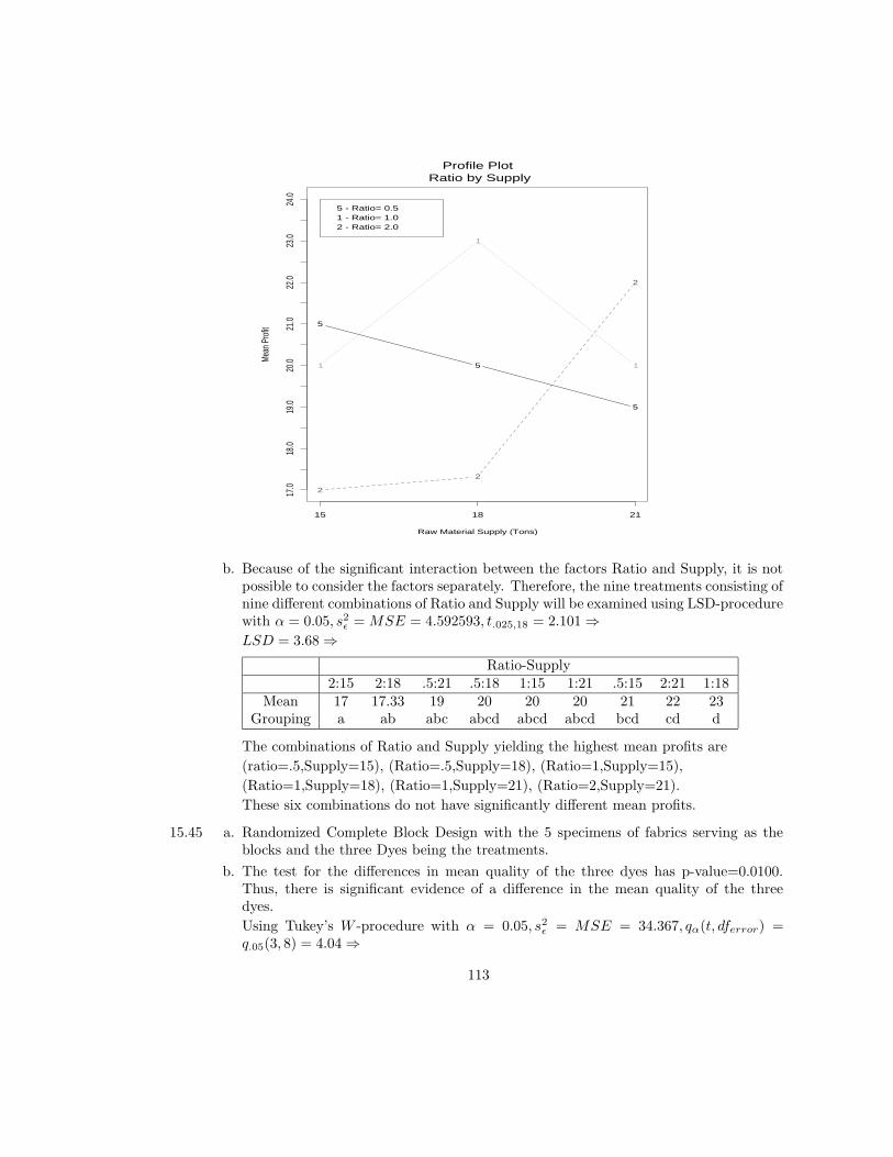
5
5
5
1
1
1
2
2
2
Profile Plot Ratio by Supply
Raw Material Supply (Tons)
Mea
n Pr
ofit
17.0
18.0
19.0
20.0
21.0
22.0
23.0
24.0
5 - Ratio= 0.51 - Ratio= 1.02 - Ratio= 2.0
15 18 21
b. Because of the significant interaction between the factors Ratio and Supply, it is notpossible to consider the factors separately. Therefore, the nine treatments consisting ofnine different combinations of Ratio and Supply will be examined using LSD-procedurewith α = 0.05, s2
ε = MSE = 4.592593, t.025,18 = 2.101⇒LSD = 3.68⇒
Ratio-Supply2:15 2:18 .5:21 .5:18 1:15 1:21 .5:15 2:21 1:18
Mean 17 17.33 19 20 20 20 21 22 23Grouping a ab abc abcd abcd abcd bcd cd d
The combinations of Ratio and Supply yielding the highest mean profits are
(ratio=.5,Supply=15), (Ratio=.5,Supply=18), (Ratio=1,Supply=15),
(Ratio=1,Supply=18), (Ratio=1,Supply=21), (Ratio=2,Supply=21).
These six combinations do not have significantly different mean profits.
15.45 a. Randomized Complete Block Design with the 5 specimens of fabrics serving as theblocks and the three Dyes being the treatments.
b. The test for the differences in mean quality of the three dyes has p-value=0.0100.Thus, there is significant evidence of a difference in the mean quality of the threedyes.
Using Tukey’s W -procedure with α = 0.05, s2ε = MSE = 34.367, qα(t, dferror) =
q.05(3, 8) = 4.04⇒
113
W = (4.04)√
34.3675 = 10.59⇒
DyeA B C
Mean 77.40 84.60 92.80Grouping a ab b
c. RE(RCB,CR) = 0.91⇒
15.47 a. Latin Square Design with blocking variables Farm and Fertility. The treatment is thefive types of fertilizers.
b. There is significant evidence (p− value < 0.0001) the mean yields are different for thefive fertilizers.
15.48 Using Tukey’sW -procedure with α = 0.05, s2ε = MSE = .3886, qα(t, dferror) = q.05(5, 12) =
4.52⇒W = (4.52)
√.3886
5 = 1.26⇒
FertilizerA B C D E
Mean 5.32 6.56 7.64 7.88 8.24Grouping a ab bc c c
The following pairs of fertilizers have significantly different mean yields:
(A,C), (A,D), (A,E), (B,D), (B,E)
114
Chapter 16: The Analysis of Covariance
16.1 yi = βo + β1x1i + β2x2i + β3x3i + β4x4i + β5x5i
+β6x1ix2i + β7x1ix3i + β8x1ix4i + β9x1ix5i + εi for i = 1, · · · , 30
x1 = Covariate
x2 =
{1 if Treatment 2 is applied0 if Otherwise
x3 =
{1 if Treatment 3 is applied0 if Otherwise
x4 =
{1 if Treatment 4 is applied0 if Otherwise
x5 =
{1 if Treatment 5 is applied0 if Otherwise
The coefficients are identified through the mean response under each treatment:
Treatment Mean Response1 βo + β1x1
2 (βo + β2) + (β1 + β6)x1
3 (βo + β3) + (β1 + β7)x1
4 (βo + β4) + (β1 + β8)x1
5 (βo + β5) + (β1 + β9)x1
16.3 Parallelism results from the five lines having the same slope, i.e., the correct model followsthe null hypothesis:
Ho : β6 = β7 = β8 = β9 = 0.
A test of Ho versus the alternative
Ha : At least one of β6, β7, β8, β9 is not zero
consists of fitting two models:
Model 1 (Assumes Ha is true): yi = βo+β1x1i+β2x2i+β3x3i+β4x4i+β5x5i+β6x1ix2i+β7x1ix3i + β8x1ix4i + β9x1ix5i + ε
Model 2 (Assumes Ho is true): yi = βo + β1x1i + β2x2i + β3x3i + β4x4i + β5x5i + ε
Let MSdrop = (SSE2 − SSE1)/(dfE2 − dfE1) = (SSE2 − SSE1)/((30− 6)− (30− 10))
The test statistic is F =MSdropMSE1
, with df1 = (30− 6)− (30− 10) = 4, df2 = 30− 10 = 20.
16.5 A scatterplot of the data is given here:
115
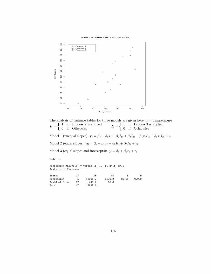
1
1
1
1
1
1
2
2
2
2
2
2
3
3
3
3
3
3
Film Thickness vs Temperature
Temperature
Film
Thick
ness
10 15 20 25 30 35 40
6070
8090
100
110
120
130
140
150
160
170
1 - Process 12 - Process 23 - Process 3
The analysis of variance tables for three models are given here: x = Temperature
I1 =
{1 if Process 2 is applied0 if Otherwise
I2 =
{1 if Process 3 is applied0 if Otherwise
Model 1 (unequal slopes): yi = βo + β1xi + β2I1i + β3I2i + β4xiI1i + β5xiI2i + εi
Model 2 (equal slopes): yi = βo + β1xi + β2I1i + β3I2i + εi
Model 3 (equal slopes and intercepts): yi = βo + β1xi + εi
Model 1:
Regression Analysis: y versus I1, I2, x, x*I1, x*I2
Analysis of Variance
Source DF SS MS F P
Regression 5 16396.2 3279.2 89.15 0.000
Residual Error 12 441.4 36.8
Total 17 16837.6
116
Model 2:
Regression Analysis: y versus I1, I2, x
The regression equation is
y = 26.081 + 19.655 I1 - 21.176 I2 + 3.1879 x
Analysis of Variance
Source DF SS MS F P
Regression 3 16092.2 5364.1 100.74 0.000
Residual Error 14 745.4 53.2
Total 17 16837.6
----------------------------------------------------------------
Model 3:
Regression Analysis: y versus x
The regression equation is
y = - 1.71 + 4.1529 x
Analysis of Variance
Source DF SS MS F P
Regression 1 11721 11721 36.65 0.000
Residual Error 16 5116 320
Total 17 16838
The test of equal slopes:
MSdrop = 152⇒ F = 4.13 with df = 2, 12⇒p− value = Pr(F2,12 ≥ 4.13) = 0.0432 > 0.01⇒Fail to reject Ho
The test of difference in mean film thickness for the three processes:
MSdrop = 2185.3⇒ F = 41.08 with df = 2, 14⇒p− value = 0.0001 < 0.01⇒Reject Ho
16.6 yi = βo + β1x1i + β2x2i + β3x3i + β4x4i + β5x1ix2i + β6x1ix3i + β7x1ix4i
+β8x5i + β9x6i + β10x7i + β11x8i + β12x9i + β13x10i + εi for i = 1, · · · , 16
x1 = Covariate
x2 =
{1 if Treatment 2 is applied0 if Otherwise
x3 =
{1 if Treatment 3 is applied0 if Otherwise
x4 =
{1 if Treatment 4 is applied0 if Otherwise
x5 =
{1 if Observation in Row 20 if Otherwise
x6 =
{1 if Observation in Row 30 if Otherwise
x7 =
{1 if Observation in Row 40 if Otherwise
117
x8 =
{1 if Observation in Column 20 if Otherwise
x9 =
{1 if Observation in Column 30 if Otherwise
x10 =
{1 if Observation in Column 40 if Otherwise
16.7 a. Obtain SSE1 from the model in Exercise 16.6. Obtain SSE2 from the model assumingthe lines are parallel: yi = βo+β1x1i+β2x2i+β3x3i+β4x4i+β8x5i+β9x6i+β10x7i+β11x8i + β12x9i + β13x10i + εi
MSdrop = (SSE2 − SSE1)/(5− 2)
F =MSdropMSE1
, with df=3,2
b. Obtain SSE1 from the model assuming the lines are parallel:
yi = βo + β1x1i + β2x2i + β3x3i + β4x4i + β8x5i + β9x6i + β10x7i + β11x8i + β12x9i +β13x10i + εi
Obtain SSE2 from the model assuming no treatment difference:
yi = βo + β1x1i + β8x5i + β9x6i + β10x7i + β11x8i + β12x9i + β13x10i + εi
MSdrop = (SSE2 − SSE1)/(5− 2)
F =MSdropMSE1
, with df=3,5
16.9 a. Randomized complete block design with the three antidepressants as treatments, age-sex combinations as six blocks, and the pretreatment rating serving as a covariate.
b. yi = βo + β1x1i + β2x2i + β3x3i + β4x1ix2i + β5x1ix3i
+β6x4i + β7x5i + β8x6i + β9x7i + β10x8i + εi for i = 1, · · · , 16
x1 = Covariate
x2 =
{1 if Antidepressant B0 if Otherwise
x3 =
{1 if Antidepressant C0 if Otherwise
x4 =
{1 if Observation in Block 20 if Otherwise
x5 =
{1 if Observation in Block 30 if Otherwise
x6 =
{1 if Observation in Block 40 if Otherwise
x7 =
{1 if Observation in Block 50 if Otherwise
x8 =
{1 if Observation in Block 60 if Otherwise
16.10 a. Minitab output for the three models is given here:
Model 1: Unequal Slopes
General Linear Model: y versus Block, Antidepressant
Factor Type Levels Values
Block fixed 6 1 2 3 4 5 6
Antidepr fixed 3 A B C
Analysis of Variance for y, using Adjusted SS for Tests
118

Source DF Adj SS Adj MS F P
x 1 7.079 7.079 0.77 0.408
Block 5 9.896 1.979 0.22 0.944
Antidepr 2 2.023 1.012 0.11 0.897
Antidepr*x 2 4.574 2.287 0.25 0.785
Error 7 64.007 9.144
Total 17 168.500
----------------------------------------------------------------
Model 2: Parallel Lines
General Linear Model: y versus Block, Antidepressant
Factor Type Levels Values
Block fixed 6 1 2 3 4 5 6
Antidepr fixed 3 A B C
Analysis of Variance for y, using Adjusted SS for Tests
Source DF Adj SS Adj MS F P
x 1 3.752 3.752 0.49 0.501
Block 5 6.636 1.327 0.17 0.966
Antidepr 2 72.077 36.039 4.73 0.039
Error 9 68.581 7.620
Total 17
-------------------------------------------------------------
Model 3: No Treatment Effect
General Linear Model: y versus Block
Factor Type Levels Values
Block fixed 6 1 2 3 4 5 6
Analysis of Variance for y, using Adjusted SS for Tests
Source DF Adj SS Adj MS F P
x 1 24.68 24.68 1.93 0.192
Block 5 2.04 0.41 0.03 0.999
Error 11 140.66 12.79
Total 17
--------------------------------------------------------------
Model 4: Block Effect is Removed from Model:
General Linear Model: y versus Antidepressant
Factor Type Levels Values
Antidepr fixed 3 A B C
Analysis of Variance for y, using Adjusted SS for Tests
Source DF Adj SS Adj MS F P
x 1 0.283 0.283 0.05 0.822
Antidepr 2 67.484 33.742 6.28 0.011
119
Error 14 75.217 5.373
Total 17
b. Test for parallelism of the three treatment lines:
F = 0.25, with df = 2, 7⇒p− value = Pr(F2,7 ≥ 0.25) = 0.7855⇒There is not significant evidence that the lines are not parallel.
c. Test for difference in adjusted treatment means:
F = 4.73, with df = 2, 9⇒p− value = 0.0395⇒There is significant evidence that the adjusted mean ratings are different for the threetypes of antidepressants.
16.11 a. Test for difference in adjusted means between blocks:
F = 0.17, with df = 5, 9⇒p− value = Pr(F5,9 ≥ 0.17) = 0.9673⇒There is not significant evidence that the adjusted mean ratings are different for thesix blocks.
b. The sum of squares associated the block indicator variables: x4, x5, x6, x7, x8 partitionthe sum of squares for blocks into five separate sum of squares, a sum of squares foreach indicator variable.
c. Because there was not a significant block effect, none of the five individual sum ofsquares would be significant.
Chapter 17: Analysis of Variance for Some
Fixed-, Random-, and Mixed-Effects Models
17.1 a. yij = µ+ αi + εij ; i = 1, 2, 3, 4, 5; j = 1, 2, 3, 4
b. Minitab Output is given here:
Factor Type Levels Values
Vat random 5 Vat 1 Vat 2 Vat 3 Vat 4 Vat 5
Analysis of Variance for Potency, using Adjusted SS for Tests
Source DF Seq SS Adj SS Adj MS F P
Vat 4 11.9480 11.9480 2.9870 32.53 0.000
Error 15 1.3775 1.3775 0.0918
Total 19 13.3255
120
Least Squares Means for Potency
Vat Mean
Vat 1 3.375
Vat 2 2.575
Vat 3 3.425
Vat 4 4.275
Vat 5 2.025
Overall 3.135
The F-test for Ho : σ2α = 0 versus Ha : σ2
α > 0 has p − value < 0.0001. Therefore,there is significant evidence of a difference in the potency of the medication across thepopulation of vats.
17.2 a. µ = y.. = 3.135
b. A 95% C.I. on µ is given by y.. ± tα/2,dferror√MST/tn⇒
3.135± (2.131)√
2.9870/20⇒ 3.135± 0.824⇒ (2.3, 4.0)
17.3 a. yij = µ+ αi + βj + εij ; i = 1, 2, 3; j = 1, 2, 3 where
µ is the DNA concentration mean
αi is a random effect due to the ith analyst
βj is a random effect due to the jth subject
εij is a random effect due to all other sources but analyst and subject
b. The expected Mean Squares are given here:
Source Expected Mean SquareAnalyst σ2
ε + 3σ2α
Subject σ2ε + 3σ2
β
Error σ2ε
17.4 Minitab output is given here:
General Linear Model: DNA versus Analyst, Subject
Factor Type Levels Values
Analyst random 3 1 2 3
Subject random 3 1 2 3
Analysis of Variance for DNA, using Adjusted SS for Tests
Source DF Seq SS Adj SS Adj MS F P
Analyst 2 0.8822 0.8822 0.4411 19.37 0.009
Subject 2 33.2356 33.2356 16.6178 729.56 0.000
Error 4 0.0911 0.0911 0.0228
Total 8 34.2089
The F-test for Ho : σ2α = 0 versus Ha : σ2
α > 0 has p − value = 0.009. Therefore, thereis significant evidence of a difference in the DNA concentration across the population ofanalysts.
121

The F-test for Ho : σ2β = 0 versus Ha : σ2
β > 0 has p − value < 0.0001. Therefore, thereis significant evidence of a difference in the DNA concentration across the population ofsubjects.
17.6 a. yijk = µ+ αi + βj + αβij + εijk; i = 1, 2, 3, 4, 5; j = 1, 2, 3, 4; k = 1, 2 where
yijk is the number of dead ants at the kth mound at the ith location using the jthchemical
µ is the mean number of dead ants across all possible locations treated with the fourchemicals
αi is a random effect due to the ith location
βj is a fixed effect due to the jth chemical
αβij is a random effect due to the interaction of the ith location and the jth chemical
εij is a random effect due to all other sources but location and chemical
b. The AOV table is given here:
Source DF SS MS EMS F PLocation 4 3.812 0.953 σ2
ε + 8σ2α 2.75 0.057
Chemical 3 180.133 60.044 σ2ε + 2σ2
αβ + 10θB 44.58 0.000
Interaction 12 16.158 1.347 σ2ε + 2σ2
αβ 3.89 0.004
Error 20 6.925 0.346 σ2ε
Total 39 207.028
17.7 The F-test for Ho : σ2αβ = 0 versus Ha : σ2
αβ > 0 has p − value = 0.004. Therefore, thereis significant evidence of an interaction between Locations and Chemicals.
The F-test for Ho : σ2α = 0 versus Ha : σ2
α > 0 has p − value = 0.057. Therefore, there isnot significant evidence of an effect due to Locations.
The F-test for Ho : β1 = · · · = β4 = 0 versus Ha : at least one βi 6= 0 has p−value < 0.0001.Therefore, there is significant evidence of an effect due to Chemicals.
17.8 For the fixed-effects model, θA measures the differences in a fixed number of treatmentmeans. For the random-effects model, σ2
α represents the difference in treatment means forthe whole population of treatments from which the t treatments used in the experimentwere randomly selected.
17.9 a. Factor A fixed with 2 levels, Factor B and C random with 3 and 4 levels, respectively,and 5 replications of the 24 treatments yield the following model:
yijkl = µ+ αi + βj + αβij + γk + αγik + βγjk + αβγijk + εijkl, where
µ is the overall mean response
αi is the fixed effect of the ith level of Factor A, with∑αi = 0
βj is the random effect of the jth level of Factor B, iid N(0, σ2B) r.v.’s
αβij is the random effect of the interaction of ith level of Factor A with the jth levelof Factor B, N(0, σ2
AB) r.v.’s with∑i αβij = 0
γk is the random effect of the kth level of Factor C, iid N(0, σ2C) r.v.’s
αγik is the random effect of the interaction of ith level of Factor A with the kth levelof Factor C, N(0, σ2
AC) r.v.’s with∑i αγik = 0
122
βγjk is the random effect of the interaction of jth level of Factor B with the kth levelof Factor C, iid N(0, σ2
BC)
αβγijk is the random effect of the interaction of ith level of Factor A with the jthlevel of Factor B and kth level of Factor C, N(0, σ2
ABC) r.v.’s with∑i αβγijk = 0
βj is independent of γk’s, αβij ’s, αγik’s, βγjk’s, αβγijk’s
γk is independent of αβij ’s, αγik’s, βγjk’s, αβγijk’s
αβij is independent of αγik’s, βγjk’s, αβγijk’s
αγik is independent of βγjk’s, αβγijk’s
βγjk is independent of αβγijk’s
εijkl is random effect of all other sources, iid N(0, σ2ε )
εijkl is independent of all other r.v.’s
b. The AOV table is given here:
Source df Expected MSA 1 σ2
ε + 5σ2ABC + 15σ2
AC + 20σ2AB + 60θA
B 2 σ2ε + 10σ2
BC + 40σ2B
AB 2 σ2ε + 5σ2
ABC + 20σ2AB
C 3 σ2ε + 10σ2
BC + 30σ2C
AC 3 σ2ε + 5σ2
ABC + 15σ2AC
BC 6 σ2ε + 10σ2
BC
ABC 6 σ2ε + 5σ2
ABC
Error 96 σ2ε
c. The F-tests are given here:
Source F-testA No Exact F-testB MSB/MSBCAB MSAB/MSABCC MSC/MSBCAC MSAC/MSABCBC MSBC/MSEABC MSABC/MSE
17.17 a. yij is the thrust measurement made by the jth investigator on the ith mixture
yij = µ+ αi + βj + εij
µ is the overall mean thrust of all mixtures
αi fixed effect of the ith mixture,∑i αi = 0
βj random effect of the jth investigator, iid N(0, σ2B) r.v.’s
εij random effect of all other factors, iid N(0, σ2ε ) r.v.’s
βj ’s and εij ’s are independent
b. The AOV table is given here:
Source df SS MS Expected MS F-test p-valueMixtures 3 261260.95 87086.98 σ2
ε + 5θA 1264.73 0.0001Investigators 4 452.50 113.13 σ2
ε + 4σ2B 1.64 0.2280
Error 12 826.30 68.86 σ2ε
Total 19 262539.75
123
There is significant (p− value < 0.0001) evidence that the mixtures produce differentaverage thrust measurements.
17.19 a. Factor A: Time with 4 fixed levels
Factor B: Temperature with 2 fixed levels
Factor C: Laboratory with 2 random levels
The AOV table is given here for MG/ML:
Source df SS MS Expected MSTime 3 0.7360 0.2453 σ2
ε + 6σ2AC + 12θA
Temp 1 0.0184 0.0184 σ2ε + 12σ2
BC + 24θBTime*Temp 3 0.0121 0.004025 σ2
ε + 3σ2ABC + 6θAB
Lab 1 0.2296 0.2296 σ2ε + 24σ2
C
Time*Lab 3 0.1443 0.0481 σ2ε + 6σ2
AC
Temp*Lab 1 0.0027 0.0027 σ2ε + 12σ2
BC
Time*Temp*Lab 3 0.00445 0.001483 σ2ε + 3σ2
ABC
Error 32 0.0968 0.003025 σ2ε
FTime = MSTime/MSTime ∗ Lab = 5.10, p− value = 0.107
FTemp = MSTemp/MSTemp ∗ Lab = 6.82, p− value = 0.233
FTime∗Temp = MSTime ∗ Temp/MSTime ∗ Temp ∗ Lab = 2.71, p− value = 0.217
FLab = MSLab/MSE = 75.91, p− value < 0.0001
FLab∗Time = MSLab ∗ Time/MSE = 15.90, p− value < 0.0001
FLab∗Temp = MSLab ∗ Temp/MSE = 0.89, p− value = 0.352
FLab∗Time∗Temp = MSLab ∗ Time ∗ Temp/MSE = 0.49, p− value = 0.691
The tests demonstrate that only Lab and the Time by Lab interaction are significant.
17.21 a. This is 5 reps of a completely randomized mixed model with
Factor A: Severity is fixed with 3 levels
Factor B: Medication is random with 9 levels
The model is yijk = µ+ αi + βj + αβij + εijk, where
yijk is the temperature of the kth patient of the ith severity receiving the jth medi-cation
µ is the mean temperature over all severities and medications
αi is the fixed effect of the ith severity,∑i αi = 0
βj is the random effect of the jth medication, iid N(0, σ2B) r.v.’s
αβij is the random interaction effect of the ith severity with the jth medication,N(0, σ2
AB) r.v.’s with∑i αβij = 0
εijk is the random effect of all other factors on temperature
βj ’s are independent of αβij ’s and εijk’s
b. The AOV table is given here:
Source DF SS MS EMS F PSeverity 2 0.3628 0.1814 σ2
ε + 5σ2AB + 45θA 5.79 0.0128
Medication 8 3.5117 0.4390 σ2ε + 15σ2
B 17.88 0.0001Interaction 16 0.5012 0.03133 σ2
ε + 5σ2AB 1.28 0.2231
Error 108 2.6520 0.02455 σ2ε
Total 134 7.0277
124
c. The interaction between Severity and Medication is not significant (p − value =0.2231), both main effects are significant: Severity (p − value = 0.0128), Medication(p− value = 0.0001).
17.25 The calculations of sum of squares is given here:
y.. = 15.367
TSS = 97.25333
SSL = 91.39833
SSA(L) = 5.855
The AOV table is given here:
Source df SS MS F p-valueLocation 5 91.3983 18.2797 56.20 0.0001Analysis within Location 18 5.8550 0.3253Total 23 97.2533
There is significant evidence (p− value < 0.0001) that the mean sulfur content is differentfor the six locations.
17.27 a. This is a randomized block split-plot design. Tasters are the blocks, Fat levels are thewhole plot factor, and Method of cooking is the split-plot factor. There is a singlereplication of the experiment.
b. yijk = µ+ αi + βj + αβij + γk + γαik + εijk, where
yijk is the taste score from the kth taster for a meat sample having the ith fat levelcooked using method j
µ is the mean taste score
αi is fixed efffect of ith fat level
βj is fixed effect of jth cooking method
αβij is interaction effect of ith fat level with jth cooking method
γk is fixed efffect of kth taster
γαik is the whole plot random effect
εijk is random effect due to all other factors
c. Note that the computer output has the wrong F-test for the main effect due to Fatlevel. The correct F-test has MSF/MST*F as given here:
Source DF SS MS F PTaster(T) 3 291.889 97.296 * *Fat(F) 2 146.000 73.000 0.97 0.4315T*F 6 451.778 75.296 * *Method(M) 2 32.167 16.083 1.75 0.2019F*M 4 9.833 2.458 0.27 0.8949Error 18 165.333 9.185Total 35 1097.000
125

Chapter 18: Repeated Measures and Crossover Designs
18.3 a. The mean and standard deviation of percentage inhibition by Treatment and Timeare given here:
TimeTreatment(Means) 1 2 3 4 8Antihistamine 20.70 28.57 31.24 29.44 25.63Placebo -0.76 12.55 18.23 24.79 17.57Treatment(St.Dev.) 1 2 3 4 8Antihistamine 23.98 12.00 14.30 12.65 14.26Placebo 12.26 10.43 10.83 6.91 7.83
The antihistamine treated patients uniformly, across all five hours, have larger meanpercentage inhibition than the placebo treated patients. The patern for the standarddeviations is similar with somewhat higher values during the first hour after treatment.
b. A profile plot of the water loss data is given here:
1
1
1
1
1
2
2
2
2
2
Profile Plot for Antihistamine Study
Mea
n Pe
rcen
tage
Inhi
bitio
n
1 2 3 4 5 6 7 8
-20
24
68
1012
1416
1820
2224
2628
3032
3436
1 - Treatment2 - Placebo
Yes, the antihistamine treated patients appear to have a higher mean percentage in-hibition than the placebo treated patients with the size of the difference between the
126

placebo and antihistamine patients fairly consistent across the five hours of measure-ments.
18.4 A model for this experiment is given here:
yijk = µ+ αi + πj(i) + βk + αβik + εijk, where
yijk is the percentage inhibition of the jth patient during hour k under the ith treatment.
αi is the fixed effect of the ith treatment,∑i αi = 0
πj(i) is the random effect of patient j at ith treatment, iid N(0, σ2P ) r.v.’s
βk is the fixed effect of Hour k,∑i βi = 0
αβik is the fixed interaction effect of ith treatment with Day k,∑i αβik = 0,
∑j αβik = 0
εijk is the random effect of all other factors on percentage inhibition, iid N(o, σ2ε ) r.v.’s
The AOV table is given here:
Source DF SS MS F PTreatment 1 3994.2 3994.2 12.95 0.0021Patient(Treatment) 18 5553.2 308.5 * *Time 4 3467.0 866.7 6.00 0.0003Treatment*Time 4 870.9 217.7 1.51 0.2083Error 72 10394.4 144.4Total 99 24279.7
There is a significant difference (p − value < 0.0001) in the mean percentage between thetreated and placebo patients. The size of the difference is consistent across the five hoursbecause there is not a significant interaction between treatment and hours (p-value=0.2083).
18.5 Defining onset as the first time at which a significant reduction in this reaction occurs, aBonferroni t-test can be used to detect onset. We need to test at each hour if the meanpercentage inhibition is greater than 0 using the test statistic:
t = yi.k−0√MSE/
√nik
= yi.k−0√141.12/
√10
.
Since we are making 10 tests, we will use α = .0510 = .005 and critical value t.005,72 = 2.646.
We will declare that the mean percentage inhibition is greater than 0 whenever t > 2.646.The results are summarized in the following table:
Time1 2 3 4 8
Antihistamine(Mean) 20.70 28.57 31.24 29.44 25.63t-value 5.51 7.61 8.32 7.84 6.82Significant Yes Yes Yes Yes YesPlacebo(Mean) -0.76 12.55 18.23 24.79 17.57t-value -0.20 3.34 4.85 6.60 4.68Significant No Yes Yes Yes Yes
Onset occurs during the first hour for the antihistamine treatment whereas onset occurs atthe second hour for the placebo. The antihistamine has an earlier onset and a consistentlylarger mean percentage inhibition than the placebo at each hour.
127
18.7 a. The mean and standard errors are given here:
Sequence Period Mean Standard Error of Mean1 1 7.3250 0.35941 2 6.850 0.26672 1 7.150 0.19552 2 7.5375 0.2427
b. A plot of the sleep duration data is given here:
1
1
11
1
1
1
1
2
2
22
2
2
2
2
Sleep Duration - Sequence 1
Patient
Sle
ep
Du
ratio
n (
Ho
urs
/nig
ht)
1 2 3 4 5 6 7 8
5.0
5.4
5.8
6.2
6.6
7.0
7.4
7.8
8.2
8.6
9.0
1 - Treatment2 - Placebo
1
1
1
1
1
1
1
1
2
2
2
2
2
2
2
2
Sleep Duration - Sequence 2
Patient
Sle
ep
Du
ratio
n (
Ho
urs
/nig
ht)
1 2 3 4 5 6 7 8
5.0
5.4
5.8
6.2
6.6
7.0
7.4
7.8
8.2
8.6
9.0
1 - Treatment2 - Placebo
c. The AOV table is given here:
Source DF SS MS F PSequence 1 0.5253 0.5253 0.46 0.5087Patient(Sequence) 14 15.8619 1.1330 * *Treatment 1 1.4878 1.4878 26.29 0.0002Period 1 0.0153 0.0153 0.27 0.6114Error 14 0.7919 0.0566Total 31 18.6822
There is a significant difference (p − value < 0.0001) in the mean sleep durationbetween the treated and placebo patients. There is not a significant Sequence norPeriod effect.
18.11 a. A plot of the AUC means is given here:
128
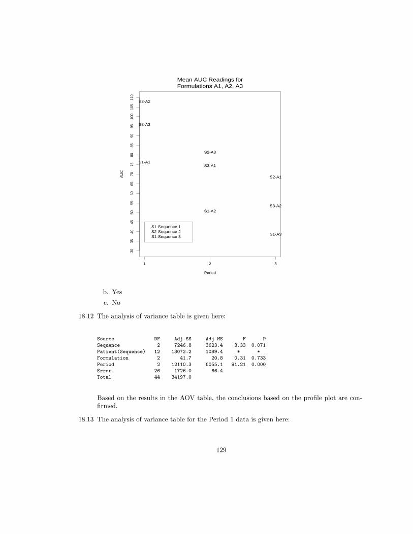
Mean AUC Readings forFormulations A1, A2, A3
Period
AU
C
1 2 3
3035
4045
5055
6065
7075
8085
9095
100
105
110
S1-A1
S1-A2
S1-A3
S2-A2
S2-A3
S2-A1
S3-A3
S3-A1
S3-A2
S1-Sequence 1S2-Sequence 2S1-Sequence 3
b. Yes
c. No
18.12 The analysis of variance table is given here:
Source DF Adj SS Adj MS F P
Sequence 2 7246.8 3623.4 3.33 0.071
Patient(Sequence) 12 13072.2 1089.4 * *
Formulation 2 41.7 20.8 0.31 0.733
Period 2 12110.3 6055.1 91.21 0.000
Error 26 1726.0 66.4
Total 44 34197.0
Based on the results in the AOV table, the conclusions based on the profile plot are con-firmed.
18.13 The analysis of variance table for the Period 1 data is given here:
129

Source DF Adj SS Adj MS F P
Formulation 2 2553.8 1276.9 2.51 0.123
Error 12 6112.6 509.4
Total 14 8666.4
A similar result is obtained using just the first Period, there is not an effect due to due tothe formulations (p− value = 0.123). The crossover design used in Exercise 18.12 is moresuitable because the variability in response from individual patients is reduced by havingeach patient respond to each of the three formulations.
18.17 a. The mean efficiencies for each model at each time point are given here:
TimeModel 1 2 3 4 5
1 1.72 1.68 1.75 1.76 1.722 1.95 1.90 2.01 2.05 1.99
A plot of the mean efficiences is given here:
1
1
11
1
2
2
2
2
2
Mean Efficiency Rating forModel 1, Model 2
Time (Hours)
Mean
Effic
iency
Rati
ngs
1 2 3 4 5
1.55
1.60
1.65
1.70
1.75
1.80
1.85
1.90
1.95
2.00
2.05
2.10
1 - Model 12 - Model 2
b. The analysis of variance table in the textbook yields the following results:
The adjusted p-value for the Time by Model interaction is 0.7528.
The p-value for the main effect of Model is 0.0960 which indicates that there is notsignificant evidence of a difference between the two models with respect to meanefficiency ratings.
The adjusted p-value for the main effect due to Time is 0.0512 which indicates thereis not significant evidence of a difference in the mean efficiency ratings across the fivetime periods.
130
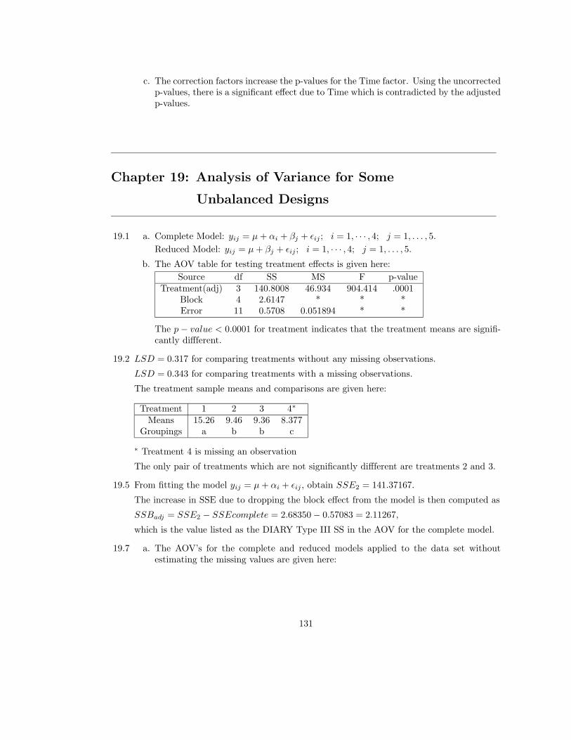
c. The correction factors increase the p-values for the Time factor. Using the uncorrectedp-values, there is a significant effect due to Time which is contradicted by the adjustedp-values.
Chapter 19: Analysis of Variance for Some
Unbalanced Designs
19.1 a. Complete Model: yij = µ+ αi + βj + εij ; i = 1, · · · , 4; j = 1, . . . , 5.
Reduced Model: yij = µ+ βj + εij ; i = 1, · · · , 4; j = 1, . . . , 5.
b. The AOV table for testing treatment effects is given here:
Source df SS MS F p-valueTreatment(adj) 3 140.8008 46.934 904.414 .0001
Block 4 2.6147 * * *Error 11 0.5708 0.051894 * *
The p− value < 0.0001 for treatment indicates that the treatment means are signifi-cantly diffferent.
19.2 LSD = 0.317 for comparing treatments without any missing observations.
LSD = 0.343 for comparing treatments with a missing observations.
The treatment sample means and comparisons are given here:
Treatment 1 2 3 4∗
Means 15.26 9.46 9.36 8.377Groupings a b b c
∗ Treatment 4 is missing an observation
The only pair of treatments which are not significantly diffferent are treatments 2 and 3.
19.5 From fitting the model yij = µ+ αi + εij , obtain SSE2 = 141.37167.
The increase in SSE due to dropping the block effect from the model is then computed as
SSBadj = SSE2 − SSEcomplete = 2.68350− 0.57083 = 2.11267,
which is the value listed as the DIARY Type III SS in the AOV for the complete model.
19.7 a. The AOV’s for the complete and reduced models applied to the data set withoutestimating the missing values are given here:
131
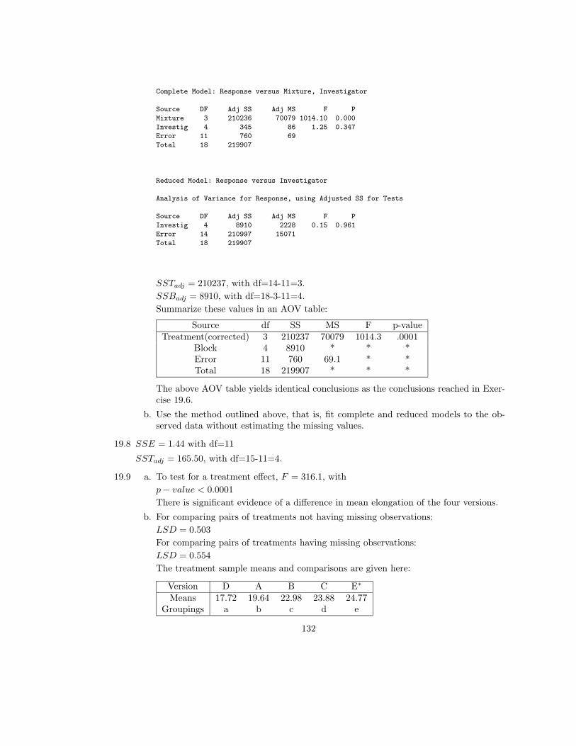
Complete Model: Response versus Mixture, Investigator
Source DF Adj SS Adj MS F P
Mixture 3 210236 70079 1014.10 0.000
Investig 4 345 86 1.25 0.347
Error 11 760 69
Total 18 219907
Reduced Model: Response versus Investigator
Analysis of Variance for Response, using Adjusted SS for Tests
Source DF Adj SS Adj MS F P
Investig 4 8910 2228 0.15 0.961
Error 14 210997 15071
Total 18 219907
SSTadj = 210237, with df=14-11=3.
SSBadj = 8910, with df=18-3-11=4.
Summarize these values in an AOV table:
Source df SS MS F p-valueTreatment(corrected) 3 210237 70079 1014.3 .0001
Block 4 8910 * * *Error 11 760 69.1 * *Total 18 219907 * * *
The above AOV table yields identical conclusions as the conclusions reached in Exer-cise 19.6.
b. Use the method outlined above, that is, fit complete and reduced models to the ob-served data without estimating the missing values.
19.8 SSE = 1.44 with df=11
SSTadj = 165.50, with df=15-11=4.
19.9 a. To test for a treatment effect, F = 316.1, with
p− value < 0.0001
There is significant evidence of a difference in mean elongation of the four versions.
b. For comparing pairs of treatments not having missing observations:
LSD = 0.503
For comparing pairs of treatments having missing observations:
LSD = 0.554
The treatment sample means and comparisons are given here:
Version D A B C E∗
Means 17.72 19.64 22.98 23.88 24.77Groupings a b c d e
132
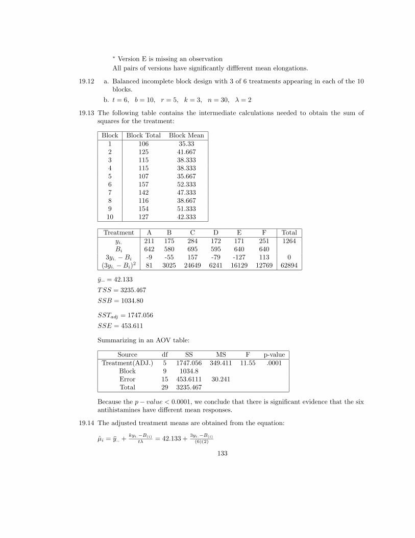
∗ Version E is missing an observation
All pairs of versions have significantly diffferent mean elongations.
19.12 a. Balanced incomplete block design with 3 of 6 treatments appearing in each of the 10blocks.
b. t = 6, b = 10, r = 5, k = 3, n = 30, λ = 2
19.13 The following table contains the intermediate calculations needed to obtain the sum ofsquares for the treatment:
Block Block Total Block Mean1 106 35.332 125 41.6673 115 38.3334 115 38.3335 107 35.6676 157 52.3337 142 47.3338 116 38.6679 154 51.33310 127 42.333
Treatment A B C D E F Totalyi. 211 175 284 172 171 251 1264Bi 642 580 695 595 640 640
3yi. −Bi -9 -55 157 -79 -127 113 0(3yi. −Bi)2 81 3025 24649 6241 16129 12769 62894
y.. = 42.133
TSS = 3235.467
SSB = 1034.80
SSTadj = 1747.056
SSE = 453.611
Summarizing in an AOV table:
Source df SS MS F p-valueTreatment(ADJ.) 5 1747.056 349.411 11.55 .0001
Block 9 1034.8Error 15 453.6111 30.241Total 29 3235.467
Because the p− value < 0.0001, we conclude that there is significant evidence that the sixantihistamines have different mean responses.
19.14 The adjusted treatment means are obtained from the equation:
µi = y.. +kyi.−B(i)
tλ = 42.133 +3yi.−B(i)
(6)(2)
133
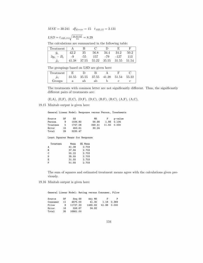
MSE = 30.241 dfError = 15 t.025,15 = 2.131
LSD = t.025,15
√2kMSEtλ = 8.29
The calculations are summarized in the following table:
Treatment A B C D E Fyi. 42.2 35 56.8 34.4 34.2 50.2
3yi. −Bi -9 -55 157 -79 -127 113µi 41.38 37.55 55.22 35.55 31.55 51.54
The groupings based on LSD are given here:
Treatment E D B A F Cµi 31.55 35.55 37.55 41.38 51.54 55.22
Groups a ab ab b c c
The treatments with common letter are not significantly different. Thus, the significantlydifferent pairs of treatments are:
(E,A), (E,F), (E,C), (D,F), (D,C), (B,F), (B,C), (A,F), (A,C),
19.15 Minitab output is given here:
General Linear Model: Response versus Person, Treatments
Source DF SS MS F p-value
Person 9 1034.80 56.98 1.88 0.134
Treatmen 5 1747.06 349.41 11.55 0.000
Error 15 453.61 30.24
Total 29 3235.47
Least Squares Means for Response
Treatmen Mean SE Mean
A 41.38 2.703
B 37.55 2.703
C 55.22 2.703
D 35.55 2.703
E 31.55 2.703
F 51.55 2.703
The sum of squares and estimated treatment means agree with the calculations given pre-viously.
19.16 Minitab output is given here:
General Linear Model: Rating versus Consumer, Pilow
Source DF Seq SS Adj MS F P
Consumer 11 4575.00 41.30 1.18 0.369
Pilow 8 11727.33 1465.92 41.98 0.000
Error 16 558.67 34.92
Total 35 16861.00
134
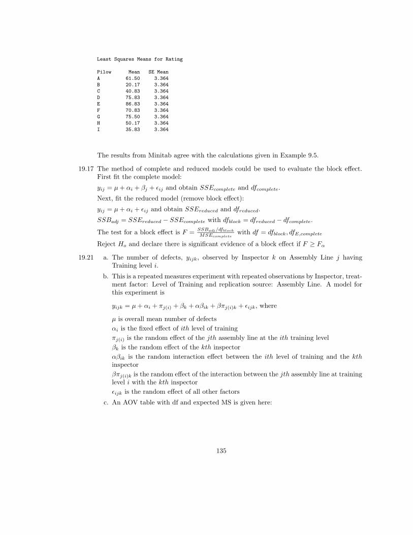
Least Squares Means for Rating
Pilow Mean SE Mean
A 61.50 3.364
B 20.17 3.364
C 40.83 3.364
D 75.83 3.364
E 86.83 3.364
F 70.83 3.364
G 75.50 3.364
H 50.17 3.364
I 35.83 3.364
The results from Minitab agree with the calculations given in Example 9.5.
19.17 The method of complete and reduced models could be used to evaluate the block effect.First fit the complete model:
yij = µ+ αi + βj + εij and obtain SSEcomplete and dfcomplete.
Next, fit the reduced model (remove block effect):
yij = µ+ αi + εij and obtain SSEreduced and dfreduced.
SSBadj = SSEreduced − SSEcomplete with dfblock = dfreduced − dfcomplete.The test for a block effect is F =
SSBadj/dfblockMSEcomplete
with df = dfblock, dfE,complete
Reject Ho and declare there is significant evidence of a block effect if F ≥ Fα19.21 a. The number of defects, yijk, observed by Inspector k on Assembly Line j having
Training level i.
b. This is a repeated measures experiment with repeated observations by Inspector, treat-ment factor: Level of Training and replication source: Assembly Line. A model forthis experiment is
yijk = µ+ αi + πj(i) + βk + αβik + βπj(i)k + εijk, where
µ is overall mean number of defects
αi is the fixed effect of ith level of training
πj(i) is the random effect of the jth assembly line at the ith training level
βk is the random effect of the kth inspector
αβik is the random interaction effect between the ith level of training and the kthinspector
βπj(i)k is the random effect of the interaction between the jth assembly line at traininglevel i with the kth inspector
εijk is the random effect of all other factors
c. An AOV table with df and expected MS is given here:
135

Source df Expected MSTraining 1 σ2
ε + 2σ2L(T )∗I + 6σ2
T∗I + 12σ2I + 4σ2
L(T ) + 12QTLine(Training) 4 σ2
ε + 2σ2L(T )∗I + 4σ2
L(T )
Inspector 1 σ2ε + 2σ2
L(T )∗I + 12σ2I
Training*Inspector 1 σ2ε + 2σ2
L(T )∗I + 6σ2T∗I
Line(Training)*Inspector 4 σ2ε + 2σ2
L(T )∗IError 12 σ2
ε
Total 23
19.22 a. We can use a mixed models approach to test the relevant hypotheses.
b. The interaction between Training and Inspector and the main effects due to Train-ing and Inspector. Since the random effect of Line(Training)*Inspector is essentially
neglible, the term σ2L(T )∗I will be set to zero. In fact, σ2
L(T )∗I =MSL(T )∗I−MSE
2 =1.333−105
2 = −51.83, which is set equal to 0. Taking into account the resulting changein the expected MS’s, we obtain the following test statistics:
Training*Inspector: F = MST∗IMSE = 1.5/1
105/12 = 0.17⇒ p− value = 0.6861⇒There is not significant evidence of an interaction effect between Inspectors and Train-ing.
Training: To determine the test statistic for testing the main effect due to training weneed to examine the expected MS column. We note that under the null hypothesis ofno main effect due to Training, QT = 0. This implies that under the null hypothesisof no main effect due to training that
EMST = EMSL(T ) + EMSI + EMST∗I − 3 ∗ EMSE
Thus, the denominator of our test statistic is
MSL(T ) +MSI +MST∗I − 3 ∗MSE = 14.17 + 0.67 + 1.5− 3(8.750) = −9.91.
This would be meaningless, hence we will use as an approximation the following teststatistic.
F = MSTMSE = 130.67
8.750 = 14.93⇒ p− value = 0.0023.
There is significant evidence of an effect due to Training. That is, the AdditionalTraining appears to have reduced the mean number of defects.
Similarly we obtain there is not a significant effect due to Inspectors (p − value =0.7872).
c. A profile plot of the mean number of defects for the levels of training is give here:
136
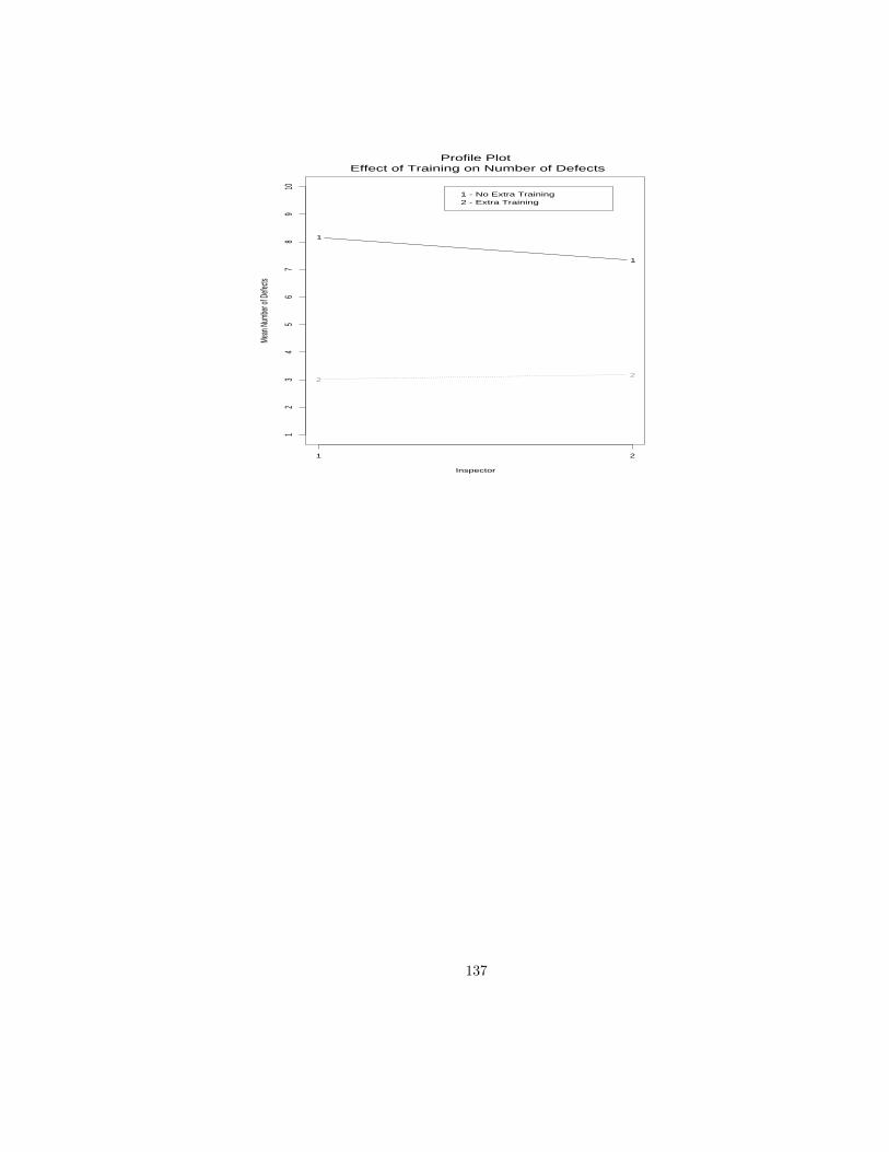
1
1
22
Profile Plot Effect of Training on Number of Defects
Inspector
Mean
Num
ber o
f Defe
cts
1 2
12
34
56
78
910
1 - No Extra Training2 - Extra Training
137