Embed Size (px)
Citation preview

AnswerstoApplicationActivitiesinChapter9
10.5.5ApplicationActivitywithOne‐WayANOVAs1 Ellis and Yuan (2004)
Use the dataset EllisYuan.sav. Import into R as EllisYuan.
a.CheckAssumptionsWe assume that the variables were independently gathered. Use boxplots and histograms as well
as numerical values for skewness and kurtosis to check on normality assumptions and
homogeneity of variances.
SPSS Instructions:
For boxplots, histograms and numerical values from one command, choose ANALYZE >
DESCRIPTIVE STATISTICS > EXPLORE. Put the three variables of ERRORFREECLAUSES, MSTTR
and SPM in the “Dependent List.” Put Group in the “Factor List.” Open the “Plots” button and
tick on “Histogram” and “Normality plots with tests.” Press Continue and then OK. The Explore
command produces a lot of output, so the results won't list all of it, just my overall summary of
results.
R Instructions:
To look at normality graphically and numerically, first make sure EllisYuan is the active dataset.
First let’s look at boxplots. In R Commander, choose GRAPHS > BOXPLOT, and then choose
errorfreeclauses. Open the “Plot by groups” button and group will already be chosen, so just

press OK. You can press the “Apply” button instead of “OK” in the main dialogue box, which
will let you then choose the other two variables (msttr, spm) in turn. Press OK when you are
finished. The R code for the first variable is:
Boxplot(errorfreeclauses~group, data=EllisYuan, id.method="y")
Now look at histograms. In R Commander, choose GRAPHS > HISTOGRAM, and then choose
errorfreeclauses. Open the “Plot by groups” button and group will already be chosen, so just
press OK. You can press the “Apply” button instead of “OK” in the main dialogue box, which
will let you then choose the other two variables (msttr, spm) in turn. Press OK when you are
finished. The R code for the first variable is:
with(EllisYuan, Hist(errorfreeclauses, groups=group, scale="frequency",
breaks="Sturges", col="darkgray"))
Last, to look at numbers like skewness and kurtosis the fBasics package provides a lot of
numbers, but the basicStats( ) command does not provide a way to break up the data by group,
so we will have to do that manually by examining what rows each group is found in. I opened up
the button on the R Commander GUI “View dataset” and found that the NP group used rows 1-
14, PTP rows 15–28, and OLP rows 29–42. By the way, the R code to do this if you do not use R
Commander is:
showData(EllisYuan, placement='-20+200', font=getRcmdr('logFont'),

maxwidth=80, maxheight=30)
Now knowing these rows, I can implement the command for each of the three groups for each of
the three variables I want to look at:
library(fBasics) #open package
attach(EllisYuan) #lets me type the variable without specifying the dataset
basicStats(errorfreeclauses[1:14])
basicStats(errorfreeclauses[15:28])
basicStats(errorfreeclauses[29:42])
Repeat with the other variables and at the end:
detach(EllisYuan)
Results:
I won’t list all of it, but my general summary for the normality assumptions for each variable is
given below:
1 ERRORFREECLAUSES: the NP group has non-normal distribution (skewness and kurtosis
numbers are high), and both NP and PTP have outliers (as seen in the boxplot). Variances
seem to be unequal (as seen in the boxplot).

2 MSTTR: the PTP group has outliers (as seen in the boxplot). Variances seem to be
unequal (as seen in the boxplot). Variances seem to be unequal (as seen in the boxplot).
3 SPM: the PTP group is skewed (skewness and kurtosis numbers are high, histogram is
skewed, boxplot not symmetrically distributed) and has an outlier (as seen in the boxplot).
The OLP group is also skewed (histogram and boxplot). Variances seem to be unequal
(as seen in the boxplot).
b.RuntheOne‐wayANOVASPSS Instructions:
Open ANALYZE > COMPARE MEANS > ONE-WAY ANOVA. Put SPM, LEXICAL VARIETY OR MSTTR,
and ERROR-FREE CLAUSES in the “Dependent List” box and GROUP in the “Factor” box. In the
POST HOC area you can choose which post-hoc tests to use, if you want to use any at all (if using
the “old statistics” approach, my recommendation is to open the POST HOC button and tick LSD,
which does not adjust means, and also tick Games-Howell because variances are not equal. Press
Continue).
Open the Options button and tick “Descriptive” and “Homogeneity of variances test.” Press
CONTINUE. Press OK and run the test.
R Instructions:
In R Commander, make sure EllisYuan is the active dataset. Choose STATISTICS > MEANS >
ONE-WAY ANOVA. Choose group (=independent variable) and errorfreeclauses (=dependent
variable). Tick the box for pairwise comparison of means. Change the name of the regression
model if you like. You can press the “Apply” button instead of “OK” in the main dialogue box,
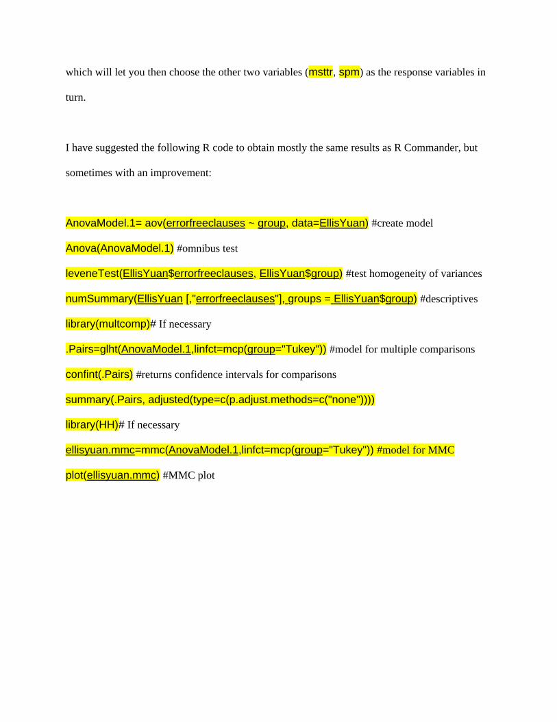
which will let you then choose the other two variables (msttr, spm) as the response variables in
turn.
I have suggested the following R code to obtain mostly the same results as R Commander, but
sometimes with an improvement:
AnovaModel.1= aov(errorfreeclauses ~ group, data=EllisYuan) #create model
Anova(AnovaModel.1) #omnibus test
leveneTest(EllisYuan$errorfreeclauses, EllisYuan$group) #test homogeneity of variances
numSummary(EllisYuan [,"errorfreeclauses"], groups = EllisYuan$group) #descriptives
library(multcomp)# If necessary
.Pairs=glht(AnovaModel.1,linfct=mcp(group="Tukey")) #model for multiple comparisons
confint(.Pairs) #returns confidence intervals for comparisons
summary(.Pairs, adjusted(type=c(p.adjust.methods=c("none"))))
library(HH)# If necessary
ellisyuan.mmc=mmc(AnovaModel.1,linfct=mcp(group="Tukey")) #model for MMC
plot(ellisyuan.mmc) #MMC plot

Results:
Result are taken from SPSS (confidence intervals differ slightly from R)
Omnibus F test
Mean difference for NP-PTP + CI of mean difference (using LSD post-hoc, in other words, no adjustment)
Mean difference for NP-OLP + CI of mean difference (LSD)
Mean difference for OLP-PTP + CI of mean difference (LSD)
SPM F2,39=11.19, p=.000
-3.77 (-5.83, -1.70)
.73 (-1.34, 2.79) -4.50 (-6.56, -2.43)
MSTTR (lexical variety)
F2,39=.18, p=.84
-.001 (-.02, .02) .005 (-.02, .03) -.006 (-.03, .02)
Error-free clauses
F2,39=3.04, p=.06
-.03 (-.11, .04) .09 (-.17, -.2) .06 (-.02, .13)
Effect sizes are calculated using means and pooled standard deviations for each group with an
online calculator.
Mean NP N=14
Mean PTP N=14
Mean OLP N=14
ES for NP-PTP
ES for NP-OLP
ES for PTP-OLP
ES for NP-PTP
SPM
12.5 (2.0) 16.3 (3.3) 11.8 (2.7) -1.39 .29 1.49 -1.39
MSTTR
.88 (.03) .88 (.02) .87 (.03) 0 .33 .39 0
Error-free clauses
.77 (.10) .81 (.12) .86 (.07) -.36 -1.04 -.51 -.36
Remarks:
It’s interesting that planning time had no effect on lexical variety (MSTTR). It’s interesting to
look at effect sizes here and see what effect sizes are found even when differences between
groups are very small. For speed, the difference between the No Planning and Online Planning
group has a large effect size and is statistical (even though the omnibus is not quite under p=.05!).
For error-free clauses, it seems that pre-task planning had a large effect on improving the number
of these.

2 Pandey (2000)
Use the Pandey2000.sav file. Import into R as Pandey.
a.CheckAssumptionsWe assume that the variables were independently gathered. Use histograms as well as numerical
values for skewness and kurtosis to check on normality assumptions and homogeneity of
variances.
SPSS Instructions:
For boxplots, histograms and numerical values from one command, choose ANALYZE >
DESCRIPTIVE STATISTICS > EXPLORE. Put the variable of GAIN1in the “Dependent List”. Put
Group in the “Factor List”. Open the “Plots” button and tick on “Histogram” and “Normality
plots with tests.” Press Continue and then OK. The Explore command produces a lot of output,
so the results won't list all of it, just my overall summary of results.
R Instructions:
To look at normality graphically and numerically, first make sure Pandey is the active dataset.
First let’s look at boxplots. In R Commander, choose GRAPHS > BOXPLOT, and then choose
gain1. Open the “Plot by groups” button and group will already be chosen, so just press OK.
Press OK again to run the command. The R code is:
Boxplot(gain1~group, data=Pandey, id.method="y")

Now look at histograms. In R Commander, choose GRAPHS > HISTOGRAM, and then choose
gain1. Open the “Plot by groups” button and group will already be chosen, so just press OK.
Press OK to run the command. The R code is:
with(Pandey, Hist(gain1, groups=group, scale="frequency", breaks="Sturges",
col="darkgray"))
Last, to look at numbers like skewness and kurtosis the fBasics package provides a lot of
numbers, but the basicStats( ) command does not provide a way to break up the data by group,
so we will have to do that manually by examining what rows each group is found in. I opened up
the button on the R Commander GUI “View dataset” and found that the Focus A group used
rows 1–11, Focus B rows 12–23, and ControlA rows 24–45. By the way, the R code to do this if
you do not use R Commander is:
showData(Pandey, placement='-20+200', font=getRcmdr('logFont'), maxwidth=80,
maxheight=30)
Now knowing these rows, I can implement the command for each of the three groups for each of
the three variables I want to look at:
library(fBasics)# open package
attach(Pandey)# lets me type the variable without specifying the dataset
basicStats(gain1[1:11])

basicStats(gain1[12:23])
basicStats(gain1[24:45])
detach(Pandey)
Results:
In the first gain score, Focus group B is a little bit skewed, and the control group has many
outliers, judging by the boxplot. The histograms from Focus A and Focus B could be normal
distributions, but the Control A histogram looks very non-normal. The skewness and kurtosis
numbers for the groups are OK for Focus A and Focus B but large for Control A. From the
boxplot we see that the control group’s variance is certainly much different from either Focs A or
Focus B, and the variance of Focus A looks different from Focus B.
b.RuntheOne‐wayANOVASPSS Instructions:
Open ANALYZE > COMPARE MEANS > ONE-WAY ANOVA. Put GAIN1 in the “Dependent List” box
and GROUP in the “Factor” box. For planned comparisons, open the CONTRASTS button. Our first
contrast will look at just Group A compared to Group B, so the coefficients to enter will be: 1, -1,
0. After entering each number, press the “Add” button. After entering all three numbers, press
the “Next” button. The next contrast will be Group A and Group B contrasted against Control, so
enter: 1, 1, -2. Press CONTINUE. Open the Options button and tick “Descriptive” and
“Homogeneity of variances test”. Press CONTINUE. Press OK to run the analysis.
R Instructions:
Refer to Section 9.4.8 of the book. First, I want to set up the contrasts:
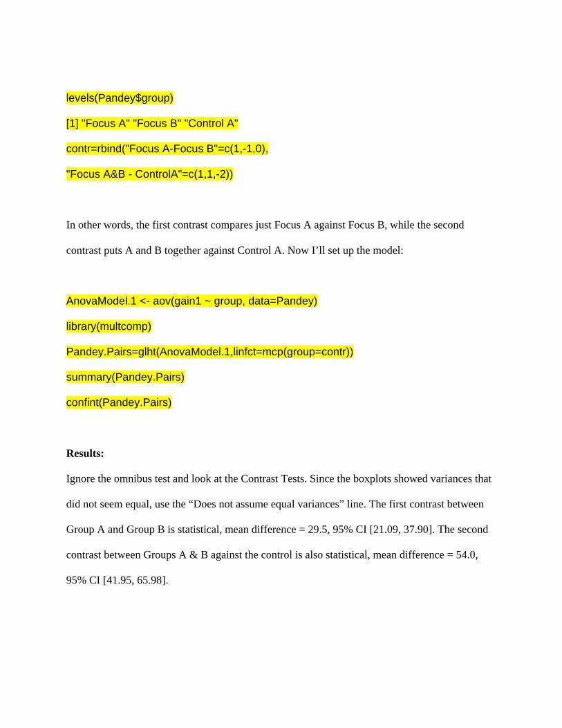
levels(Pandey$group)
[1] "Focus A" "Focus B" "Control A"
contr=rbind("Focus A-Focus B"=c(1,-1,0),
"Focus A&B - ControlA"=c(1,1,-2))
In other words, the first contrast compares just Focus A against Focus B, while the second
contrast puts A and B together against Control A. Now I’ll set up the model:
AnovaModel.1 <- aov(gain1 ~ group, data=Pandey)
library(multcomp)
Pandey.Pairs=glht(AnovaModel.1,linfct=mcp(group=contr))
summary(Pandey.Pairs)
confint(Pandey.Pairs)
Results:
Ignore the omnibus test and look at the Contrast Tests. Since the boxplots showed variances that
did not seem equal, use the “Does not assume equal variances” line. The first contrast between
Group A and Group B is statistical, mean difference = 29.5, 95% CI [21.09, 37.90]. The second
contrast between Groups A & B against the control is also statistical, mean difference = 54.0,
95% CI [41.95, 65.98].

3 Thought Question
The main problem with this design is that it is repeated measures, so data is not independent. If
the researcher were to ask whether there were any difference between groups for only ONE of
the three discourse completion tasks, assuming that each of the 3 classes received different
treatments, this would be a valid one-way ANOVA. You might think this experiment looks a lot
like the Pandey experiment in #2, and that is right, but in that case we looked at a gain score
from Time 2 to Time 1. Doing a one-way ANOVA in this case on one gain score would be fine
(say, the gain from DCT Time 2 minus DCT Time 1) but to try to put the scores of all three
discourse completion tasks together and then perform a one-way ANOVA would compromise
the fundamental assumption of independence of groups in the one-way ANOVA.
4 Inagaki and Long (1999)
Use the InagakiLong.sav file. Import into R as InagakiLong.
a.CheckAssumptionsWe assume that the variables were independently gathered. Use histograms as well as numerical
values for skewness and kurtosis to check on normality assumptions and homogeneity of
variances.
SPSS Instructions:
For boxplots, histograms and numerical values from one command, choose ANALYZE >
DESCRIPTIVE STATISTICS > EXPLORE. Put the two variables of GAINADJ and GAINLOC in the
“Dependent List”. Put GROUP in the “Factor List”. Open the “Plots” button and tick on

“Histogram” and “Normality plots with tests”. Press Continue and then OK. The Explore
command produces a lot of output, so the results won’t list all of it, just my overall summary of
results.
R Instructions:
To look at normality graphically and numerically, first make sure InagakiLong is the active
dataset. First let’s look at boxplots. In R Commander, choose GRAPHS > BOXPLOT, and then
choose gainadj. Open the “Plot by groups” button and group will already be chosen, so just
press OK. You can press the “Apply” button instead of “OK” in the main dialogue box, which
will let you then choose the other variable (gainloc) in turn. Press OK when you are finished.
The R code for the first variable is:
Boxplot(gainadj~group, data=InagakiLong, id.method="y")
Now look at histograms. In R Commander, choose GRAPHS > HISTOGRAM, and then choose
gainadj. Open the “Plot by groups” button and group will already be chosen, so just press OK.
You can press the “Apply” button instead of “OK” in the main dialogue box, which will let you
then choose the other variable (gainloc) in turn. Press OK when you are finished. The R code for
the first variable is:
with(InagakiLong, Hist(gainadj, groups=group, scale="frequency",
breaks="Sturges", col="darkgray"))

Last, to look at numbers like skewness and kurtosis the fBasics package provides a lot of
numbers, but the basicStats( ) command does not provide a way to break up the data by group,
so we will have to do that manually by examining what rows each group is found in. I opened up
the button on the R Commander GUI “View dataset” and found that the Model group used rows
1–8, Recast rows 9–16, and Control rows 17–24 (the sample size is rather small). By the way,
the R code to do this if you do not use R Commander is:
showData(InagakiLong, placement='-20+200', font=getRcmdr('logFont'),
maxwidth=80, maxheight=30)
Now knowing these rows, I can implement the command for each of the three groups for each of
the three variables I want to look at:
library(fBasics)# open package
attach(InagakiLong)# lets me type the variable without specifying the dataset
basicStats(gainadj[1:8])
basicStats(gainadj [9:16])
basicStats(gainadj [17:24])
Repeat with the other variable and at the end:
detach(InagakiLong)

Results:
GainAdj: The boxplots and histograms show that all groups are skewed, and the control group
did not make any gain, so they have no variance (there is just one outlier though). They should
not be compared to the other two groups for adjectives. The skewness numbers are below 1
except for the Control group, which has a skewness of 1.9.
GainLoc: The boxplots and histograms show that all groups are skewed. The variance of the
Model group is much larger than that of the Recast or Control group. The skewness numbers are
slightly above 1 for all the groups, so we can say these variables are not normally distributed.
b.RuntheOne‐wayANOVAThe previous look at the variables show that we cannot run a one-way ANOVA on the gainscore
on adjectives since there is no variation in the Control group. We would be able to run a t-test on
this data, comparing the Model and Recast groups; however, I will not do that here.
SPSS Instructions:
Open ANALYZE > COMPARE MEANS > ONE-WAY ANOVA. Put GAINLOC in the “Dependent List”
box and GROUP in the “Factor” box. In the POST HOC area you can choose which post-hoc tests
to use, if you want to use any at all (if using the “old statistics” approach, my recommendation is
to open the POST HOC button and tick LSD, which does not adjust means, and also tick Games-
Howell because variances are not equal. Press Continue).
Open the Options button and tick “Descriptive” and “Homogeneity of variances test”. Press
CONTINUE. We want robust tests, so open the BOOTSTRAP button and check the “Perform
bootstrapping” box, change the number of samples to 10,000 (or possibly less if you don’t have

much time to wait), and change the “Confidence Intervals” to BCa. Press CONTINUE then OK
and run the test.
To calculate effect sizes, use an online calculator with the mean scores and standard deviations.
R Instructions:
In R Commander, make sure InagakiLong is the active dataset. Choose STATISTICS > MEANS >
ONE-WAY ANOVA. Choose group (=independent variable) and gainloc (=dependent variable).
Tick the box for pairwise comparison of means. Change the name of the regression model if you
like. Press OK.
I have suggested the following R code to obtain mostly the same results as R Commander, but
sometimes with an improvement:
AnovaModel.1= aov(gainloc ~ group, data=InagakiLong) #create model
Anova(AnovaModel.1) #omnibus test
leveneTest(InagakiLong$gainloc, InagakiLong$group) #test homogeneity of variances
numSummary(InagakiLong [,"gainloc"], groups = InagakiLong$group) #descriptives
library(multcomp) #If necessary
.Pairs=glht(AnovaModel.1,linfct=mcp(group="Tukey")) #model for multiple comparisons
confint(.Pairs) #returns confidence intervals for comparisons
summary(.Pairs, adjusted(type=c(p.adjust.methods=c("none"))))
library(HH) #if necessary

ellisyuan.mmc=mmc(AnovaModel.1,linfct=mcp(group="Tukey")) #model for MMC
plot(ellisyuan.mmc) #MMC plot
For a Bootstrapped One-way ANOVA
Note that the only place where this syntax would change is in the underlined and red
portions
library(boot)# open the package
MeanDifference <- function (data,i){
temp<-data[i,]
aov.temp<-aov(gainloc ~ group, data=temp)
Tuk <-TukeyHSD(aov.temp)
return(Tuk$group[,1])
}
MeanDifferenceBoot <- boot(InagakiLong, MeanDifference, 10000)
#if 10000 takes too long you can change the number of
#replicates to a smaller number (press the Escape key to stop the command)
PAIRci.s <- NULL
PAIRt0 <- as.data.frame(MeanDifferenceBoot[1])
for(i in 1:length(MeanDifferenceBoot[[1]])){
CI <- boot.ci(MeanDifferenceBoot, conf = .95,
type = "bca", t0 = MeanDifferenceBoot$t0[i] ,

t = MeanDifferenceBoot$t[,i])
PAIRci.s[[paste("lwr",i,sep=".")]]<- CI$bca[c(4)]
PAIRci.s[[paste("upr",i,sep=".")]]<- CI$bca[c(5)]
}
Pci <- matrix(PAIRci.s, ncol = 2, nrow = length(PAIRt0[[1]]),
byrow=TRUE)
PAIRboot.ci <- data.frame(PAIRt0[1], lwr = Pci[, 1], upr = Pci[, 2])
print(PAIRboot.ci)
To calculate Cohen’s d effect size (and associated confidence intervals around this effect size),
use the following code:
bootES(InagakiLong, R=2000, data.col="gainloc", group.col="group",
contrast=c(Recast=1, Model=-1),effect.type=c("cohens.d"), ci.type=c("bca"))
Repeat with the other pairings of variables:
contrast=c(Recast=1, Control=-1)
contrast=c(Model=1, Control=-1)

Results:
For subject placement after a locative phrase, the following results were found using R:
Omnibus F test
Mean difference for Recast-Model + CI of mean difference (using LSD post-hoc, in other words, no adjustment)
Mean difference for Control-Model + CI of mean difference (LSD)
Mean difference for Control-Recast + CI of mean difference (LSD)
GainLoc F2,21=0.37, p=.695
0.38 [-1.64, 0.89]
0.38 [-1.64, 0.89]
.000 [-1.27, 1.27]
Boot- strapped CIs
[-1.52, 0.56] [-1.56, 0.50] [-0.70, 0.73]
Mean Recast N=8
Mean Model N=8
Mean Control N=8
ES for Recast-Model (CI)
ES for Control- Model (CI)
ES for Control- Recast (CI)
GainLoc 0.38 (.74) 0.75 (1.39) 0.38 (.74) .34 [-1.32, 0.76]
.34 [-0.94, 1.32]
0.00 [-1.20, 0.84]
The overall omnibus test is not statistical, F2,21 = .37, p = .69. In the “old statistics” this would be
the end and we wouldn’t look any further. However, we are interested in reporting confidence
intervals, so we’ll continue on to look at the pairings between groups.
The confidence intervals all pass through zero and are pretty much centered around zero. It is
true that sample sizes are small, but the confidence intervals show that even with repeated testing,
no effect would be likely to be found for differences between the experimental groups. I note that
one possible problem with this study was that only 3 items per structure were used. There might
have been more differentiation with a larger number of items!
Lastly, effect sizes for all pairings are small, with confidence intervals for the effect sizes going
through zero and showing that the estimate is not very precise.

5 Dewaele and Pavlenko (2001–2003)
Use the BEQ.Context.sav file. Import into R as beq.context.
a.CheckAssumptionsWe assume that the variables were independently gathered. Use histograms as well as numerical
values for skewness and kurtosis to check on normality assumptions and homogeneity of
variances. See Exercise #1 and Exercise #4 for similar datasets. Since you have detailed
instructions in those exercises, I will only give bare bones instructions for this dataset.
SPSS Instructions:
In the EXPLORE option, put the two variables of L2SPEAK and L2_READ in the “Dependent List.”
Put L2CONTEXT in the “Factor List.”
R Instructions:
Boxplot(l2speak~l2context, data=beq.context, id.method="y")
Boxplot(l2_read~l2context, data=beq.context, id.method="y")
with(beq.context, Hist(l2speak, groups=l2context, scale="frequency",
breaks="Sturges", col="darkgray"))
with(beq.context, Hist(l2_read, groups=l2context, scale="frequency",
breaks="Sturges", col="darkgray"))
I need to break up the dataset into groups, but they are not all in 3 easy divisions, so I’ll use code
to do it:
levels(beq.context$l2context)

[1] "Instructed" "Naturalistic"
[3] "Both instructed and naturalistic"
beqNatural <- subset(beq.context, subset=l2context=="Naturalistic")
beqInstr <- subset(beq.context, subset=l2context=="Instructed")
beqBoth <- subset(beq.context, subset=l2context=="Both instructed and naturalistic")
Having these divisions I can implement the command for each of the three groups for each of the
three variables I want to look at:
library(fBasics) #open package
basicStats(beqNatural$l2speak)
basicStats(beqInstr$l2speak)
basicStats(beqBoth$l2speak)
Repeat with the other variable (l2_read).
Results:
For speaking and reading, looking at boxplots and histograms, all data are skewed, with more
results toward 5 than would be predicted by a normal distribution, and there are outliers. For
reading, all groups have equal variances (looking at boxplots). For speaking, the instructed
learners have a bigger variance than the other two groups (looking at boxplots). For speaking,
every group except instructed learners have skewness numbers over 1. For reading, all groups
have skewness numbers over 1. Variables are certainly not normally distributed.

b.RuntheOne‐wayANOVASPSS Instructions:
In the ONE-WAY ANOVA box, put L2SPEAK and L2_READ in the “Dependent List” box and
L2CONTEXT in the “Factor” box.
To calculate effect sizes, use an online calculator with the mean scores and standard deviations.
R Instructions:
AnovaModel.1= aov(l2speak ~ l2context, data=beq.context)
Anova(AnovaModel.1)
Repeat with other variable (l2_read).
numSummary(beq.context [,"l2speak"], groups = beq.context$l2context)
Repeat with other variable (l2_read).
.Pairs=glht(AnovaModel.1,linfct=mcp(l2context="Tukey"))
confint(.Pairs)
Repeat with other variable (l2_read).
For a Bootstrapped One-way ANOVA

MeanDifference <- function (data,i){
temp<-data[i,]
aov.temp<-aov(l2speak ~ l2context, data=temp)
Tuk <-TukeyHSD(aov.temp)
return(Tuk$l2context[,1])
}
MeanDifferenceBoot <- boot(beq.context, MeanDifference, 2000)
PAIRci.s <- NULL
PAIRt0 <- as.data.frame(MeanDifferenceBoot[1])
for(i in 1:length(MeanDifferenceBoot[[1]])){
CI <- boot.ci(MeanDifferenceBoot, conf = .95,
type = "bca", t0 = MeanDifferenceBoot$t0[i] ,
t = MeanDifferenceBoot$t[,i])
PAIRci.s[[paste("lwr",i,sep=".")]]<- CI$bca[c(4)]
PAIRci.s[[paste("upr",i,sep=".")]]<- CI$bca[c(5)]
}
Pci <- matrix(PAIRci.s, ncol = 2, nrow = length(PAIRt0[[1]]),
byrow=TRUE)
PAIRboot.ci <- data.frame(PAIRt0[1], lwr = Pci[, 1], upr = Pci[, 2])
print(PAIRboot.ci)

To calculate Cohen’s d effect size (and associated confidence intervals around this effect size),
the following code should work:
bootES(beq.context, R=500, data.col="l2speak", group.col="l2context",
contrast=c("Instructed"=1,"Naturalistic"=-1),effect.type=c("cohens.d"), ci.type=c("bca"))
However, I am getting a warning that “‘w’ is infinite” and I cannot get any results. I tried
substituting in different types of CIs ("norm", "basic", "perc", "stud", "none") but still couldn’t
get any estimates.
I will give up on the bootstrapped effect size CIs and just use an online calculated to calculate
effect sizes from the means and pooled standard deviations of the groups.
Results:
Results from SPSS
Omnibus F test
Mean difference for Instr-Natl + CI (using Tukey numbers)
Mean difference for Instr-Both + CI
Mean difference for Natl-Both
L2 Speaking
F2,1010=43.4, p<.0005
-.54 (-.73, -.36) -.62 (-.75, -.48) -.07 (-.26, .11)
L2 Reading
F2,1010=15.21, p<.0005
-.16 (-.33, 01) -.38 (-.50, -.25) -.22 (-.38, -.05)
CI (Bootstrapped) Mean difference for Instr-Natl
CI (Bootstrapped) Mean difference for Instr-Both
CI (Bootstrapped) Mean difference for Natl-Both
L2 Speaking
-.73, -.35 -.75, -.49 -.25, .09
L2 Reading
-.36, .04 -.49, -.27 -.41, -.04
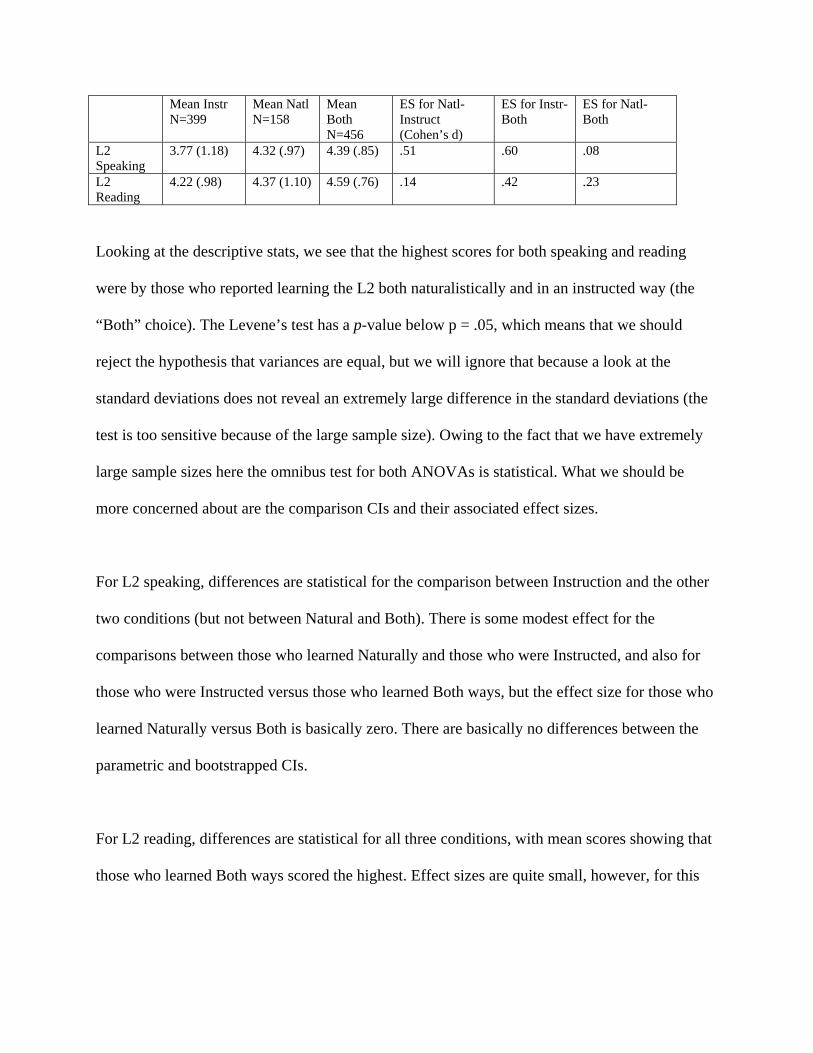
Mean Instr N=399
Mean Natl N=158
Mean Both N=456
ES for Natl-Instruct (Cohen’s d)
ES for Instr-Both
ES for Natl-Both
L2 Speaking
3.77 (1.18) 4.32 (.97) 4.39 (.85) .51 .60 .08
L2 Reading
4.22 (.98) 4.37 (1.10) 4.59 (.76) .14 .42 .23
Looking at the descriptive stats, we see that the highest scores for both speaking and reading
were by those who reported learning the L2 both naturalistically and in an instructed way (the
“Both” choice). The Levene’s test has a p-value below p = .05, which means that we should
reject the hypothesis that variances are equal, but we will ignore that because a look at the
standard deviations does not reveal an extremely large difference in the standard deviations (the
test is too sensitive because of the large sample size). Owing to the fact that we have extremely
large sample sizes here the omnibus test for both ANOVAs is statistical. What we should be
more concerned about are the comparison CIs and their associated effect sizes.
For L2 speaking, differences are statistical for the comparison between Instruction and the other
two conditions (but not between Natural and Both). There is some modest effect for the
comparisons between those who learned Naturally and those who were Instructed, and also for
those who were Instructed versus those who learned Both ways, but the effect size for those who
learned Naturally versus Both is basically zero. There are basically no differences between the
parametric and bootstrapped CIs.
For L2 reading, differences are statistical for all three conditions, with mean scores showing that
those who learned Both ways scored the highest. Effect sizes are quite small, however, for this

area and there aren’t very big differences between groups. There are also basically no differences
between the parametric and bootstrapped CIs.
6 Jensen & Vinther (2003)
Use the Jensen&Vinther2003.sav file. Import into R as jensen.
a.CheckAssumptionsWe assume that the variables were independently gathered. Use histograms as well as numerical
values for skewness and kurtosis to check on normality assumptions and homogeneity of
variances. See Exercise #1 and Exercise #4 for similar datasets. Since you have detailed
instructions in those exercises, I will only give bare bones instructions for this dataset.
SPSS Instructions:
In the EXPLORE option, put the variable of GAINSCOR in the “Dependent List”. Put GROUP in the
“Factor List.”
R Instructions:
Boxplot(gainscore~group, data=jensen, id.method="y")
with(jensen, Hist(gainscore, groups=group, scale="frequency",
breaks="Sturges", col="darkgray"))
Control group is in rows 1:20, FSF in rows 21:41, and FSS in rows 42:62.
basicStats(jensen$gainscore[1:20])
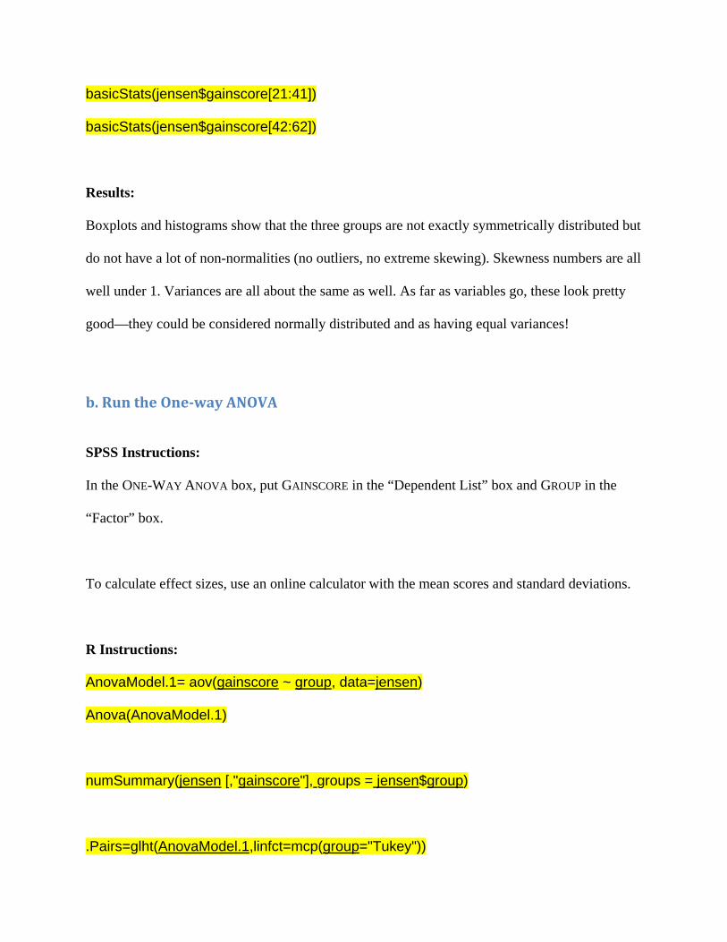
basicStats(jensen$gainscore[21:41])
basicStats(jensen$gainscore[42:62])
Results:
Boxplots and histograms show that the three groups are not exactly symmetrically distributed but
do not have a lot of non-normalities (no outliers, no extreme skewing). Skewness numbers are all
well under 1. Variances are all about the same as well. As far as variables go, these look pretty
good—they could be considered normally distributed and as having equal variances!
b.RuntheOne‐wayANOVA
SPSS Instructions:
In the ONE-WAY ANOVA box, put GAINSCORE in the “Dependent List” box and GROUP in the
“Factor” box.
To calculate effect sizes, use an online calculator with the mean scores and standard deviations.
R Instructions:
AnovaModel.1= aov(gainscore ~ group, data=jensen)
Anova(AnovaModel.1)
numSummary(jensen [,"gainscore"], groups = jensen$group)
.Pairs=glht(AnovaModel.1,linfct=mcp(group="Tukey"))

confint(.Pairs)
For a Bootstrapped One-way ANOVA
MeanDifference <- function (data,i){
temp<-data[i,]
aov.temp<-aov(gainscore ~ group, data=temp)
Tuk <-TukeyHSD(aov.temp)
return(Tuk$group[,1])
}
MeanDifferenceBoot <- boot(jensen, MeanDifference, 2000)
PAIRci.s <- NULL
PAIRt0 <- as.data.frame(MeanDifferenceBoot[1])
for(i in 1:length(MeanDifferenceBoot[[1]])){
CI <- boot.ci(MeanDifferenceBoot, conf = .95,
type = "bca", t0 = MeanDifferenceBoot$t0[i] ,
t = MeanDifferenceBoot$t[,i])
PAIRci.s[[paste("lwr",i,sep=".")]]<- CI$bca[c(4)]
PAIRci.s[[paste("upr",i,sep=".")]]<- CI$bca[c(5)]
}
Pci <- matrix(PAIRci.s, ncol = 2, nrow = length(PAIRt0[[1]]),
byrow=TRUE)

PAIRboot.ci <- data.frame(PAIRt0[1], lwr = Pci[, 1], upr = Pci[, 2])
print(PAIRboot.ci)
To calculate Cohen’s d effect size (and associated confidence intervals around this effect size),
the following code should work:
bootES(jensen, R=500, data.col="gainscore", group.col="group",
contrast=c(FSF=1,Control =-1),effect.type=c("cohens.d"), ci.type=c("bca"))
bootES(jensen, R=500, data.col="gainscore", group.col="group",
contrast=c(FSS=1,Control =-1),effect.type=c("cohens.d"), ci.type=c("bca"))
bootES(jensen, R=500, data.col="gainscore", group.col="group",
contrast=c(FSS=1,FSF =-1),effect.type=c("cohens.d"), ci.type=c("bca"))
Results:
Results from R
Omnibus F test
CI for mean difference FSF-Control
CI for mean difference FSS-Control
CI for mean difference FSS-FSF
Gainscore F2,59=5.20, p=.008
-.65, 59.01 7.89, 66.24 -21.58, 36.06
Bootstrapped CIs
7.12, 52.31 12.80, 60.34 -15.01, 31.11

Mean Control N=20
Mean FSF N=21
Mean FSS N=21
ES for FSF-Control (Cohen’s d)
ES for FSS-Control
ES for FSS-FSF
Gainscore 11.6 (38.75) 41.43 (37.37)
48.67 (40.36)
0.78 [.07, 1.38]
0.94 [.37, 1.60]
.19 [-.40, .83]
The mean scores show clearly that the control group fared far worse than either experimental
group. The parametric confidence interval for the difference between the FSF (fast-slow-fast)
group and the control, however, went through zero, although the lower level was quite close to
zero and with more precision would probably be farther away from zero. In fact, the
bootstrapped confidence interval did not go through zero and showed a minimum of about 7
points of difference in the CI, with up to 52 points of difference between the groups. So here is
one case where bootstrapping made quite a difference. The effect size estimate for this
comparison was fairly large, although the CI of the Cohen’s d effect size was also very wide and
shows that the estimate is not very precise. So we may hope and suspect there is a difference
between the control group and the FSF group, but there is some evidence for caution in making
that assumption!
There is clearly no difference between the FSS and FSF groups, with both the parametric and
bootstrapped CIs going through zero and the effect size being quite small, with a CI very close to
zero. On the other hand, there is a clear difference between the Control group and the FSS group,
although the CIs and confidence interval of the effect size shows it could be a fairly modest
effect.