Answers to problems sheet for PX384L - Electrodynamics · use cylindrical coordinates and the radial part of the divergence operator ... Verify using the Laplacian in spherical geometry

PX384L - Electrodynamics Answers to problem sheet

Answers to problems sheet for PX384L - Electrodynamicshttp://www.warwick.ac.uk/go/erwin verwichte/teaching/

Problem I.1Write the dimensions of all quantities in terms of the basic SI units of mass (kg), distance (m),time (s) and electric charge (C).

The basic SI units are mass (kg), length (m), time (s) and electric charge (C). All other units can bewritten as a combination of these basic units:

Quantity units in SI unitsForce ~F N (Newton) kg m s−2

Voltage U V (Volt) kg m2 s−2 C−1

Electric field ~E V/m or N/C kg m s−2 C−1

Magnetic induction ~B T (Tesla) kg s−1 C−1

Electric charge density ρ C/volume m−3CElectric current ~I A (Ampere) s−1 CElectric current density ~j A/surface area m−2 s−1 CPermittivity εo F/m (Farad/length) kg−1 m−3 s2 C2

Permeability µo H/m (Henry/length) kg m C−2

Conductivity σ S/m (Siemens/length) kg−1 m−3 s C2

Electric displacement ~D FV/m2 m−2 CElectric polarisation ~P FV/m2 m−2 CElectric dipole moment ~p FVm m CMagnetic field ~H Tm/H m−1 s−1 CMagnetisation ~M Tm/H m−1 s−1 CMagnetic dipole moment ~µ Tm4/H or Am2 m2 s−1 C

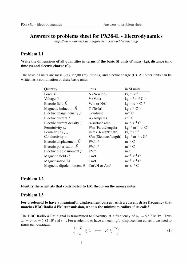
Problem I.2Identify the scientists that contributed to EM theory on the money notes.

Problem I.3For a solenoid to have a meaningful displacement current with a current drive frequency thatmatches BBC Radio 4 FM transmission, what is the minimum radius of its coils?

The BBC Radio 4 FM signal is transmitted to Coventry at a frequency of ν4 = 92.7 MHz. Thusω4 = 2πν4 = 5.82 108 rad s−1. For a solenoid to have a meaningful displacement current, we need tofulfill the condition

1

2

ω4R

co

& 1 ⇐⇒ R & 2co

ω4

(1)

1


The physicists that have contributed to electromagnetism and who have been immortalised on thebank notes.

Using co = 2.9979 108 m s−1, we find that R & 1.03 m.

Problem I.4Use the integral version of Gauss Law to find the electric field, ~E, electric displacement, ~D, andelectric polarisation, ~P , for a slab of dielelectric of relative permittivity εr which fills the spacebetween z = ±a and contains a uniform density of electric charges ρf per unit volume. Use theintegral version of ~∇. ~P = −ρp to find the surface density of polarisation charge on the surfaceof the dielectric.

The integral version of Gauss’ Law is

S

~D.d~S =y

V

ρfreedV (2)

The space between the plates is the volume V = S 2a. Gauss Law then becomes

D S = ρfree S 2a ⇒ D = ρfree 2a (3)

The electric displacement is oriented in the z-direction. The magnitudes of the electric field andpolarisation are given as

E =1

εrεo

D =ρfree 2a

εrεo

(4)

P = D − εo E = εo (εr − 1) E =

(1− 1

εr

)ρfree 2a (5)

In response to the electric field, the atoms in the dielectric will electrically polarise, such as to opposethe electric field. Because the atoms themselves are not mobile, the polarisation charge only manifestsitself at the surface of the dielectric. The amount of polarisation charges available together on bothsurfaces is (1 − ε−1

r )ρfree. Because an atom can only be near one of the edges, the surface charge onone surface is only half the available charge. Thus, for the volume in between the planes z = 0 and

2


z = a, a positive polarisation charge is present.

1

2

S

~P .d~S = −y

V

ρpoldV =x

S

σpoldS (6)

With ~P .d~S = PS, we find

1

2P S = σpol S ⇒ σpol =

1

2P =

(1− 1

εr

)ρfree a (7)

For the volume in between the planes z = −a and z = 0, a negative polarisation charge is present,which is equal to

σpol = −(

1− 1

εr

)ρfree a (8)

Problem I.5A steady beam of electrons has a radius R and a uniform charge density ρ = −ene. Outside thebeam there are no charges. Using Gauss Law, calculate the electric field for this system. For thisuse cylindrical coordinates and the radial part of the divergence operator (~∇. ~E)r = 1

r∂∂r

(rEr).Match the solutions inside and outside the beam at r = R.

Gauss’ Law is ~∇. ~E = ρ/εo. Because the charge density is uniform both in the beam as well as outside(trivially), the z and azimuthal ϕ components of the electric field will be constant or zero. We shall notconsider these components further. However, in the radial direction the charge density changes fromρ = −ene to ρ = 0. Therefore, we expect the radial component of the electric field to be non-constant.

In the particle beam, from 0 ≤ r ≤ R, Gauss’ Law becomes in cylindrical coordinates:

1

r

d

dr(rEr) =

ρ

εo

, (9)

which has the solutionEr(r) =

1

2

ρ

εo

r 0 ≤ r ≤ R (10)

Outside the particle beam, from R < r < ∞, Gauss’ Law reads:

1

r

d

dr(rEr) = 0 , (11)

which has the solutionEr(r) =

c

r, (12)

where c is an arbitrary constant.

3


The electric field is a continuous function. This means that the internal and external solutions mustmatch at r = R. Thus,

Er(R)internal = Er(R)external ⇔ 1

2

ρ

εo

R =c

R, (13)

from which we find the value of c:c =

1

2

ρ

εo

R2 (14)

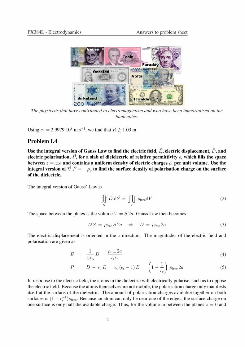
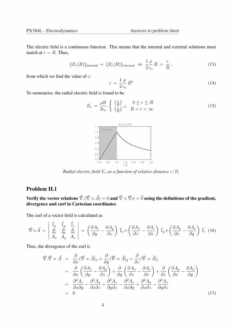
To summarise, the radial electric field is found to be

Er =ρR

2εo

.

(rR

)0 ≤ r ≤ R(

rR

)−1R < r < ∞ (15)

Radial electric field Er as a function of relative distance r/R.

Problem II.1Verify the vector relations ~∇.(~∇× ~A) = 0 and ~∇× ~∇φ = ~0 using the definitions of the gradient,divergence and curl in Cartesian coordinates

The curl of a vector field is calculated as

~∇× ~A =

∣∣∣∣∣∣

~1x~1y

~1z∂∂x

∂∂y

∂∂z

Ax Ay Az

∣∣∣∣∣∣=

(∂Az

∂y− ∂Ay

∂z

)~1x+

(∂Ax

∂z− ∂Az

∂x

)~1y+

(∂Ay

∂x− ∂Ax

∂y

)~1z (16)

Thus, the divergence of the curl is

~∇.~∇× ~A =∂

∂x(~∇× ~A)x +

∂

∂y(~∇× ~A)y +

∂

∂z(~∇× ~A)z

=∂

∂x

(∂Az

∂y− ∂Ay

∂z

)+

∂

∂y

(∂Ax

∂z− ∂Az

∂x

)+

∂

∂z

(∂Ay

∂x− ∂Ax

∂y

)

=∂2Az

∂x∂y− ∂2Ay

∂x∂z+

∂2Ax

∂y∂z− ∂2Az

∂x∂y+

∂2Ay

∂x∂z− ∂2Ax

∂y∂z= 0 (17)

4


Secondly, substituting ~∇φ = ∂φ∂x

~1x + ∂φ∂y

~1y + ∂φ∂z

~1z in place of ~A into the expression for curl of a vectorfield, we find:

~∇× ~∇φ =

(∂

∂y

∂φ

∂z− ∂

∂z

∂φ

∂y

)~1x +

(∂

∂z

∂φ

∂x− ∂

∂x

∂φ

∂z

)~1y +

(∂

∂x

∂φ

∂y− ∂

∂y

∂φ

∂x

)~1z

= ~0 (18)

Problem II.2Verify that the relations between the potentials and sources are also gauge invariant.

From Gauss’ Law, we have the Equation

~∇2φ +∂

∂t~∇. ~A = − ρ

εo

(19)

To show that this equation is gauge invariant, we substitute φ′, ~A′ for φ, ~A and using the gauge trans-form that the equation remains the same:

~∇2φ′ +∂

∂t~∇. ~A′ = − ρ

εo

⇔ ~∇2

(φ− ∂χ

∂t

)+

∂

∂t~∇.

(~A + ~∇χ

)= − ρ

εo

⇔ ~∇2φ +∂

∂t~∇. ~A− ~∇2∂χ

∂t+

∂

∂t~∇2χ = − ρ

εo

⇔ ~∇2φ +∂

∂t~∇. ~A = − ρ

εo

(20)

which proves the gauge invariance of the equation.From Ampere’s Law. we have the Equation

~∇2 ~A− 1

c2o

∂2 ~A

∂t2− ~∇

[~∇. ~A +

1

c2o

∂φ

∂t

]= −µo

~j (21)

We prove gauge invariance in the same way as before:

~∇2 ~A′ − 1

c2o

∂2 ~A′

∂t2− ~∇

[~∇. ~A′ +

1

c2o

∂φ′

∂t

]= −µo

~j

⇔ ~∇2(

~A + ~∇χ)− 1

c2o

∂2

∂t2

(~A + ~∇χ

)− ~∇

[~∇.

(~A + ~∇χ

)+

1

c2o

∂

∂t

(φ− ∂χ

∂t

)]= −µo

~j

⇔ ~∇2 ~A− 1

c2o

∂2 ~A

∂t2− ~∇

[~∇. ~A +

1

c2o

∂φ

∂t

]+ ~∇2~∇χ− 1

c2o

∂2

∂t2~∇χ− ~∇~∇2χ + ~∇ 1

c2o

∂2χ

∂t2= −µo

~j

⇔ ~∇2 ~A− 1

c2o

∂2 ~A

∂t2− ~∇

[~∇. ~A +

1

c2o

∂φ

∂t

]= −µo

~j (22)

5


Problem II.3Verify using the Laplacian in spherical geometry that the Laplacian of a potential function iszero.

A function f(~r) is potential if f(~r) = f0 r−1, where r is the radial coordinate and f0 is a constant. Apotential function is also harmonic. This means it obeys the relation ~∇2f = 0. To show this we writethe Laplacian in spherical coordinates:

~∇2f =1

r2

∂

∂r

(r2∂f

∂r

)+

1

r2 sin θ

∂

∂θ

(sin θ

∂f

∂θ

)+

1

r2 sin2 θ

∂2f

∂ϕ2(23)

For f = f0 r−1, we find

~∇2f =1

r2

∂

∂r

[r2 ∂

∂r

(f0

r

)]= −f0

1

r2

∂

∂r

[r2.

1

r2

]= −f0

1

r2

∂

∂r(1) = 0 (24)

Problem II.4Consider three immobile charges:a proton at (a, 0, 0), an electron at (−a/2,

√3a/2, 0) and an-

other electron at (−a/2,−√3a/2, 0).a) Plot and discuss this charge configuration.b) Write the electric charge density in terms of three contributions which each contain deltafunctions of the form qδ(x − x0)δ(y − y0)δ(z − z0) with r0 the charge location. Use f(x0) =∫ +∞−∞ f(x)δ(x− x0)dx.

c) Use the integral solution of Poisson’s equation to calculate the electrostatic potential for thischarge configuration.d) Calculate the corresponding electric field. We place a mobile electron at the origin. Writedown the equation of motion for this electron and calculate the acceleration of the electron. Inwhich direction is the electron moving?

a) The position vectors of the three charged particles are ~rA = a~1x, ~rB = −a2~1x +

√3a2

~1y and ~rC =

−a2~1x −

√3a2

~1y. If we calculate the magnitude of these position vectors, we see that

|~rA| = a , |~rB| =

√a2

4+

3a2

4= a , |~rC| =

√a2

4+

3a2

4= a (25)

for all three ions, it is the same value a. This means that all three ions ly on a circle in the xy-planewith centre at the origin and of radius a.

b) We write the electric charge density using delta functions:

ρ(~r) = e δ(~r − ~rA)− e δ(~r − ~rB)− e δ(~r − ~rC) , (26)

6


which is short for

ρ(~r) = e δ(x−a) δ(y) δ(z)− e δ(x+a/2) δ(y−√

3a/2) δ(z)− e δ(x+a/2) δ(y+√

3a/2) δ(z) (27)

c) The electric potential is then calculated using this charge density (Note the erratum):

φ(~r) =1

4πεo

y

V

ρ(~r′)|~r − ~r′| dV

=e

4πεo

[y

V

δ(~r′ − ~rA)

|~r − ~r′| dV −y

V

δ(~r′ − ~rB)

|~r − ~r′| dV −y

V

δ(~r′ − ~rC)

|~r − ~r′| dV

]

=e

4πεo

[1

|~r − ~rA| −1

|~r − ~rB| −1

|~r − ~rC|]

(28)

d) The corresponding electric field is found from

~E(~r) = −~∇φ(~r)

= − e

4πεo

~∇[

1

|~r − ~rA| −1

|~r − ~rB| −1

|~r − ~rC|]

=e

4πεo

[(~r − ~rA)

|~r − ~rA|3 −(~r − ~rB)

|~r − ~rB|3 −(~r − ~rC)

|~r − ~rC|3]

(29)

The equation of motion of an electron is given as med~ve

dt= −e ~E(~re(t)). The electron is placed at

the origin. There, the electron feels an acceleration

d~ve

dt= − e

me

~E(~0)

= − e2

4πεome

[(−~rA)

|~rA|3 − (−~rB)

|~rB|3 − (−~rC)

|~rC|3]

=e2

4πεome a3(~rA − ~rB − ~rC)

=e2

4πεome a32a~1x

=e2

2πεome a2~1x (30)

We can understand this result from using the Coulomb force formalism. The electron is repulsed bythe two negatively charged particles B and C, and is accelerated by them in the positive x-direction.The force the electron feels at the origin from ions B and C is equivalent to one negatively chargedparticle of charge −e placed at x=-a, y=0, z=0 (this equivalence is not true for other positions). Theacceleration the electron thus feels from ions B and C is e2/4πεoa

2. Furthermore, the electron isattracted to the positively charge particle A, and is accelerated by it in the positive x-direction. The

7


amount of acceleration is also e2/4πεoa2. Therefore, the total acceleration of the electron due to all

three ions is twice e2/4πεoa2.

Problem II.5A magnetic field points in the z-direction, and its magnitude is proportional to time, and in-dependent of position. Find the vector potential. Assuming that the electrostatic potential iszero, find the induced electric field. Prove by direct integration using a circular circuit, that theFaradays Law holds. Use

∮C

~E.d~ =∫ s2

s1

~E.(d~/ds)ds

We consider a magnetic field in the z-direction proportional to time, i.e. ~B = B0(t/t0)~1z. Themagnetic field is related to the magnetic vector potential ~A through ~B = ~∇× ~A. Writing this relationout in cylindrical coordinates and using the specific form of the magnetic field, we obtain

B0t

t0~1z =

1

r

∣∣∣∣∣∣

~1r r~1ϕ~1z

∂∂r

∂∂ϕ

∂∂z

Ar rAϕ Az

∣∣∣∣∣∣

=

(1

r

∂Az

∂ϕ− ∂Aϕ

∂z

)~1r +

(∂Ar

∂z− ∂Az

∂r

)~1ϕ +

(1

r

∂

∂r(rAϕ)− 1

r

∂Ar

∂ϕ

)~1z (31)

or

1

r

∂Az

∂ϕ− ∂Aϕ

∂z= 0

∂Ar

∂z− ∂Az

∂r= 0

1

r

∂

∂r(rAϕ)− 1

r

∂Ar

∂ϕ= B0

t

t0(32)

We can invoke symmetries in the problem to simplify the above relations. The problem looks thesame if we change of z or ϕ. Thus, ∂/∂z = ∂/∂ϕ = 0. Therefore, the previous set of equationsreduces to

∂Az

∂r= 0 and

1

r

∂

∂r(rAϕ) = B0

t

t0(33)

This means that Az is a constant and that the form of Ar is irrelevant to the problem. Therefore, wechoose Ar = Az = 0. Also, we solve the equation for Aϕ as

∂

∂r(rAϕ) = r B0

t

t0⇒ Aϕ(r) =

1

2r B0

t

t0+

c

r(34)

where c is a constant. Because at t = 0 there was no magnetic field, and hence no magnetic vectorpotential, we need to set c = 0.The induced electric field is given by ~E = −∂ ~A/∂t and is here equal to

~E = −1

2r

B0

t0~1ϕ (35)

8


The integral version of Faraday’s Law is∮

C

~E.d~ = − ∂

∂t

x

S

~B.d~S (36)

which for the given problem becomes

−1

2

B0

t0

∮

C

r~1ϕ.d~ = −B0

t0

x

S

~1z.d~S (37)

A circular path in the xy-plane can be defined in terms of a vector ~ parameterised in terms of theazimuthal angle ϕ: ~ = r cos ϕ~1x + r sin ϕ~1y + z~1z = r~1r + z~1z, where r and z are fixed. Note thatd~/dϕ = −r sin ϕ~1x + r cos ϕ~1y = r~1ϕ. Thus, we can write

∮

C

~E.d~ = −1

2

B0

t0r

∫ 2π

0

~1ϕ.d~

dϕdϕ = −1

2

B0

t0r2

∫ 2π

0

dϕ = −B0

t0πr2 (38)

Also, for the circular path,

−B0

t0

x

S

~1z.d~S = −B0

t0

∫ 2π

0

∫ r

0

~1z.~1z rdϕdr = −B0

t0πr2 (39)

Therefore, we have verified that Faraday’s Law is satisfied.

Problem II.6a) A straight wire carries a constant electric current I in the positive z-direction. Which E.M.gauge is applicable here? Use the integral version of Ampere’s Law to calculate the magneticfield generated by the electric current.b) Confirm that Ampere’s Law, as a differential equation for the vector potential ~A, is equal to~∇2 ~A = −µo

~j.c) Consider now two straight wires: wire A carries a constant electric current I in the positivez-direction and is located at x=a, y=0, z=0, wire B carries a constant electric current I in thenegative z-direction and is located at x=−a, y=0, z=0. Write down the current density for thisconfiguration using delta functions. Each contribution will contain delta functions of the formδ(x− x0)δ(y − y0) with (x0,y0,0) the location of the wire.d) Using the current density, calculate the vector potential on the line x=y=0.e) (hard) Write ~r± ≡ (x ∓ a)~1x + y~1y and calculate the magnetic vector potential for any po-sition in space close to the wire. Use the relation f(x0) =

∫ +∞−∞ d(z′ − z)/

√r2± + (z′ − z)2 =

2 lim(z′−z)→∞ ln |2(z′ − z)| − 2 ln(r±) for (z′ − z) À r±.d) Calculate the magnetic field from the magnetic vector potential. Use ~∇ × ln(r±)~1z = (~r± ×~1z)/r

2±. Sketch the magnetic field. What do magnetic field lines represent in terms of the vector

potential?

9


a) For a straight wire carrying a constant current I no time-variations occur. Therefore, the Coulombgauge is applicable. This means also that the displacement current may be neglected. Thus, theintegral version of Ampere’s Law is applicable:

∮

C

~B.d~ = µo I (40)

Choosing the circuit C to be a circle with centre a the origin, of radius r and in the xy-plane, we findeasily

B 2πr = I ⇔ B =µoI

2πr(41)

Here r represents the distance from the wire. Note that the magnetic field becomes infinite at r = 0.However, we cannot apply this formula there because in reality a wire has a finite width and thisneeds to be taken into account. The right-hand-rule for currents shows that the magnetic field is in thepositive azimuthal direction, i.e.

~B =µoI

2πr~1ϕ (42)

b) The vector potential ~A is defined as ~B = ~∇× ~A. Substituting this definition into Ampere’s Law,we find

~∇× ~∇× ~A = µo~j (43)

Using a vector identity, we can rewrite this as

~∇(~∇. ~A)− ~∇2 ~A = µo~j (44)

For the Coulomb gauge we assumed that ~∇. ~A = 0. Hence, we find

~∇2 ~A = −µo~j (45)

c) The current density from the two wires can be written using delta functions as

~j = I δ(x− a) δ(y)~1z − I δ(x + a) δ(y)~1z (46)

d) The vector potential is then calculated using this current density (Note the erratum):

~A(~r) =µo

4π

y

V

~j(~r′)|~r − ~r′| dV

=µoI

4π

[+∞y

−∞

δ(x− a) δ(y)

|~r − ~r′| dx′dy′dz′ −+∞y

−∞

δ(x + a) δ(y)

|~r − ~r′| dx′dy′dz′]

~1z

=µoI

4π

[+∞w

−∞

dz′√(x− a)2 + y2 + (z′ − z)2

−+∞w

−∞

dz′√(x + a)2 + y2 + (z′ − z)2

]~1z (47)

10


When we evaluate this expression on the z-axis, we find that

~A(0, 0, z) =µoI

4π

[+∞w

−∞

dz′√a2 + (z′ − z)2

−+∞w

−∞

dz′√a2 + (z′ − z)2

]~1z = ~0 (48)

The contributions from both wires cancel each other exactly.

e) We can calculate the vector potential for other positions. For this we continue the calculation fromEq. (47). We first introduce the notations

~rp = (x− a)~1x + y~1y , ~rm = (x + a)~1x + y~1y (49)

rp =√

(x− a)2 + y2 , rm =√

(x + a)2 + y2 (50)

rp and rm are the distances from the point of measurement to each of the two wires. Then:

~A(~r) =µoI

4π

∫ +∞

−∞

d(z′ − z)√r2p + (z′ − z)2

−∫ +∞

−∞

d(z′ − z)√r2m + (z′ − z)2

~1z (51)

We now use the tip that the following integral is equal to

+∞w

−∞

dx√k2 + x2

= 2

+∞w

0

dx√k2 + x2

= 2 limx→∞

ln |x +√

k2 + x2| − 2 ln |x +√

k2 + x2|(x = 0)

= 2 limx→∞

ln |2x| − 2 ln |k| (52)

In the last step, we used the approximation that for x À k,√

k2 + x2 ≈ x. This approximationbecomes precisely correct in the limit to infinity. We see that the first term actually is infinite. Usingthe previous result, the expression for the vector potential then becomes

~A(~r) =µoI

4π

[2 lim(z′−z)→∞

ln |2(z′ − z)| − 2 ln rp − 2 lim(z′−z)→∞

ln |2(z′ − z)| + 2 ln rm

]~1z

= −µoI

2π[ln rp − ln rm] ~1z

= −µoI

2π

[ln

√(x− a)2 + y2 − ln

√(x + a)2 + y2

]~1z (53)

The vector potential only depends on the x and y-coordinates, but not on the z-coordinate. Also,we see that the two infinite terms cancel each other exactly. Therefore, the vector potential remainsfinite everywhere, except at the position of the wires themselves where one of the two other termswill becomes infinite. However, it is unphysical to apply this expression there because in reality awire has a finite width and if this is taken into account, the infinity is removed. For the case of oneinfinite wire, as studied in part a), the vector potential is in fact infinite. But this infinity is removedwhen calculating the magnetic field because the term responsible for the infinity does not depend on

11


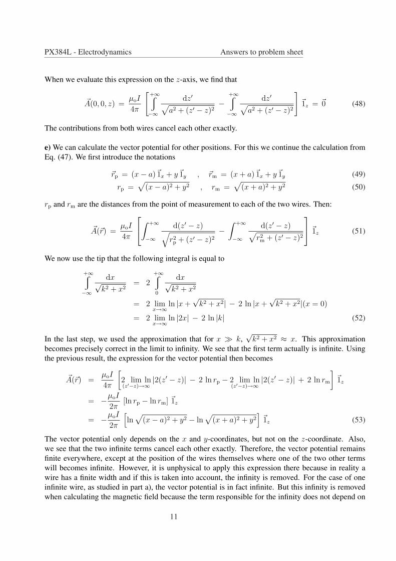
Contours of constant Az as a function of x and y for two straight opposite current-carrying wires.The magnetic fieldlines correspond to the contours of constant Az.

the radial coordinate away from the wire, and therefore does not contribute to ~∇× Az~1z.

f) The magnetic field is given in function of the vector potential as ~B = ~∇× ~A. Using that d ln f(x)dx

=df(x)

dx/x, ∂rp

∂y= y/rp, ∂rp

∂x= (x − a)/rp, ∂rm

∂y= y/rm and ∂rm

∂x= (x + a)/rm, we then find that

~∇× ln rp~1z = (~rp ×~1z)/r

2p. Thus the magnetic field vector becomes

~B = −µoI

2π

[(~rp ×~1z)

r2p

− (~rm ×~1z)

r2m

](54)

At the z-axis, the magnetic fields of the two wires add up to double their individual contribution.Because x=y=0, then ~rp = −a~1x and ~rm = a~1x. Thus, Eq. (54) is at the z-axis equal to

~B(0, 0, z) = −µoI

πa~1y (55)

We interpret the magnetic field in Eq. (54) as the superposition of the magnetic field of two wires,with each wire shifted from the origin. Indeed, the magnetic field from a single wire along the z-axiscan be written as

~B = −µoI

2π

(~r ×~1z)

r2=

µoI

2πr~1ϕ (56)

which confirms the result found in part a). For the one wire case, we see that a magnetic fieldline hasthe shape of a circular curve in the xy-plane. Thus, for all points on a specific fieldline, the distance r

12


is the same. This then implies that for all those points the z-component of the vector potential Az hasthe same value. Therefore, on a magnetic field line, the vector potential is constant! This conclusionalso applies for the case of the two wires (see Figure).

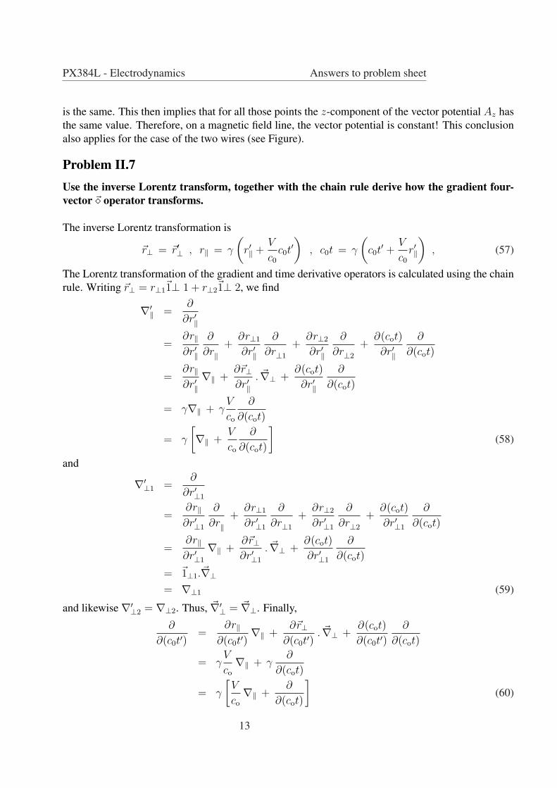
Problem II.7Use the inverse Lorentz transform, together with the chain rule derive how the gradient four-vector ~¦ operator transforms.

The inverse Lorentz transformation is

~r⊥ = ~r′⊥ , r‖ = γ

(r′‖ +

V

c0

c0t′)

, c0t = γ

(c0t

′ +V

c0

r′‖

), (57)

The Lorentz transformation of the gradient and time derivative operators is calculated using the chainrule. Writing ~r⊥ = r⊥1

~1⊥ 1 + r⊥2~1⊥ 2, we find

∇′‖ =

∂

∂r′‖

=∂r‖∂r′‖

∂

∂r‖+

∂r⊥1

∂r′‖

∂

∂r⊥1

+∂r⊥2

∂r′‖

∂

∂r⊥2

+∂(cot)

∂r′‖

∂

∂(cot)

=∂r‖∂r′‖

∇‖ +∂~r⊥∂r′‖

. ~∇⊥ +∂(cot)

∂r′‖

∂

∂(cot)

= γ∇‖ + γV

co

∂

∂(cot)

= γ

[∇‖ +

V

co

∂

∂(cot)

](58)

and

∇′⊥1 =

∂

∂r′⊥1

=∂r‖∂r′⊥1

∂

∂r‖+

∂r⊥1

∂r′⊥1

∂

∂r⊥1

+∂r⊥2

∂r′⊥1

∂

∂r⊥2

+∂(cot)

∂r′⊥1

∂

∂(cot)

=∂r‖∂r′⊥1

∇‖ +∂~r⊥∂r′⊥1

. ~∇⊥ +∂(cot)

∂r′⊥1

∂

∂(cot)

= ~1⊥1.~∇⊥= ∇⊥1 (59)

and likewise ∇′⊥2 = ∇⊥2. Thus, ~∇′

⊥ = ~∇⊥. Finally,

∂

∂(c0t′)=

∂r‖∂(c0t′)

∇‖ +∂~r⊥

∂(c0t′). ~∇⊥ +

∂(cot)

∂(c0t′)∂

∂(cot)

= γV

co

∇‖ + γ∂

∂(cot)

= γ

[V

co

∇‖ +∂

∂(cot)

](60)

13


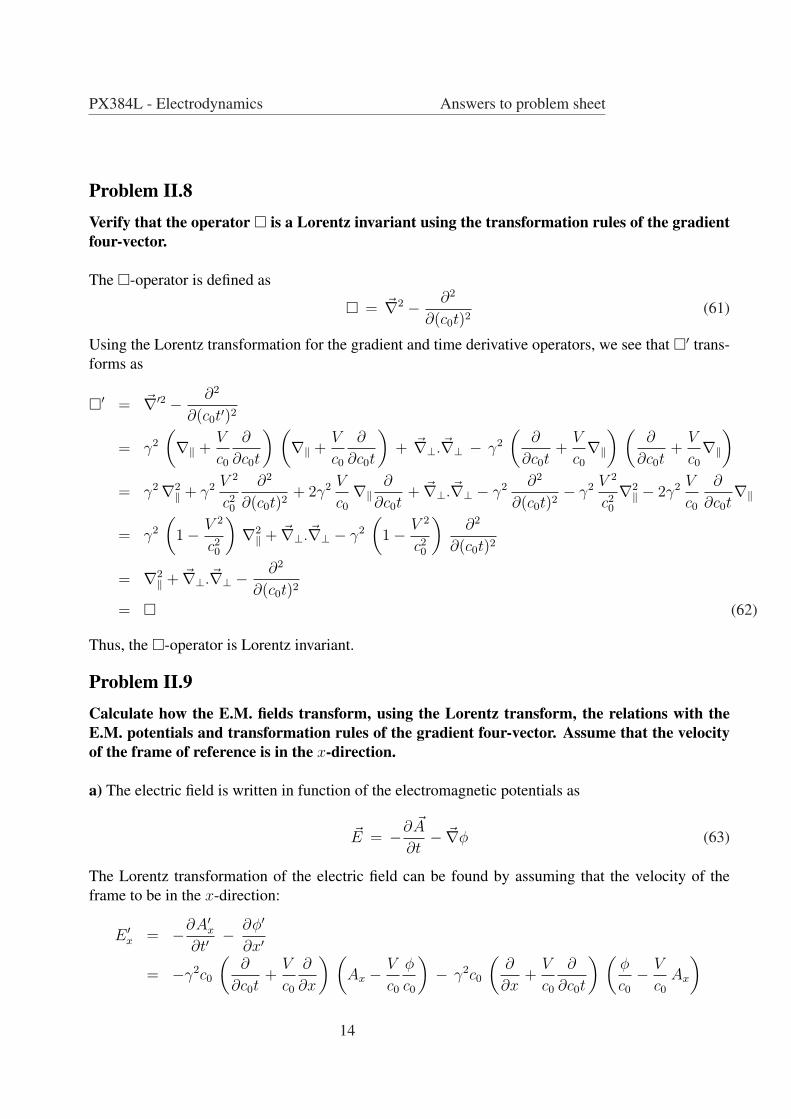
Problem II.8Verify that the operator ¤ is a Lorentz invariant using the transformation rules of the gradientfour-vector.

The ¤-operator is defined as

¤ = ~∇2 − ∂2

∂(c0t)2(61)

Using the Lorentz transformation for the gradient and time derivative operators, we see that ¤′ trans-forms as

¤′ = ~∇′2 − ∂2

∂(c0t′)2

= γ2

(∇‖ +

V

c0

∂

∂c0t

) (∇‖ +

V

c0

∂

∂c0t

)+ ~∇⊥.~∇⊥ − γ2

(∂

∂c0t+

V

c0

∇‖

) (∂

∂c0t+

V

c0

∇‖

)

= γ2∇2‖ + γ2 V 2

c20

∂2

∂(c0t)2+ 2γ2 V

c0

∇‖∂

∂c0t+ ~∇⊥.~∇⊥ − γ2 ∂2

∂(c0t)2− γ2 V 2

c20

∇2‖ − 2γ2 V

c0

∂

∂c0t∇‖

= γ2

(1− V 2

c20

)∇2‖ + ~∇⊥.~∇⊥ − γ2

(1− V 2

c20

)∂2

∂(c0t)2

= ∇2‖ + ~∇⊥.~∇⊥ − ∂2

∂(c0t)2

= ¤ (62)

Thus, the ¤-operator is Lorentz invariant.

Problem II.9Calculate how the E.M. fields transform, using the Lorentz transform, the relations with theE.M. potentials and transformation rules of the gradient four-vector. Assume that the velocityof the frame of reference is in the x-direction.

a) The electric field is written in function of the electromagnetic potentials as

~E = −∂ ~A

∂t− ~∇φ (63)

The Lorentz transformation of the electric field can be found by assuming that the velocity of theframe to be in the x-direction:

E ′x = −∂A′

x

∂t′− ∂φ′

∂x′

= −γ2c0

(∂

∂c0t+

V

c0

∂

∂x

) (Ax − V

c0

φ

c0

)− γ2c0

(∂

∂x+

V

c0

∂

∂c0t

) (φ

c0

− V

c0

Ax

)

14


= −γ2c0

(1− V 2

c20

)∂Ax

∂c0t− γ2c0

(1− V 2

c20

)∂

∂x

(φ

c0

)

− γ2c0

[−V

c0

∂

∂c0t

(φ

c0

)+

V

c0

∂Ax

∂x− V

c0

∂ Ax

∂x+

V

c0

∂

∂c0t

(φ

c0

)]

= −γ2c0

(1− V 2

c20

) [∂Ax

∂c0t+

∂

∂x

(φ

c0

)]

= −∂Ax

∂t− ∂φ

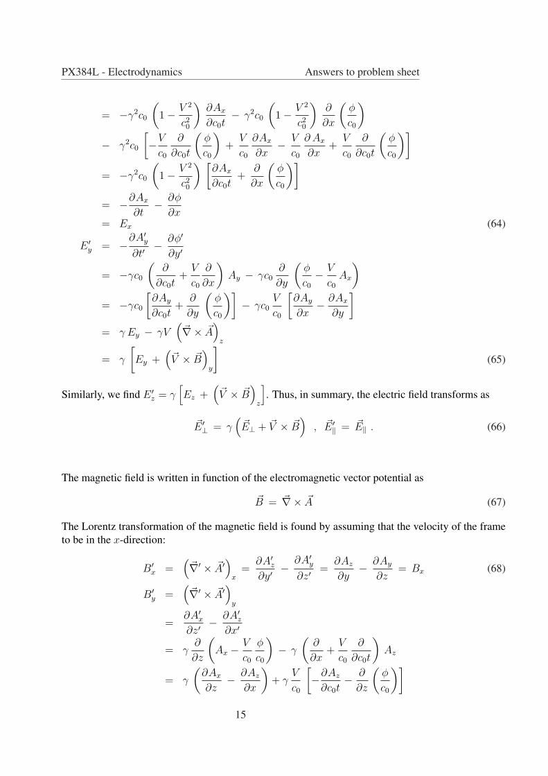
∂x= Ex (64)

E ′y = −∂A′

y

∂t′− ∂φ′

∂y′

= −γc0

(∂

∂c0t+

V

c0

∂

∂x

)Ay − γc0

∂

∂y

(φ

c0

− V

c0

Ax

)

= −γc0

[∂Ay

∂c0t+

∂

∂y

(φ

c0

)]− γc0

V

c0

[∂Ay

∂x− ∂Ax

∂y

]

= γ Ey − γV(

~∇× ~A)

z

= γ

[Ey +

(~V × ~B

)y

](65)

Similarly, we find E ′z = γ

[Ez +

(~V × ~B

)z

]. Thus, in summary, the electric field transforms as

~E ′⊥ = γ

(~E⊥ + ~V × ~B

), ~E ′

‖ = ~E‖ . (66)

The magnetic field is written in function of the electromagnetic vector potential as

~B = ~∇× ~A (67)

The Lorentz transformation of the magnetic field is found by assuming that the velocity of the frameto be in the x-direction:

B′x =

(~∇′ × ~A′

)x

=∂A′

z

∂y′− ∂A′

y

∂z′=

∂Az

∂y− ∂Ay

∂z= Bx (68)

B′y =

(~∇′ × ~A′

)y

=∂A′

x

∂z′− ∂A′

z

∂x′

= γ∂

∂z

(Ax − V

c0

φ

c0

)− γ

(∂

∂x+

V

c0

∂

∂c0t

)Az

= γ

(∂Ax

∂z− ∂Az

∂x

)+ γ

V

c0

[−∂Az

∂c0t− ∂

∂z

(φ

c0

)]

15


= γ By + γV Ez

c20

= γ

By − 1

c0

(~V ×

~E

c0

)

y

(69)

Similarly, we find B′z = γ

[Bz − 1

c0

(~V × ~E

c0

)z

]. Thus, in summary, the magnetic field transforms as

~B′⊥ = γ

(~B⊥ − 1

c0

~V ×~E

c0

), ~B′

‖ = ~B‖ . (70)

Problem III.1A particle with charge q is emitted from the origin with momentum p directed at an angle θ toa uniform magnetic field B which lies in the z-direction. At what point does the particle nextintersects the z-axis.

At time t = 0, the charge is at the origin with an initial velocity ~v(0) = (sin θ, 0, cos θ) pm

. Withoutloss of generality, the frame of reference has been chosen such that the initial velocity is in the xz-plane. The equation of motion for the particle of mass m and charge q in a uniform magnetic field inthe z-direction is

md~v

dt= qB~v ×~1z (71)

For this case, we have seen in the lectures that the parallel and perpendicular speeds remain constant.Thus, v⊥ = p

msin θ and v‖ = p

mcos θ. The equation of motion has the solution

vx(t) = pm

sin θ cos(Ωt + φ)vy(t) = −s p

msin θ sin(Ωt + φ)

vz(t) = pm

cos θ(72)

with s = q/|q| and Ω = |q|B/m. Integrating the previous equation in time gives the position of thecharge as a function of time:

x(t) = x0 + pΩm

sin θ sin(Ωt + φ)y(t) = y0 + s p

Ωmsin θ cos(Ωt + φ)

z(t) = z0 + pm

cos θ t(73)

The constants x0, y0, z0 and φ are determined from the initial conditions and we take x0 = 0, y0 =−s p

Ωmcos θ, z0 = 0 and φ = 0. Thus,

x(t) = pΩm

sin θ sin(Ωt)y(t) = s p

Ωmsin θ [cos(Ωt)− 1]

z(t) = pm

cos θ t(74)

We see examining the previous expressions that at t = 0 the particle is indeed at the origin. Thecharged particle crosses the z-axis if x(t) = y(t) = 0. Using the previous expression, we see that

16


x(t) = 0 when t = nπ/Ω with n an integer. y(t) = 0 if t = 2n′π/Ω with n′ another integer. The firsttime after t = 0 when both x(t) and y(t) become zero is when n = 2 and n′ = 1. Thus, t = 2π/Ω.This time corresponds to one gyro-period after the initial condition. In fact, at every time which ismultiple of the gyro-period, the charged particle crosses the z-axis.

Problem III.2The Earth’s magnetic field is to first approximation a dipole and we neglect the difference inorientation of the magnetic and rotation axis. A magnetic field line lies in a plane of constantEarth longitude, is of circular shape and goes through the centre of the Earth. We consider theequatorial plane. The dipolar magnetic field is there given by the formula B(r) = µo

4πMr3 , where

M is the magnitude of the magnetic moment. Near the Earth poles, the magnetic field strengthB0= 5 10−5 T. Note also that the Earth radius is about RE=6380 km. The Earth is surroundedby two radiation belts, known as the Van Allen belts, named after the Prof. James Van Allen,chief scientist of the first American satellites which discovered them. The charged particles thatpopulate these belts gyrate around and travel along the magnetic field lines and bounce backand forth between the poles. The inner and outer belts ly at 1.3 RE and 4 RE, respectively. Thehigh energy particles found in these belts can readily penetrate space crafts and are therefore ano go area for astronauts. The energy of such particles is often described in units of eV. 1 eV isequivalent to 1.6022 10−19 J.

a) We eliminate the magnetic moment from the formula of the magnetic dipole:

M =4π

µo

B(r)r3 , (75)

and use the fact that at r = RE, B(RE) = B0. Thus,

M =4π

4π10−75 10−5 (6380000)3 = 1.3 1023 A m2 . (76)

b) As seen in the previous question, we can write:

B0 =µo

4π

M

R3E

orµo

4πM = B0 R3

E . (77)

Substituting this into the formula of the dipole magnetic field:

B(r) = B0R3

E

r3= B0

(r

RE

)−3

. (78)

c) The gyro frequency is defined as Ω = |q|B/m. For a dipole magnetic field it is equal to

Ω =|q|B0

m

(r

RE

)−3

= Ω0

(r

RE

)−3

, (79)

17


with Ω0 = |q|B0/m. Thus, for electrons and protons

Ωe = Ω0e

(r

RE

)−3

, Ωp = Ω0p

(r

RE

)−3

, (80)

with Ω0e = 8.8 106 rad/s and Ω0e = 4800 rad/s. The Larmor radius is defined as rL = v⊥/Ω. Using theassumption that v⊥ = v/2, we write:

rL =v

2Ω=

mv

2|q|B =mv

2|q|B0

(r

RE

)3

. (81)

We write the particle speed v in function of the particle energy W = mv2/2 as

W =1

2m(mv)2 ⇒ mv =

√2mW , (82)

The expression for the Larmor radius is then rewritten as

rL =

√mW

2

1

|q|B0

(r

RE

)3

= rL0

(W

W0

)1/2 (r

RE

)3

, (83)

where W0 is the energy corresponding to 1 eV, which is 1.6022 10−19 J. Also, rL0 =√

mW0

21

|q|B0.

Thus, for electrons and protons

rLe = rL0e

(W

W0

)1/2 (r

RE

)3

, rLp = rL0p

(W

W0

)1/2 (r

RE

)3

(84)

with rL0e = 0.03 m and rL0p = 1.5 m.

d) The particles gyrate around the magnetic field in a helical orbit of radius rL. In the equatorial plane,the particle’s guiding centre (location of magnetic field line) is a distance r from the Earth’s centre,and thus a distance r − RE from the Earth surface. Because the thickness of the Earth atmosphere isvery small compared with the radius of the Earth, we neglect this and keep r − RE to represent thedistance from the particle’s guiding centre to the Earth atmosphere. The particle does not enter theEarth atmosphere if

rL < r −RE

⇒ rL0

(W

W0

)1/2 (r

RE

)3

< r −RE

⇔(

W

W0

)1/2

<r −RE

rL0

(r

RE

)−3

⇒(

W

W0

)<

(r −RE

rL0

)2 (r

RE

)−6

, (85)

which defined a maximum energy Wmax as

Wmax = W0

(r −RE

rL0

)2 (r

RE

)−6

. (86)

18


For the inner belt at r = 1.3 RE, we find for electrons and protons:

Wmax,e =

((1.3− 1)6380000

0.03

)2

(1.3)−6 = 6.7 1014 eV = 670 TeV , (87)

Wmax,p =

((1.3− 1)6380000

1.5

)2

(1.3)−6 = 3.6 1011 eV = 360 GeV . (88)

Similar for the outer belt at r = 4 RE, we find Wmax,e = 79 TeV and Wmax,p = 43 GeV. The protons inthe outer belt are of greatest risk of hitting the Earth atmosphere because its maximum energy is thelowest. Although this calculation is only a crude approximation, it does hint to the reality where theouter belt is mostly populated by high energy electrons, not protons.

e) Because of the dependence of the magnetic field on r and the curvature of the field lines, theparticles will drift. The drift velocity is given by

~vD =(

~FgradB + ~Fcurv

)×

~B

qB2

=

(−W⊥

~∇B

B− 2W‖

~1n

Rc

)×

~B

qB2, (89)

with particle energy perpendicular and parallel to the magnetic field W⊥ = mv2⊥/2 = W/4, W‖ =

mv2‖/2 = W/4. Also, ~1n is the unit vector directed to the centre of curvature at r/2 and is equal to

−~1r. Rc is the radius of curvature and because the magnetic field line is a circle of radius r/2, it isequal to Rc = r/2. The gradient of the magnetic field is calculated as

~∇B(r) = B0R3E

d

dr

(r−3

)~1r = −3 B0R

3E r−4~1r = −3

rB(r)~1r . (90)

Thus, the drift velocity is equal to

~vD =

(−W

4

(−3)

r~1r − 2

W

4

(−2)

r~1r

)×

~B

qB2

=7

4

W

r~1r ×

~B

qB2

= −7

4

W

qBr~1φ

= −7

4

W

qB0RE

(r

RE

)2

~1φ . (91)

We have used the fact that the Earth magnetic field points from the South to the North pole and at theequatorial plane is vertical. Thus, ~1r × ~B/B = ~1r × ~1z = −~1φ with ~1φ the azimuthal unit vector,directed anti-clockwise around the Earth when seen from the North pole.By defining vD0 = 7

4W0

|q|B0RE, we rewrite the drift velocity as

~vD = −vD0

(q

|q|) (

W

W0

) (r

RE

)2

~1φ . (92)

19


Again, for electrons and protons

~vDe = vD0e

(W

W0

) (r

RE

)2

~1φ ,

~vDp = −vD0p

(W

W0

) (r

RE

)2

~1φ , (93)

with vD0e = vD0p = 0.003 m/s.We see now that electrons drift around the Earth in the anti-clockwise direction as seen from the Northpole. The protons drift in the clockwise direction. Because the two particle species drift in oppositedirections, charge separation occurs and an electric current flows.The time for a particle to complete one rotation around the Earth is the trajectory distance 2πr dividedby the drift speed vD:

P =2πr

vD

=2πRE

vD

(r

RE

)=

2πRE

vD0

(W

W0

)−1 (r

RE

)−1

= P0

(W

W0

)−1 (r

RE

)−1

. (94)

with P0 = 2πRE

vD0which for electrons and protons alike is P0e = P0p = 1.3 1010 s≈ 400 yr. For particles

in the outer belt, r = 4 RE with energy W = 100 keV = 105 W0, we find P = 32000 s ≈ 9 hr. Forenergy W = 100 MeV = 108 W0, we find P = 32 s.

f) The electric current density is defined as

~j = −ene~vDe + enp~vDp = en (~vDp − ~vDe) , (95)

Using the previously derived expression for the drift velocity of electrons and protons we find

~j = −2 en vD0e

(W

W0

) (r

RE

)2

~1φ . (96)

For a number density n = 1010 m−3, the strength of the current in the outer belt is for particles ofenergy W = 100 keV = 105 W0 equal to j = 16 µA m−2 and for particles of energy W = 100 MeV =108 W0 equal to j = 16 mA m−2.

Problem IV.1Calculate the electron and proton plasma frequencies, Debye length, thermal speeds and gy-rofrequencies for the examples given on page 14. Use the plasma calculator on the modulewebpage at http://www.warwick.ac.uk/go/erwin verwichte/teaching/px384l/.//We use the following formula:

ωp,e =

√nee2

εome

, λD =

√εokBTe

nee2, Vth,e =

√kBTe

me

= λD ωp,e (97)

Ωe,p =eB

me,p, rL,e,p =

Vth,e

Ωe,p(98)

20


to calculate

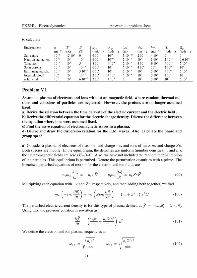
Environment n T B ωpe ωpp λD VTe VTp Ωe Ωp

(m−3) (K) (T) (rads−1) (rads−1) (m) (ms−1) (ms−1) (rads−1) (rads−1)Sun centre 1032 15 106 0 6 1017 1016 3 10−11 2 107 4 105 0 0Neutron star atmos. 1020 107 108 6 1011 1010 2 10−5 107 3 105 2 1019 9.6 1015

Tokamak 1019 108 5 8 1011 4 109 2 10−4 4 107 9 105 9 1011 5 108

Solar corona 1014 106 10−2 6 108 107 7 10−3 4 106 105 2 109 106

Earth magnetosph. 1010 103 5 10−5 6 106 105 2 10−2 105 3 103 9 106 5 103

Interstel. cloud 109 10 10−7 2 106 4 104 7 10−3 105 3 102 2 104 10solar wind 107 105 6 10−6 2 105 4 103 7 106 3 104 106 6 102

Problem V.1Assume a plasma of electrons and ions without an magnetic field, where random thermal mo-tions and colissions of particles are neglected. However, the protons are no longer assumedfixed.a) Derive the relation between the time derivate of the electric current and the electric field .b) Derive the differential equation for the electric charge density. Discuss the difference betweenthe equation where ions were assumed fixed.c) Find the wave equation of electromagnetic waves in a plasma.d) Derive and draw the dispersion relation for the E.M. waves. Also, calculate the phase andgroup speed.

a) Consider a plasma of electrons of mass me and charge −e, and ions of mass mi and charge Ze.Both species are mobile. In the equilibrium, the densities are uniform (number densities ne and ni),the electromagnetic fields are zero ( ~E= ~B=0). Also, we have not included the random thermal motionof the particles. This equilibrium is perturbed. Denote the perturbation quantities with a prime. Thelinearised perturbed equations of motion for the electron and ion fluids are

neme∂~u′e∂t

= −ne e ~E ′ , nimi∂~u′i∂t

= ni Ze~E ′ (99)

Multiplying each equation with −e and Ze, respectively, and then adding both together, we find

me

(−ene

∂~u′e∂t

)+ mi

(Zeni

∂~u′i∂t

)=

(ne + Z2ni

)e2 ~E ′ (100)

The perturbed electric current density is for this type of plasma defined as ~j′ = −ene~u′e + Zeni~u

′i.

Using this, the previous equation is rewritten as

∂~j′

∂t=

(nee

2

me

+niZ

2e2

mi

)~E ′ (101)

We define the electron and ion plasma frequencies as

ωp,e =

√nee2

meεo

, ωp,i =

√niZ2e2

miεo

(102)

21


Thus, after substituting these definitions into the equation for the current density, we find

∂~j′

∂t=

(ω2

p,e + ω2p,i

)εo

~E ′ = ω2p εo

~E ′ (103)

Here, a combined plasma frequency has been defined as

ωp =√

ω2p,e + ω2

p,i (104)

b) This is simple. We repeat the calculation as done for fixed ions, but replace the electron plasmafrequency everywhere with the combined plasma frequency. We take the divergence of the previousequation for the current density:

∂ ~∇.~j′

∂t= ω2

p εo~∇. ~E ′ (105)

We consider the linearised perturbed equations of charge conservation, ∂ρ′∂t

+ ~∇.~j′ = 0, and GaussLaw, ~∇. ~E ′ = ρ′/εo to rewrite the expression in terms of the perturbed charge density

−∂2ρ′

∂t2= ω2

p ρ′ (106)

or [∂2

∂t2+ ω2

p

]ρ′ = 0 (107)

This is an equation describing harmonic oscillations in charge density. We consider that the pertur-bation charge density is of the form ρ′(~r, t) =

∫ +∞−∞ ρ(~r, ω) e−iωt dω. Then, the equation reduces for

each component ρ(~r, ω) to (ω2 − ω2

p

)ρ = 0 (108)

This algebraic equation has two possible solutions,

ω2 6= ω2p , ρ = 0 electromagnetic waves in a plasma

ω2 = ω2p , ρ 6= 0 electrostatic plasma oscillations

(109)

Instead of the plasma frequency of electrons, it is this combined plasma frequency which involvedboth electron and ion frequency that determines the behaviour of the perturbation. Because the elec-tron is at least 1800 times lighter than the ion, and using quasi–neutrality to write Zni = ne, we seethat the combined plasma frequency is only slightly larger than the electron plasma frequency.

c) Again, we repeat the calculation as done for fixed ions, but replace the electron plasma frequencyeverywhere with the combined plasma frequency. Taking the divergence of Faradays Law, we findfor perturbed electromagnetic fields:

~∇×(

~∇× ~E ′)

= −~∇× ∂ ~B′

∂t(110)

Applying a vector identity to the left-hand side:

~∇(

~∇. ~E ′)− ~∇2 ~E ′ = − ∂

∂t~∇× ~B′ (111)

22


Using Gauss Law and Ampere’s Law:

~∇(

ρ′

εo

)− ~∇2 ~E ′ = −µo

∂~j′

∂t− µoεo

∂2 ~E ′

∂t2(112)

For electromagnetic waves in a plasma, the electric charge density is zero, ρ′ = 0. Also, using theexpression for the perturbed electric charge density, we find

−~∇2 ~E ′ = −µoεo ω2p

~E ′ − µoεo∂2 ~E ′

∂t2(113)

Lastly, using the definition for the speed of light in free space,[~∇2 − 1

c20

∂2

∂t2− ω2

p

c20

]~E = ~0 (114)

In a similar fashion, the electromagnetic wave equation in a plasma for the perturbed magnetic fieldis found to be [

~∇2 − 1

c20

∂2

∂t2− ω2

p

c20

]~B = ~0 (115)

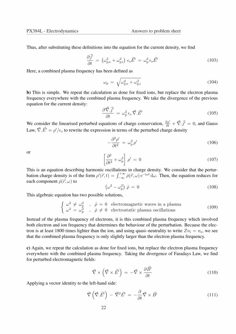
Dispersion diagram for electromagnetic waves in a plasma. Dashed line: dispersion relation for anelectromagnetic wave in free space..

d) We take the perturbed electromagnetic fields to have the form of a superposition of plane waves,i.e.

~E ′(~r, t) =x +∞x

−∞

~E(~k, ω) ei(~k.~r−ωt) dkxdkydkzdω (116)

23


where ~k and ω are the wave vector and wave frequency, respectively. The wave equation becomes for

a single component ~E(~k, ω)

[−k2 +

ω2

c20

− ω2p

c20

]~E(~k, ω) = ~0 (117)

For a wave of finite amplitude, i.e. ~E(~k, ω) 6= ~0, the wave fulfils the dispersion relation

ω2 = ω2p + c2

0 k2 (118)

The difference of this dispersion relation with the one for fixed ions again lies in the fact that theelectron plasma frequency has been replaced by the combined plasma frequency. Rewriting the dis-persion relation as k =

√ω2 − ω2

p/c0, we see there are two regimes of behaviour for electromagneticwaves in a plasma:

ω2 > ω2p k is real propagating wave

ω2 < ω2p k is imaginary damped wave

(119)

For propagating electromagnetic waves, we calculate the phase and group speeds:

Vph =ω

k=

ωc0√ω2 − ω2

p

=c0√

1− ω2p

ω2

(120)

Vg =∂ω

∂k=

∂

∂k

√ω2

p + c0 k2 =c20k

ω=

c20

Vph

= c0

√1− ω2

p

ω2(121)

Problem V.2Using spherical polar coordinates, verify that ~E = ~E0

f(r−c0t)r

represents a spherical electro-magnetic wave emanating from the origin. Calculate the wave energy density and show that thetotal wave energy is conserved as the wave spreads out.a) The Sun radiates electromagnetic waves corresponding to a black body at temperature of6000 K. Use Stefan’s Law P = σST

4A to calculate the total E.M. power output P , where σS =5.67 10−8 Wm−2K−4 is Stefan’s constant and A is the area through which the E.M. wave travels.The solar radius is 696000 km.b) Calculate the solar power per square meter, known as the solar constant, received at Earth,which is 150 million km away from the Sun. Also, calculate the amplitudes of the electric andmagnetic fields.c) Repeat the calculation for a star similar to the Sun which is located 10 light years from Earth.d) Repeat the calculation for a 5 W laser focused on a 1 µm spot. Compare and discuss the val-ues you found in parts b,c and d.

The wave energy density is given by

u =1

2εo E2 +

1

2µo

B2 = εo E2 =εo E2

0

r2|f(r − c0t)|2 (122)

24


The total wave energy over a sphere of radius r and surface area A is

U =

A

u dA = 4πr2 εo E20

r2|f(r − c0t)|2 = 4πεo E2

0 |f(r − c0t)|2 (123)

The function f does not depend on r in a way that would make the total energy increase or decrease(e.g. a plane wave f(r − c0t) = exp[i(kr − ωt)]). Thus, the total wave energy remains constant overa spherical surface. As wave energy in conserved in free space (no Joule heating for example), thismeans that the wave energy is spread out over the surface. As the wave expands from the centre andthe sphere grows in size, the wave energy density decreases as 1/r2, as the sphere surface grows as r2.

a) For the photospheric temperature of T¯=6000 K and solar radius R¯=6.96 108 m, the total E.Mpower from the Sun is equivalent to the P =

vA

∂u∂t

dA. Using Stefan’s Law:

P¯ = σS T 4¯ 4πR2

¯ = 4.47 1026 W (124)

b) The power received at the Earth per square meter is equal to the Poynting flux through the sphereof radius D⊕, where D⊕=1.5 1011 m is the mean Sun-Earth distance. Thus, the solar constant is

S⊕ =P¯

4πD⊕≈ 1600 W/m2 (125)

From the definition of the Poynting vector we know that S=| ~E × ~B|/µo= 1c0µo

E20= c0

µoB2

0 . Therefore,the electric and magnetic field amplitudes are

E0 =√

c0µo S⊕ = 780 V/m (126)

B0 =E0

c0

= 2.60 µT (127)

c) The solar power received per square meter at a star 10 light years is equal to the Poynting fluxthrough the sphere of radius D?, where D?=10 c0 3.2 107=9.5 1016 m is the distance to the star. Thus,we find

S? =P¯

4πD?

= 4 10−9 W/m2 (128)

The electric and magnetic field amplitudes are

E0 =√

c0µo S? = 1.2 10−3 V/m (129)

B0 =E0

c0

= 4.1 10−12 T (130)

25


d) A laser of power 5 W focused on a spot of diameter 1 µm has a Poynting flux S∗=P/A=5/π10−12=1.61012 W/m2. The electric and magnetic field amplitudes are

E0 =√

c0µo S∗ = 3.9 107 V/m (131)

B0 =E0

c0

= 0.13 T (132)

Problem V.3Massive stars at the end of their Hydrogen burning phase can become neutron stars. Neutronstars are very dense and small (size of a city) and spin very fast around their axis (periodsbetween a few seconds to milliseconds). Also, the magnetic field has become so extremely pow-erful, that light escapes only near the magnetic poles in form a beam. A neutron star is a cosmicequivalent of a light house, called a pulsar. We see on Earth periodic pulses of light every timeone of the two beams points our way. The first discovered pulsar is in the Crab nebula, which isabout 6500 light years away. This pulsar emits short pulses of microwave radiation. When theyreach the earth, the frequency components of the pulses are dispersed so that higher frequen-cies around ν1 =115 MHz arrive first, after a travel time T , while lower frequencies around ν2

=110 MHz appear about ∆T=1.5 s later. The observed dispersion is believed to be due to theintervening interstellar plasma, which gives us an opportunity to estimate the electron densityof this plasma.a) Write the group speeds for E.M. waves in plasma for those two frequencies, in function of theelectron plasma frequency.b) Determine the electron plasma frequency from those two group speeds, taking into accountthe difference in travel time.c) Determine the average electron density of the interstellar medium.

a) The dispersion relation of electromagnetic waves in plasmas where ion are fixed, is ω2 = ω2pe+c2

0k2.

The group speeds of the wave at the two frequencies are

Vg,1 = c0

√1− ω2

pe

ω21

, Vg,2 = c0

√1− ω2

pe

ω22

(133)

b) The electromagnetic pulse traverses the distance L=6500 light years = 6.15 1019 m, at an averagespeed Vg. From relativity we know that Vg ≤ c0. For the two frequencies, the group speed is expressedas

Vg,1 =L

T, Vg,2 =

L

T + ∆T(134)

In these two equations, there are two unknowns: the electron plasma frequency ωpe and the traveltime T . We shall proceed in two steps: first eliminate ωpe to obtain an equation for T . Second, thefound solution for T will be substituted into one of the equations to derive ωpe.Eliminating ω2

pe from the square of both expressions of the group speed, we find

ω2pe = ω2

1

(1− L2

c20T

2

)= ω2

2

(1− L2

c20(T + ∆T )2

)(135)

26


Here we make an important and valid approximation. We observe that because of relativity T ≥ Lc0

=2.1 1011 s, the condition ∆T ¿ T is true. Thus, we can write

1

(T + ∆T )2=

1

T 2(1 + ∆T

T

)2 ≈ 1

T 2(1 + 2∆T

T

) ≈(1− 2∆T

T

)

T 2=

1

T 2− 2

∆T

T 3(136)

Thus, we can rewrite Eq. (135) as

(ω2

1 − ω22

) (1− L2

c20T

2

)≈ 2 ω2

2

L2∆T

c20T

3

⇔ (ω2

1 − ω22

)[(

c0T

L

)3

−(

c0T

L

)]= 2 ω2

2

(c0∆T

L

)

⇔(

c0T

L

)3

−(

c0T

L

)=

2 ω22

ω21 − ω2

2

(c0∆T

L

)(137)

We find a third order polynomial in the normalised travel time c0TL

. We expect the solution to be justabove unity. The right-hand-side term is small, namely

2 ω22

ω21 − ω2

2

(c0∆T

L

)= 1.6 10−10 (138)

Therefore, we can solve Eq. (137) using perturbation theory. The equation is of the form x3−x = ε qwhere 0 < ε ¿ 1. We propose a solution x = x0 + εδx. Substituting this solution into the equationand putting together terms in the same order of ε, we find for the first two orders:

x30 − x0 = 0 ⇒ x0 = ±1 ∨ x0 = 0 , take x0 = 1

3x20 δx− δx = q ⇒ δx =

q

3x20 − 1

=q

2(139)

Thus, we find the solution of the travel time as

c0T

L= 1 +

ω22

ω21 − ω2

2

(c0∆T

L

)(140)

Finally, the electron plasma frequency is found after substituting the above expression into Eq. (135)and using the fact that the second term of Eq.(140) is much smaller than unity:

ω2pe = ω2

1

(1− L2

c20T

2

)

≈ ω21

[1−

(1− 2 ω2

2

ω21 − ω2

2

(c0∆T

L

))]

=2 ω2

1 ω22

ω21 − ω2

2

(c0∆T

L

)(141)

We find that ωpe=(2πν1) 1.3 10−5= 9140 rad/s. Furthermore, this translates into a frequency νpe=1500Hz. Any electromagnetic waves with frequencies above this value will propagate through the inter-stellar medium. This is consistent with the observation because νpe < ν1 and νpe < ν2.

27


In fact, we see that νpe ¿ ν2 < ν1. Knowing this fact, we can approximate the formulas for the groupspeeds as

Vg,1 = c0

√1− ω2

pe

ω21

≈ c0

(1− ω2

pe

2ω21

), Vg,2 = c0

√1− ω2

pe

ω22

≈ c0

(1− ω2

pe

2ω22

)(142)

This allows us to calculate the electron plasma frequency much more easily. When we equate theseapproximate speeds with the distance traveled over the time it took the signal, we find

c0

(1− ω2

pe

2ω21

)≈ L

T, c0

(1− ω2

pe

2ω22

)≈ L

T + ∆T(143)

or equivalently,

1

c0

(1 +

ω2pe

2ω21

)≈ T

L,

1

c0

(1 +

ω2pe

2ω22

)≈ T + ∆T

L=

T

L+

∆T

L(144)

Eliminating the fraction TL

from the second equation using the first equation we find

1 +ω2

pe

2ω22

≈ 1 +ω2

pe

2ω21

+c0∆T

L(145)

This equation allows us to find the electron plasma frequency without having to calculate the traveltime T . Thus, solving the previous equation for ω2

pe, we find

ω2pe ≈

2 ω21 ω2

2

ω21 − ω2

2

(c0∆T

L

)(146)

which is the same result as before.

c) The electron number density is found from the electron plasma frequency as

ne =ω2

pe εo me

e2= 26000 m−3 (147)

Comparing this value to number densities in other plasmas (see Problem 10), you see that it is rel-atively small. Average interstellar space is about 1000 times less dense than interplanetary space,which is filled by the solar wind.

28

Documents

Answers to problems sheet for PX384L - Electrodynamics · use cylindrical coordinates and the radial part of the divergence operator ... Verify using the Laplacian in spherical geometry