Ant colony optimization and the vehicle routingproblem

Tuomas Pellonpera

University of Tampere

School of Information Sciences

Computer Science

M.Sc. Thesis

Supervisor: Erkki Makinen

19.5.2014

University of Tampere

School of Information Sciences

Computer Science

Tuomas Pellonpera: Ant colony optimization and the vehicle routing problem

M.Sc. Thesis, 51 pages

May 2014

Abstract

Ant Colony Optimization algorithms are swarm intelligence algorithms, and they

are inspired by the behavior of real ants. They are well suited to solving compu-

tational problems which involve traversing graphs. The Vehicle Routing Problem

is a combinatorial optimization problem which is studied in the field of operations

research. Its numerous variants have several real-life applications. In this thesis,

I will present how Ant Colony Optimization algorithms have been used to solve a

particular variant of the Vehicle Routing Problem – the Vehicle Routing Problem

with Time Windows.

Table of contents

1 Introduction . . . . . . . . . . . . . . . . . . . . . . . . . . . . . . 1

1.1 Vehicle routing problem . . . . . . . . . . . . . . . . . . . 1

1.2 Ant colony optimization . . . . . . . . . . . . . . . . . . . 1

1.3 Road map . . . . . . . . . . . . . . . . . . . . . . . . . . . 2

2 Preliminaries . . . . . . . . . . . . . . . . . . . . . . . . . . . . . 4

2.1 Graph theory . . . . . . . . . . . . . . . . . . . . . . . . . 4

2.2 Computational complexity theory . . . . . . . . . . . . . . 5

2.3 Traveling salesman problem . . . . . . . . . . . . . . . . . 7

3 Vehicle Routing Problem . . . . . . . . . . . . . . . . . . . . . . . 8

3.1 Basic components . . . . . . . . . . . . . . . . . . . . . . . 8

3.2 Graph-theoretic formulation . . . . . . . . . . . . . . . . . 10

3.3 Capacitated VRP . . . . . . . . . . . . . . . . . . . . . . . 10

3.4 VRP with Time Windows . . . . . . . . . . . . . . . . . . 11

3.5 Other variants . . . . . . . . . . . . . . . . . . . . . . . . . 13

3.6 Other solving techniques . . . . . . . . . . . . . . . . . . . 14

4 Ant Colony Optimization Algorithms . . . . . . . . . . . . . . . . 15

4.1 Biological inspiration . . . . . . . . . . . . . . . . . . . . . 15

4.2 ACO metaheuristic . . . . . . . . . . . . . . . . . . . . . . 16

4.2.1 Pseudocode . . . . . . . . . . . . . . . . . . . . . 17

4.2.2 Problem Representation . . . . . . . . . . . . . . 19

4.3 Ant System . . . . . . . . . . . . . . . . . . . . . . . . . . 22

4.4 Ant Colony System . . . . . . . . . . . . . . . . . . . . . . 25

4.4.1 Components . . . . . . . . . . . . . . . . . . . . . 26

4.4.2 Performance . . . . . . . . . . . . . . . . . . . . 29

4.5 Max-Min Ant System . . . . . . . . . . . . . . . . . . . . . 29

4.5.1 Motivation . . . . . . . . . . . . . . . . . . . . . 29

4.5.2 Algorithm . . . . . . . . . . . . . . . . . . . . . . 31

4.6 Performance comparison . . . . . . . . . . . . . . . . . . . 34

4.7 Theoretical Results . . . . . . . . . . . . . . . . . . . . . . 36

4.7.1 ACO-gb-τmin and ACO-τmin . . . . . . . . . . . . 36

4.7.2 Convergence proof . . . . . . . . . . . . . . . . . 38

4.7.3 ACO algorithms in ACO-τmin . . . . . . . . . . . 40

5 Ant Colony Optimization and Vehicle Routing Problem . . . . . . 41

5.1 Application Principles . . . . . . . . . . . . . . . . . . . . 41

5.2 MACS-VRPTW . . . . . . . . . . . . . . . . . . . . . . . . 42

5.3 ANTROUTE . . . . . . . . . . . . . . . . . . . . . . . . . 44

5.4 Time Dependent MACS-VRPTW . . . . . . . . . . . . . . 45

6 Concluding Remarks . . . . . . . . . . . . . . . . . . . . . . . . . 47

References . . . . . . . . . . . . . . . . . . . . . . . . . . . . . . . . . . 49

ii

1 Introduction

1.1 Vehicle routing problem

The gist of the vehicle routing problem (VRP) is how to distribute goods, tak-

ing most out of the available resources. More concretely, the VRP is about

transporting, in the most optimal and cost-effective way, items between depots

and customers by means of a fleet of vehicles [24]. There are many variants of

the VRP, and the more complicated ones are able to model accurately many

problems arising in real-life situations. Hence, VRP has numerous real-life ap-

plications, such as school bus routing, street cleaning, municipal solid waste col-

lection, dial-a-ride systems, routing of salespeople, heating oil distribution, milk

delivery, mail pickup and delivery, routing of maintenance units, transportation

of disabled people, currency delivery to ATM machines, prisoner transportation

between jails and courthouses, beverage delivery to bars and restaurants, and so

forth [9,24,27]. Its practical benefits can be profound. They can be environmental

(reduced exhaust gas emissions due to reduced fuel consumption), or financial (re-

duced transportation costs, lower consumer prices, and optimal business resource

usage).

Ever since the VRP problem was introduced in the late 1950s, it has gained more

and more attention in the operations research community. In fact, the growth

of the number of published articles in peer-reviewed scientific journals has been

exponential. There is already a large enough body of literature for the VRP to

allow it be considered a separate and distinct field of knowledge [9]. These facts

alone are a convincing evidence of the vitality and the significance of the VRP

problem.

1.2 Ant colony optimization

Ant colony optimization (ACO) algorithms are swarm intelligence algorithms, and

they are inspired by the behavior of real ants looking for good sources of food.

First presented in the early 1990s, they were originally used to solve computa-

tional problems involving traversal of graphs. There are many ACO algorithms,

and the ACO metaheuristic was defined so as to provide a common characteri-

zation of a new class of algorithms, and a reference framework for the design of

new instances of ACO algorithms [8]. There is a body of knowledge about the

2

theoretical properties of some members of the ACO algorithm family. There is

a dedicated website1 which brings the research community together, and a mod-

erated mailing list2 on which information regarding the latest developments may

be exchanged and discussed [8]. There are a biannual conference on Ant Colony

Optimization and Swarm Intelligence3, and the IEEE Swarm Intelligence Sympo-

sium series, and many journal issues dedicated to the subject [8]. To summarize,

the ACO metaheuristic has been a well-established research topic for many years

now [8].

The domain of ACO algorithms is vast [7], and they have been applied to dozens

of different NP-hard computational problems, often achieving a state-of-the-

art performance [4, 8]. Originally, the first ACO algorithm – the Ant System

– was applied to the Traveling Salesman Problem [8]. Since then, they have

been applied to, for instance, routing problems, scheduling problems, assignment

problems, subset problems, machine learning problems, protein folding, DNA

sequencing, and routing packets in telecommunications networks [4, 7, 8]. ACO

algorithms may be a particularly viable technique for solving “ill-structured” or

highly dynamic problems [8].

All in all, ACO metaheuristic and ACO algorithms are viable and effective tools,

and worthy of consideration, in solving hard computational problems.

1.3 Road map

In this thesis, I will present a brief overview of the VRP, introducing two fun-

damental versions of the problem. I will cover the ACO Metaheuristic in detail,

presenting three influential and significant members of the ACO algorithm family,

and some of their theoretical properties. Finally, I will show how ACO algorithms

have been used to solve a particular variant of VRP (i.e., the Vehicle Routing

Problem with Time Windows).

The structure of this thesis is as follows. In Chapter 2, some background material

on graph theory and computational complexity theory will be presented upon

which the material in the subsequent chapters will build. In Chapter 3, the

1 http://www.aco-metaheuristic.org/

2 http://www.aco-metaheuristic.org/mailing-list.html

3 http://iridia.ulb.ac.be/ants/

3

vehicle routing problem, and a chosen few of its many variants, will be properly

introduced. Having introduced the problem, I will present one technique to solve

it. In Chapter 4, the longest chapter of this thesis, the most significant members

of the ant colony optimization algorithm family will be introduced. In Chapter 5,

I will cover how the problem at hand (VRP) has been solved with our technique

of choice (ACO). Finally, in Chapter 6, some conclusions will be drawn.

2 Preliminaries

In this chapter, I will make known some theoretical tools which aid in compre-

hending and clarifying the material to be presented in the upcoming chapters of

this thesis.

2.1 Graph theory

The problem formulation of the VRP contains the term graph, and the ACO algo-

rithms were developed as a technique for solving computational problems which

can be reduced to finding good paths through graphs. Therefore, elementary

knowledge of graph theory will help grasp both the problem and its solution on a

more accurate level. In what follows, a few very basic definitions of graph theory

will be presented. Unless cited otherwise, all the definitions are taken from [15].

A (finite) graph G consists of two finite sets V and E. An element v of V is called

a vertex 1, and an element e of E, a pair of vertices, is called an edge. If one wants

to emphasize that a vertex set V belongs to the graph G, one can write V (G);

similarly, if one wants to emphasize that an edge set E belongs G, one can write

E(G). If every edge in E(G) is an unordered pair of two vertices, the graph G

is said to be undirected ; if every edge of E(G) is an ordered pair of two vertices,

the graph G is said to be directed.2 The order of a graph is the cardinality of its

vertex set; the size of a graph is the cardinality of its edge set.

Assume e ∈ E(G) and e = u, v for some u, v ∈ V (G).3 For notational conve-

nience, e is usually denoted simply as uv. The vertices u and v are called the

end vertices of e, and they are said to be adjacent. Furthermore, it is said that

u (similarly for v) is incident with e. If u, v /∈ E(G), then the vertices u and

v are non-adjacent. If u = v, then uv is called a loop.4 The neighborhood of a

vertex v, denoted by N(v), is the set of vertices adjacent to v. The neighborhood

of a set S, denoted by N(S), is the union of the neighborhoods of the vertices in

S. The degree of a vertex v, denoted by deg(v), is the number of edges incident

1 A synonym for “vertex” is a “node”.

2 Often, a directed edge is called an “arc”.

3 As far as the definitions to follow are concerned, it makes no difference whether e is directed

or undirected.

4 In general, loops are not allowed in the graphs modelling the VRP.

5

with v. A graph is said to be complete if every vertex is adjacent to every other

vertex.

A walk in a graph is a sequence of vertices v1, v2, . . . , vk such that vivi+1 ∈ E for

all i = 1, 2, . . . , k − 1, and v1 and vk are called the end vertices of the walk. If all

the vertices in a walk are distinct, the walk is called a path. If all the edges in a

walk are distinct, the walk is called a trail. A closed path, or a cycle, is a path

v1, v2, . . . , vk (k ≥ 3) together with an edge vkv1. A trail which begins and ends

at the same vertex is called a closed trail, or a circuit. The length of a walk (or

a path, a trail, a cycle, a circuit) is the number of edges, counting repetitions. A

graph is connected if every pair of vertices can be joined by a path.

A Hamiltonian path is a path which contains every vertex of G. Similarly, a

Hamiltonian cycle is a cycle which contains every vertex of G [16]. The graph G

is called Hamiltonian if it contains at least one Hamiltonian cycle [19].

Given a graph G, the weight function w maps the edges of G to non-negative real

numbers. A weighted graph is a pair (G,w).

2.2 Computational complexity theory

The purpose of this section is to explain what it basically means for a computa-

tional problem to be labelled as NP-hard. The exposition will be informal.

There are three categories of computational problems – decision problems, search

problems, and optimization problems. A model of computation defines the set

of allowable operations used in computation and their respective costs. Though

there are several alternative models of computation – such as Turing machine,

register machine, random-access machine, lambda calculus, combinatory logic –

the Church-Turing and Cobham-Edmonds theses state that they are fundamen-

tally equivalent in their capabilities and “cost-effectiveness” [14]. Computational

problems are further divided into complexity classes, depending on how much

computational resources – time and space – their solutions require on a fixed

model of computation [22].

Before introducing few specific complexity classes by name, I have to clarify what

an “efficient” algorithm means. Briefly, an algorithm the time complexity of

which is upper-bounded by a polynomial in the length of the input, is considered

efficient. If the time complexity of an algorithm is not bounded by a polynomial

6

with respect to the length of the input, such an algorithm is considered ineffective

or intractable.5 [13,14] This is the case when, for instance, an algorithm performs

an exhaustive search to come up with a solution to a problem (assuming that

the size of the search space is superpolynomial). A problem is efficiently solvable

if there is an algorithm which can solve an arbitrary instance of the problem

efficiently; a problem has an efficiently checkable solution if there is an algorithm

which can check the correctness of a solution efficiently.

Now the two fundamental complexity classes will be introduced. The class P con-

sists of problems which are efficiently solvable. The classNP consists of problems

which have an efficiently checkable solution. The most important unsolved prob-

lem in computational complexity theory – and in theoretical computer science in

general – is what is called the “P versus NP problem”; that is, is it true that

P = NP . The crux of the matter is that if a computer can efficiently check the

correctness of a solution, can it efficiently find the solution, too.

A computational problem ΠA is reducible to another problem ΠB if an instance of

ΠA can be solved efficiently with the help of a solution to an instance of ΠB. Thus,

a reduction transforms one problem into another, preserving the polynomial time

bound. A problem Π is said to be NP-complete if Π ∈ NP and if every problem

in NP is reducible to Π. [13] A problem Π, with numerical parameters, is said to

be NP-complete in the strong sense if it remains so even when all of its numerical

parameters are bounded by a polynomial in the length of the input [12].

One of the most startling discoveries of the complexity theory is the fact that if an

efficient algorithm is found to any one of the NP-complete complete problems6,

then by definition, every problem in NP would be efficiently solvable.

A problem Π is said to be NP-hard if every problem in NP is reducible to Π.

In addition, a problem Π is said to be NP-hard in the strong sense if a strongly

NP-complete problem has a polynomial reduction to it [12]. It is noteworthy

that Π need not be a member of NP . Hence, Π may not be efficiently checkable.

Basically, Π is (computationally) as hard a problem as any problem in NP , and

5 The reason why polynomials are used as a divider, is due to their “algebraic” properties;

i.e., they are closed under addition, multiplication, and functional composition. These closure

properties guarantee the closure of the class of efficient algorithms under natural composition

of algorithms. [14]

6 There are thousands of NP-complete problems. [14,22]

7

possibly even harder. The vehicle routing problem is NP-hard in the strong

sense [27].

To summarize, if a problem is NP-hard, then there is no known algorithm which

can solve an arbitrary instance of the problem efficiently. Given a “large enough”

instance of the problem, an algorithm producing an optimal solution will require

an infeasible amount of computing resources.

2.3 Traveling salesman problem

I will briefly mention the traveling salesman problem (TSP), as it is related both

to the vehicle routing problem, and to the ant colony optimization. Besides, it is

an important problem in theoretical computer science in its own right.

TSP can be formulated as a graph problem as follows. Given a complete weighted

graph – whose vertices represent cities, edges represent roads, and weights repre-

sent costs or distances – find a Hamiltonian cycle with the least weight. Stated

as a graph problem, the TSP is NP-hard [19]; stated as a decision problem, the

TSP is NP-complete [13].

The TSP is related to the VRP in that the latter is a generalization of the

former [27], whereas it is related to the ACO algorithms in the sense that it was

among the first computational problems to be solved with those algorithms, and

it is often used as a benchmark to test new ideas in, and new variants of, them [8].

3 Vehicle Routing Problem

The structure of this chapter is as follows. First, the basic components of the VRP

will be introduced. Then two significant variations of the VRP will be covered

in depth one at a time; the other variants will be skimmed over. Finally, other

techniques to solve the VRP, besides the ACO metaheuristic, will be mentioned.

3.1 Basic components

The term “distributing goods,” mentioned in Section 1.1, is at the heart of the

VRP, and it is succinctly clarified by Toth and Vigo [27]:

“The distribution of goods concerns the service, in a given period of

time, of a set of customers by a set of vehicles, which are located

in one or more depots, are operated by a set of crews (drivers), and

perform their movements by using an appropriate road network.”

It is carried out by devising a set of routes meeting certain requirements [27]:

“[T]he solution of a VRP calls for the determination of a set of routes,

each performed by a single vehicle that starts and ends at its own

depot, such that all the requirements of the customers are fulfilled, all

the operational constraints are satisfied, and the global transportation

cost is minimized.”

Next, each of these basic components will be briefly introduced.

The road network. This component, used for the transportation of goods,

is usually described as a weighted graph. The vertices represent “locations” –

i.e., road junctions, the depot(s), and the customers – whereas the arcs represent

connections between locations. Each arc is associated with a cost, and a travel

time.

9

The customers. A customer has several properties:

• the vertex in the road graph where the customer is located;

• the amount of goods (the demand) which must be delivered to, or collected

at, the customer;

• the interval during which the customer must be served (the time window);

• the time required to serve the customer (the loading time, or the unloading

time);

• the subset of vehicles which can serve the customer.

The vehicles. A vehicle has several properties:

• the home depot;

• the capacity of the vehicle (for instance, the maximum weight the vehicle

can carry);

• devices available for loading and unloading;

• the subset of arcs of the road graph which are traversable by the vehicle;

• the cost associated using the vehicle (for instance, per time unit, or distance

unit).

The drivers operating the vehicles must satisfy several constraints imposed by

the legal system. For example, a driver needs to have a license to drive a particular

type of vehicle, and to have proper breaks during the work day and enough rest

between work days. From now on, the constraints on drivers will be ignored;

instead, it is assumed that they are embedded into the constraints on vehicles.

The routes. A multitude of constraints are imposed on the routes. Their

exact nature depends on the type of goods being transported, and on the char-

acteristics of the vehicles and the customers. For instance, the capacity of the

vehicle must not be exceeded on any route; customers must be served during their

time windows; the driver taking care of the route must not exceed the allowed

limit on working hours; the customers may need to be served in a particular order

(precedence constraints).

The global transportation cost. This objective of the VRP depends on

the global distance traveled, and on the costs arising from the usage of vehicles

(their number, their type, etc.).

10

3.2 Graph-theoretic formulation

With the basic vocabulary clarified, I will now formulate the general VRP as a

graph-theoretic problem.

Let G = (V,A) be a complete graph, where V = 0, 1, . . . , n is the vertex set and

A is the arc set. Vertices j = 1, 2, . . . , n correspond to the customers, each with

a known non-negative demand, whereas the vertex 0 corresponds to the depot.

A non-negative cost, cij, is associated with each arc (i, j) ∈ A, representing the

cost of traveling from vertex i to vertex j. If cij = cji, for all i, j ∈ V , then the

problem is said to be a symmetric VRP; otherwise, it is called asymmetric VRP.

Usually, the cost matrix satisfies the triangle inequality: cik + ckj ≥ cij, for any

i, j, k ∈ V . The VRP consists of finding a collection of k simple circuits, each

corresponding to a vehicle route with minimum cost, defined as the sum of the

costs of the circuits’ arcs such that:

i. each circuit visits the vertex 0 (the depot)

ii. each vertex j ∈ V \ 0 is visited by exactly one circuit; and

iii. the sum of vertices’ demand visited by a circuit does not exceed the vehicle

capacity C. [9]

The different variants of VRP extend and build on this formulation, adding some

additional constraints to the problem statement.

3.3 Capacitated VRP

The least general and the most fundamental version of the VRP is the “Capaci-

tated VRP” (CVRP) [27]. In this version, there are no pickups, only deliveries to

customers. The demand of a customer is invariable, and it is known in advance.

There is only one depot, and all the vehicles are identical (their capacities are

equal). The only constraints are those imposed on the capacities of the vehicles.

More formally, the CVRP may be described as a graph theoretic problem of

the following kind. Let G = (V,A) be a complete weighted graph, where V =

0, 1, . . . , n. The depot is the vertex 0; other vertices are customers. The weight

cij associated with each arc (i, j) ∈ A is a non-negative real number, usually called

the cost (of traveling along the arc). If cij = cji, for every i and j, the CVRP

is called symmetric (SCVRP); otherwise, the it is called asymmetric (ACVRP).

11

Loops are not allowed in G, and they can be prohibited by setting cii =∞, for all

i ∈ V . It is assumed that arcs obey the triangle inequality ; that is, cik + ckj ≥ cij,

for all i, j, k ∈ V . For each customer i (1 ≤ i ≤ n), there is an associated non-

negative demand di which is known a priori and is invariable. For the depot, we

set d0 = 0. Given a subset S of customers (i.e., S ⊆ V \ 0), let d(S) =∑

i∈S di

denote the total demand of the customer subset. The fleet of vehicles consists

of K identical vehicles, each with a capacity C. To make the problem feasible,

it is implicitly assumed that maxdi ≤ C, i = 1, 2, . . . , n, and that K is large

enough to serve all the customers. Neither the time window properties nor the

service time properties will be taken into consideration in CVRP.

The CVRP may now be stated formally as follows [27].

Find exactly K simple circuits – i.e., routes – with minimum cost,

defined as the sum of the costs of the arcs belonging to the circuits,

such that

(i) each circuit visits the depot vertex;

(ii) each customer vertex is visited by exactly one circuit; and

(iii) the sum of the demands of the vertices visited by a circuit does

not exceed C.

The CVRP is NP-hard in the strong sense. Therefore, it is not known whether

there is an algorithm which can solve it in polynomial time.

It is noteworthy that by setting K = 1 and assuming that C ≥ d(V ), the CVRP

becomes the TSP. Thus, the CVRP can be regarded as a generalization of the

TSP. [27]

There are several variants of the basic CVRP. For example, the vehicles may

be heterogeneous; i.e., their capacities may differ. In the so called Distance-

Constraint VRP (DVRP), the route capacity constraints are replaced by the

constraints on the maximal lengths of the routes. In the so called Distance-

Constrained CVRP (DCVRP), both the vehicle capacity constraint and the max-

imum distance constraint are present. [27]

3.4 VRP with Time Windows

The VRP with Time Windows (VRPTW) is an extension of the CVRP in which

capacity constraints are imposed and each customer i is associated with a time

12

interval [ai, bi] (called a time window), and an additional service time si [1, 27].

Each customer must be serviced within the associated time window, and the

service itself takes si time units. The time window requirements essentially impose

an implicit orientation on each of the routes. Hence, VRPTW is usually modelled

as an asymmetric problem. [27]

The depot is actually represented by two nodes: 0 and n+1. Their time windows

are equal; namely, [a0, b0] = [an+1, bn+1] = [aα, bω], where aα and bω represent the

earliest possible departure from the depot and the latest possible return to the

depot, respectively. [1] The travel time for each arc (i, j) ∈ A is denoted by tij.

Feasible solutions exist only if

a0 = aα ≤ mini∈V \0

bi − t0i

and

bn+1 = bω ≥ mini∈V \0

ai+ si + ti0 .

The demands d0 and dn+1, and service times s0 and sn+1, associated with the

depot nodes, are all equal to 0. In case a vehicle arrives at the service location of

the customer i ahead of time, it is allowed to wait until the time instant ai before

servicing the customer [27].

VRPTW can be stated as follows [27]:

Find exactly K simple circuits with minimum cost, such that

(i) each circuit visits the depot vertex;

(ii) each customer vertex is visited by exactly one circuit;

(iii) the sum of the demands of the vertices visited by a circuit does

not exceed C; and

(iv) for each customer i, the service starts within the time window

[ai, bi], and the vehicle stops for si time instants.

The VRPTW is NP-hard in the strong sense, and it generalizes the CVRP: by

setting ai = 0 and bi = +∞, for every i ∈ V \0, VRPTW turns into CVRP [27].

Interestingly enough, even finding a feasible solution to the VRPTW is an NP-

hard problem [1,24].

13

3.5 Other variants

I will briefly mention other major variants of the VRP, but as they fall outside

the scope of this thesis, the coverage will be shallow.

The VRP with Backhauls (VRPB) is an extension of the CVRP in which the

customer set is partitioned into two subsets [28]. The first subset, L, denotes

Linehaul customers, each having a certain demand to be delivered; the second

subset, B, denotes Backhaul customers, each having a certain demand to be

picked up. There is a precedence constraint between the Linehaul and Backhaul

customers: a route serving both types of customers must serve all the Linehaul

customers before serving any of the Backhaul customers. There are symmetric

(VRPB) and asymmetric (AVRPB) versions of the VRPB, and they both areNP-

hard in the strong sense [28], generalizing the SCVRP and ACVRP, respectively.

[27]

In the VRP with Pickup and Delivery (VRPPD), each customer i is associated

with two quantities di and pi. The quantity di represents a demand of homoge-

neous commodities to be delivered, whereas the quantity pi represents a demand

of homogeneous commodities to be picked up. [27] A heterogeneous fleet of ve-

hicles, based at multiple terminals, must satisfy a set of transportation requests.

Each request is defined by a pickup point, a corresponding delivery point, and

a demand to be transported between these locations. [10] The current load of

a vehicle, before arriving at a given location, is defined as the initial load sub-

tracted by the demands already delivered, and summed up with the demands

already picked up. VRPPD is NP-hard in the strong sense, and it generalizes

the CVRP. [27]

Vehicle routing problems may be further complicated with the presence of het-

erogeneous vehicle fleets, limitations on customer accessibility, and constraints

regarding the order of pickups and deliveries. These variants may be called rich

vehicle routing problems. [24] Yet, even these variants may not be able to accu-

rately model highly complex real-life problems. For instance, travel times may

be uncertain or dependent on traffic conditions [24]; some of the orders may be

received as time progresses [20]. These variants are called Dynamic (or Online)

Vehicle Routing Problems (DVRP) [20, 24]. Dynamic problems have arisen due

to advances in information and communication technologies which enable infor-

mation to be obtained and processed in real-time [17].

14

3.6 Other solving techniques

There are various exact algorithms for solving different variants of the VRP, but

because of the inherent computational complexity, they do not scale to big, let

alone huge, instances. None the less, three different mathematical programming

formulations exist for the VRPs presented above: (i) vehicle flow formulations;

(ii) commodity flow formulations; and (iii) formulations as a set-partitioning

problems [27]. The exact algorithms for the VRP can be classified into three

broad categories: (i) direct tree search methods; (ii) dynamic programming; and

(iii) integer linear programming [18].

Besides exact algorithms and metaheuristic techniques, there are other meth-

ods to solve the VRP, approximation algorithms for instance. However, further

examination of these techniques is beyond the scope of this thesis.

4 Ant Colony Optimization Algorithms

Ant Colony Optimization is a swarm intelligence technique and a metaheuristic

which is inspired by the behavior of real ants in their search for food. A colony is

a population of simple, independent, and asynchronous agents that cooperate to

find a good solution to the problem at hand [6]. The ants in ACO are stochastic

solution construction procedures that probabilistically and iteratively build com-

plete solutions from smaller components [8]. It is this cooperation on a colony

level that gives the members of the ACO algorithm family their distinctive flavor.

The structure of this chapter is as follows. First, I will describe the behavior

of real ants which the ACO algorithms mimic. Then I will present three highly

influential and successful variants of the ACO algorithm family.

4.1 Biological inspiration

In the 1940s and 1950s, the French entomologist Pierre-Paul Grasse was among

the first scientists to study the social behavior of insects [4, 6–8]. His area of ex-

pertise was termites. Grasse discovered that they are capable of reacting to what

he termed “significant stimuli” – signals which activated a genetically encoded

response. He observed further that these reactions could act as a new significant

stimuli for both the insect that produced them and other members of the colony.

He coined the term stigmergy to describe this indirect communication in which

agents are stimulated by the performance they have achieved. The stigmergic

communication is characterized by its non-symbolic and local nature; i.e., the

non-symbolic information can be accessed only close to the location where it was

originally released. [6]

Examples of stigmergy can observed in ant colonies. The “communication medium”

is pheromone, a chemical which ants can smell and which they deposit on the

ground, and which evaporates at a steady rate. This creates a pheromone trail,

and its presence influences an ant’s choice of path. When at an intersection of

several paths, it has been verified experimentally that an ant tends to choose

the path with the most pheromone on it. Goss, Aron, Deneubourg, and Pas-

teels developed a formula to model this behavior [6]. Assuming that t time units

have passed since the beginning of the experiment, and that m1 ants have used

16

the first1 bridge and m2 ants used the second bridge, the probability p1 for the

(m+ 1)th ant to choose the first bridge can be given by

p1 =(m1 + k)h

(m1 + k)h + (m2 + k)h, (4.1)

where parameters k and h are empirically determined to fit the model to data2.

Naturally, the probability p2 to choose the second bridge is 1− p1.

As time goes by, shorter paths collect more pheromone than longer ones, which

helps ants find good sources of food. There are certain aspects of this foraging

behavior which have inspired the behavior of artificial ants. The first one is

autocatalysis – exploitation of positive feedback. The second one is called the

implicit evaluation of solutions; that is, the shorter paths are completed more

quickly, and hence they receive pheromone reinforcement more quickly too. [6,8]

Together, stigmergy, implicit solution evaluation, and autocatalytic behavior

give rise to ACO [6]. On one hand, the artificial ants resemble the real ants

in a straightforward manner. They traverse graphs, and they lay (artificial)

pheromones on problem states. On the other hand, in order to increase the com-

petitiveness of the ACO algorithms in solving demanding computational prob-

lems, artificial ants are equipped with capabilities not found in real ants. For

example, an artificial ant may possess memory, it can deposit a quantity of

pheromone proportional to the quality of the solution produced, and it may use

techniques such as look-ahead, local search, and backtracking. [6,8] By and large,

new ACO algorithms are less and less biologically inspired and more and more

motivated by the aim of improving the algorithmic performance. [8]

4.2 ACO metaheuristic

After few ACO algorithms had been published, the ACO metaheuristic was for-

mally defined so as to provide a common characterization of a new class of algo-

1 Goss et al. conducted what is called a “binary bridge experiment,” the purpose of which

was to study pheromone trail laying. Ants traversed two bridges of unequal lengths, which

connected the ant nest to a food source. In the beginning of the experiment, when no

pheromone had accumulated on the paths, the ants showed no bias towards any of the

bridges. However, as the pheromone started piling up, the ants clearly favored the shorter

path.

2 Using Monte Carlo simulations, it was discovered that with k ≈ 20 and h ≈ 2 a good fit was

achieved.

17

rithms, and a framework for the design of new instances of ACO algorithms. An

algorithm which implements the metaheuristic is called an ACO algorithm. [8]

The following characteristics are present in all ACO algorithms [7, 8]:

• the use of a colony;

• the role of autocatalysis;

• the cooperative behavior mediated by artificial pheromone trails;

• the probabilistic construction of solutions biased by artificial pheromone

trails and local heuristic information;

• the pheromone updating guided by solution quality;

• the evaporation of pheromone trails.

What distinguishes one ACO algorithm from another is the implementation of

the pheromone update.

In an ACO algorithm, there is an interplay between two techniques commonly

found in approximate approaches to hard computational problems; namely, be-

tween construction algorithms and local search algorithms. Construction algo-

rithms build solutions to a problem in an incremental way, starting with an empty

solution and iteratively adding appropriate components without backtracking un-

til a complete solution is obtained. In contrast, local search algorithms start with

a complete initial solution and try to find a better solution in the neighborhood

of the current solution (see Code Iterative-Improvement on page 18 for the most

basic version of the local search technique). [8] Used in isolation, neither tech-

nique is usually able to find a near-optimal solution: a construction algorithm,

although fast, does not produce a high quality solution [8], whereas a local search

algorithm is often trapped in a local minimum [7]. In an ACO algorithm, the

colony of artificial ants is the stochastic construction procedure, which builds a

complete solution probabilistically by iteratively adding solution components to

a partial solution using as a guide problem-specific heuristic information and ar-

tificial pheromone trails. These complete solutions are then optimized with local

search algorithms before the pheromone trail is updated.

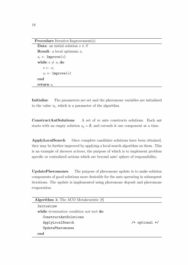
4.2.1 Pseudocode

Before presenting the metaheuristic formally, I will present it in pseudocode (see

Algorithm 1) and explain what the different components do.

18

Procedure Iterative-Improvement(s)

Data: an initial solution s ∈ SResult: a local optimum si

si ← Improve(s)

while s 6= si do

s ← si

si ← Improve(s)

end

return si

Initialize The parameters are set and the pheromone variables are initialized

to the value τ0, which is a parameter of the algorithm.

ConstructAntSolutions A set of m ants constructs solutions. Each ant

starts with an empty solution sp = ∅, and extends it one component at a time.

ApplyLocalSearch Once complete candidate solutions have been obtained,

they may be further improved by applying a local search algorithm on them. This

is an example of daemon actions, the purpose of which is to implement problem

specific or centralized actions which are beyond ants’ sphere of responsibility.

UpdatePheromones The purpose of pheromone update is to make solution

components of good solutions more desirable for the ants operating in subsequent

iterations. The update is implemented using pheromone deposit and pheromone

evaporation.

Algorithm 1: The ACO Metaheuristic [8]

Initialize

while termination condition not met do

ConstructAntSolutions

ApplyLocalSearch /* optional */

UpdatePheromones

end

19

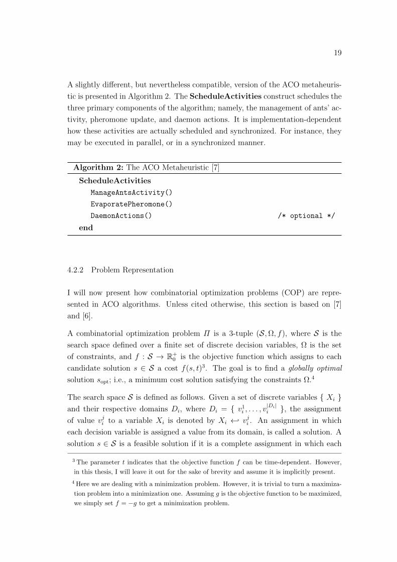
A slightly different, but nevertheless compatible, version of the ACO metaheuris-

tic is presented in Algorithm 2. The ScheduleActivities construct schedules the

three primary components of the algorithm; namely, the management of ants’ ac-

tivity, pheromone update, and daemon actions. It is implementation-dependent

how these activities are actually scheduled and synchronized. For instance, they

may be executed in parallel, or in a synchronized manner.

Algorithm 2: The ACO Metaheuristic [7]

ScheduleActivities

ManageAntsActivity()

EvaporatePheromone()

DaemonActions() /* optional */

end

4.2.2 Problem Representation

I will now present how combinatorial optimization problems (COP) are repre-

sented in ACO algorithms. Unless cited otherwise, this section is based on [7]

and [6].

A combinatorial optimization problem Π is a 3-tuple (S,Ω, f), where S is the

search space defined over a finite set of discrete decision variables, Ω is the set

of constraints, and f : S → R+0 is the objective function which assigns to each

candidate solution s ∈ S a cost f(s, t)3. The goal is to find a globally optimal

solution sopt; i.e., a minimum cost solution satisfying the constraints Ω.4

The search space S is defined as follows. Given a set of discrete variables Xi and their respective domains Di, where Di = v1i , . . . , v

|Di|i , the assignment

of value vji to a variable Xi is denoted by Xi ← vji . An assignment in which

each decision variable is assigned a value from its domain, is called a solution. A

solution s ∈ S is a feasible solution if it is a complete assignment in which each

3 The parameter t indicates that the objective function f can be time-dependent. However,

in this thesis, I will leave it out for the sake of brevity and assume it is implicitly present.

4 Here we are dealing with a minimization problem. However, it is trivial to turn a maximiza-

tion problem into a minimization one. Assuming g is the objective function to be maximized,

we simply set f = −g to get a minimization problem.

20

decision variable is assigned a value which satisfies all the constraints in Ω. If

the set Ω is empty, Π is said to be unconstrained. If the constraints cannot be

violated, they are called hard constraints; if they may be violated (possibly with

a penalty), they are called soft constraints.

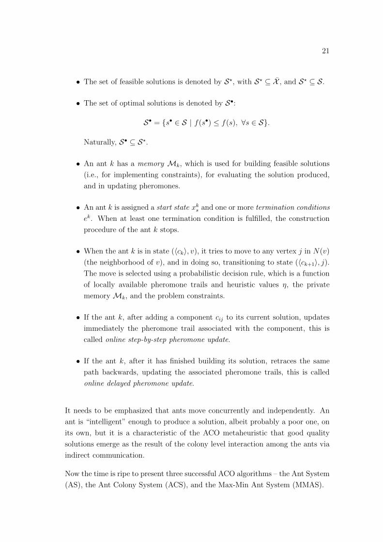
Some observations and definitions will follow.

• An instantiated decision variable Xi ← vji is called a solution component,

and is denoted by cij. The set of all possible solution components is denoted

by C.

• Ants traverse what is called the construction graph G = (V,E). The set

of components C may be associated either with the vertices V , or with the

edges E. The graph G is complete and connected.

• The states of the problem are defined in terms of sequences 〈c1, c2, . . . , ck〉(abbreviated as 〈ck〉, for some positive integer k) of elements of C, and in

terms of vertices of G. For instance, (〈ck〉, v) denotes the state where v

is the vertex the ant is at, and the sequence 〈ck〉 represents the (partial)

solution the ant has built so far. The set of all possible sequences is denoted

by X .

• A pheromone trail parameter Tij is associated with each component cij.

The value of Tij is denoted by τij and is called pheromone value.5 The

pheromone values are used and updated during the execution of an ACO

algorithm.

• A heuristic value ηij may be associated with each component cij. Heuris-

tic values represent a priori knowledge of the problem instance or of the

problem domain.

• The set of candidate solutions S is a subset of X .

• The finite set of constraints Ω defines the set of feasible states X , with

X ⊆ X .

5 Note that a pheromone value is generally a function of the algorithm’s iteration t:

τij = τij(t).

I assume the parameter t to be implicit for the sake of simplicity.

21

• The set of feasible solutions is denoted by S?, with S? ⊆ X , and S? ⊆ S.

• The set of optimal solutions is denoted by S•:

S• = s• ∈ S | f(s•) ≤ f(s), ∀s ∈ S.

Naturally, S• ⊆ S?.

• An ant k has a memory Mk, which is used for building feasible solutions

(i.e., for implementing constraints), for evaluating the solution produced,

and in updating pheromones.

• An ant k is assigned a start state xks and one or more termination conditions

ek. When at least one termination condition is fulfilled, the construction

procedure of the ant k stops.

• When the ant k is in state (〈ck〉, v), it tries to move to any vertex j in N(v)

(the neighborhood of v), and in doing so, transitioning to state (〈ck+1〉, j).The move is selected using a probabilistic decision rule, which is a function

of locally available pheromone trails and heuristic values η, the private

memory Mk, and the problem constraints.

• If the ant k, after adding a component cij to its current solution, updates

immediately the pheromone trail associated with the component, this is

called online step-by-step pheromone update.

• If the ant k, after it has finished building its solution, retraces the same

path backwards, updating the associated pheromone trails, this is called

online delayed pheromone update.

It needs to be emphasized that ants move concurrently and independently. An

ant is “intelligent” enough to produce a solution, albeit probably a poor one, on

its own, but it is a characteristic of the ACO metaheuristic that good quality

solutions emerge as the result of the colony level interaction among the ants via

indirect communication.

Now the time is ripe to present three successful ACO algorithms – the Ant System

(AS), the Ant Colony System (ACS), and the Max-Min Ant System (MMAS).

22

4.3 Ant System

The Ant System, the first ACO algorithm proposed in the literature [6], is the

progenitor of all the research efforts with ant algorithms [5]. As a matter of

fact, the AS was originally a set of three algorithms called the ant-cycle, the ant-

density, and the ant-quantity [7], but as the ant-cycle turned out to be superior

to the other two, performance-wise, it attracted more attention [3]. Thus ant-

cycle would later be called simply the Ant System, whereas ant-density and

ant-quantity have gradually fallen into oblivion [8].

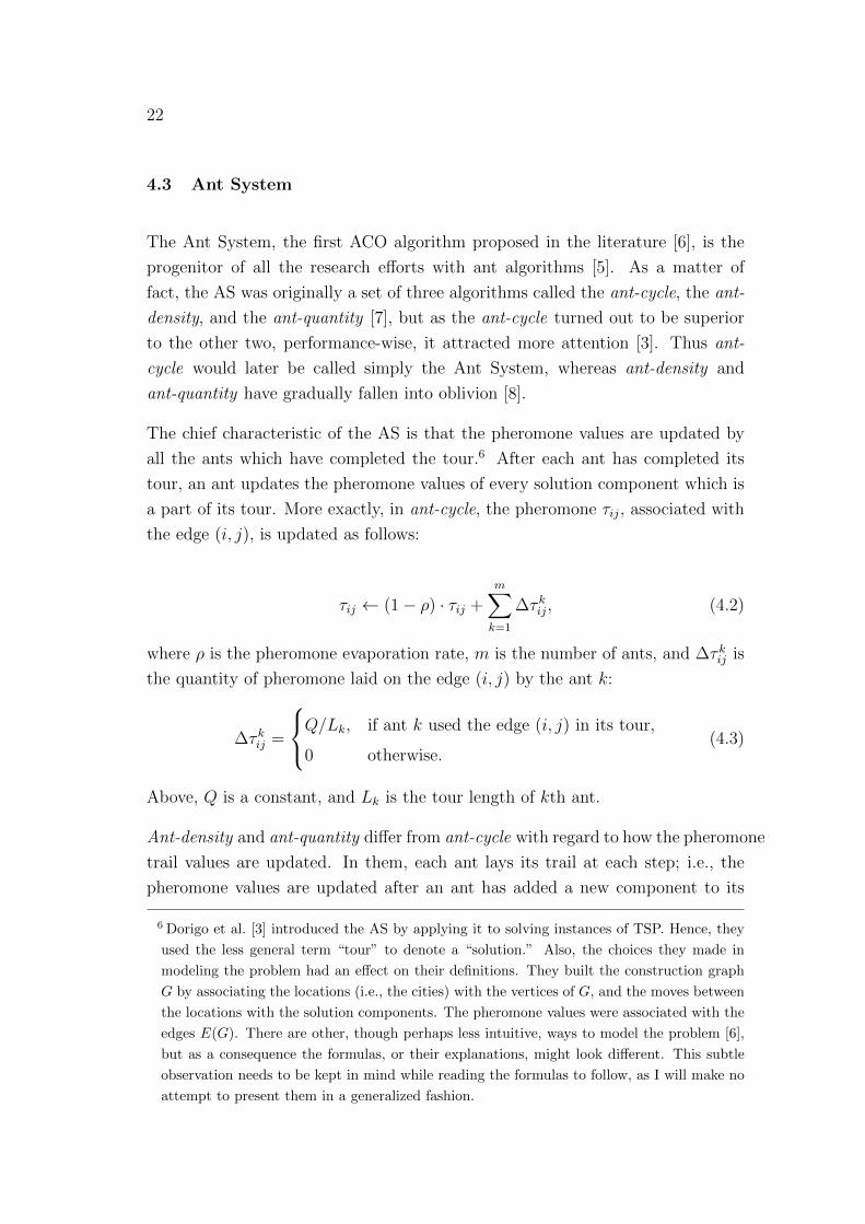
The chief characteristic of the AS is that the pheromone values are updated by

all the ants which have completed the tour.6 After each ant has completed its

tour, an ant updates the pheromone values of every solution component which is

a part of its tour. More exactly, in ant-cycle, the pheromone τij, associated with

the edge (i, j), is updated as follows:

τij ← (1− ρ) · τij +m∑k=1

∆τ kij, (4.2)

where ρ is the pheromone evaporation rate, m is the number of ants, and ∆τ kij is

the quantity of pheromone laid on the edge (i, j) by the ant k:

∆τ kij =

Q/Lk, if ant k used the edge (i, j) in its tour,

0 otherwise.(4.3)

Above, Q is a constant, and Lk is the tour length of kth ant.

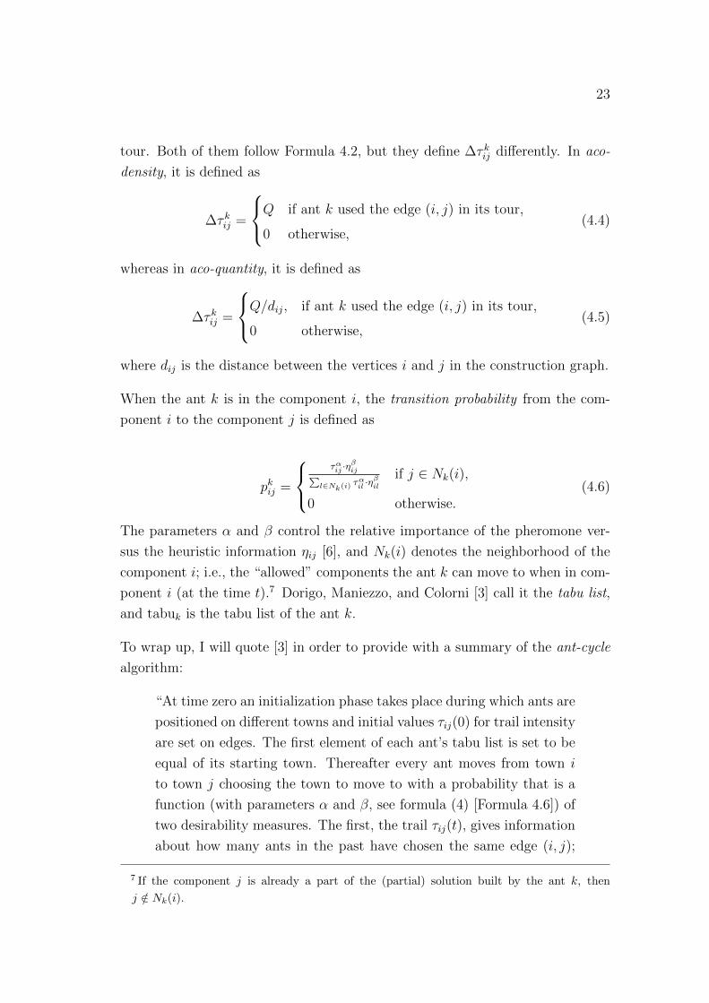
Ant-density and ant-quantity differ from ant-cycle with regard to how the pheromone

trail values are updated. In them, each ant lays its trail at each step; i.e., the

pheromone values are updated after an ant has added a new component to its

6 Dorigo et al. [3] introduced the AS by applying it to solving instances of TSP. Hence, they

used the less general term “tour” to denote a “solution.” Also, the choices they made in

modeling the problem had an effect on their definitions. They built the construction graph

G by associating the locations (i.e., the cities) with the vertices of G, and the moves between

the locations with the solution components. The pheromone values were associated with the

edges E(G). There are other, though perhaps less intuitive, ways to model the problem [6],

but as a consequence the formulas, or their explanations, might look different. This subtle

observation needs to be kept in mind while reading the formulas to follow, as I will make no

attempt to present them in a generalized fashion.

23

tour. Both of them follow Formula 4.2, but they define ∆τ kij differently. In aco-

density, it is defined as

∆τ kij =

Q if ant k used the edge (i, j) in its tour,

0 otherwise,(4.4)

whereas in aco-quantity, it is defined as

∆τ kij =

Q/dij, if ant k used the edge (i, j) in its tour,

0 otherwise,(4.5)

where dij is the distance between the vertices i and j in the construction graph.

When the ant k is in the component i, the transition probability from the com-

ponent i to the component j is defined as

pkij =

ταij ·η

βij∑

l∈Nk(i)ταil ·η

βil

if j ∈ Nk(i),

0 otherwise.(4.6)

The parameters α and β control the relative importance of the pheromone ver-

sus the heuristic information ηij [6], and Nk(i) denotes the neighborhood of the

component i; i.e., the “allowed” components the ant k can move to when in com-

ponent i (at the time t).7 Dorigo, Maniezzo, and Colorni [3] call it the tabu list,

and tabuk is the tabu list of the ant k.

To wrap up, I will quote [3] in order to provide with a summary of the ant-cycle

algorithm:

“At time zero an initialization phase takes place during which ants are

positioned on different towns and initial values τij(0) for trail intensity

are set on edges. The first element of each ant’s tabu list is set to be

equal of its starting town. Thereafter every ant moves from town i

to town j choosing the town to move to with a probability that is a

function (with parameters α and β, see formula (4) [Formula 4.6]) of

two desirability measures. The first, the trail τij(t), gives information

about how many ants in the past have chosen the same edge (i, j);

7 If the component j is already a part of the (partial) solution built by the ant k, then

j /∈ Nk(i).

24

the second, the visibility ηij, says that the closer a town the more

desirable it is. [- -]

“After n iterations all ants have completed a tour, and their tabu lists

will be full; at this point for each ant k the value of Lk is computed and

the values ∆τ kij are updated according to formula (3) [Formula 4.3].

Also, the shortest path found by the ants [- -] is saved and all the

tabu lists are emptied. This process is iterated until the tour counter

reaches the maximum (user-defined) number of cycles NCMAX, or all

the ants make the same tour.”

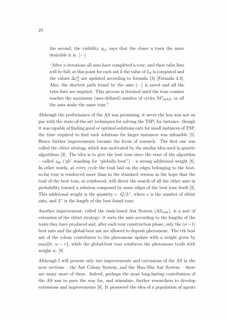
Although the performance of the AS was promising, it never the less was not on

par with the state-of-the-art techniques for solving the TSP; for instance, though

it was capable of finding good or optimal solutions only for small instances of TSP,

the time required to find such solutions for larger instances was infeasible [5].

Hence further improvements became the focus of research. The first one was

called the elitist strategy, which was motivated by the similar idea used in genetic

algorithms [3]. The idea is to give the best tour since the start of the algorithm

– called sgb (‘gb’ standing for “globally-best”) – a strong additional weight [8].

In other words, at every cycle the trail laid on the edges belonging to the best-

so-far tour is reinforced more than in the standard version in the hope that the

trail of the best tour, so reinforced, will direct the search of all the other ants in

probability toward a solution composed by some edges of the best tour itself [3].

This additional weight is the quantity e · Q/L∗, where e is the number of elitist

ants, and L∗ is the length of the best found tour.

Another improvement, called the rank-based Ant System (ASrank), is a sort of

extension of the elitist strategy: it sorts the ants according to the lengths of the

tours they have produced and, after each tour construction phase, only the (w−1)

best ants and the global-best ant are allowed to deposit pheromone. The rth best

ant of the colony contributes to the pheromone update with a weight given by

max0, w − r, while the global-best tour reinforces the pheromone trails with

weight w. [8]

Although I will present only two improvements and extensions of the AS in the

next sections – the Ant Colony System, and the Max-Min Ant System – there

are many more of them. Indeed, perhaps the most long-lasting contribution of

the AS was to pave the way for, and stimulate, further researchers to develop

extensions and improvements [8]. It pioneered the idea of a population of agents

25

each guided by an autocatalytic process directed by a greedy force [3], and of the

synergistic use of cooperation among these simple agents which communicate via

a non-symbolic medium [5].

4.4 Ant Colony System

The ACS algorithm was expressly devised to improve the efficiency of the AS to

solve instances of symmetric and asymmetric TSP [5]. It differs from preceding

ant algorithms in three respects: (i) the state transition rule provides a direct

way to balance between exploration of new edges and exploitation of a priori and

accumulated knowledge of the problem; (ii) the global updating rule is applied only

to edges belonging to the best ant tour; and (iii) while ants construct a solution

a local pheromone updating rule is applied. [5]

In the following quotation, the developers of the ACS algorithm themselves ex-

plain in “layman terms” how the algorithm works [5]:

“m ants are initially positioned on n cities chosen according to some

initialization rule (e.g., randomly). Each ant builds a tour (i.e., a fea-

sible solution to the TSP) by repeatedly applying a stochastic greedy

rule (the state transition rule). While constructing its tour, an ant

also modifies the amount of pheromone on the visited edges by apply-

ing the local updating rule. Once all ants have terminated their tour,

the amount of pheromone on edges is modified again (by applying the

global updating rule). As was the case in ant system, ants are guided,

in building their tours, by both heuristic information (they prefer to

choose short edges), and by pheromone information: An edge with a

high amount of pheromone is a very desirable choice. The pheromone

updating rules are designed so that they tend to give more pheromone

to edges which should be visited by ants.”

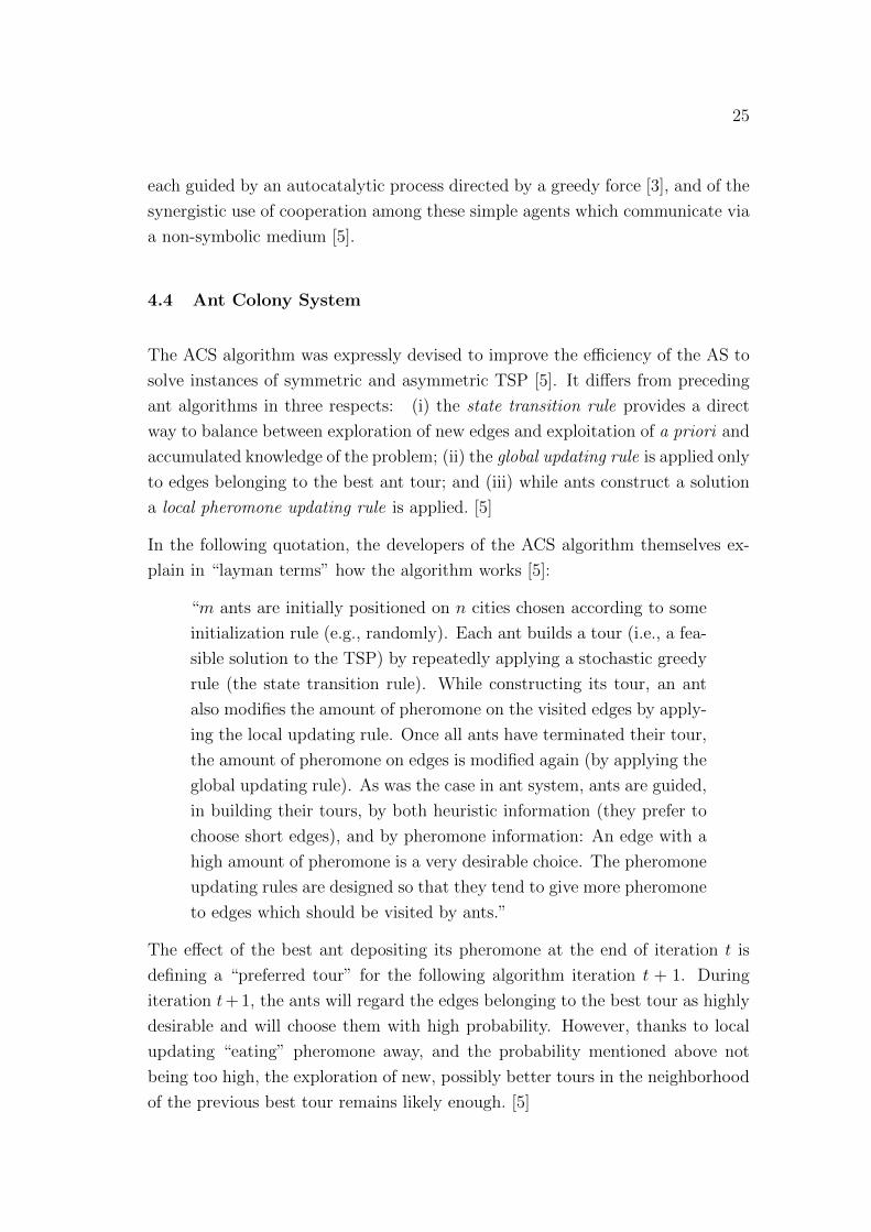
The effect of the best ant depositing its pheromone at the end of iteration t is

defining a “preferred tour” for the following algorithm iteration t + 1. During

iteration t+ 1, the ants will regard the edges belonging to the best tour as highly

desirable and will choose them with high probability. However, thanks to local

updating “eating” pheromone away, and the probability mentioned above not

being too high, the exploration of new, possibly better tours in the neighborhood

of the previous best tour remains likely enough. [5]

26

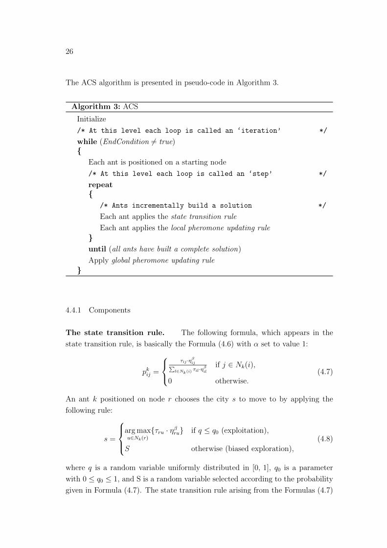
The ACS algorithm is presented in pseudo-code in Algorithm 3.

Algorithm 3: ACS

Initialize

/* At this level each loop is called an ‘iteration’ */

while (EndCondition 6= true)

Each ant is positioned on a starting node

/* At this level each loop is called an ‘step’ */

repeat

/* Ants incrementally build a solution */

Each ant applies the state transition rule

Each ant applies the local pheromone updating rule

until (all ants have built a complete solution)

Apply global pheromone updating rule

4.4.1 Components

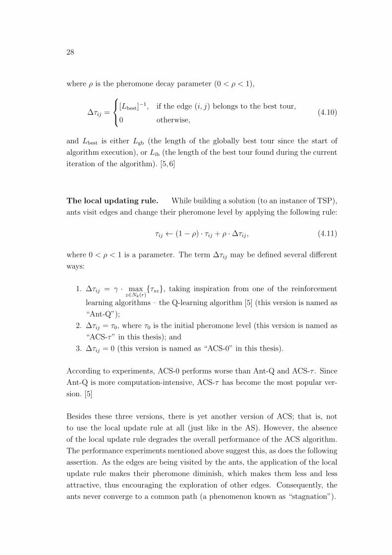
The state transition rule. The following formula, which appears in the

state transition rule, is basically the Formula (4.6) with α set to value 1:

pkij =

τij ·ηβij∑

l∈Nk(i)τil·ηβil

if j ∈ Nk(i),

0 otherwise.(4.7)

An ant k positioned on node r chooses the city s to move to by applying the

following rule:

s =

arg maxu∈Nk(r)

τru · ηβru if q ≤ q0 (exploitation),

S otherwise (biased exploration),

(4.8)

where q is a random variable uniformly distributed in [0, 1], q0 is a parameter

with 0 ≤ q0 ≤ 1, and S is a random variable selected according to the probability

given in Formula (4.7). The state transition rule arising from the Formulas (4.7)

27

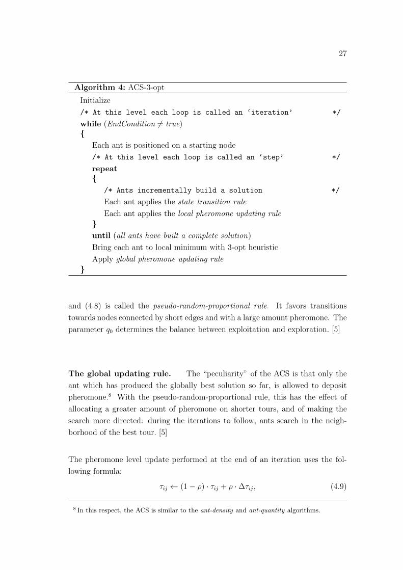
Algorithm 4: ACS-3-opt

Initialize

/* At this level each loop is called an ‘iteration’ */

while (EndCondition 6= true)

Each ant is positioned on a starting node

/* At this level each loop is called an ‘step’ */

repeat

/* Ants incrementally build a solution */

Each ant applies the state transition rule

Each ant applies the local pheromone updating rule

until (all ants have built a complete solution)

Bring each ant to local minimum with 3-opt heuristic

Apply global pheromone updating rule

and (4.8) is called the pseudo-random-proportional rule. It favors transitions

towards nodes connected by short edges and with a large amount pheromone. The

parameter q0 determines the balance between exploitation and exploration. [5]

The global updating rule. The “peculiarity” of the ACS is that only the

ant which has produced the globally best solution so far, is allowed to deposit

pheromone.8 With the pseudo-random-proportional rule, this has the effect of

allocating a greater amount of pheromone on shorter tours, and of making the

search more directed: during the iterations to follow, ants search in the neigh-

borhood of the best tour. [5]

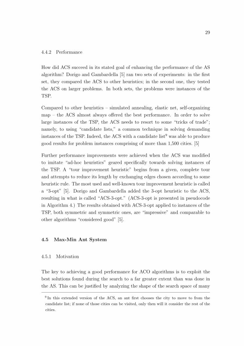
The pheromone level update performed at the end of an iteration uses the fol-

lowing formula:

τij ← (1− ρ) · τij + ρ ·∆τij, (4.9)

8 In this respect, the ACS is similar to the ant-density and ant-quantity algorithms.

28

where ρ is the pheromone decay parameter (0 < ρ < 1),

∆τij =

[Lbest]−1, if the edge (i, j) belongs to the best tour,

0 otherwise,(4.10)

and Lbest is either Lgb (the length of the globally best tour since the start of

algorithm execution), or Lib (the length of the best tour found during the current

iteration of the algorithm). [5, 6]

The local updating rule. While building a solution (to an instance of TSP),

ants visit edges and change their pheromone level by applying the following rule:

τij ← (1− ρ) · τij + ρ ·∆τij, (4.11)

where 0 < ρ < 1 is a parameter. The term ∆τij may be defined several different

ways:

1. ∆τij = γ · maxz∈Nk(r)

τsz, taking inspiration from one of the reinforcement

learning algorithms – the Q-learning algorithm [5] (this version is named as

“Ant-Q”);

2. ∆τij = τ0, where τ0 is the initial pheromone level (this version is named as

“ACS-τ” in this thesis); and

3. ∆τij = 0 (this version is named as “ACS-0” in this thesis).

According to experiments, ACS-0 performs worse than Ant-Q and ACS-τ . Since

Ant-Q is more computation-intensive, ACS-τ has become the most popular ver-

sion. [5]

Besides these three versions, there is yet another version of ACS; that is, not

to use the local update rule at all (just like in the AS). However, the absence

of the local update rule degrades the overall performance of the ACS algorithm.

The performance experiments mentioned above suggest this, as does the following

assertion. As the edges are being visited by the ants, the application of the local

update rule makes their pheromone diminish, which makes them less and less

attractive, thus encouraging the exploration of other edges. Consequently, the

ants never converge to a common path (a phenomenon known as “stagnation”).

29

4.4.2 Performance

How did ACS succeed in its stated goal of enhancing the performance of the AS

algorithm? Dorigo and Gambardella [5] ran two sets of experiments: in the first

set, they compared the ACS to other heuristics; in the second one, they tested

the ACS on larger problems. In both sets, the problems were instances of the

TSP.

Compared to other heuristics – simulated annealing, elastic net, self-organizing

map – the ACS almost always offered the best performance. In order to solve

large instances of the TSP, the ACS needs to resort to some “tricks of trade”;

namely, to using “candidate lists,” a common technique in solving demanding

instances of the TSP. Indeed, the ACS with a candidate list9 was able to produce

good results for problem instances comprising of more than 1,500 cities. [5]

Further performance improvements were achieved when the ACS was modified

to imitate “ad-hoc heuristics” geared specifically towards solving instances of

the TSP. A “tour improvement heuristic” begins from a given, complete tour

and attempts to reduce its length by exchanging edges chosen according to some

heuristic rule. The most used and well-known tour improvement heuristic is called

a “3-opt” [5]. Dorigo and Gambardella added the 3-opt heuristic to the ACS,

resulting in what is called “ACS-3-opt.” (ACS-3-opt is presented in pseudocode

in Algorithm 4.) The results obtained with ACS-3-opt applied to instances of the

TSP, both symmetric and symmetric ones, are “impressive” and comparable to

other algorithms “considered good” [5].

4.5 Max-Min Ant System

4.5.1 Motivation

The key to achieving a good performance for ACO algorithms is to exploit the

best solutions found during the search to a far greater extent than was done in

the AS. This can be justified by analyzing the shape of the search space of many

9 In this extended version of the ACS, an ant first chooses the city to move to from the

candidate list; if none of those cities can be visited, only then will it consider the rest of the

cities.

30

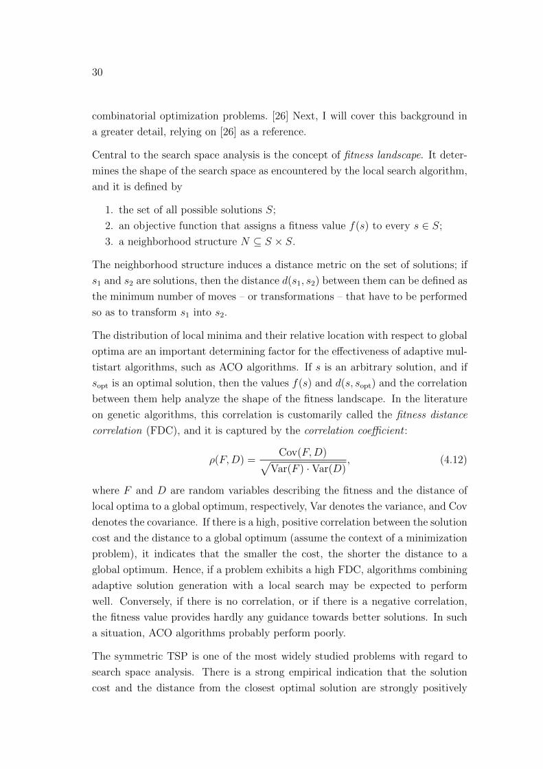
combinatorial optimization problems. [26] Next, I will cover this background in

a greater detail, relying on [26] as a reference.

Central to the search space analysis is the concept of fitness landscape. It deter-

mines the shape of the search space as encountered by the local search algorithm,

and it is defined by

1. the set of all possible solutions S;

2. an objective function that assigns a fitness value f(s) to every s ∈ S;

3. a neighborhood structure N ⊆ S × S.

The neighborhood structure induces a distance metric on the set of solutions; if

s1 and s2 are solutions, then the distance d(s1, s2) between them can be defined as

the minimum number of moves – or transformations – that have to be performed

so as to transform s1 into s2.

The distribution of local minima and their relative location with respect to global

optima are an important determining factor for the effectiveness of adaptive mul-

tistart algorithms, such as ACO algorithms. If s is an arbitrary solution, and if

sopt is an optimal solution, then the values f(s) and d(s, sopt) and the correlation

between them help analyze the shape of the fitness landscape. In the literature

on genetic algorithms, this correlation is customarily called the fitness distance

correlation (FDC), and it is captured by the correlation coefficient :

ρ(F,D) =Cov(F,D)√

Var(F ) · Var(D), (4.12)

where F and D are random variables describing the fitness and the distance of

local optima to a global optimum, respectively, Var denotes the variance, and Cov

denotes the covariance. If there is a high, positive correlation between the solution

cost and the distance to a global optimum (assume the context of a minimization

problem), it indicates that the smaller the cost, the shorter the distance to a

global optimum. Hence, if a problem exhibits a high FDC, algorithms combining

adaptive solution generation with a local search may be expected to perform

well. Conversely, if there is no correlation, or if there is a negative correlation,

the fitness value provides hardly any guidance towards better solutions. In such

a situation, ACO algorithms probably perform poorly.

The symmetric TSP is one of the most widely studied problems with regard to

search space analysis. There is a strong empirical indication that the solution

cost and the distance from the closest optimal solution are strongly positively

31

correlated in the TSP.10 This, in turn, indicates that locally optimal tours are

concentrated around a small region of the entire search space. Therefore, it makes

sense to “focus” ants’ attention and efforts to the best tours (either iteration-best

or globally-best). It is this observation which is behind many of the design choices

of MMAS.

4.5.2 Algorithm

Stutzle and Hoos [26] describe the requirements the MMAS was designed to meet

as follows:

“Research on ACO has shown that improved performance may be ob-

tained by a stronger exploitation of the best solutions found during

the search and the search space analysis [- -] gives an explanation

of this fact. Yet, using a greedier search potentially aggravates the

problem of premature stagnation of the search. Therefore, the key

to achieve best performance of ACO algorithms is to combine an im-

proved exploitation of the best solutions found during the search with

an effective mechanism for avoiding early search stagnation.”

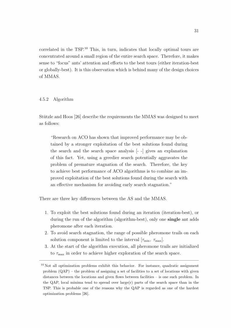
There are three key differences between the AS and the MMAS.

1. To exploit the best solutions found during an iteration (iteration-best), or

during the run of the algorithm (algorithm-best), only one single ant adds

pheromone after each iteration.

2. To avoid search stagnation, the range of possible pheromone trails on each

solution component is limited to the interval [τmin, τmax].

3. At the start of the algorithm execution, all pheromone trails are initialized

to τmax in order to achieve higher exploration of the search space.

10 Not all optimization problems exhibit this behavior. For instance, quadratic assignment

problem (QAP) – the problem of assigning a set of facilities to a set of locations with given

distances between the locations and given flows between facilities – is one such problem. In

the QAP, local minima tend to spread over large(r) parts of the search space than in the

TSP. This is probable one of the reasons why the QAP is regarded as one of the hardest

optimization problems [26].

32

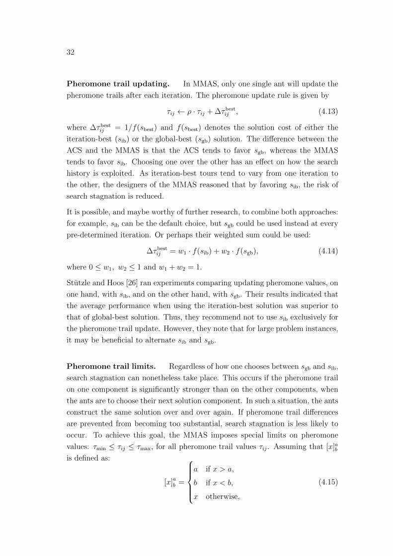
Pheromone trail updating. In MMAS, only one single ant will update the

pheromone trails after each iteration. The pheromone update rule is given by

τij ← ρ · τij + ∆τbestij , (4.13)

where ∆τbestij = 1/f(sbest) and f(sbest) denotes the solution cost of either the

iteration-best (sib) or the global-best (sgb) solution. The difference between the

ACS and the MMAS is that the ACS tends to favor sgb, whereas the MMAS

tends to favor sib. Choosing one over the other has an effect on how the search

history is exploited. As iteration-best tours tend to vary from one iteration to

the other, the designers of the MMAS reasoned that by favoring sib, the risk of

search stagnation is reduced.

It is possible, and maybe worthy of further research, to combine both approaches:

for example, sib can be the default choice, but sgb could be used instead at every

pre-determined iteration. Or perhaps their weighted sum could be used:

∆τbestij = w1 · f(sib) + w2 · f(sgb), (4.14)

where 0 ≤ w1, w2 ≤ 1 and w1 + w2 = 1.

Stutzle and Hoos [26] ran experiments comparing updating pheromone values, on

one hand, with sib, and on the other hand, with sgb. Their results indicated that

the average performance when using the iteration-best solution was superior to

that of global-best solution. Thus, they recommend not to use sib exclusively for

the pheromone trail update. However, they note that for large problem instances,

it may be beneficial to alternate sib and sgb.

Pheromone trail limits. Regardless of how one chooses between sgb and sib,

search stagnation can nonetheless take place. This occurs if the pheromone trail

on one component is significantly stronger than on the other components, when

the ants are to choose their next solution component. In such a situation, the ants

construct the same solution over and over again. If pheromone trail differences

are prevented from becoming too substantial, search stagnation is less likely to

occur. To achieve this goal, the MMAS imposes special limits on pheromone

values: τmin ≤ τij ≤ τmax, for all pheromone trail values τij. Assuming that [x]abis defined as:

[x]ab =

a if x > a,

b if x < b,

x otherwise,

(4.15)

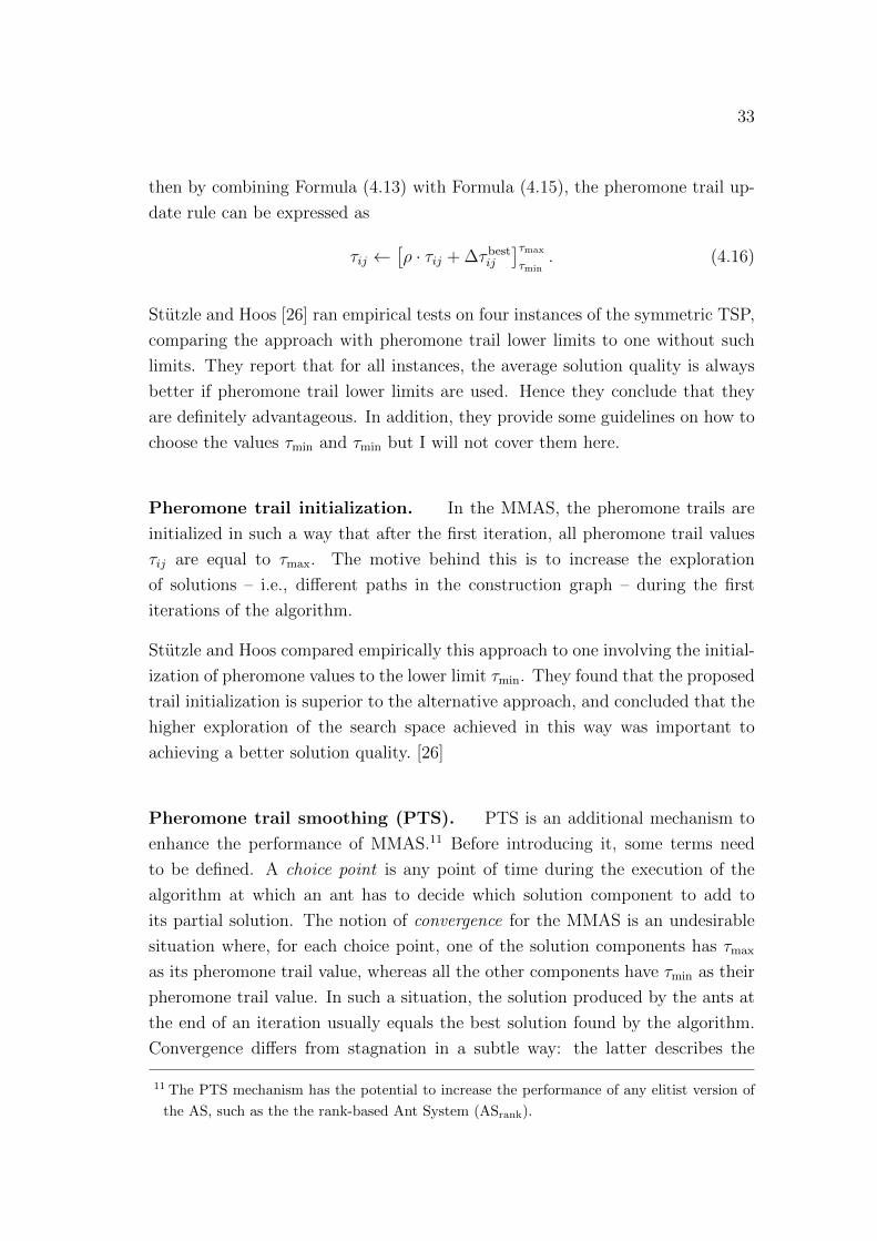
33

then by combining Formula (4.13) with Formula (4.15), the pheromone trail up-

date rule can be expressed as

τij ←[ρ · τij + ∆τbestij

]τmax

τmin. (4.16)

Stutzle and Hoos [26] ran empirical tests on four instances of the symmetric TSP,

comparing the approach with pheromone trail lower limits to one without such

limits. They report that for all instances, the average solution quality is always

better if pheromone trail lower limits are used. Hence they conclude that they

are definitely advantageous. In addition, they provide some guidelines on how to

choose the values τmin and τmin but I will not cover them here.

Pheromone trail initialization. In the MMAS, the pheromone trails are

initialized in such a way that after the first iteration, all pheromone trail values

τij are equal to τmax. The motive behind this is to increase the exploration

of solutions – i.e., different paths in the construction graph – during the first

iterations of the algorithm.

Stutzle and Hoos compared empirically this approach to one involving the initial-

ization of pheromone values to the lower limit τmin. They found that the proposed

trail initialization is superior to the alternative approach, and concluded that the

higher exploration of the search space achieved in this way was important to

achieving a better solution quality. [26]

Pheromone trail smoothing (PTS). PTS is an additional mechanism to

enhance the performance of MMAS.11 Before introducing it, some terms need

to be defined. A choice point is any point of time during the execution of the

algorithm at which an ant has to decide which solution component to add to

its partial solution. The notion of convergence for the MMAS is an undesirable

situation where, for each choice point, one of the solution components has τmax

as its pheromone trail value, whereas all the other components have τmin as their

pheromone trail value. In such a situation, the solution produced by the ants at

the end of an iteration usually equals the best solution found by the algorithm.

Convergence differs from stagnation in a subtle way: the latter describes the

11 The PTS mechanism has the potential to increase the performance of any elitist version of

the AS, such as the the rank-based Ant System (ASrank).

34

situation where all the ants follow the same path; this does not happen in the

convergence of the MMAS thanks to the use of pheromone trail limits.

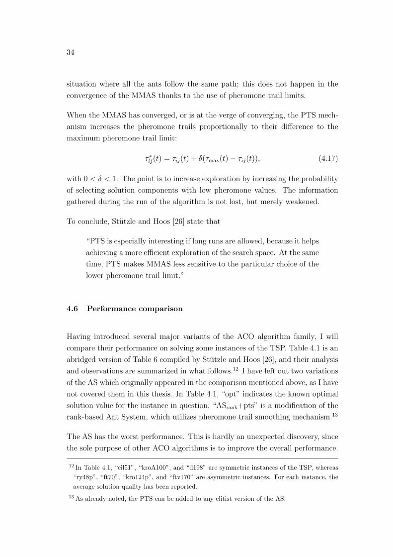
When the MMAS has converged, or is at the verge of converging, the PTS mech-

anism increases the pheromone trails proportionally to their difference to the

maximum pheromone trail limit:

τ ∗ij(t) = τij(t) + δ(τmax(t)− τij(t)), (4.17)

with 0 < δ < 1. The point is to increase exploration by increasing the probability

of selecting solution components with low pheromone values. The information

gathered during the run of the algorithm is not lost, but merely weakened.

To conclude, Stutzle and Hoos [26] state that

“PTS is especially interesting if long runs are allowed, because it helps

achieving a more efficient exploration of the search space. At the same

time, PTS makes MMAS less sensitive to the particular choice of the

lower pheromone trail limit.”

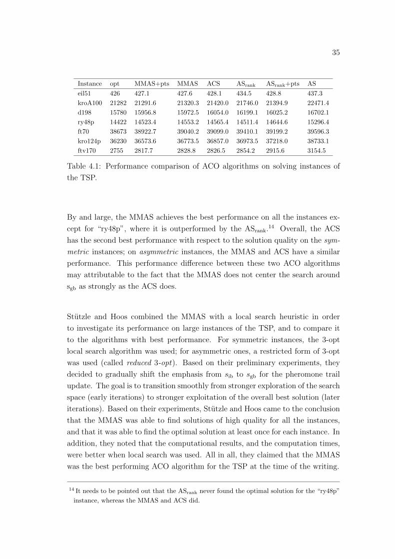
4.6 Performance comparison

Having introduced several major variants of the ACO algorithm family, I will

compare their performance on solving some instances of the TSP. Table 4.1 is an

abridged version of Table 6 compiled by Stutzle and Hoos [26], and their analysis

and observations are summarized in what follows.12 I have left out two variations

of the AS which originally appeared in the comparison mentioned above, as I have

not covered them in this thesis. In Table 4.1, “opt” indicates the known optimal

solution value for the instance in question; “ASrank+pts” is a modification of the

rank-based Ant System, which utilizes pheromone trail smoothing mechanism.13

The AS has the worst performance. This is hardly an unexpected discovery, since

the sole purpose of other ACO algorithms is to improve the overall performance.

12 In Table 4.1, “eil51”, “kroA100”, and “d198” are symmetric instances of the TSP, whereas

“ry48p”, “ft70”, “kro124p”, and “ftv170” are asymmetric instances. For each instance, the

average solution quality has been reported.

13 As already noted, the PTS can be added to any elitist version of the AS.

35

Instance opt MMAS+pts MMAS ACS ASrank ASrank+pts AS

eil51 426 427.1 427.6 428.1 434.5 428.8 437.3

kroA100 21282 21291.6 21320.3 21420.0 21746.0 21394.9 22471.4

d198 15780 15956.8 15972.5 16054.0 16199.1 16025.2 16702.1

ry48p 14422 14523.4 14553.2 14565.4 14511.4 14644.6 15296.4

ft70 38673 38922.7 39040.2 39099.0 39410.1 39199.2 39596.3

kro124p 36230 36573.6 36773.5 36857.0 36973.5 37218.0 38733.1

ftv170 2755 2817.7 2828.8 2826.5 2854.2 2915.6 3154.5

Table 4.1: Performance comparison of ACO algorithms on solving instances of

the TSP.

By and large, the MMAS achieves the best performance on all the instances ex-

cept for “ry48p”, where it is outperformed by the ASrank.14 Overall, the ACS

has the second best performance with respect to the solution quality on the sym-

metric instances; on asymmetric instances, the MMAS and ACS have a similar

performance. This performance difference between these two ACO algorithms

may attributable to the fact that the MMAS does not center the search around

sgb as strongly as the ACS does.

Stutzle and Hoos combined the MMAS with a local search heuristic in order

to investigate its performance on large instances of the TSP, and to compare it

to the algorithms with best performance. For symmetric instances, the 3-opt

local search algorithm was used; for asymmetric ones, a restricted form of 3-opt

was used (called reduced 3-opt). Based on their preliminary experiments, they

decided to gradually shift the emphasis from sib to sgb for the pheromone trail

update. The goal is to transition smoothly from stronger exploration of the search

space (early iterations) to stronger exploitation of the overall best solution (later

iterations). Based on their experiments, Stutzle and Hoos came to the conclusion

that the MMAS was able to find solutions of high quality for all the instances,

and that it was able to find the optimal solution at least once for each instance. In

addition, they noted that the computational results, and the computation times,

were better when local search was used. All in all, they claimed that the MMAS

was the best performing ACO algorithm for the TSP at the time of the writing.

14 It needs to be pointed out that the ASrank never found the optimal solution for the “ry48p”

instance, whereas the MMAS and ACS did.

36

4.7 Theoretical Results

Empirical results have shown that ACO algorithms are efficient at solving a vari-

ety of combinatorial optimization problems; however, there used to be very little

theory to explain why. Convergence proofs15 appeared several years after the

first variants of ACO algorithms had been presented. Gutjahr was among the

first people to prove the convergence to the globally optimal solution with prob-

ability 1 − ε. The downside of his proof was that is was applicable only to a

particular ACO algorithm – called the Graph-Based Ant System (GBAS) – and

hence it could not be generalized to other ACO algorithms. Moreover, there was

no empirical data available about the performance of GBAS. [25]

Fortunately, the limitations of the Gutjahr’s proof were overcome by Stutzle and

Dorigo [25], who discovered a convergence proof which applies directly to the

ACS and MMAS. To prove the convergence, they introduced an algorithm class

ACO-τmin, and a particular member of that class, called ACO-gb-τmin. They went

on to prove the convergence for ACO-gb-τmin, and then they generalized the proof

so that is applies to every member of ACO-τmin. (Naturally, they proved that

MMAS and ACS are members of ACO-τmin.)

In what follows, I will present the ACO-gb-τmin algorithm, define the ACO-τmin

algorithm class, and present the theorems and propositions of the convergence

proof.16 Unless otherwise cited, my presentation is based on the article by Stutzle

and Dorigo [25].

4.7.1 ACO-gb-τmin and ACO-τmin

The presentation to follow will make use of the terminology and notation intro-

duced in Subsection 4.2.2.

The procedure ‘ACO-Gb-Tau-Min’ (page 37) gives a high-level description of

ACO-gb-τmin. In the pseudocode, s will denote the best feasible solution found so

far, whereas st will denote the best feasible solution found during the tth iteration

of the algorithm.

15 A convergence proof means proving that during the execution of an ACO algorithm, the

ants will eventually produce the optimal solution, and nothing but the optimal solution.

16 I will omit the proofs of the theorems and propositions; instead, I will refer the reader to [25].

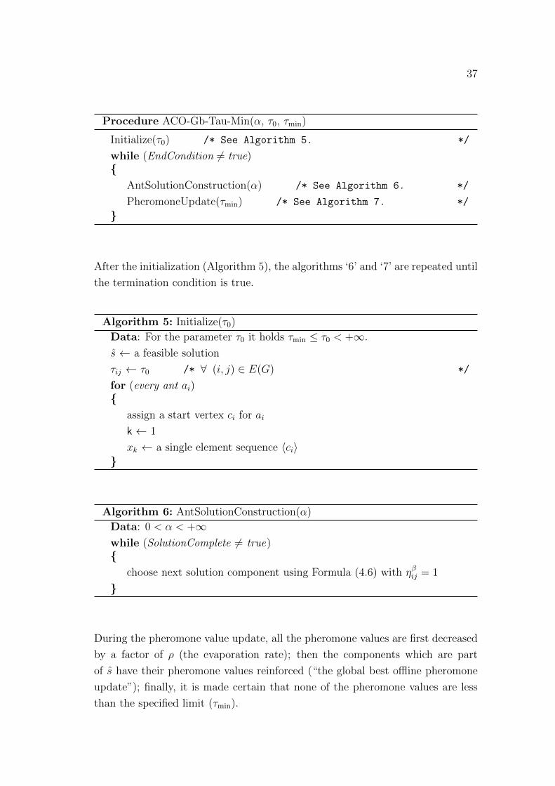
37

Procedure ACO-Gb-Tau-Min(α, τ0, τmin)

Initialize(τ0) /* See Algorithm 5. */

while (EndCondition 6= true)

AntSolutionConstruction(α) /* See Algorithm 6. */

PheromoneUpdate(τmin) /* See Algorithm 7. */

After the initialization (Algorithm 5), the algorithms ‘6’ and ‘7’ are repeated until

the termination condition is true.

Algorithm 5: Initialize(τ0)

Data: For the parameter τ0 it holds τmin ≤ τ0 < +∞.

s ← a feasible solution

τij ← τ0 /* ∀ (i, j) ∈ E(G) */

for (every ant ai)

assign a start vertex ci for ai

k ← 1

xk ← a single element sequence 〈ci〉

Algorithm 6: AntSolutionConstruction(α)

Data: 0 < α < +∞while (SolutionComplete 6= true)

choose next solution component using Formula (4.6) with ηβij = 1

During the pheromone value update, all the pheromone values are first decreased

by a factor of ρ (the evaporation rate); then the components which are part

of s have their pheromone values reinforced (“the global best offline pheromone

update”); finally, it is made certain that none of the pheromone values are less

than the specified limit (τmin).

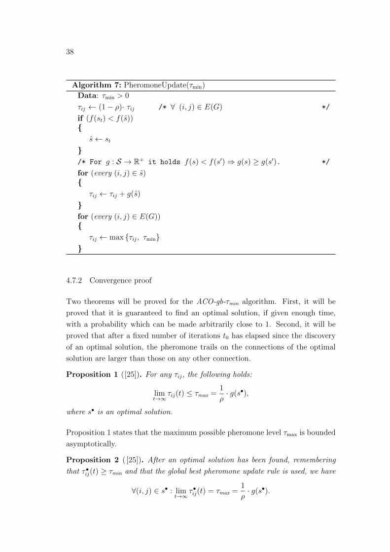
38

Algorithm 7: PheromoneUpdate(τmin)

Data: τmin > 0

τij ← (1− ρ)· τij /* ∀ (i, j) ∈ E(G) */

if (f(st) < f(s))

s← st

/* For g : S → R+ it holds f(s) < f(s′)⇒ g(s) ≥ g(s′). */

for (every (i, j) ∈ s)

τij ← τij + g(s)

for (every (i, j) ∈ E(G))

τij ← max τij, τmin

4.7.2 Convergence proof

Two theorems will be proved for the ACO-gb-τmin algorithm. First, it will be

proved that it is guaranteed to find an optimal solution, if given enough time,

with a probability which can be made arbitrarily close to 1. Second, it will be

proved that after a fixed number of iterations t0 has elapsed since the discovery

of an optimal solution, the pheromone trails on the connections of the optimal

solution are larger than those on any other connection.

Proposition 1 ([25]). For any τij, the following holds:

limt→∞

τij(t) ≤ τmax =1

ρ· g(s•),

where s• is an optimal solution.

Proposition 1 states that the maximum possible pheromone level τmax is bounded

asymptotically.

Proposition 2 ( [25]). After an optimal solution has been found, remembering

that τ •ij(t) ≥ τmin and that the global best pheromone update rule is used, we have

∀(i, j) ∈ s• : limt→∞

τ •ij(t) = τmax =1

ρ· g(s•).

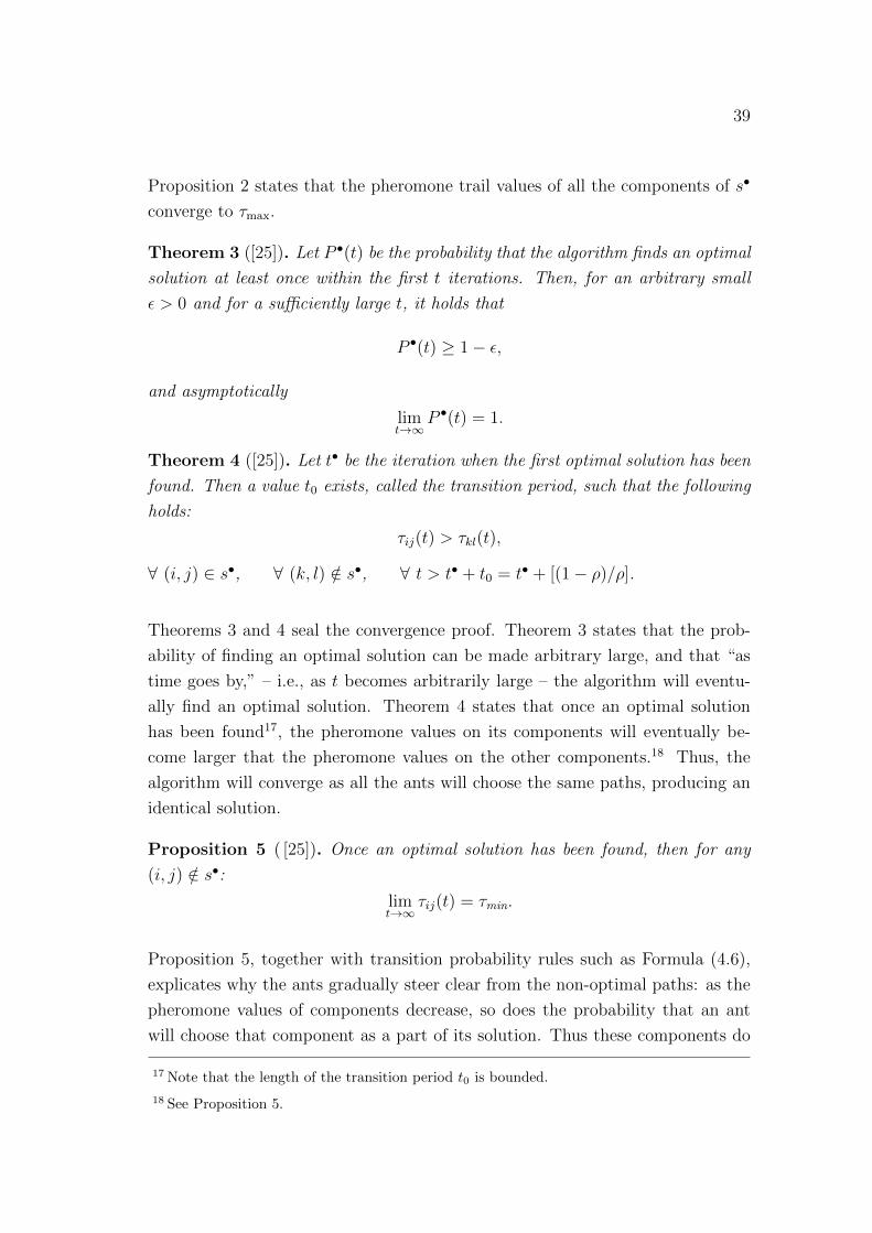
39

Proposition 2 states that the pheromone trail values of all the components of s•

converge to τmax.

Theorem 3 ([25]). Let P •(t) be the probability that the algorithm finds an optimal

solution at least once within the first t iterations. Then, for an arbitrary small

ε > 0 and for a sufficiently large t, it holds that

P •(t) ≥ 1− ε,

and asymptotically

limt→∞

P •(t) = 1.

Theorem 4 ([25]). Let t• be the iteration when the first optimal solution has been

found. Then a value t0 exists, called the transition period, such that the following

holds:

τij(t) > τkl(t),

∀ (i, j) ∈ s•, ∀ (k, l) /∈ s•, ∀ t > t• + t0 = t• + [(1− ρ)/ρ].

Theorems 3 and 4 seal the convergence proof. Theorem 3 states that the prob-

ability of finding an optimal solution can be made arbitrary large, and that “as

time goes by,” – i.e., as t becomes arbitrarily large – the algorithm will eventu-

ally find an optimal solution. Theorem 4 states that once an optimal solution

has been found17, the pheromone values on its components will eventually be-

come larger that the pheromone values on the other components.18 Thus, the

algorithm will converge as all the ants will choose the same paths, producing an

identical solution.

Proposition 5 ( [25]). Once an optimal solution has been found, then for any

(i, j) /∈ s•:limt→∞

τij(t) = τmin.

Proposition 5, together with transition probability rules such as Formula (4.6),

explicates why the ants gradually steer clear from the non-optimal paths: as the

pheromone values of components decrease, so does the probability that an ant

will choose that component as a part of its solution. Thus these components do

17 Note that the length of the transition period t0 is bounded.

18 See Proposition 5.

40

not receive any pheromone reinforcement, but are consumed by the pheromone

evaporation rate.

Theorem 3 applies to any ACO algorithm for which the probability P (s) of con-

structing a solution s ∈ S always remains greater than a small positive constant ε.

An ACO algorithm is a member of the class ACO-τmin if 1) there is a minimum

value τmin, explicitly set, for the pheromone trail values; 2) there is a limit to the

amount of pheromone which an ant may deposit after each iteration; 3) and if

the pheromone evaporates over time (i.e., ρ > 0). By definition, Theorem 3 holds

for any algorithm in ACO-τmin.

4.7.3 ACO algorithms in ACO-τmin

Of the several ACO algorithms covered thus far, which ones are members of

ACO-τmin?

The ancestor of all the ACO algorithms, the AS, is not a member of ACO-τmin.

Neither is the ASrank, an elitist variant of the AS. [25]

It is relatively straighforward to show that the MMAS is a member of ACO-τmin.

By Formula (4.16), it is clear that there are minimum and maximum limits to

the pheromone values. Moreover, the pheromone evaporation rate is positive.

Thus, Theorem 3 holds for the MMAS, and with some minor adaptions, so does

Theorem 4. [25]

It is less straightforward to show that the ACS is a member of ACO-τmin. As

the maximum of amount of pheromone is limited, as any feasible solution can

be constructed with a nonzero probability, and because an algorithm parameter

corresponds to τmin, it can be observed that Theorem 3 holds for the ACS. Al-

though determining the transition period t0 for the ACS is complicated, it can

be concluded that Theorem 4 holds for the ACS, too. [25]

As far as employing local search techniques and heuristic information are con-

cerned, they do not have an effect on the convergence [25].

It is unfortunate that the convergence proof does not shed light on the speed with

which the algorithms converge towards an optimal solution [8].

5 Ant Colony Optimization and Vehicle Rout-

ing Problem

In this chapter, I will discuss how the ACO metaheuristic has been applied to

solve the VRPTW. First I will present some general guidelines and observations

which need to be taken into consideration when applying ACO algorithms to

computational problems. Then, an influential ACO algorithm – MACS-VRPTW

– will be presented along with two of its variants.

5.1 Application Principles

When ACO algorithms are being applied to combinatorial optimization problems

other than TSP, few basic issues must be addressed [8].

One issue, of crucial importance, is the definition of the solution components

and the pheromone model. To illustrate the differences in the definition of so-

lution components, I will compare the TSP to any job scheduling problem1.

Although both problems represent solutions as permutations, they define the

components differently. In TSP, the two permutations π1 = (1, 2, . . . , n) and

π2 = (2, 3, . . . , n, 1) are essentially the same; however, in a job scheduling prob-

lem, they represent two different solutions. Therefore, in the context of TSP, a

solution component Xi, taking on values j = 1, 2, . . . , n, could model the fact

the node i precedes the node j in the solution to be produced, whereas in the

context of a job scheduling problem, it could model the fact the job i is assigned

to position j in the job sequence. [8]

Another issue involves balancing the exploitation of the previous search experience

and the exploration of unvisited, or relatively unexplored, search space regions

[7, 8]. The tradeoff between them has an effect on the solution quality and on

the computation time. Too much exploration and not enough exploitation may

render an ACO algorithm into a plain brute-force algorithm, thus improving the

solution quality at the cost of increasing the running time; too much exploitation

and not enough exploration may cut down on the running time, but at the cost

of worsened solution quality, and at a higher risk of search stagnation. Typically,

1 Essentially, a job scheduling problem is about scheduling n jobs onm identical machines while

trying to minimize the total length of the schedule, and subject to possible some constraints.

42

ACO algorithms aim to strike this balance through the management of pheromone

trails. A stronger exploitation of the previous search experience can be achieved

by allowing the best solution(s) found during the search to contribute strongly

to pheromone trail updating2. To further the exploration of the search space,

various methods have been devised. For instance, in ACS, the local pheromone

update rule makes already trodden paths less desirable for future ants; in MMAS,

the explicit lower pheromone limit guarantees a minimal level of exploration. [8]

In addition, it is possible to manipulate the values of α and β (see Formula (4.6),

for example) to shift the emphasis towards either exploration or exploitation [7].

Yet another issue involves taking advantage of problem and domain-specific knowl-

edge in the form of heuristic information. This information guides the ants’ so-

lution construction process. However, it should be noted that the significance of

the heuristic information is greatly reduced if local search methods are used to

improve solutions, which is usually the case. [7, 8]

5.2 MACS-VRPTW

MACS-VRPTW stands for “Multiple Ant Colony System for Vehicle Routing

Problem with Time Windows” [11]. The VRPTW is regarded as multiobjective

optimization problem with two objective functions: i) a function to minimize

the number of vehicles used; ii) a function to minimize the total travel time. The

minimization of the number of vehicles takes precedence over the minimization

of the total travel time; i.e., a solution with a smaller number of vehicles is

always preferred to a solution with a higher number of vehicles but a shorter

total travel time. MACS-VRPTW employs two ant colonies; one colony (called

ACS-VEI) to diminish the number of vehicles, and one colony (called ACS-TIME)

to optimize the total travel time, and to optimize the solutions produced by ACS-

VEI. The two colonies are independent, possessing distinct pheromone trails, but

they collaborate via a shared variable into which the currently best solution is

stored. [11,24]

The three main components of MACS-VRPTW are procedures macsvrp, acstime,

and acsvei. The procedure macsvrp3 is the entry-point to the algorithm, and af-

ter the initialization phase and the computing of a feasible solution, it repeatedly

2 This is called elitist strategy.

3 For pseudocode, see Figure 2 in [11].

43

activates the procedures acstime and acsvei, waiting for an improved solution to

be found. If such a solution is found, it saves it, deactivates the active procedures,

and repeats the process until some stopping criterion has been fulfilled.

The procedure acstime4 implements a traditional ACS-based colony. As a pa-

rameter, it receives a number indicating the smallest number of vehicles for which

a feasible solution has been computed [24]. It basically waits for the ants to pro-

duce their solutions, and then checks whether any of the feasible ones requires

less travel time than the currently best solution. If so, this solution is sent to the

procedure macsvrp. The solution serving the most customers is sent to the pro-

cedure macsvrp. [11] The procedure acstime serves the purpose of refining the

solutions produced by acsvei which has no feel for the time, since its objective

function is independent of it [24].

The procedure acsvei5 is very similar, but with two differences. First, the pa-

rameter it receives is a number indicating the number one less than the smallest

number of vehicles for which a feasible solution has been computed [24]; second,

rather than paying attention to the travel time of a feasible solution, it keeps an

eye on how many customers are served instead. The more customers a solution

serves, the better. [11] It bears pointing out that the ants of acsvei usually con-

struct infeasible solutions (not all customers can be visited due to the constraints

given) [24].

The constructive step of both ant colonies is based on a procedure which computes

the set of all feasible nodes reachable from the current node i. A node j is a

member of this set if it is unvisited and if the arrival at j is compatible with

the time window requirements. In order to take the time windows into account,

distance between nodes becomes a function of time: a node appears to be “closer”

if the end of its time window is near. Once the ants have finished building their

solutions, one algorithm iteration has reached its end. The pheromone trails

are updated both locally and globally in accordance with the ACS algorithm.

The pheromone trails are updated globally for two different solutions: (i) for

the infeasible solution with the highest number of visited customers; and (ii) for

the feasible solution with the lowest number of vehicles and the shortest travel

time. [24]

4 For pseudocode, see Figure 3 in [11].

5 For pseudocode, see Figure 4 in [11].

44

Gambardella et al. [11] state that at the time of writing, MACS-VRPTW was

very competitive, in terms of solution quality and computation time, with the

best known methods of the time, and that it was able to produce relatively good

solutions in a short time. Furthermore, they say that one of the innovations

of MACS-VRPTW was to utilize, as a new methodology for optimizing multi-

objective problems, multiple ant colonies whose activity is coordinated through

information exchange, and each of whom is responsible for optimizing a different

objective [11]. Other sources have confirmed the merits of of MACS-VRPTW. For

example, Rizzoli et al. [24] state that it “is the most efficient ACO algorithm for

the VRPTW and one of the most efficient metaheuristics overall for this problem

[VRPTW]”.

5.3 ANTROUTE

ANTROUTE is an implementation of MACS-VRPTW with two modifications

(i) at the start of each tour, an ant chooses the type of vehicle to be used; (ii) a

waiting cost was introduced in order to prevent vehicles from arriving too early

at the stores. [24]

ANTROUTE was applied to a real-life distribution problem in Switzerland. The

task was to distribute 52,000 pallets to 6,800 customers related to a major Swiss

supermarket chain in a 20-day time period. The goods were to be delivered within

specified time windows, using three types of vehicles. All the routes had to be

performed in one day. [24]

The performance of ANTROUTE was compared to that of human route plan-

ners. As the human planners were using a “regional” planning strategy – leading

to petal shaped tours – ANTROUTE was run in two configurations: (i) with

regional planning mode and with time window constraints enabled (AR-RegTW);

(ii) with regional mode and time window constraints relaxed (AR-Free). Every

day, ANTROUTE was run on the available set of orders, and it took approx-

imately five minutes to come up with a solution; in comparison, the human

planners needed no less than three hours at the minimum. Both configura-

tions of ANTROUTE were able to outperform human planners (see Table 5.1).

The shorter the time windows were, the more tours (and hence vehicles) were

needed. [24]

45

Human AR-RegTW AR-Free

Total number of tours 2056 1807 1614

Total km 147271 143983 126258

Avg truck loading 76.91% 87.35% 97.81%

Table 5.1: Comparison between ANTROUTE-generated and man-made tours [24]

5.4 Time Dependent MACS-VRPTW

In what follows I will present how a logistical problem was modelled and solved

as Time Dependent VRPTW (TDVRPTW) for the city of Padua in Northern

Italy.

In TDVRPTW, travel times are time dependent; i.e., the travel time required to

traverse a given arc depends on the time of the day [2]. This helps model real-life

road networks, where variable traffic conditions are often present. For instance,

in many urban environments arterial roads are congested during the rush hours,

but free flowing during the other times of day. Taking these conditions into

consideration is essential when planning the delivery time windows.

Time dependent MACS-VRPTW is a variant of MACS-VRPTW geared towards

solving TDVRPTW [2]. Every arc is associated with information about travel

time, so that the travelling time at time t can be deduced. Donati el al. chose

to provide this information in the form of a step-like speed distribution νij(t),

defined on a time interval [t0, tc], which partitions the time into periods of time

Sk defined by intervals [ts0, tsk]. Within an interval, the speed is constant. Hence

a single interval can be solved as an instance of classic VRP. The pheromone

model associates to each arc aij a time dependent distribution τijk, where the

index k refers to the subspace Sk. Stated differently, the element τijk encodes the

convenience of going from i to j, departing from i at the time Sk. The probability

distribution used by the ants during the tour construction procedure to select the

next customer j out of the feasible set J , depends on the departure time from i,

and is as follows:

pj = τijk · hij(td), j ∈ J,

where td ∈ Tk is the departure time from i and k is the corresponding time index,

46

and hij(td) is the local heuristic function6. In the construction procedure, all

occurrences of the concept of distance are replaced by the concept of travel time.

Hence, the goal is to optimize, not the total length of the solution, but its total

travel time. [2]

Dependency on time complicates the local search procedure. The two funda-

mental operations performed in a local search procedure – namely, insertion and

removal of a delivery in a tour – generate a time shift for all the subsequent cus-

tomers, causing a change in travel and delivery times. Therefore, the local search

procedure needs to be modified7. [2]

Donati et al. [2] compared the solution to the VRPTW using the time dependent

variant with a solution to the same problem in which the travel times on arcs

were constant, and depended only on the distances. They ran nine tests, and they

reported that the time dependent variant performed 7% better than the standard

VRPTW algorithm [24].

6 For the exact formula, see Formula (8) in [2].

7 For more details, see Section 6 in [2].

6 Concluding Remarks

One issue I did not cover in this thesis is how to parallelize ACO algorithms. By

their very nature, they lend themselves to be parallelized in the data or population

domains [7]. I presume this will be a “hot” research topic in the coming years

because of what is happening to computer hardware and processor architectures.

Today, parallel hardware has become ubiquitous [21]. From 1986 to approx-

imately 2002, the performance of microprocessors increased annually by 50%

on average; from 2002 onwards, the single-processor performance improvement

slowed down to 20% per year on average. From 2005 onwards, the major mi-

croprocessor manufacturers have sought the performance improvements of micro-

processors, not by increasing the speed, but by increasing the number of cores

on a microprocessor. [21] Since the first decade of the 21st century, multicore

processors – processors with multiple cores – have become the mainstream. For

instance, in 2012 quod-core processors – i.e., processors with four cores – are the

norm in normal desktop computers, whereas the high-end computers have 10- or

12-core processors [23]. In fact, Moore’s law can be stated in a novel way: the

number of cores per processor chip will double every 18–24 months [23, 29]. For

programmers, these developments and trends mean that in order to fully reap

the benefits of modern hardware, programs and algorithms must be made more

concurrent and/or more parallel.

The increasing computing power has guided the development of VRP. Research

on VRP accelerated during the 1990s, primarily due to, and in parallel with,

the rapid growth in processor speeds [9]. Thanks to more powerful computers,

researchers were able to model and solve more and more complicated variants and

bigger and bigger instances of VRP more easily [9]. Furthermore, enhancements

in vehicle tracking, data storage, and exchange media gave rise to dynamic and

rich VRPs. As a matter of fact, trends in the VRP literature have shifted from

static to more dynamic and fuzzy cases which incorporate real-time data. [9]

It remains to be seen whether the current trends and developments in the proces-

sor architecture have a similar boosting impact on bringing parallelism in ACO

algorithms to the centre of attention. ACO researchers have studied different

parallelization strategies for a long time now, most of which can be classified into

fine-grained and coarse-grained strategies [7, 8]. Characteristically, fine-grained

parallelization assigns very few individuals to one single processor and emphasizes

48

frequent information exchange between processors; in contrast, coarse-grained

parallelization assigns large subpopulations or entire populations to single pro-

cessors and de-emphasizes information exchange. Experimental research has con-

cluded that the downside of the fine-grained approach is communication overhead,

as the ants end up spending most of their time communicating their modifications

to other ants. Indeed, several studies have shown coarse-grained parallelization

schemes to be much more promising approach for ACO. [7, 8]

When applied to ACO, coarse-grained schemes run p subcolonies in parallel,

where p is the number of available processors [8]. Current development trends in

microprocessor architecture allow the value of p to double every year or so. There-

fore, it is interesting to see whether the future members of the ACO algorithm

family involve dozens or hundreds of ant colonies working in parallel.

Besides processor speeds, other hardware improvements are likely to shape ACO

algorithms, too. Similarly to what happened with VRP, the advances in, say, data

storage and communication technologies, may shift the focus of ACO algorithms

to dynamic and real-time problems, and to problems with multiple objectives.

References

[1] J-F. Cordeau, G. Desaulniers, J. Desrosiers, M. Solomon, and F. Soumis.

VRP with Time Windows. In The Vehicle Routing Problem. SIAM, 2002.

[2] A.V. Donati, R. Montemanni, N. Casagrande, A.E. Rizzoli, and L.M. Gam-

bardella. Time Dependent Vehicle Routing Problem With a Multi Ant

Colony System. European Journal of Operational Research, 185(3):1174–

1191, 2008.

[3] M. Dorigo, V. Maniezzo, and A. Colorni. The Ant System: Optimization by

a Colony of Cooperating Agents. IEEE Transactions on Systems, Man, and

Cybernetics, Part B: Cybernetics, 26(1):1–13, Feb 1996.

[4] Marco Dorigo, Mauro Birattari, and Thomas Stutzle. Ant Colony Optimiza-

tion – Artificial Ants as a Computational Intelligence Technique. Technical

Report TR/IRIDIA/2006-023, IRIDIA, Universite Libre de Bruxelles, 2006.

[5] Marco Dorigo and Luca M. Gambardella. Ant Colony System: A cooperative

learning approach to the traveling salesman problem. IEEE Transactions on

Evolutionary Computation, 1(1):53–66, 1997.

[6] Marco Dorigo and Krzysztof Socha. An Introduction to Ant Colony Opti-

mization. Technical Report TR/IRIDIA/2006-010, IRIDIA, Universite Libre

de Bruxelles, 2006.

[7] Marco Dorigo and Thomas Stutzle. The Ant Colony Optimization Meta-

heuristic: Algorithms, Applications, and Advances. In Handbook of Meta-

heuristics, pages 251–285. Kluwer Academic Publishers, 2002.

[8] Marco Dorigo and Thomas Stutzle. Ant Colony Optimization: Overview

and Recent Advances. In Michel Gendreau and Jean-Yves Potvin, editors,

Handbook of Metaheuristics, volume 146 of International Series in Opera-

tions Research & Management Science, pages 227–263. Springer US, 2010.

[9] Burak Eksioglu, Arif Volkan Vural, and Arnold Reisman. The vehicle rout-

ing problem: A taxonomic review. Computers & Industrial Engineering,

57(4):1472 – 1483, 2009.

50

[10] Desaulniers G., Desrosiers J., Erdmann A., Solomon M., and Soumis F. VRP

with Pickup and Delivery. In The Vehicle Routing Problem. SIAM, 2002.

[11] Luca Maria Gambardella, Eric Taillard, and Giovanni Agazzi. MACS-

VRPTW: A multiple ant colony system for vehicle routing problems with

time windows. In New Ideas in Optimization, pages 63–76. McGraw-Hill,

1999.

[12] M. R. Garey and D. S. Johnson. “Strong” NP-completeness results: Mo-

tivation, examples, and implications. Journal of the ACM, 25(3):499–508,

1978.

[13] M.R. Garey and D.S. Johnson. Computers and Intractability: A Guide to

the Theory of NP-Completeness. W. H. Freeman, 1979.

[14] Oded Goldreich. P, NP, and NP-Completeness – The Basics of Computa-

tional Complexity. Cambridge University Press, 2010.

[15] J. Harris, J.L. Hirst, and M. Mossinghoff. Combinatorics and Graph Theory.

Springer, 2009.

[16] N. Hartsfield and G. Ringel. Pearls in Graph Theory: A Comprehensive

Introduction. Dover Publications, 2003.

[17] Suresh Nanda Kumar and Ramasamy Panneerselvam. A survey on the ve-

hicle routing problem and its variants. Intelligent Information Management,

4(3):66–74, 2012.

[18] Gilbert Laporte. The vehicle routing problem: An overview of exact and ap-

proximate algorithms. European Journal of Operational Research, 59(3):345

– 358, 1992.

[19] E.L. Lawler, D.B. Shmoys, A.H.G.R. Kan, and J.K. Lenstra. The Traveling

Salesman Problem. John Wiley & Sons, 1985.

[20] R. Montemanni, L.M. Gambardella, A.E. Rizzoli, and A.V. Donati. Ant

Colony System For A Dynamic Vehicle Routing Problem. Journal of Com-

binatorial Optimization, 10(4):327–343, 2005.

51

[21] Pacheco P. An Introduction to Parallel Programming. An Introduction to

Parallel Programming. Elsevier Science, 2011.

[22] C.H. Papadimitriou. Computational Complexity. Addison-Wesley, 1994.

[23] Runger R. and Rauber T. Parallel Programming - for Multicore and Cluster

Systems. Springer, 2nd edition, 2013.

[24] A.E. Rizzoli, R. Montemanni, E. Lucibello, and L.M. Gambardella. Ant

Colony Optimization For Real-world Vehicle Routing Problems. Swarm

Intelligence, 1(2):135–151, 2007.

[25] T. Stutzle and M. Dorigo. A short convergence proof for a class of ant colony

optimization algorithms. IEEE Transactions on Evolutionary Computation,

6(4):358–365, 2002.

[26] Thomas Stutzle and Holger H. Hoos. Max-min ant system. Future Genera-

tion Computer Systems, 16(9):889–914, June 2000.

[27] P. Toth and D. Vigo. An overview of vehicle routing problems. In The

Vehicle Routing Problem. SIAM, 2002.

[28] P. Toth and D. Vigo. VRP with Backhauls. In The Vehicle Routing Problem.

SIAM, 2002.

[29] A. Vajda. Programming Many-Core Chips. Springer, 2011.