Ant colony optimization theory: A survey - UAB …mat.uab.cat/~alseda/MasterOpt/DorBlu2005tcs.pdfTheoretical Computer Science 344 (2005) 243–278 Ant colony optimization theory: A

Theoretical Computer Science 344 (2005) 243–278www.elsevier.com/locate/tcs

Ant colony optimization theory: A survey

Marco Dorigoa,∗,1, Christian Blumb,2

aIRIDIA, Université Libre de Bruxelles, CP 194/6, Ave. F. Roosevelt 50, 1050 Brussels, BelgiumbALBCOM, LSI, Universitat Politècnica de Catalunya, Jordi Girona 1-3, Campus Nord, 08034 Barcelona, Spain

Received 21 March 2005; received in revised form 22 May 2005; accepted 30 May 2005

Communicated by T. Baeck

Abstract

Research on a new metaheuristic for optimization is often initially focused on proof-of-conceptapplications. It is only after experimental work has shown the practical interest of the method thatresearchers try to deepen their understanding of the method’s functioning not only through more andmore sophisticated experiments but also by means of an effort to build a theory. Tackling questionssuch as “how and why the method works’’ is important, because finding an answer may help inimproving its applicability. Ant colony optimization, which was introduced in the early 1990s asa novel technique for solving hard combinatorial optimization problems, finds itself currently atthis point of its life cycle. With this article we provide a survey on theoretical results on ant colonyoptimization. First, we review some convergence results. Then we discuss relations between ant colonyoptimization algorithms and other approximate methods for optimization. Finally, we focus on someresearch efforts directed at gaining a deeper understanding of the behavior of ant colony optimizationalgorithms. Throughout the paper we identify some open questions with a certain interest of beingsolved in the near future.© 2005 Elsevier B.V. All rights reserved.

Keywords:Ant colony optimization; Metaheuristics; Combinatorial optimization; Convergence; Stochasticgradient descent; Model-based search; Approximate algorithms

∗ Corresponding author. Tel.: +32 2 6503169; fax: +32 2 6502715.E-mail addresses:[email protected](M. Dorigo), [email protected](C. Blum).

1 Marco Dorigo acknowledges support from the Belgian FNRS, of which he is a Research Director, and fromthe “ANTS’’ project, an “Action de Recherche Concertée’’ funded by the Scientific Research Directorate of theFrench Community of Belgium.

2 Christian Blum acknowledges support from the “Juan de la Cierva’’ program of the Spanish Ministry ofScience and Technology of which he is a post-doctoral research fellow, and from the Spanish CICYT projectTRACER (grant TIC-2002-04498-C05-03).

0304-3975/$ - see front matter © 2005 Elsevier B.V. All rights reserved.doi:10.1016/j.tcs.2005.05.020

http://www.elsevier.com/locate/tcs

mailto:[email protected]

mailto:[email protected]

244 M. Dorigo, C. Blum / Theoretical Computer Science 344 (2005) 243–278

1. Introduction

In the early 1990s, ant colony optimization (ACO)[20,22,23] was introduced byM. Dorigo and colleagues as a novel nature-inspired metaheuristic for the solution ofhard combinatorial optimization (CO) problems. ACO belongs to the class of metaheuris-tics [8,32,40], which are approximate algorithms used to obtain good enough solutionsto hard CO problems in a reasonable amount of computation time. Other examples ofmetaheuristics are tabu search [30,31,33], simulated annealing [44,13], and evolutionarycomputation [39,58,26]. The inspiring source of ACO is the foraging behavior of real ants.When searching for food, ants initially explore the area surrounding their nest in a randommanner. As soon as an ant finds a food source, it evaluates the quantity and the quality ofthe food and carries some of it back to the nest. During the return trip, the ant deposits achemical pheromone trail on the ground. The quantity of pheromone deposited, which maydepend on the quantity and quality of the food, will guide other ants to the food source. Asit has been shown in [18], indirect communication between the ants via pheromone trailsenables them to find shortest paths between their nest and food sources. This characteristicof real ant colonies is exploited in artificial ant colonies in order to solve CO problems.

According to Papadimitriou and Steiglitz [56], a CO problemP = (S, f ) is an op-timization problem in which, given a finite set of solutionsS (also calledsearch space)and an objective functionf : S �→ R+ that assigns a positive cost value to each of thesolutions, the goal is either to find a solution of minimum cost value,3 or—as in the caseof approximate solution techniques—a good enough solution in a reasonable amount oftime. ACO algorithms belong to the class of metaheuristics and therefore follow the lattergoal. The central component of an ACO algorithm is a parametrized probabilistic model,which is called thepheromone model. The pheromone model consists of a vector of modelparametersT calledpheromone trail parameters. The pheromone trail parametersTi ∈ T ,which are usually associated to components of solutions, have values�i , calledpheromonevalues. The pheromone model is used to probabilistically generate solutions to the problemunder consideration by assembling them from a finite set of solution components. At run-time, ACO algorithms update the pheromone values using previously generated solutions.The update aims to concentrate the search in regions of the search space containing highquality solutions. In particular, the reinforcement of solution components depending on thesolution quality is an important ingredient of ACO algorithms. It implicitly assumes thatgood solutions consist of good solution components.4 To learn which components con-tribute to good solutions can help assembling them into better solutions. In general, the ACOapproach attempts to solve an optimization problem by repeating the following two steps:• candidate solutions are constructed using a pheromone model, that is, a parametrized

probability distribution over the solution space;• the candidate solutions are used to modify the pheromone values in a way that is deemed

to bias future sampling toward high quality solutions.

3 Note that minimizing over an objective functionf is the same as maximizing over−f . Therefore, every COproblem can be described as a minimization problem.

4 Note that this does not require the objective function to be (partially) separable. It only requires the existenceof a fitness-distance correlation[41].

M. Dorigo, C. Blum / Theoretical Computer Science 344 (2005) 243–278 245

After the initial proof-of-concept application to the traveling salesman problem (TSP)[22,23], ACO was applied to many other CO problems.5 Examples are the applications toassignment problems [14,47,46,63,66], scheduling problems [11,17,27,51,64], and vehiclerouting problems [29,59]. Among other applications, ACO algorithms are currently state-of-the-art for solving the sequential ordering problem (SOP) [28], the resource constraintproject scheduling (RCPS) problem [51], and the open shop scheduling (OSS) problem [4].For an overview of applications of ACO we refer the interested reader to [24].

The first theoretical problem considered was the one concerning convergence. The ques-tion is: will a given ACO algorithm find an optimal solution when given enough resources?This is an interesting question, because ACO algorithms are stochastic search proceduresin which the pheromone update could prevent them from ever reaching an optimum. Whenconsidering a stochastic optimization algorithm, there are at least two possible types ofconvergence that can be considered:convergence in valueandconvergence in solution.When studying convergence in value, we are interested in evaluating the probability thatthe algorithm will generate an optimal solution at least once. On the contrary, when studyingconvergence in solution we are interested in evaluating the probability that the algorithmreaches a state which keeps generating the same optimal solution. The first convergenceproofs were presented by Gutjahr in [37,38]. He proved convergence with probability 1− �to the optimal solution (in [37]), and more in general to any optimal solution (in [38]), of aparticular ACO algorithm that he called graph-based ant system (GBAS). Notwithstandingits theoretical interest, the main limitation of this work was that GBAS is quite differentfrom any implemented ACO algorithm and its empirical performance is unknown. A sec-ond strand of work on convergence focused therefore on a class of ACO algorithms thatare among the best-performing in practice, namely, algorithms that apply a positive lowerbound�min to all pheromone values. The lower bound prevents the probability to generateany solution to become zero. This class of algorithms is denoted by ACO�min. Dorigo andStützle, first in [65] and later in [24], presented a proof for the convergence in value, aswell as a proof for the convergence in solution, for algorithms from ACO�min. With theconvergence of ACO algorithms we deal in Section 3 of this paper.

Recently, researchers have been dealing with the relation of ACO algorithms to othermethods for learning and optimization. One example is the work presented in [2] thatrelates ACO to the fields of optimal control and reinforcement learning. A more promi-nent example is the work that aimed at finding similarities between ACO algorithms andother probabilistic learning algorithms such as stochastic gradient ascent (SGA), and thecross-entropy (CE) method. Meuleau and Dorigo have shown in [52] that the pheromoneupdate as outlined in the proof-of-concept application to the TSP [22,23] is very similarto a stochastic gradient ascent in the space of pheromone values. Based on this obser-vation, the authors developed an SGA-based type of ACO algorithm whose pheromoneupdate describes a stochastic gradient ascent. This algorithm can be shown to convergeto a local optimum with probability 1. In practice, this SGA-based pheromone update has

5 Note that the class of ACO algorithms also comprises methods for the application to problems arising innetworks, such as routing and load balancing (see, for example,[19]), and for the application to continuousoptimization problems (see, for example,[62]). However, in this review we exclusively focus on ACO for solvingCO problems.


not been much studied so far. The first implementation of SGA-based ACO algorithmswas proposed in[3] where it was shown that SGA-based pheromone updates avoid certaintypes of search bias. Zlochin et al. [67] have proposed a unifying framework for so-calledmodel-based search(MBS) algorithms. An MBS algorithm is characterized by the use of a(parametrized) probabilistic modelM ∈ M (whereM is the set of all possible probabilisticmodels) that is used to generate solutions to the problem under consideration. The class ofMBS algorithms can be divided into two subclasses with respect to the way the probabilisticmodel is used. The algorithms in the first subclass use a given probabilistic model withoutchanging the model structure at run-time, whereas the algorithms of the second subclassuse and change the probabilistic model in alternating phases. ACO algorithms are exam-ples of algorithms from the first subclass. In this paper we deal with model-based searchin Section 4.

While convergence proofs can provide insight into the working of an algorithm, theyare usually not very useful to the practitioner that wants to implement efficient algorithms.This is because, generally, either infinite time or infinite space are required for a stochas-tic optimization algorithm to converge to an optimal solution (or to the optimal solutionvalue). The existing convergence proofs for particular ACO algorithms are no exception.As more relevant for practical applications might be considered the research efforts thatwere aimed at a better understanding of the behavior of ACO algorithms. Blum [3] andBlum and Dorigo [5,7] made the attempt of capturing the behavior of ACO algorithms ina formal framework. This work is closely related to the notion ofdeceptionas used in theevolutionary computation field. The term deception was introduced by Goldberg in [34]with the aim of describing problems that are misleading for genetic algorithms (GAs).Well-known examples of GA-deceptive problems aren-bit trap functions [16]. These func-tions are characterized by (i) fix-points that correspond to sub-optimal solutions and thathave large basins of attraction, and (ii) fix-points with relatively small basins of attractionthat correspond to optimal solutions. Therefore, for these problems a GA will—in mostcases—not find an optimal solution. In [3,5,7], Blum and Dorigo adopted the term decep-tion for the field of ant colony optimization, similarly to what had previously been done inevolutionary computation. It was shown that ant colony optimization algorithms in generalsuffer fromfirst order deceptionin the same way as GAs suffer from deception. Blum andDorigo further introduced the concept ofsecond order deception, which is caused by a biasthat leads to decreasing algorithm performance over time. Among the principal causes forthis search bias were identified situations in which some solution components on averagereceive update from more solutions than others they compete with. This was shown forscheduling problems in [9,10], and for thek-cardinality tree problem in [12]. Recently,Montgomery et al. [54] made an attempt to extend the work by Blum and Sampels [9,10]to assignment problems, and to attribute search bias to different algorithmic components.Merkle and Middendorf [48,49] were the first to study the behavior of a simple ACO algo-rithm by analyzing the dynamics of itsmodel, which is obtained by applying the expectedpheromone update. Their work deals with the application of ACO to idealized permutationproblems. When applied to constrained problems such as permutation problems, the solu-tion construction process of ACO algorithms consists of a sequence of random decisions inwhich later decisions depend on earlier ones. Therefore, the later decisions of the construc-tion process are inherently biased by the earlier ones. The work of Merkle and Middendorf


shows that this leads to a bias which they callselection bias. Furthermore, the competitionbetween the ants was identified as the main driving force of the algorithm. Some of theprincipal aspects of the above mentioned works are discussed in Section5.

Outline. In Section 2 we introduce ACO in a way that suits its theoretical study. For thispurpose we take inspiration from the way of describing ACO as done in [6]. We furtheroutline successful ACO variants and introduce the concept of models of ACO algorithms,taking inspiration from [49]. In Section 3 we deal with existing convergence proofs for ACOalgorithms, while in Section 4 we present the work on establishing the relation between ACOand other techniques for optimization. In Section 5 we deal with some important aspectsof the works on search bias in ACO algorithms. Finally, in Section 6 we draw conclusionsand propose an outlook to the future.

2. Ant colony optimization

ACO algorithms are stochastic search procedures. Their central component is the phe-romone model, which is used to probabilistically sample the search space. The pheromonemodel can be derived from amodelof the tackled CO problem, defined as follows:

Definition 1. A modelP = (S,�, f ) of aCOproblem consists of:• asearch(or solution) spaceS defined over a finite set of discrete decision variables and

a set� of constraintsamong the variables;• anobjective functionf : S → R+ to be minimized.The search spaceS is defined as follows: Given is a set ofndiscrete variablesXi with valuesvji ∈ Di = {v1

i , . . . , v|Di |i }, i = 1, . . . , n. A variable instantiation, that is, the assignment

of a valuevji to a variableXi , is denoted byXi = vji . A feasible solutions ∈ S is a

complete assignment (i.e., an assignment in which each decision variable has a domain valueassigned) that satisfies the constraints. If the set of constraints� is empty, then each decisionvariable can take any value from its domain independently of the values of the other decisionvariables. In this case we callP anunconstrainedproblem model, otherwise aconstrainedproblem model. A feasible solutions∗ ∈ S is called aglobally optimal solution(or globaloptimum), if f (s∗)�f (s) ∀s ∈ S. The set of globally optimal solutions is denoted byS∗ ⊆ S. To solve a CO problem one has to find a solutions∗ ∈ S∗.

A model of the CO problem under consideration implies a finite set of solution com-ponents and a pheromone model as follows. First, we call the combination of a decisionvariableXi and one of its domain valuesvji asolution componentdenoted bycji . Then, the

pheromone model consists of apheromone trail parameterT ji for each solution compo-

nentcji . The set of all solution components is denoted byC. The value of a pheromone trail

parameterT ji —calledpheromone value—is denoted by�ji . 6 The vector of all pheromone

6 Note that pheromone values are in general a function of the algorithm’s iterationt: �ji

= �ji(t). This dependence

on the iteration will however be made explicit only when necessary.


trail parameters is denoted byT . As a CO problem can be modeled in different ways,different models of a CO problem can be used to define different pheromone models.

As an example, we consider the asymmetric traveling salesman problem (ATSP): a com-pletely connected, directed graphG(V,A) with a positive weightdij associated to eacharcaij ∈ A is given. The nodes of the graph represent cities and the arc weights representdistances between the cities. The goal consists in finding among all (directed) Hamiltoniancycles inG one for which the sum of the weights of its arcs is minimal, that is, a short-est Hamiltonian cycle. This NP-hard CO problem can be modeled as follows: we modeleach cityi ∈ V by a decision variableXi whose domain consists of a domain valuev

ji

for each outgoing arcaij . A variable instantiationXi = vji means that arcaij is part of

the corresponding solution. The set of constraints must be defined so that only candidatesolutions that correspond to Hamiltonian cycles inGare valid solutions. The set of solutioncomponentsC consists of a solution componentcji for each combination of variableXi and

domain valuevji , and the pheromone modelT consists of a pheromone trail parameterT ji ,

with value�ji , associated to each solution componentcji .

2.1. The framework of a basic ACO algorithm

When trying to prove theoretical properties for the ACO metaheuristic, the researcherfaces a first major problem: ACO’s very general definition. Although generality is a desirableproperty, it makes theoretical analysis much more complicated, if possible at all. It is for thisreason that we introduce ACO in a form that covers all the algorithms that were theoreticallystudied, but that is not as general as the definition of the ACO metaheuristic as given, forexample, in Chapter 2 of[24] (see also footnote 5).

Algorithm 1 captures the framework of a basic ACO algorithm. It works as follows. Ateach iteration,na ants probabilistically construct solutions to the combinatorial optimizationproblem under consideration, exploiting a given pheromone model. Then, optionally, a localsearch procedure is applied to the constructed solutions. Finally, before the next iterationstarts, some of the solutions are used for performing a pheromone update. This frameworkis explained with more details in the following.

InitializePheromoneValues(T ). At the start of the algorithm the pheromone values areall initialized to a constant valuec > 0.

ConstructSolution(T ). The basic ingredient of any ACO algorithm is a constructive heuris-tic for probabilistically constructing solutions. A constructive heuristic assembles solutionsas sequences of elements from the finite set of solution componentsC. A solution con-struction starts with an empty partial solutionsp = 〈〉. Then, at each construction stepthe current partial solutionsp is extended by adding a feasible solution component fromthe setN(sp) ⊆ C \ {sp}. This set is determined at each construction step by the solutionconstruction mechanism in such a way that the problem constraints are met. The process ofconstructing solutions can be regarded as a walk (or a path) on the so-calledconstructiongraphGC = (C,L), which is a fully connected graph whose vertices are the solution com-ponents inC and whose edges are the elements ofL. The allowed walks onGC are implicitly


Algorithm 1 The framework of a basic ACO algorithminput: An instanceP of a CO problem modelP = (S, f,�).InitializePheromoneValues(T )sbs ← NULL

while termination conditions not metdoSiter ← ∅for j = 1, . . . , na dos ← ConstructSolution(T )if s is a valid solutionthens ← LocalSearch(s) {optional}if (f (s) < f (sbs)) or (sbs = NULL) then sbs ← s

Siter ← Siter ∪ {s}end if

end forApplyPheromoneUpdate(T ,Siter,sbs)

end whileoutput: The best-so-far solutionsbs

defined by the solution construction mechanism that defines the setN(sp) with respect to apartial solutionsp. The choice of a solution componentcji ∈ N(sp) is, at each constructionstep, done probabilistically with respect to the pheromone model. The probability for the

choice ofcji is proportional to[�ji ]� · [�(cji )]

�, where� is a function that assigns to each

valid solution component—possibly depending on the current construction step—a heuris-tic value which is also called theheuristic information. The value of parameters� and�,� > 0 and� > 0, determines the relative importance of pheromone value and heuristicinformation. The heuristic information is optional, but often needed for achieving a highalgorithm performance. In most ACO algorithms the probabilities for choosing the nextsolution component—also called thetransition probabilities—are defined as follows:

p(cji | sp) = [�ji ]� · [�(cji )]

�

∑clk∈N(sp) [�

lk]� · [�(clk)]�

, ∀ cji ∈ N(sp). (1)

Note that potentially there are many different ways of choosing the transition probabilities.The above form has mainly historical reasons, because it was used in the first ACO algo-rithms[22,23] to be proposed in the literature. In the rest of the paper we assume that theconstruction of a solution is aborted ifN(sp) = ∅ ands is not a valid solution.7

As an example of this construction mechanism let us consider again the ATSP (seeSection 2). LetI denote the set of indices of the current decision variable and of thedecision variables that have already a value assigned. Letic denote the index of the cur-rent decision variable (i.e., the decision variable that has to be assigned a value in thecurrent construction step). The solution construction starts with an empty partial solution

7 Alternatively, non-valid solutions might be punished by giving them an objective function value that is higherthan the value of any feasible solution.


sp = 〈〉, with ic ∈ {1, . . . , |V |} randomly chosen, and withI = {ic}. Also, the index of thefirst decision variable is stored in variableif (i.e., if ← ic). Then, at each of the|V | − 1

construction steps a solution componentcjic

∈ N(sp) is added to the current partial solution,

whereN(sp) = {ckic | k ∈ {1, . . . , |V |} \ I}. This means that at each construction step adomain value is chosen for the decision variable with indexic. Once the solution componentcjic

is added tosp, ic is set toj. The transition probabilities used in each of the first|V | − 1construction steps are those of Equation1, where the heuristic information can, in the caseof the ATSP, be defined as�(cji ) = 1/dij (this choice introduces a bias towards short arcs).

The last construction step consists of adding solution componentcific

to the partial solution

sp, which corresponds to closing the Hamiltonian cycle.8

LocalSearch(s). A local search procedure may be applied for improving the solutionsconstructed by the ants. The use of such a procedure is optional, though experimentally ithas been observed that, if available, its use improves the algorithm’s overall performance.

ApplyPheromoneUpdate(T ,Siter,sbs). The aim of the pheromone value update rule is toincrease the pheromone values on solution components that have been found in high qualitysolutions. Most ACO algorithms use a variation of the following update rule:

�ji ← (1 − �) · �ji + �

Supd· ∑{s∈Supd|cji ∈s}

F(s), (2)

for i = 1, . . . , n, andj = 1, . . . , |Di |. Instantiations of this update rule are obtained bydifferent specifications ofSupd, which—in all the cases that we consider in this paper—is asubset ofSiter ∪{sbs}, whereSiter is the set of solutions that were constructed in the currentiteration, andsbs is the best-so-far solution. The parameter� ∈ (0,1] is calledevaporationrate. It has the function of uniformly decreasing all the pheromone values. From a practicalpoint of view, pheromone evaporation is needed to avoid a too rapid convergence of thealgorithm toward a sub-optimal region. It implements a useful form offorgetting, favoringthe exploration of new areas in the search space.F : S �→ R+ is a function such thatf (s) < f (s′) ⇒ +∞ > F(s)�F(s′), ∀s �= s′ ∈ S, whereS is the set of all the sequen-ces of solution components that may be constructed by the ACO algorithm and that cor-respond to feasible solutions.F(·) is commonly called thequality function. Note that thefactor 1/Supd is usually not used. We introduce it for the mathematical purpose of studyingthe expected update of the pheromone values. In the cases that we study in this paper thefactor is constant. Hence it does not change the algorithms’ qualitative behaviour.

2.2. ACO variants

Variants of the ACO algorithm generally differ from each other in the pheromone updaterule that is applied. A well-known example of an instantiation of update rule (2) is the

8 Note that this description of the ACO solution construction mechanism for the ATSP is equivalent to theoriginal description as given in[23].


AS-updaterule, that is, the update rule of Ant System (AS)[23]. The AS-update rule isobtained from update rule 2 by setting

Supd ← Siter. (3)

This update rule is well-known due to the fact that AS was the first ACO algorithm to beproposed in the literature. An example of a pheromone update rule that is more used inpractice is theIB-updaterule (where IB stands foriteration-best). The IB-update rule isgiven by

Supd ← argmax{F(s) | s ∈ Siter}. (4)

The IB-update rule introduces a much stronger bias towards the good solutions found thanthe AS-update rule. However, this increases the danger of premature convergence. An evenstronger bias is introduced by theBS-updaterule, where BS refers to the use of thebest-so-farsolutionsbs, that is, the best solution found since the first algorithm iteration. In thiscase,Supd is set to{sbs}.

In practice, ACO algorithms that use variations of the IB-update or the BS-update rule andthat additionally include mechanisms to avoid premature convergence achieve better resultsthan algorithms that use the AS-update rule. Examples are ant colony system (ACS)[21]andMAX–MIN Ant System (MMAS) [66], which are among the most successfulACO variants in practice.

ACS works as follows. First, instead of choosing at each step during a solution construc-tion the next solution component according to Eq. (1), an ant chooses, with probability

q0, the solution component that maximizes[�ji ]� · [�(cji )]

�, or it performs, with proba-

bility 1 − q0, a probabilistic construction step according to Eq. (1). This type of solutionconstruction is calledpseudo-random proportional. Second, ACS uses the BS-update rulewith the additional particularity that the pheromone evaporation is only applied to valuesof pheromone trail parameters that belong to solution components that are insbs. Third,after each solution construction step, the following additional pheromone update is appliedto pheromone values�ji whose corresponding solution componentsc

ji have been added to

the solutions under construction:

�ji ← (1 − �) · �ji + � · �0, (5)

where�0 is a small positive constant such thatFmin��0�c, Fmin = min{F(s) | s ∈ S},andc is the initial value of the pheromones. In practice, the effect of this local pheromoneupdate is to decrease the pheromone values on the visited solution components, making inthis way these components less desirable for the following ants. We want to remark alreadyat this point that ACS belongs to the class ACO�min of algorithms, that is, the class of ACOalgorithms that apply a lower bound�min > 0 to all the pheromone values. In the case ofACS, this lower bound is given by�0. This follows from the fact that (i)�ji ��0, ∀ T j

i ∈ T ,and (ii)F(sbs)��0.

MMAS algorithms are characterized as follows. Depending on some convergence mea-sure, at each iteration either the IB-update or the BS-update rule (both as explained above)are used for updating the pheromone values. At the start of the algorithm the IB-updaterule is used more often, while during the run of the algorithm the frequency with which the


BS-update rule is used increases. Instead of using an implicit lower bound in the pheromonevalues like ACS,MMAS algorithms use an explicit lower bound�min > 0. Therefore, alsoMMAS belongs to the class ACO�min of ACO algorithms. In addition to the lower bound,MMAS algorithms useF(sbs)/� as an upper bound to the pheromone values. The valueof this bound is updated each time a new improved solution is found by the algorithm.

It is interesting to note thatF(sbs)/� is an approximation of the real upper bound�max

to the value of the pheromones, given below.

Proposition 1. Given Algorithm1 that is using the pheromone update rule from Eq.(2),for any pheromone value�ji , the following holds:

limt→∞ �ji (t)�

F(s∗) · |{Supd}|�

, (6)

wheres∗ is an optimal solution, and�ji (t) denotes the pheromone value�ji at iteration t.

Proof. The maximum possible increase of a pheromone value�ji is—at any iteration—

F(s∗) · |{Supd}| if all the solutions inSupd are equal to the optimal solutions∗ with cji ∈ s∗.

Therefore, due to evaporation, the pheromone value�ji at iterationt is bounded by

�jimax

(t) = (1 − �)t · c +t∑

k=1(1 − �)t−k · F(s∗) · |{Supd}|, (7)

wherec is the initial value for all the pheromone trail parameters. Asymptotically, because0 < ��1, this sum converges toF(s∗) · |{Supd}|/�. �

From this proposition it is clear that the pheromone value upper bound in the case of theIB- or the BS-update rule isF(s∗)/�.

2.3. The hyper-cube framework

Rather than being an ACO variant, the hyper-cube framework (HCF) for ACO (proposedin [6]) is a framework for implementing ACO algorithms that comes with several benefits.In ACO algorithms, the vector of pheromone values can be regarded as a|C|-dimensionalvector9 ��. The application of a pheromone value update rule changes this vector. It movesin a |C|-dimensional hyper-space defined by the lower and upper limits of the range ofvalues that the pheromone trail parameters can assume. We will denote this hyper-space inthe following byHT . Proposition 1 shows that the upper limit for the pheromone valuesdepends on the quality functionF(·), which implies that the limits ofHT can be verydifferent depending on the quality function and therefore depending on the problem instancetackled. In contrast, the pheromone update rule of the HCF as described in the followingimplicitly defines the hyper-spaceHT independently of the quality functionF(·) and of

9 Remember that we denote byC the set of all solution components.


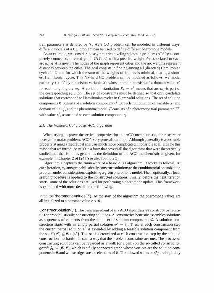
the problem instance tackled. For example, the pheromone update rule from Eq. (2), oncewritten in HCF-form, becomes

�ji ← (1 − �) · �ji + � · ∑{s∈Supd|cji ∈s}

F(s)∑{s′∈Supd} F(s

′), (8)

for i = 1, . . . , n, j = 1, . . . , |Di |. The difference between this pheromone update rule andthe one that is used in standard ACO algorithms consists in the normalization of the addedamount of pheromone.

In order to give a graphical interpretation of the pheromone update in the HCF, we considera solutions from a different point of view. With respect to a solutions ∈ S, we partitionthe set of solution componentsC into two subsets, the setCin that contains all solutioncomponentscji ∈ s, andCout = C \ Cin. In this way, we can associate to a solutions abinary vector�s of dimension|C| in which the position corresponding to solution componentcji is set to 1 ifcji ∈ Cin, to 0 otherwise. This means that we can regard a solutions as a

corner of the|C|-dimensional unit hyper-cube, and that the set of feasible solutionsS canbe regarded as a (sub)set of the corners of this same hypercube. In the following, we denotethe convex hull ofS by S. It holds that

�� ∈ S ⇔ �� = ∑s∈S

�s�s, �s ∈ [0,1], ∑s∈S

�s = 1. (9)

As an example see Fig.1(a). In the following, we give a graphical interpretation of thepheromone update rule in the HCF. When written in vector form, Eq. (8) can be expressedas

�� ← (1 − �) · �� + � · �m, (10)

where �m is a|C|-dimensional vector with

�m = ∑s∈Supd

s · �s wheres = F(s)∑s′∈Supd

F(s′). (11)

Vector �m is a vector inS, the convex hull ofS, as∑s∈Siter

s = 1 and 0�s�1∀ s ∈ Siter.It also holds that vector�m is the weighted average of binary solution vectors. The higherthe qualityF(s) of a solutions, the higher its influence on vector�m. Simple algebra allowsus to express Eq. (10) as

�� ← �� + � · ( �m − ��). (12)

This shows that the application of the pheromone update rule in the HCF shifts the currentpheromone value vector�� toward �m (see Fig.1(b)). The size of this shift is determinedby the value of parameter�. In the extreme cases there is either very little update (when� is very close to zero), or the current pheromone value vector�� is replaced by�m (when� = 1). Furthermore, if the initial pheromone value vector�� is in S, it remains inS,and the pheromone values are bounded to the interval[0,1]. This means that the HCF,


(0, 1, 1) (1, 1, 1) (0, 1, 1) (1, 1, 1)

(1, 0, 1) (0, 0, 1)(0, 0, 1)

(0, 0, 0) (1, 0, 0) (0, 0, 0) (1, 0, 0)

(1, 1, 0) (1, 1, 0)

(1, 0, 1)

Sol. of ant 1

Sol. of ant 2

(a) (b)

Fig. 1. (a) Example of the convex hull of binary solution vectors; (b) example of the pheromone update in theHCF. In this example, the setS of feasible solutions in binary vector form consists of the three vectors(0,0,0),(1,1,0) and(0,1,1). The gray shaded area depicts the setS. In (b), two solutions have been created by twoants. The vector�m is the weighted average of these two solutions (where we assume that(0,0,0) is of higherquality), and�� will be shifted toward�m as a result of the pheromone value update rule (Eq. (8)). Figure from[6].© IEEE Press.

independently of the problem instance tackled, defines the hyper-space for the pheromonevalues to be the|C|-dimensional unit hypercube.10

It is interesting to note that in the case of the IB- and BS-update rules (in which only onesolutionsupd ∈ {sib, sbs} is used for updating) the old pheromone vector�� is shifted towardthe updating solutionsupd in binary vector form:

�� ← �� + � · (�supd − ��). (13)

As a notational convention we use HCF-AS-update, HCF-IB-update, and HCF-BS-update,if the corresponding update rules are considered for an ACO algorithm that is implementedin the HCF.

2.4. Models of ACO algorithms

Merkle and Middendorf introduced the use of models of ACO algorithms in[49] for thestudy of the dynamics of the ACO algorithm search process. A model of an ACO algorithmis a deterministic dynamical system obtained by applying the expected pheromone updateinstead of the real pheromone update. The advantage of studying an ACO algorithm modelis that it—being deterministic—behaves always in the same way, in contrast to the behaviorof the ACO algorithm itself which in each run slightly differs due to the stochasticity. Thereare several ways of studying an ACO model. For example, one might study the evolution ofthe pheromone values over time, or one might study the evolution of the expected quality of

10 Note that earlier attempts to normalize pheromone values exist in the literature (see, for example,[35]).However, existing approaches do not provide a framework for doing it automatically.


the solutions that are generated per iteration. This expected iteration quality is henceforthdenoted byWF(T ), or byWF(T | t), wheret > 0 is the iteration counter.

We use the following notation for defining ACO models. The template for thisnotation is

M(< problem>,< update_rule>,< nr_of_ants>), (14)

where< problem> is the considered problem (or problem type, such as, for example,unconstrained problems),< update_rule> is the pheromone update rule that is considered,and< nr_of_ants> is the number of ants that build solutions at each iteration. The number< nr_of_ants> can be a specific integerna�1, any finite integer (denoted byna < ∞), orna = ∞. In all cases, the character∗ denotes any possible entry. As an example, considerthe modelM(∗,AS, na < ∞): this is the model of an ACO algorithm that can be applied toany problem, and that uses the AS-update rule and a finite number of ants at each iteration.The expected iteration quality of modelM(∗,AS, na < ∞) is

WF(T ) = ∑Sna∈Sna

(p(Sna | T ) · 1

na· ∑s∈Sna

F (s)

), (15)

whereSna is the set of all multi-sets of cardinalityna consisting of elements fromS, andp(Sna | T ) is the probability that thena ants produce the multi-setSna ∈ Sna , given thecurrent pheromone values. The expected pheromone update of modelM(∗,AS, na < ∞)

is

�ji ← (1 − �) · �ji + �

na· ∑Sna∈Sna

p(Sna | T )

∑s∈Sna |cji ∈s

F(s)

, (16)

for i = 1, . . . , n, j = 1, . . . , |Di |.In order to reduce the computational complexity we may consider modelM(∗,AS, na =

∞), which assumes an infinite number of ants per iteration.11 In this case, the expectediteration quality is given by

WF(T ) = ∑s∈S

F(s) · p(s | T ), (17)

wherep(s | T ) is the probability to produce solutions given the current pheromone values.The expected pheromone update of modelM(∗,AS, na = ∞) is given by

�ji ← (1 − �) · �ji + � · ∑{s∈S|cji ∈s}

F(s) · p(s | T ). (18)

If, instead, we consider modelM(∗,HCF-AS, na = ∞), that is, the AS algorithm im-plemented in the HCF using an infinite number of ants, the expected iteration quality isthe same as in modelM(∗,AS, na = ∞) (see Eq. (17)), but the expected pheromone

11 The way of examining the expected behavior of an algorithm by assuming an infinite number of solutions periteration has already been used in the field of evolutionary computation (see for example thezeroth order modelproposed in[57]).


update becomes

�ji ← (1 − �) · �ji + � · ∑{s∈S|cji ∈s}

F(s)·p(s|T )WF (T )

, (19)

for i = 1, . . . , n, j = 1, . . . , |Di |. The study of models of ACO algorithms will play animportant role in Section5 of this paper.

3. Convergence of ACO algorithms

In this section, we discuss convergence of two classes of ACO algorithms: ACObs,�min

and ACObs,�min(t). These two classes are defined as follows. First, in order to ease thederivations, both ACObs,�min and ACObs,�min(t) use simplified transition probabilities thatdo not consider heuristic information: Eq. (1) (see Section 2.1), becomes

p(cji | sp) = [�ji ]�

∑clk∈N(sp) [�

lk]�

, ∀ cji ∈ N(sp). (20)

Second, both algorithm classes use the BS-update rule (see Section2.2). Third, bothACObs,�min and ACObs,�min(t) use a lower limit�min > 0 for the value of pheromone trails,chosen so that�min < F(s∗), wheres∗ is an optimal solution. ACObs,�min(t) differs fromACObs,�min because it allows the change of the value of�min at run-time.

For ACObs,�min convergence in value is proven via Theorem 1 which essentially says that,because of the use of a fixed positive lower bound on the pheromone values, ACObs,�min isguaranteed to find an optimal solution if given enough time.

For ACObs,�min(t), first convergence in value is proven via Theorem 2, under the conditionthat the bound�min decreases to zero slowly enough.12 Then, convergence in solutionis proven via Theorem 3, which shows that a sufficiently slow decrement of the lowerpheromone trail limits leads to the effect that the algorithm converges to a state in which allthe ants construct the optimal solution over and over again (made possible by the fact thatthe pheromone trails go to zero).

3.1. Convergence in value

In this subsection, we state that ACObs,�min is guaranteed to find an optimal solution witha probability that can be made arbitrarily close to 1 if given enough time (convergencein value). However, as we will indicate in Section 3.2, the convergence in solution forACObs,�min cannot be proved.

In Proposition 1 (see Section 2.2) it was proved that, due to pheromone evaporation,the pheromone values are asymptotically bounded from above with�max as the limit. Thefollowing proposition follows directly from Proposition 1.

12 Unfortunately, Theorem2 cannot be proven for the exponentially fast decrement of the pheromone trailsobtained by a constant pheromone evaporation rate, which most ACO algorithms use.


Proposition 2. Once an optimal solutions∗ has been found by algorithm ACObs,�min, itholds that

∀cji ∈ s∗ : limt→∞ �ji (t) = �max = F(s∗)

�. (21)

The proof of this proposition is basically a repetition of the proof of Proposition1,restricted to the solution components of the optimal solutions∗. Additionally, �0 has—foreach cji ∈ s∗—to be replaced by�ji (t

∗) (where t∗ is the iteration in whichs∗was found).

Proposition 1 implies that, for the proof of Theorem 1 (see below), the only essentialpoint is that�min > 0, because from above the pheromone values will anyway be boundedby �max. Proposition 2 additionally states that, once an optimal solutions∗ has been found,the pheromone values on all solution components ofs∗ converge to�max = F(s∗)/�.

Theorem 1. Letp∗(t) be the probability that ACObs,�min finds an optimal solution at leastonce within the first t iterations. Then, for an arbitrarily small� > 0 and for a sufficientlylarge t it holds that

p∗(t)�1 − �, (22)

and asymptoticallylim t→∞ p∗(t) = 1.

Proof. The proof of this theorem consists in showing that, because of�min > 0, at eachalgorithm iteration any generic solution, including any optimal solution, can be generatedwith a probability greater than zero. Therefore, by choosing a sufficiently large number ofiterations, the probability of generating any solution, and in particular an optimal one, canbe made arbitrarily close to 1. For a detailed proof see[65] or [24]. �

3.2. Convergence in solution

In this subsection we deal with the convergence in solution of algorithm ACObs,�min(t).For proving this property, it has to be shown that, in the limit, any arbitrary ant of the colonywill construct the optimal solution with probability one. This cannot be proven if, as done inACObs,�min, a small, positive lower bound is imposed on the lower pheromone value limitsbecause in this case at any iterationt each ant can construct any solution with a non-zeroprobability. The key of the proof is therefore to allow the lower pheromone trail limits todecrease over time toward zero, but making this decrement slow enough to guarantee thatthe optimal solution is eventually found.

The proof of convergence in solution as presented in [24] was inspired by an earlier workof Gutjahr [38]. It is organized in two theorems. First, Theorem 2 proves convergence invalue of ACObs,�min(t) when its lower pheromone trail limits decrease toward zero at not morethan logarithmic speed. Next, Theorem 3 states, under the same conditions, convergence insolution of ACObs,�min(t).


Theorem 2. Let the lower pheromone trail limits in ACObs,�min(t) be

∀t�1, �min(t) = d

ln(t + 1), (23)

with d being a constant, and letp∗(t) be the probability that ACObs,�min(t) finds an optimalsolution at least once within the first t iterations. Then it holds that

limt→∞ p∗(t) = 1. (24)

Proof. The proof consists in showing that there is an upper bound to the probability of notconstructing an optimal solution whose value goes to zero in the limit. A detailed proof canbe found in[24]. �

It remains to be proved that any ant will in the limit construct the optimal solution withprobability 1 (i.e., convergence in solution). This result is stated in Theorem 3.

Theorem 3. Let t∗ be the iteration in which the first optimal solutions∗ has been foundandp(s∗, t, k) be the probability that an arbitrary ant k constructss∗ in the t-th iteration,with t > t∗. Then it holds thatlim t→∞ p(s∗, t, k) = 1.

Proof. The proof of this theorem consists in showing that the pheromone values of solutioncomponents that do not belong to the optimal solution asymptotically converge to 0. Fordetails see[24]. �

3.3. Extension to include additional features of ACO algorithms

Most, if not all, ACO algorithms in practice include some features that are present neitherin ACObs,�min nor in ACObs,�min(t). Of particular interest is how the use of local search toimprove the constructed solutions and the use of heuristic information affect the convergenceproof for ACObs,�min. 13 Concerning the use of local search, it is rather easy to see that itneither affects the convergence properties of ACObs,�min, nor those of ACObs,�min(t). This isbecause the validity of both convergence proofs (as presented in [24]) depends only on theway solutions are constructed and not on the fact that the solutions are taken or not to theirlocal optima by a local search routine.

The second question concerns the consequences of the use of heuristic information, thatis, when considering Eq. (1) instead of Eq. (20) for computing the transition probabilitiesduring solution construction. In fact, neither Theorem 1 nor Theorems 2 and 3 are affectedby the heuristic information, if we have 0< �(cji ) < +∞ for eachcji ∈ C and� < ∞. Infact, with these assumptions�(·) is limited to some (instance specific) interval[�min, �max],with �min > 0 and�max < +∞. Then, the heuristic information has the only effect to changethe lower bounds on the probability of making a specific decision (which is an importantcomponent of the proofs of Theorems 2 and 3).

13 Note that, here and in the following, although the remarks made on ACObs,�minin general also apply to

ACObs,�min(t), for simplicity we often refer only to ACObs,�min

.


3.4. Convergence proofs for other types of ACO algorithms

A pioneering study from which much of the inspiration for later works was taken isthat of Gutjahr[36–38]. In [37] he presented the first piece of research on the convergenceproperties of ACO algorithms, which deals with the convergence in solution for the so-called graph-based ant system (GBAS). GBAS is very similar to ACObs,�min(t) except that�min = 0 and the pheromone update rule changes the pheromones only when, in the currentiteration, a solution at least as good as the best one found so far is generated. The followingtheorems were proved for GBAS:

Theorem 4. For each� > 0, for a fixed evaporation rate�, and for a sufficiently largenumber of ants, the probabilityp that a fixed ant constructs the optimal solution at iterationt is p�1 − � for all t� t0, with t0 = t0(�).

Theorem 5. For each� > 0, for a fixed number of ants, and for an evaporation rate�sufficiently close to zero, the probabilityp that a fixed ant constructs the optimal solutionat iteration t isp�1 − � for all t� t0, with t0 = t0(�).

One of the limitations of these proofs is that they require the problem to have a singleoptimal solution. This limitation has been removed in an extension of the above two resultsin [36]. Another limitation is the way of updating the pheromone values. While the conver-gence results presented in previous sections hold independently of the way the pheromonevalues are updated, the theorems for GBAS hold only for its particular pheromone updaterule. In [36] this limitation was weakened by only requiring the GBAS update rule in thefinal phases of the algorithm.

Finally, Gutjahr [38] provided a proof of convergence in solution for two variants ofGBAS that gave the inspiration for the proof of Theorem 2. The first variant was calledGBAS/tdlb (for time-dependent lower pheromone bound), and the second one GBAS/tdev(for time-dependent evaporation rate). GBAS/tdlb uses a lower bound on the pheromonevalues very similar to the one that is used in Theorem 2. Differently, in GBAS/tdev it is thepheromone evaporation rate that is varied during the run of the algorithm: for proving thatGBAS/tdev converges in solution, pheromone evaporation is decreased slowly, and in thelimit it tends to zero.

3.5. Final remarks on convergence proofs

From the point of view of the researcher interested in practical applications of the al-gorithms, the interesting part of the discussed convergence proofs is Theorem 1, whichguarantees that ACObs,�min will find an optimal solution if it runs long enough. It is there-fore interesting that this theorem also applies to ACO algorithms that differ from ACObs,�min

in the way the pheromone update procedure is implemented. In general, Theorem 1 appliesto any ACO algorithm for which the probabilityp(s) of constructing a solutions ∈ S

always remains greater than a small constant� > 0. In ACObs,�min this is a direct conse-quence of the fact that 0< �min < �max < +∞, which was obtained by (i) explicitly settinga minimum value�min for pheromone trails, (ii) limiting the amount of pheromone that the


ants may deposit after each iteration to finite values, (iii) letting pheromone evaporate overtime, that is, by setting� > 0, and by (iv) the particular form of choosing the transitionprobabilities. As mentioned in Section2.2, we call the class of ACO algorithms that imposea lower bound (and, implicitly, an upper bound) to the pheromone values ACO�min. By defi-nition, Theorem 1 holds therefore for any algorithm in ACO�min, which contains practicallyrelevant algorithms such as ACS andMMAS.

Open problem 1. The proofs that were presented in this section do not say anything aboutthe time required to find an optimal solution, which can be astronomically large. It wouldbe interesting to obtain results on convergence speed for ACO algorithms, in spirit similarto what has been done in evolutionary computation for relatively simple problems such as,for example, ONE-MAX[43].

4. Model-based search

Up to now we have regarded ACO algorithms as a class of stochastic search proceduresworking in the space of the solutions of a combinatorial optimization problem. Under thisinterpretation, artificial ants are stochastic constructive heuristics that build better and bettersolutions to a combinatorial optimization problem by using and updating pheromone trails.In other words, our attention has been directed to the stochastic constructive procedure usedby the ants and to how the ants use the solutions they build to bias the search of future ants bychanging pheromone values. In the following, we show that by changing the point of view,we can clarify the intrinsic relation of ACO algorithms to algorithms such as stochasticgradient ascent (SGA) [53,60] and the cross-entropy (CE) method [15,61]. This is doneby studying these algorithms under a common algorithmic framework called model-basedsearch (MBS) [67]. The results presented in this section were obtained in [25,52,67].

An MBS algorithm is characterized by the use of a (parametrized) probabilistic modelM ∈ M (whereM is the set of all possible probabilistic models) that is used to generatesolutions to the problem under consideration. At a very general level, a model-based searchalgorithm attempts to solve an optimization problem by repeating the following two steps:• Candidate solutions are constructed using some parametrized probabilistic model, that

is, a parametrized probability distribution over the solution space.• Candidate solutions are evaluated and then used to modify the probabilistic model in

a way that is deemed to bias future sampling toward low cost solutions. Note that themodel’s structure may be fixed in advance, with solely the model’s parameter values beingupdated, or alternatively, the structure of the model may be allowed to change as well.

In the following, we focus on the use of fixed model structures based on a vector of modelparametersT , and identify a modelMwith its vector of parametersT . The way of samplingsolutions (i.e., the way of constructing solutions) induces a probability functionp( · | T ) onthe search space of the tackled optimization problem. Given this probability function and acertain setting� of the parameter values, the probability of a solutions ∈ S to be sampledis denoted byp(s | �). We assume that• ∀ s ∈ S the model parameters can assume values�s such that the distributionp( · | �s)

defined byp(s | �s) = 1 andp(s′ | �s) = 0 ∀ s′ �= s is obtained. This “expressiveness”


assumption is needed in order to guarantee that the sampling can concentrate in theproximity of any solution, an optimal solution in particular;14

• and that the probability functionp( · | T ) is continuously differentiable with respectto T .

In MBS algorithms, the view on an algorithm is dominated by its probabilistic model.Therefore, the tackled optimization problem is replaced by the following continuous max-imization problem:

�∗ ← argmax�

WF(T ), (25)

whereWF(T ) (as introduced in Section2.4) denotes the expected quality of a generatedsolution depending on the values of the parametersT . It may be easily verified that,under the “expressiveness’’ assumption we made about the space of possible probabilitydistributions, the support ofp( · | �∗) (i.e., the set{s | p(s | �∗) > 0}) is necessarilycontained inS∗. This implies that solving the problem given by Eq. (25) is equivalent tosolving the original combinatorial optimization problem.

In the following we first outline the SGA and the CE methods in the MBS framework,before we show the relation of the two methods to ACO algorithms. In particular, we willsee that the pheromone update rules as proposed in the ACO literature have a theoreticaljustification.

4.1. Stochastic gradient ascent

A possible way of searching for a (possibly local) optimum of the problem given byEq. (25) is to use the gradient ascent method. In other words, gradient ascent may beused as a heuristic to change� with the goal of solving Eq. (25). The gradient ascentprocedure starts from some initial model parameter value setting� (possibly randomlygenerated). Then, at each iteration it calculates the gradient∇WF(T ) and updates� tobecome� + �∇ WF(T )|�, 15 where� is a step-size parameter.

The gradient can be calculated (bearing in mind that∇ ln f = ∇f/f ) as follows:

∇WF(T )= ∇ ∑s∈S

F(s)p(s | T ) = ∑s∈S

F(s)∇p(s | T )

= ∑s∈S

p(s | T )F (s)∇p(s|T )p(s|T )

= ∑s∈S

p(s | T )F (s)∇ ln p(s | T ). (26)

However, the gradient ascent algorithm cannot be implemented in practice, as for its eval-uation a summation over the whole search space is needed. A more practical alternative isthe use ofstochastic gradient ascent, which replaces—for a given parameter setting�—the expectation in Eq. (26) by an empirical mean of a sample generated fromp( · | �).

14 Note that this condition may be relaxed by assuming that the probability distribution induced by a parametervalue setting� is in the closure of all inducible probability distributions.

15 Note that∇WF (T )|� denotes the gradient ofWF (T ) evaluated in�.


The update rule for the stochastic gradient then becomes

�(t + 1) = �(t) + �∑

s∈Supd

F(s)∇ ln p(s | �(t)), (27)

whereSupd is the sample at iterationt. In order to derive a practical algorithm from theSGA approach, we need a model for which the derivatives of lnp( · | T ) can be calculatedefficiently. In Section4.3 we will show how this can be done within the context of the ACOmetaheuristic.

4.2. The cross-entropy method

Starting from some initial distribution that is given by the probability functionp( · | �(0))(denoted in the following byp0), the CE method inductively builds a series of distributionspt = p( · | �(t)) in an attempt to increase the probability of generating high quality solutionsafter each iteration. A tentative way to achieve this goal is to setpt+1 equal top, wherepis proportional topt as follows:

p ∝ ptF (·), (28)

whereF(·) is, again, some quality function, depending on the objective function.If this were possible, then, for time independent quality functions, aftert iterations we

would obtainpt ∝ p0F(·)t . Consequently, ast → ∞, pt would converge to a probabilitydistribution restricted toS∗. Unfortunately, even if the distributionpt is such that it canbe induced by some setting� of the parameter values, for the distributionp as definedby Eq. (28) this does not necessarily hold, hence some sort of projection is needed. Anatural candidate for the projectionpt+1 is the distributionp that minimizes theKullback–Leibler divergence[45], which is a commonly used measure of the difference between twodistributions:

D(p‖p) = ∑s∈S

p(s | T ) lnp(s | T )

p(s | T )(29)

or equivalently thecross-entropy:

− ∑s∈S

p(s | T ) ln p(s | T ). (30)

Sincep ∝ ptF (·), the cross-entropy minimization is equivalent to the following maximiza-tion problem:

pt+1 = argmaxp(·|�)

∑s∈S

p(s | �(t))F (s) ln p(s | �). (31)

In a way similar to what happened with the gradient of Eq. (26), the maximization problemgiven by Eq. (31) cannot be solved in practice, because the evaluation of the function onthe right-hand side requires summation over the whole search space. As before, however,a finite sample approximation can be used

pt+1 = argmaxp(·|�)

∑s∈Supd

F(s) ln p(s | �), (32)


whereSupd is the sample at iterationt. In some relatively simple cases this problem canbe solved exactly. In general, however, the analytical solution is unavailable. Still, even ifthe exact solution is not known, some iterative methods such as SGA for solving this opti-mization problem may be used. It should be noted that, since the new vector of pheromonevalues�(t + 1) is a random variable, depending on a sample, there is no use in runningthe SGA process till full convergence. Instead, in order to obtain some robustness againstsampling noise, a fixed number of SGA updates may be used. One particular choice, whichis of special interest, is the use of a single gradient ascent update, leading to an updaterule which is identical to the SGA update shown in Eq. (27). However, in general the CEmethod imposes less restrictions on the quality function (e.g., allowing it to change overtime), hence the resulting algorithm may be seen as a generalization of SGA.

4.3. Relation of ACO with SGA and the CE method

The discussion of SGA and of the CE method in the previous two sections was focusedon the update of the model parameter values. However, this is only one of the componentsneeded in any model-based search algorithm. In the following we focus on the probabilityfunction p( · | T ) that is implicitly given by the solution construction process of ACOalgorithms. We show that the calculation of the derivatives of this probability function canbe carried out in a reasonable time, and we outline the existing work on deriving updatesof the parameter values that describe a SGA, respectively a CE method, in the space of theparameter values.

TheSGAupdate inACO.The SGA parameter value update that we describe in the followingis a generalization of the one that was presented in [67] (which was itself a generalizationof the one that was given in [52]).

As described in Section 2.1, in ACO algorithms a solutions is constructed as a finite-length sequence〈cji , . . . , clk, . . . , csr 〉 of solution componentsc from the setC of solu-tion components. For the sake of simplicity, we rename the components of the sequenceso to obtain〈c1, c2, . . . , c|s|〉. By defining the transition probabilities as done in Eq. (1)(see p. 8), the probability function in ACO algorithms can be written as

p(s | T ) =|s|−1∏h=1

p(ch+1 | sph), (33)

wheresph is the partial sequence〈c1, . . . , ch〉, and consequently

∇ ln p(s | T ) =|s|−1∑h=1

∇ ln p(ch+1 | sph). (34)

Let us now consider an arbitrary solution construction steph ∈ {1, . . . , |s|} with N(sph)being the set of solution components that can be added to the current partial sequences

ph .

For the sake of readability let us also denote the “desirability’’[�ji ]� · [�(cji )]

�of a solution

componentcji (as used for determining the transition probabilities in Eq. (1)) by d(cji ).


If cji ∈ N(sph) andcji = ch+1 it holds that

�

�T ji

{ln p(cji | sph)

}= �

�T ji

ln

(d(cji )

/ ∑clk∈N(sph )

d(clk)

)

= �

�T ji

{ln d(cji ) − ln

∑clk∈N(sph )

d(clk)

}

= d′(cji )/

d(cji ) − d′(cji )/ ∑clk∈N(sph )

d(clk)

=1 − d(cji )

/ ∑clk∈N(sph )

d(clk)

d′(cji )

d(cji )

={

1 − p(cji | sph)}

d′(cji )d(cji )

. (35)

Otherwise, ifcji ∈ N(sph) but cji �= ch+1 it holds (by a similar argument) that

�

�T ji

{ln p(cji | sph)

}= −p(cji | sph)

d′(cji )d(cji )

. (36)

Finally, if cji /∈ N(sph) thenp(cji | sph) is independent ofT ji and therefore we have that

�

�T ji

{ln p(cji | sph)

}= 0. (37)

By combining these results, the SGA pheromone update procedure is derived as follows.Let s be the solution for which pheromone updates have to be performed. First, because ofEqs. (27) and (35), pheromones associated to solution componentsc

ji ∈ sare reinforced with

the amount�F(s) ·d′(cji )/d(cji ). Then, because of Eqs. (27), (35) and (36), pheromones that

are associated to all the solution components that were considered16 during the constructionof s are decreased by an amount given by�F(s) · p(cji | sph) · d′(cji )/d(c

ji ). Last, because

of Eq. (37), all the remaining pheromones are not updated.In order to guarantee stability of the resulting algorithm, it is desirable to have a bounded

gradient∇ ln p(s | T ). This means that a function d(·), for which d′(·)/d(·) is bounded,should be used. In [52] the authors suggest using d(·) = exp(·), which leads to d′(·)/d(·) ≡1. It should be further noted that if, in addition,F(·) = 1/f (·) and� = 1, the reinforcementpart becomes 1/f (·) as in the original Ant System algorithm (see Section 2.2).

The cross-entropy update inACO.As we have shown in Section 4.2, the CE method requiresat each step the solution of the problem stated in Eq. (32). Since, in general, the exact solutionis not available, an iterative scheme such as gradient ascent could be employed. As we haveshown in the previous section, the gradient of the log-probability for ACO-type probabilisticfunctions can be efficiently calculated. The obtained values may be plugged into any general

16 We say that a solution componentcji

was “considered’’ at construction steph, if cji

∈ N(sph).


iterative solution scheme of the cross-entropy minimization problem, for example, the onedescribed by Eq. (27). If, for example, we use a single-step gradient ascent for solvingEq. (32), we obtain a generalization of the SGA pheromone update, in which the qualityfunction is permitted to change over time.

In some special cases, such as for example unconstrained problems, it can be shown(see [24]) that the parameter update of the CE method is exactly the same as the update ofAnt System implemented in the HCF (see Section 2.3) with a setting of� = 1 (rememberthat� is the evaporation rate in standard ACO update rules).

Open problem 2. The relation of ACO algorithms to other probabilistic learning algo-rithms such as estimation of distribution algorithms[55],or graphicalmodels andBayesiannetworks[42], is relatively unexplored. More work on these subjects could be of interest.

5. Search bias in ACO algorithms

In ACO algorithms we find different forms of search bias. A first type of desirablebias, whose goal is to direct the search towards good zones of the search space, is givenby the pheromone update rule. A less desirable form of bias, however, can be caused byalgorithm features such as the pheromone model and the solution construction process.In fact, sometimes this additional bias is harmful and results in a decrease of algorithmperformance over time. There are basically two different strands of work on this type ofpotentially harmful bias in ACO algorithms. In this section we first review results obtainedby Blum et al. in [12,7], and then we summarize those obtained by Merkle and Middendorfin [49].

5.1. Negative search bias caused by an unfair competition

The fact that the average quality of the generated solutions improves over time is, ingeneral, considered to be a desirable characteristic for a metaheuristic. This is becausethe generation of better average quality solutions during the algorithms’ execution is oftenpositively correlated with the probability to generate improved best solutions. Therefore,situations in which this is not the case might be labelednegative search bias, as it was doneby Blum and Dorigo in [7]. For detecting this type of search bias, they studied the evolutionof the expected iteration qualityWF(T | t) 17 of the solutions that are generated by ACOalgorithm models.

First, the application of ACO algorithms to unconstrained CO problems was consid-ered, that is, CO problems in which the set� of constraints is empty (see Definition 1at p. 6). By relating the expected pheromone update to a type of function calledgrowthtransformation[1], the following result was proved in [6]:

Theorem 6. The expected iteration qualityWF(T ) ofM(U,HCF-AS, na = ∞), whereU stands for the application to unconstrained problems, is continuously non-decreasing.

17WF (T | t) is the value ofWF (T ) at iterationt. For a definition ofWF (T ) see Section2.4.


More formally, it holds that

WF(T | t + 1) > WF (T | t), (38)

as long as at least one pheromone value changes from iteration t to iterationt + 1.

An extension of this result to the modelM(U,AS, na = ∞) was later presented in[5].These results indicate that the AS algorithm shows a desired behavior when applied tounconstrained problems. However, this result is not exceedingly useful, because most of therelevant optimization problems tackled with ACO algorithms are constrained. Therefore, thefocus of research shifted to constrained problems. An example is the case study concerningthe NP-hardk-cardinality tree (KCT) problem [12,3], a generalization of the well-knownminimum spanning tree (MST) problem. It is defined as follows: Given is an undirectedgraphG = (V ,E) (where|V | = n and|E| = m) with edge-weightsw(e) ∈ N+, ∀ e ∈ E.The set of all trees inG with exactlyk edges is henceforth denoted byTk. The goal is tofind a treeTk ∈ Tk that minimizes

f (Tk) = ∑e∈E(Tk)

w(e). (39)

This means that the objective function value of ak-cardinality tree is given by the sumof the weights of all its edges. We consider the following CO problem model of the KCTproblem: We assign a binary decision variableXe to each edgee ∈ E. If Xe = 1, thene ispart of thek-cardinality tree that is built. The pheromone model is derived as follows. Weintroduce for each of the binary decision variablesXe two solution components:c0

e , whichcorresponds toXe = 0, andc1

e corresponding toXe = 1. The pheromone model consists

of a pheromone trail parameterT je for each solution componentcje , with j ∈ {0,1}.

The considered solution construction mechanism works as follows. The algorithm startswith an empty partial solutionsp0 = 〈〉, and with empty setsET (for collecting the addededges) andVT (for collecting the implicitly added vertices). Then, at construction steph,0 < h < k, a solution componentc1e ∈ N(sph) is added to the current partial solutionsph .When adding the solution componentc1e to sph we also adde = {v, v′} toET andv andv′ toVT . For the first construction step, setN(sp0 ) is defined asN(sp0 ) = {c1e | e = {v, v′} ∈ E}and for each subsequent construction steph as

N(sph) = {c1e | (e = {v, v′} ∈ E \ ET ) ∧ ((v ∈ VT ) ∨ (v′ ∈ VT ))}. (40)

The definition ofN(sph) is such that only feasiblek-cardinality trees can be generated.After k construction steps are performed we add, for alle ∈ E with c1e /∈ s

pk , the solu-

tion componentc0e to spk . By this last step a sequences is completed that corresponds toa feasible solution. The transition probabilities are at each construction step defined byEq. (1), with � = 1 and� = 0. The setting of� = 0 means that no heuristic infor-mation for biasing the transition probabilities was considered in order to study the purebehavior of the algorithm.


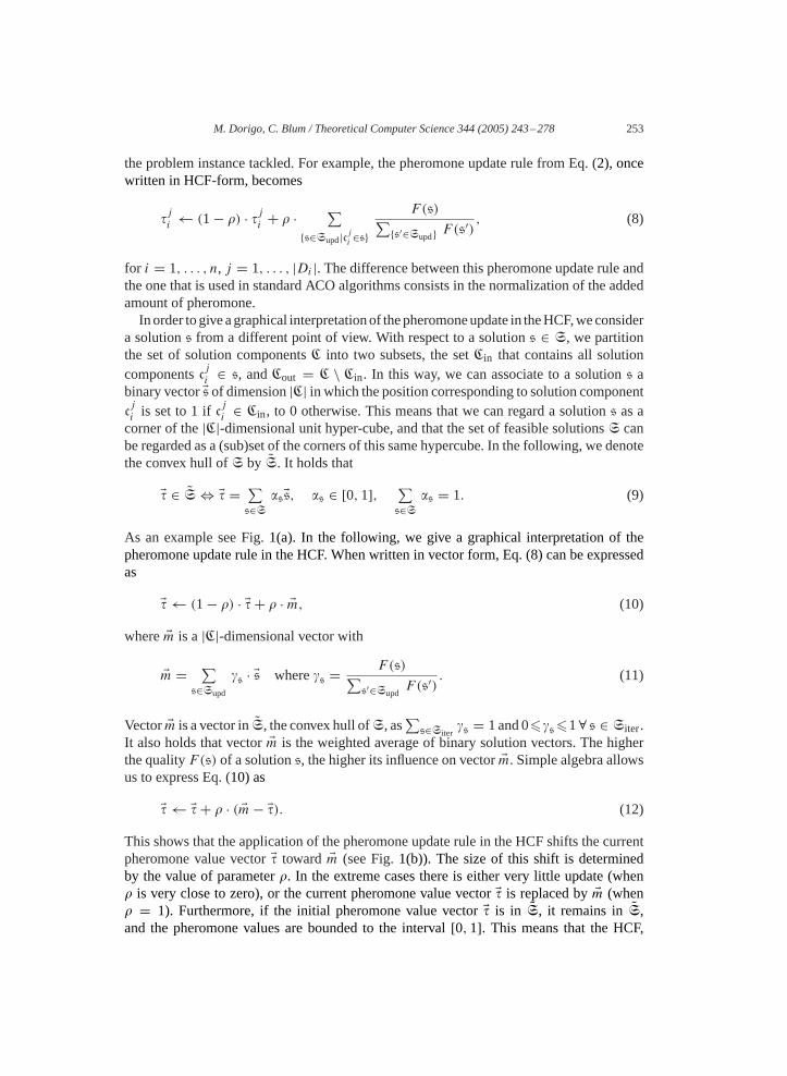
Fig. 2. The complete search tree defined by the solution construction mechanism of the ACO algorithm and theproblem instancekct_simple_inst. The bold path in the search tree shows the steps of constructing solutions3 = 〈c1e2

, c1e3, c0e1

, c0e4〉. Figure from[3]. © Akademische Verlagsgesellschaft Aka GmbH.

The evolution of the modelM(KCT,AS, na = ∞) and the behavior of the AS algorithmwas studied when applied to the following small problem instance:

The weight settings for this instance arew(e1) = w(e4) = 1 andw(e2) = w(e3) = 2.Let us denote this problem instance bykct_simple_inst, and let us consider the problemof solving the 2-cardinality tree problem inkct_simple_inst. An ACO algorithm usingthe above described solution construction mechanism can produce six different sequencesof solution components that map to valid solutions. All six possible solution constructionsare shown in form of a search tree in Fig.2, where sequencess1 ands2 correspond to thesolution(1,1,0,0), that is,(X1 = 1, X2 = 1, X3 = 0, X4 = 0), s3 ands4 correspond tothe solution(0,1,1,0), ands5 ands6 map to the solution(0,0,1,1). The objective functionvalues aref (s1) = f (s2) = f (s5) = f (s6) = 3 andf (s3) = f (s4) = 4. This meansthats1, s2, s5, ands6 are optimal solutions to this problem instance, whereass3 ands4 aresub-optimal solutions.

The results of applying the modelM(KCT,AS, na = ∞) to kct_simple_inst are graph-ically shown in Fig. 3. The expected iteration qualityWF continuously decreases over time.At first sight, this is a surprising result, as we would expect the exact opposite from anACO algorithm. However, this behavior can be easily explained by taking a closer look atthe search tree that is shown in Fig. 2. In the first construction step, there are four differ-ent possibilities to extend the empty partial solution. The four solution components thatcan be added arec1e1

, c1e2, c1e3

, andc1e4. However, solution componentsc1e1

and c1e4in ex-

pectation only receive update from two solutions (i.e., sequencess1 ands2 in case ofc1e1,

respectively sequencess5 ands6 in case ofc1e4), whereas solution componentsc1e2

andc1e3in expectation receive update from four solutions (i.e., sequencessi , wherei ∈ {1, . . . ,4},in case ofc1e2

, respectively sequencessi , wherei ∈ {3, . . . ,6}, in case ofc1e3). This means

that for many initial settings of the pheromone values (e.g., when the initial pheromonevalues are set to the same positive constantc > 0) T 1

e2and T 1

e3receive in expectation


0.27

0.28

0.29

0.3

0.31

0.32

0.33

0.34

0.35

0 500 1000 1500 2000

expe

cted

qua

lity

iteration

ρ = 0.01ρ = 0.05

ρ = 0.1ρ = 0.5

Fig. 3. The evolution of the expected iteration qualityWF of the modelM(KCT,AS, na = ∞) applied toproblem instancekct_simple_inst for different settings of the evaporation parameter�. All the pheromone valueswere initialized to 0.5. The plots show that the expected iteration quality continuously decreases. Moreover, forincreasing� the impact of the pheromone value update increases and the expected iteration quality decreasesfaster. Figure from[3]. © Akademische Verlagsgesellschaft Aka GmbH.

more updates thanT 1e1

and T 1e4

just because the number of solutions that contribute totheir updates is higher. Therefore, over time the probability of constructing the sub-optimalsolutionss3 ands4 increases, whereas the probability of constructing the optimal solutionssi , wherei ∈ {1,2,5,6}, decreases. This means that the expected iteration quality decreasesover time.

The behavior of the real AS algorithm was compared to the behavior of its model byapplying AS to the same problem instancekct_simple_inst. Fig. 4 shows the evolutionof the empirically obtained average quality of the solutions per iteration for two differentevaporation rate values. The results show that when� is small the empirical behavior ofthe algorithm approximates quite well the behavior of its model. However, the stochasticerror makes the real AS algorithm, after approximately 1000 iterations, decide for one ofthe two optimal solutions, which results in a turn from decreasing average iteration qualityto increasing average iteration quality.

The bias that is introduced by the fact that some solution components receive in expecta-tion updates from more solutions than others results from an unfair competition between thesolution components. In contrast, a fair competition can be defined as follows (see also [7]):

Definition 2. Given a modelP of a CO problem, we call the combination of an ACOalgorithm and a problem instanceP of P a competition-balanced system(CBS), if thefollowing holds: given a feasible partial solutionsp and the set of solution componentsN(sp) that can be added to extendsp, each solution componentc ∈ N(sp) is a componentof the same number of feasible solutions (in terms of sequences built by the algorithm) as


0.27

0.28

0.29

0.3

0.31

0.32

0.33

0.34

0.35

0.27

0.28

0.29

0.3

0.31

0.32

0.33

0.34

0.35

0 500 1000 1500 2000

aver

age

itera

tion

qual

ity

aver

age

itera

tion

qual

ity

iteration0 500 1000 1500 2000

iteration

AS

AS

(a) (b)

Fig. 4. (a) Instancekct_simple_inst, na = 10,� = 0.01; (b) instancekct_simple_inst, na = 10,� = 0.05. Theplots show the evolution of the average iteration quality obtained by the AS algorithm applied to problem instancekct_simple_inst for na = 10 (i.e., 10 ants per iteration) and two different settings of the evaporation parameter� (� ∈ {0.01,0.05}). All the pheromone values were initialized to 0.5. The results are averaged over 100 runs(error bars show the standard deviation and are plotted every 50-th iteration). Figure from[3]. © AkademischeVerlagsgesellschaft Aka GmbH.

any other solution componentc′ ∈ N(sp), c �= c′. 18 In this context, we call the competitionbetween the solution components afair competitionif the combination of an ACO algorithmand a problem instance is a CBS.

The application to the small KCT example instance has shown that ACO algorithmsapplied to the KCT problem when modeled as shown above are—in general—not CBSs.The question is now if we can expect an algorithmnot to suffer from a negative search biasin case an algorithm/problem instance combination is a CBS. In [7], the authors started toinvestigate this question by studying the application of ACO algorithms to the asymmetrictraveling salesman problem (ATSP). The results of applying the modelM(ATSP,AS, na =∞) to randomly generated ATSP instances suggest that the expected iteration quality iscontinuously non-decreasing. However, in general this question is still open.

Open problem 3. Is the property of being a competition-balanced system sufficient toensure the absence of any negative search bias? In this context, it would be interesting tosee if the result that is stated in Theorem6 can be extended to the modelM(∗, AS, na =∞) applied to problems for which the combination of AS and the problem is a competition-balanced system; as, for example, AS applied to the ATSP.

Finally, we note that a (temporary) decrease in expected iteration quality is not necessarilyan indicator for the existence of a negative search bias. In other words, the evolution ofthe expected iteration quality is not a reliable indicator for negative search bias. As anexample, let us consider the application of the modelM(U, IB, na = ∞) to a very simpleunconstrained maximization problem consisting of two binary variablesX1 andX2. This

18 Note that there exist ACO algorithms in which partial solutions are extended by “groups’’ of solution com-ponents. In these cases the definition of a CBS has to be adapted accordingly.


1.6

1.8

2

2.2

2.4

2.6

2.8

3

0 500 1000 1500 2000

expe

cted

qua

lity

iteration

rho = 0.001

Fig. 5. The evolution of the expected iteration qualityWF of the modelM(U, IB, na = ∞) applied an uncon-strained problem instance with two variables (see text for details).

problem has 4 solutions:s1 = 〈c01, c02〉, s2 = 〈c11, c02〉, s3 = 〈c01, c12〉, ands4 = 〈c11, c12〉.Let us assign the following objective function values:f (s1) = 2, f (s2) = f (s3) = 1,andf (s4) = 3. Note that, as we are maximizing, we chooseF(·) = f (·). Any ACOalgorithm using the solution construction process for unconstrained problems as outlinedat the beginning of this section is a CBS. Let us assume that at the start of the algorithm thepheromone values are initialized so thatp(X1 = 1) = p(X2 = 1) = �, with � a positivenumber close to zero. With this setting, the probability to construct any of the four solutionsis greater than zero. Therefore, as modelM(U, IB, na = ∞) considers an infinite numberof ants per iteration, for sure at each iteration solutions4 will be the iteration-best solution,and will therefore be used for updating the pheromone values. The graphic in Fig.5 showsthe evolution of the expected quality of the solutions generated byM(U, IB, na = ∞)

starting from a setting such that� = 0.01. During the first approximately 200 iterations,the expected quality decreases. For a sufficiently large population size, this result will beapproximated by the IB algorithm. Clearly, in this case, the decrease of expected iterationquality is not due to a negative bias. This leads to another open question:

Open problem 4. Can it be shown that the modelsM(U, IB, na = ∞) and/orM(U,BS,na = ∞) have stable attractors that correspond to solutions to the problems?

5.2. Search bias caused by selection fix-points

Merkle and Middendorf[48–50] studied the dynamics of models of ACO algorithms. Oneof the questions they tackled concerns the source of the driving force of the algorithm. OftenACO practitioners ask themselves: Why to use more than one ant per iteration? Wouldn’tthe algorithm work with only one ant? The work presented in [49] gives a theory-basedanswer to this question. Let us in the following consider the AS algorithm implemented inthe HCF for the application to unconstrained problems; and let us consider the use of one


ant per iteration. The expected pheromone update of the algorithms’ model, that is, modelM(U,AS-HCF, na = 1), 19 is given by

�ji (t + 1) = (1 − �) · �ji (t) + � · ∑{s∈S|cji ∈s}

p(s | T ). (41)

However, it holds that∑

{s∈S|cji ∈s} p(s | T ) = p(cji | T ) (because the tackled problem

is unconstrained). Moreover, it holds thatp(cji | T ) = �ji (t), because the algorithm isimplemented in the HCF. Therefore, Eq. (41) can be rewritten as

�ji (t + 1) = (1 − �) · �ji (t) + � · �ji (t), (42)

and therefore it holds that�ji (t+1) = �ji (t). This means that the expected pheromone updatedoes not change the pheromone values, which shows that—without the competition amongthe ants—in ACO algorithm models applied to unconstrained problems, when consideringeither the AS or the IB updates in the HCF, there is no driving force of the algorithm. Thissuggests that (i) the competition between the ants is a driving force of ACO algorithms,and that (ii) for the above mentioned type of ACO algorithm models, no negative searchbias exists. In the following, we show how this result relates to ACO algorithms that are notimplemented in the HCF.

Let us indicate byji the amount of update that a pheromone value�ji receives. Then,

we can express a general pheromone update rule by

�ji (t + 1) = (1 − �) · �ji (t) + � · ji . (43)

In case of modelM(U,AS, na = 1), it holds that

ji = p(cji | T ) = �ji (t)

/|Di |∑k=1

�ki (t) , (44)

which in general is not equal to�ji (t). Therefore, in case the algorithm is not implemented in

the HCF, Eq. (43) makes the pheromone values move towards a situation in which�ji (t) =ji . Such situations were labeled by Merkle and Middendorfselection fix-pointsin [49],

where they showed the relevance of theselection fix-point biascaused by the selectionfix-points of ACO algorithms applied to constrained problems.

In particular, the above mentioned work focused on the behavioral study of modelsM(PP, IB-HCF, na < ∞) when applied to the following type of permutation problems(PP): A problem instanceP consists of a set ofn itemsI = {1, . . . , n} and ann × n costmatrixC = [ci,j ]i,j=1,...,n with integer entries (costs)ci,j �0. The set of solutionsS to theproblem consists of all possible permutations of then items. Given such a permutation�,its objective function valuef (�) is given by

∑ni=1 ci,�(i). The problem consists in finding

a permutation� ∈ S with minimal objective function value. Given a problem instanceP,

19 Note that withna = 1 modelsM(U,AS-HCF, na = 1) andM(U, IB-HCF, na = 1) are equivalent.


one can produce “restricted’’ permutation problem instances of different sizes. Given, forexample, a problem instancePwith cost matrix

C = 0 1 2

1 0 12 1 0

, (45)

a problem instanceP 2 with the following cost matrix can be produced:

C2 =

0 1 2 ∞ ∞ ∞1 0 1 ∞ ∞ ∞2 1 0 ∞ ∞ ∞∞ ∞ ∞ 0 1 2∞ ∞ ∞ 1 0 1∞ ∞ ∞ 2 1 0

. (46)

In a similar way, bigger problem instances (i.e.,P k, k > 2) can be produced from theelementary subproblemP. The objective function value for a solution� for a restrictedproblem instanceP k becomes

∑k−1j=0

∑ni=1 cjk+i,�(jk+i) (where thec-entries are from the

matrixCk). These restricted permutation problems simulate real world problems that consistof subproblems more or less independent of each other. The CO problem model that wasused to tackle these problems with an ACO algorithm is the following: Given a restrictedpermutation problem instanceP k, to each positionr = 1, . . . , knof a permutation to be builtis assigned a decision variableXr . The domainDr for a variableXr contains all elementsl ∈ I k = {1, . . . , kn} with cr,l �= ∞ (which means that we do not allow position/itemcombinations with infinite cost). Again, we introduce for each variable/value combination(Xr, l ∈ Dr) a solution componentclr , which has associated a pheromone trail parameterT lr . All the pheromone values are initially set to 1/n. The solution construction works as

follows: We start from an empty partial solutionsp0 = 〈〉. SetIp, which is the set of alreadyplaced items, is set to the empty set at the start of solution construction. Then, at each stephwe assign to each decision variable (in the orderr = 1, . . . , kn) a value by selecting one ofthe solution componentsclr fromN(s

ph) = {cqr | q ∈ Dr \ Ip}. The transition probabilities

are at each construction step defined by Eq. (1) (see Section 2.1), with� = 1 and� = 0.We have seen above that, when ACO algorithms that are implemented in the HCF are

applied to unconstrained problems, every setting of the pheromone values (given that theyare probabilities) is a selection fix-point. However, what are the selection fix-points of, forexample, a constrained problem such as the elementary subproblem of sizen = 3 with thecost matrix shown in Eq. (45)? If we depict the vector of pheromone values in matrix form(i.e., in the same form as cost matrixC) we get

�11 �2

1 �31 = 1 − �1

1 − �21

�12 �2

2 �32 = 1 − �1

2 − �22

�13 = 1 − �1

1 − �12 �2

3 = 1 − �21 − �2

2 �33 = �1

1 + �21 + �1

2 + �22 − 1

. (47)


It is easy to verify that with the initial setting of the pheromone values to 1/n, the equationsin this matrix hold. Furthermore, the pheromone update in the HCF preserves this property.Therefore, we only have to care about the four pheromone values�1

1,�21,�1

2, and�22. Assuming

one ant per iteration, it is clear that for the pheromone values�11 and�2

1 it holds that11 = �1

1and2

1 = �21, respectively. This is because the choice of an item for the first position of the

permutation to be built does not depend on any other decision. This shows that the crucialpheromone values are�1

2 and�22. The-values for these pheromone values are:

12 = �2

1�12

1 − �22

+ (1 − �11 − �2

1)�12

�12 + �2

2

, (48)

22 = �1

1�22

1 − �12

+ (1 − �11 − �2

1)�22

�12 + �2

2

. (49)

As shown in[49], there are four solutions to the equations12 − �1

2 = 0 and22 − �2

2 = 0.

Depending on the exact setting of the pheromone values�11, �2

1, and�31, exactly one of these

solutions is a stable selection fix-point.20 Fig. 6 shows examples of selection fix-points ofdifferent pheromone value settings.

The interesting question is, if and how these selection fix-points will influence the searchprocess when more than one ant per iteration is used, that is, under competition conditions.Merkle and Middendorf applied the modelM(PP,HCF-IB, na = 2), for example, to the re-stricted permutation problemP 64, whereP is the elementary subproblem discussed above.Observing the evolution of(�1

2, �22, �

32) and (�1

3, �23, �

33) one can notice a clear bias intro-

duced by the selection fix-points (which are changing, with changing pheromone values).This is shown in Fig. 7. Merkle and Middendorf observed that the influence of the selec-tion fix-points—when the model is still far from convergence—increases with increasingproblem size. This is due to the fact that with increasing problem size the influence of thecompetition between the ants on one elementary subproblem decreases, and the model ap-proaches the behavior of the model which only uses one ant. Summarizing, we can concludethat—even if an algorithm/instance combination is a CBS (see Definition 2)—when appliedto constrained problems the search process is influenced by a bias towards the selectionfix-points.

Recently, Merkle and Middendorf [50] extended their work by introducing a pheromoneupdate which they callthe competition controlled pheromone update.This update is basedon the observation that the decisions of an ant (during solution construction) do not all havethe same importance. They introduced a measure, based on the Kullback–Leibler divergence[45], in order to determine this importance. Based on this measure, solution componentsthat were chosen in decisions with higher importance receive proportionally more updatethan other solution components. The usefulness of this update, that was shown for an ACOmodel, has still to be tested in an implemented algorithm.

20 Note that the stability of a selection fix-point can be determined by analyzing the eigenvalues of the Jacobianmatrix of the vector function[f1, f2] = [1

2 − �12,

22 − �2

2].


SPs

(0,1,0)

(1,0,0) (0,0,1)

stableunstable down

unstable leftunstable right

4

6 3

5 21

2

3

64

5

5

3 6

4

4

3

2

6

1,5

2

1,2

11

3,4 6

5

Fig. 6. The graphic shows the stable as well as the three unstable selection fix-points (SPs) (given by(�12, �

22, �

32))

for six different settings of the first row(�11, �

21, �

31). All SPs and pheromone settings (which are triples of points)

are shown in the following form: The first coordinate is the distance from the line between(0,1,0) and(0,0,1).The second coordinate is the distance from the line between(1,0,0) and(0,0,1), and the third coordinate is thedistance from the line between(0,1,0) and(1,0,0). The inner triangle contains the triples with all coordinates� 1

2. When all the coordinates are�0, the corresponding point appears inside the big triangle. If not, the pointis placed outside, as it happens for some of the unstable fix-points. Numbers denote the corresponding SPs andpheromone settings. The authors would like to express their thanks to Daniel Merkle and Martin Middendorf forproviding this graphic which appeared in[49]. © MIT Press.

Open problem 5. How does selection fix-point bias relate to the bias introduced by thefact that an algorithm/instance combination is not a competition-balanced system? Is, insuch a case, also the selection bias a negative force? Can something be said about thenature of the selection fix-points for certain types of optimization problems?

Open problem 6. The development of new algorithmic components for ACO based ontheoretical foundation(in the same spirit as the competition controlled pheromone updateintroduced in[50]) is an interesting research direction. The extraction of guidelines con-cerning the choice of ACO algorithmic components as a function of the characteristics ofthe considered CO problem could improve the applicability of ACO algorithms in practice.


2nd row(0,1,0) (0,1,0)

(1,0,0) (0,0,1) (1,0,0) (0,0,1)

fixed points3rd row

fixed points

(a) (b)

Fig. 7. (a) Evolution of(�12, �

22, �

32) (i.e., the 2nd row); (b) evolution of(�1

3, �23, �

33) (i.e., the 3rd row). The

graphics show the evolution of the pheromone values(�12, �

22, �

32) starting from(0.6,0.1,0.3) (in (a)), respectively

(�13, �

23, �

33) starting from(0.3,0.6,0.1) (in (b)), of the modelM(PP,HCF-IB, na = 2)applied to problem instance

P 64. The pheromone values as well as the corresponding fix-points are shown at iterations 0, 10, 20, 50, 100,200, 500, and 1000. The authors would like to express their thanks to Daniel Merkle and Martin Middendorf forproviding these two graphics which appeared in[49]. © MIT Press.

6. Conclusions

In this paper we have over-viewed some recent efforts to develop a theory of ant colonyoptimization. After giving a brief introduction to the algorithms and problems considered inthe overview, we have discussed convergence, presented connections between ACO algo-rithms and the stochastic gradient ascent and cross-entropy methods within the frameworkof model-based search, and finally discussed the influence of search bias on the working ofACO algorithms. For each of these different research directions we explicitly listed thosethat are, in our opinion, some of the most interesting open problem. As the ACO researchfield is currently flourishing, we expect to see many of these problems solved in the nearfuture.

As a final comment, we note that ACO research is not only about theory. On the contrary,most of the field is concerned with experimental work. To the reader that, after learningthe theoretical underpinnings of ACO as presented in this paper, becomes interested in themore practical aspects of the development of ACO algorithms, we suggest the recent bookby Dorigo and Stützle[24]. This book describes in detail all the different types of ACOalgorithms proposed in the literature, suggests how to apply them to different classes ofcombinatorial optimization problems and provides hints on how to efficiently implementthem. Source code for ACO algorithms treated in the book is available for download in thesoftware section of the ACO web-page (http://www.aco-metaheuristic.org ).

Acknowledgements

We wish to thank Mauro Birattari, Nicolas Meuleau, Michael Sampels, Thomas Stützle,and Mark Zlochin for the time they spent with us discussing subjects strictly related to this

http://www.aco-metaheuristic.org


paper (and for writing with us many of the cited papers). Without them this paper wouldprobably not exist. Additionally, we wish to thank Prasanna Balaprakash, Daniel Merkleand Paola Pellegrini, as well as the TCS editor Thomas Bäck, for the many useful commentsand the careful proof-reading of a draft version of this paper.

References

[1] L.E. Baum, G.R. Sell, Growth transformations for functions on manifolds, Pacific J. Math. 27 (2) (1968)211–227.

[2] M. Birattari, G. Di Caro, M. Dorigo, Toward the formal foundation of ant programming, in: M. Dorigo,G. Di Caro, M. Sampels (Eds.), Ant Algorithms, Proc. ANTS 2002, Third Internat. Workshop, Lecture Notesin Computer Science, Vol. 2463, Springer, Berlin, Germany, 2002, pp. 188–201.

[3] C. Blum, Theoretical and Practical Aspects of Ant Colony Optimization, Dissertations in ArtificialIntelligence, Vol. 282, Akademische Verlagsgesellschaft Aka GmbH, Berlin, Germany, 2004.

[4] C. Blum, Beam-ACO—Hybridizing ant colony optimization with beam search: an application to open shopscheduling, Comput. Oper. Res. 32 (6) (2005) 1565–1591.

[5] C. Blum, M. Dorigo, Deception in ant colony optimization, in: M. Dorigo, M. Birattari, C. Blum, L.M.Gambardella, F. Mondada, T. Stützle (Eds.), Proc. ANTS 2004, Fourth Internat. Workshop on Ant ColonyOptimization and Swarm Intelligence, Lecture Notes in Computer Science, Vol. 3172, Springer, Berlin,Germany, 2004, pp. 119–130.

[6] C. Blum, M. Dorigo, The hyper-cube framework for ant colony optimization, IEEE Trans. Systems, Man,Cybernet.-Part B 34 (2) (2004) 1161–1172.

[7] C. Blum, M. Dorigo, Search bias in ant colony optimization: on the role of competition-balanced systems,IEEE Trans. Evol. Comput. 9 (2) (2005) 159–174.

[8] C. Blum, A. Roli, Metaheuristics in combinatorial optimization: overview and conceptual comparison, ACMComput. Surveys 35 (3) (2003) 268–308.

[9] C. Blum, M. Sampels, Ant Colony Optimization for FOP shop scheduling: a case study on different pheromonerepresentations, Proc. 2002 Congr. on Evolutionary Computation (CEC’02), Vol. 2, IEEE Computer SocietyPress, Los Alamitos, CA, 2002, pp. 1558–1563.

[10] C. Blum, M. Sampels, When model bias is stronger than selection pressure, in: J.J. Merelo Guervós et al.(Eds.), Proc. PPSN-VII, Seventh Internat. Conf. on Parallel Problem Solving from Nature, Lecture Notes inComputer Science, Vol. 2439, Springer, Berlin, Germany, 2002, pp. 893–902.

[11] C. Blum, M. Sampels, An ant colony optimization algorithm for shop scheduling problems, J. Math. Model.Algorithms 3 (3) (2004) 285–308.

[12] C. Blum, M. Sampels, M. Zlochin, On a particularity in model-based search, in: W.B. Langdon et al. (Eds.),Proc. Genetic and Evolutionary Computation Conf. (GECCO-2002), Morgan Kaufmann Publishers, SanFrancisco, CA, 2002, pp. 35–42.

[13] V. Cerný, A thermodynamical approach to the travelling salesman problem: an efficient simulation algorithm,J. Optim. Theory Appl. 45 (1985) 41–51.

[14] D. Costa, A. Hertz, Ants can color graphs, J. Oper. Res. Soc. 48 (1997) 295–305.[15] J.S. de Bonet, C.L. Isbell Jr., P. Viola, MIMIC: finding optima by estimating probability densities, in: M.C.

Mozer, M.I. Jordan, T. Petsche (Eds.), Adv. Neural Inform. Process. Systems, Vol. 7 (NIPS7), MIT Press,Cambridge, MA, 1997, pp. 424–431.

[16] K. Deb, D.E. Goldberg, Analyzing deception in trap functions, in: L.D. Whitley (Ed.), Foundations of GeneticAlgorithms, Vol. 2, Morgan Kaufmann, San Mateo, CA, 1993, pp. 93–108.

[17] M.L. den Besten, T. Stützle, M. Dorigo, Ant colony optimization for the total weighted tardiness problem,in: M. Schoenauer, K. Deb, G. Rudolph, X. Yao, E. Lutton, J.J. Merelo, H.-P. Schwefel (Eds.), Proc. PPSN-VI, Sixth Internat. Conf. on Parallel Problem Solving from Nature, Lecture Notes in Computer Science,Vol. 1917, Springer, Berlin, Germany, 2000, pp. 611–620.

[18] J.-L. Deneubourg, S. Aron, S. Goss, J.-M. Pasteels, The self-organizing exploratory pattern of the argentineant, J. Insect Behav. 3 (1990) 159–168.


[19] G. Di Caro, M. Dorigo, AntNet: distributed stigmergetic control for communications networks, J. Artif. Intel.Res. 9 (1998) 317–365.

[20] M. Dorigo, Optimization, learning and natural algorithms (in Italian), Ph.D. Thesis, Dipartimento diElettronica, Politecnico di Milano, Italy, 1992.

[21] M. Dorigo, L.M. Gambardella, Ant colony system: a cooperative learning approach to the traveling salesmanproblem, IEEE Trans. Evol. Comput. 1 (1) (1997) 53–66.

[22] M. Dorigo, V. Maniezzo, A. Colorni, Positive feedback as a search strategy, Tech. Report 91-016, Dipartimentodi Elettronica, Politecnico di Milano, Italy, 1991.

[23] M. Dorigo, V. Maniezzo, A. Colorni, Ant system: optimization by a colony of cooperating agents, IEEETrans. Systems, Man, Cybernet.-Part B 26 (1) (1996) 29–41.

[24] M. Dorigo, T. Stützle, Ant Colony Optimization, MIT Press, Cambridge, MA, 2004.[25] M. Dorigo, M. Zlochin, N. Meuleau, M. Birattari, Updating ACO pheromones using stochastic gradient

ascent and cross-entropy methods, in: S. Cagnoni, J. Gottlieb, E. Hart, M. Middendorf, G.R. Raidl (Eds.),Applications of Evolutionary Computing, Proc. EvoWorkshops 2002, Lecture Notes in Computer Science,Vol. 2279, Springer, Berlin, Germany, 2002, pp. 21–30.

[26] L.J. Fogel, A.J. Owens, M.J. Walsh, Artificial Intelligence Through Simulated Evolution, Wiley, New York,1966.

[27] C. Gagné, W.L. Price, M. Gravel, Comparing an ACO algorithm with other heuristics for the single machinescheduling problem with sequence-dependent setup times, J. Oper. Res. Soc. 53 (2002) 895–906.

[28] L.M. Gambardella, M. Dorigo, Ant colony system hybridized with a new local search for the sequentialordering problem, INFORMS J. Comput. 12 (3) (2000) 237–255.

[29] L.M. Gambardella, É.D. Taillard, G. Agazzi, MACS-VRPTW: a multiple ant colony system for vehiclerouting problems with time windows, in: D. Corne, M. Dorigo, F. Glover (Eds.), New Ideas in Optimization,McGraw-Hill, London, UK, 1999, pp. 63–76.

[30] F. Glover, Tabu search—Part I, ORSA J. Comput. 1 (3) (1989) 190–206.[31] F. Glover, Tabu search—Part II, ORSA J. Comput. 2 (1) (1990) 4–32.[32] F. Glover, G. Kochenberger (Eds.), Handbook of Metaheuristics, Kluwer Academic Publishers, Norwell,

MA, 2002.[33] F. Glover, M. Laguna, Tabu Search, Kluwer Academic Publishers, Dordrecht, 1997.[34] D.E. Goldberg, Simple genetic algorithms and the minimal deceptive problem, in: L. Davis (Ed.), Genetic

Algorithms and Simulated Annealing, Pitman, London, UK, 1987, pp. 74–88.[35] M. Guntsch, M. Middendorf, Pheromone modification strategies for ant algorithms applied to dynamic TSP,

in: E.J.W. Boers, J. Gottlieb, P.L. Lanzi, R.E. Smith, S. Cagnoni, E. Hart, G.R. Raidl, H. Tijink (Eds.),Applications of Evolutionary Computing: Proc. EvoWorkshops 2001, Lecture Notes in Computer Science,Vol. 2037, Springer, Berlin, Germany, 2001, pp. 213–222.

[36] W.J. Gutjahr, A generalized convergence result for the graph-based ant system metaheuristic, Tech. Report99-09, Department of Statistics and Decision Support Systems, University of Vienna, Austria, 1999.

[37] W.J. Gutjahr, A graph-based ant system and its convergence, Future Gen. Comput. Systems 16 (9) (2000)873–888.

[38] W.J. Gutjahr, ACO algorithms with guaranteed convergence to the optimal solution, Inform. Process. Lett.82 (3) (2002) 145–153.

[39] J.H. Holland, Adaption in Natural and Artificial Systems, The University of Michigan Press, Ann Harbor,MI, 1975.

[40] H.H. Hoos, T. Stützle, Stochastic Local Search: Foundations and Applications, Elsevier, Amsterdam,The Netherlands, 2004.

[41] T. Jones, S. Forrest, Fitness distance correlation as a measure of problem difficulty for genetic algorithms,in: L.J. Eshelman (Ed.), Proc. 6th Internat. Conf. on Genetic Algorithms, Kaufman, LosAltos, CA, 1995,pp. 184–192.

[42] M.I. Jordan (Ed.), Learning in Graphical Models, MIT Press, Cambridge, MA, 1998.[43] L. Kallel, B. Naudts, A. Rogers (Eds.), Theoretical Aspects of Evolutionary Computing, Natural Computing

Series, Springer, Berlin, Germany, 2001.[44] S. Kirkpatrick, C.D. Gelatt, M.P. Vecchi, Optimization by simulated annealing, Science 220 (4598) (1983)

671–680.[45] S. Kullback, Information Theory and Statistics, Wiley, New York, 1959.


[46] V. Maniezzo, Exact and approximate nondeterministic tree-search procedures for the quadratic assignmentproblem, INFORMS J. Comput. 11 (4) (1999) 358–369.

[47] V. Maniezzo, A. Colorni, The ant system applied to the quadratic assignment problem, IEEE Trans. DataKnowledge Eng. 11 (5) (1999) 769–778.

[48] D. Merkle, M. Middendorf, Modelling ACO: composed permutation problems, in: M. Dorigo, G. Di Caro, M.Sampels (Eds.), Ant Algorithms, Proc. ANTS 2002, Third Internat. Workshop, Lecture Notes in ComputerScience, Vol. 2463, Springer, Berlin, Germany, 2002, pp. 149–162.

[49] D. Merkle, M. Middendorf, Modelling the dynamics of ant colony optimization algorithms, Evol. Comput.10 (3) (2002) 235–262.

[50] D. Merkle, M. Middendorf, Competition controlled pheromone update for ant colony optimization, in: M.Dorigo, M. Birattari, C. Blum, L.M. Gambardella, F. Mondada, T. Stützle (Eds.), Proc. ANTS 2004, FourthInternat. Workshop on Ant Colony Optimization and Swarm Intelligence, Lecture Notes in Computer Science,Vol. 3172, Springer, Berlin, Germany, 2004, pp. 95–105.

[51] D. Merkle, M. Middendorf, H. Schmeck, Ant colony optimization for resource-constrained projectscheduling, IEEE Trans. Evol. Comput. 6 (4) (2002) 333–346.

[52] N. Meuleau, M. Dorigo, Ant colony optimization and stochastic gradient descent, Artif. Life 8 (2) (2002)103–121.

[53] T. Mitchell, Machine Learning, McGraw-Hill, Boston, 1997.[54] J. Montgomery, M. Randall, T. Hendtlass, Search bias in constructive metaheuristics and implications for ant

colony optimization, in: M. Dorigo, M. Birattari, C. Blum, L.M. Gambardella, F. Mondada, T. Stützle (Eds.),Proc. ANTS 2004, Fourth Internat. Workshop on Ant Colony Optimization and Swarm Intelligence, LectureNotes in Computer Science, Vol. 3172, Springer, Berlin, Germany, 2004, pp. 391–398.

[55] H. Mühlenbein, G. Paaß. From recombination of genes to the estimation of distributions, in: H.-M. Voigt,W. Ebeling, I. Rechenberg, H.-P. Schwefel (Eds.), Proc. 4th Conf. on Parallel Problem Solving from Nature,PPSN IV, Lecture Notes in Computer Science, Vol. 1411, Springer, Berlin, 1996, pp. 178–187.

[56] C.H. Papadimitriou, K. Steiglitz, Combinatorial Optimization—Algorithms and Complexity, DoverPublications Inc., New York, 1982.

[57] A. Prügel-Bennett, A. Rogers, Modelling genetic algorithm dynamics, in: L. Kallel et al. (Eds.), TheoreticalAspects of Evolutionary Computation, Natural Computing Series, Springer, Berlin, Germany, 2001,pp. 59–85.

[58] I. Rechenberg, Evolutionsstrategie: Optimierung technischer Systeme nach Prinzipien der biologischenEvolution, Frommann-Holzboog, 1973.

[59] M. Reimann, K. Doerner, R.F. Hartl, D-ants: savings based ants divide and conquer the vehicle routingproblems, Comput. Oper. Res. 31 (4) (2004) 563–591.

[60] G.E. Robbins, H. Monroe, A stochastic approximation method, Ann. Math. Statist. 22 (1951) 400–407.[61] R.Y. Rubinstein, Combinatorial optimization, cross-entropy, ants and rare events, in: Stochastic Optimization:

Algorithms and Applications, Kluwer Academic Publishers, Dordrecht, The Netherlands, 2001, pp. 303–364.[62] K. Socha, ACO for continuous and mixed-variable optimization, in: M. Dorigo, M. Birattari, C. Blum, L.M.

Gambardella, F. Mondada, T. Stützle (Eds.), Proc. ANTS 2004, Fourth Internat. Workshop on Ant ColonyOptimization and Swarm Intelligence, Lecture Notes in Computer Science, Vol. 3172, Springer, Berlin,Germany, 2004, pp. 25–36.

[63] K. Socha, M. Sampels, M. Manfrin, Ant algorithms for the university course timetabling problem with regardto the state-of-the-art, in: G. Raidl et al. (Ed.), Applications of Evolutionary Computing, Proc. EvoWorkshops2003, Vol. 2611, 2003, pp. 334–345.

[64] T. Stützle, An ant approach to the flow shop problem, in: Fifth European Congr. on Intelligent Techniquesand Soft Computing, EUFIT’98, 1998, pp. 1560–1564.

[65] T. Stützle, M. Dorigo, A short convergence proof for a class of ACO algorithms, IEEE Trans. Evol. Comput.6 (4) (2002) 358–365.

[66] T. Stützle, H.H. Hoos,MAX-MIN ant system, Future Gen. Comput. Systems 16 (8) (2000) 889–914.[67] M. Zlochin, M. Birattari, N. Meuleau, M. Dorigo, Model-based search for combinatorial optimization:

a critical survey, Ann. Oper. Res. 131 (1–4) (2004) 373–395.

Documents

Ant colony optimization theory: A survey - UAB …mat.uab.cat/~alseda/MasterOpt/DorBlu2005tcs.pdfTheoretical Computer Science 344 (2005) 243–278 Ant colony optimization theory: A