Antennas and Receivers - Science Website · PDF fileAntennas and Receivers ... efficiently couple it into a receiver so that it can be detected, ... VLA S-band (2-4 GHz) ALMA Band

Fourteenth Synthesis Imaging Workshop

2014 May 13– 20

Antennas and Receivers Todd Hunter (NRAO Charlottesville)

Outline: Following the Signal Path

• Antennas:

– Shapes, efficiencies, primary beam response, holography

– Pointing, tracking, and servo systems

– Polarization

• Receivers:

– Amplifiers & Mixers

– Local oscillators

• Phase lock loop

• Modulation (Walsh functions and sideband separation)

– Sensitivity

• Receiver temperature

• Derivation of radiometer equation

2 Fourteenth Synthesis Imaging Workshop

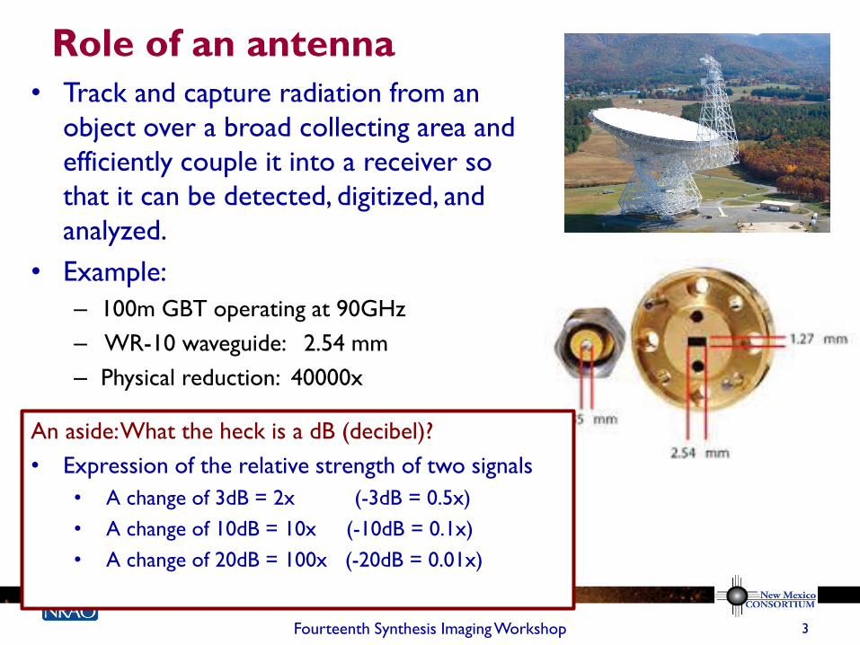
Role of an antenna

• Track and capture radiation from an

object over a broad collecting area and

efficiently couple it into a receiver so

that it can be detected, digitized, and

analyzed.

• Example:

– 100m GBT operating at 90GHz

– WR-10 waveguide: 2.54 mm

– Physical reduction: 40000x


An aside: What the heck is a dB (decibel)?

• Expression of the relative strength of two signals

• A change of 3dB = 2x (-3dB = 0.5x)



Importance of Antenna properties on

your data

Fourteenth Synthesis Imaging Workshop 4

• Antenna amplitude and phase patterns cause amplitude and phase to vary across the field of view.

• Polarization properties of the antenna modify the apparent polarization of the source.

• Antenna pointing errors cause time varying amplitude and phase errors.

• Variation in noise pickup from the ground can cause time-variable amplitude errors.

• Deformations of the antenna surface can cause amplitude and phase errors, especially at short wavelengths.

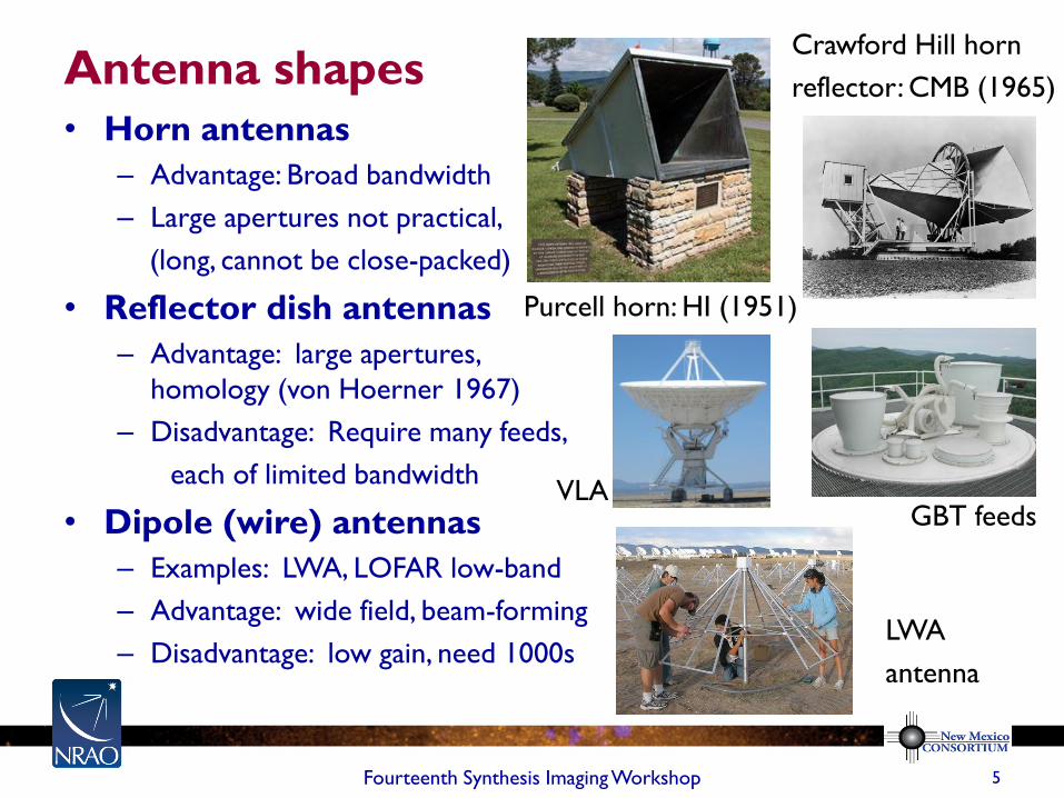
Antenna shapes

• Horn antennas

– Advantage: Broad bandwidth

– Large apertures not practical,

(long, cannot be close-packed)

• Reflector dish antennas

– Advantage: large apertures,

homology (von Hoerner 1967)

– Disadvantage: Require many feeds,

each of limited bandwidth

• Dipole (wire) antennas

– Examples: LWA, LOFAR low-band

– Advantage: wide field, beam-forming

– Disadvantage: low gain, need 1000s


Purcell horn: HI (1951)

Crawford Hill horn

reflector: CMB (1965)

GBT feeds

LWA

antenna

VLA

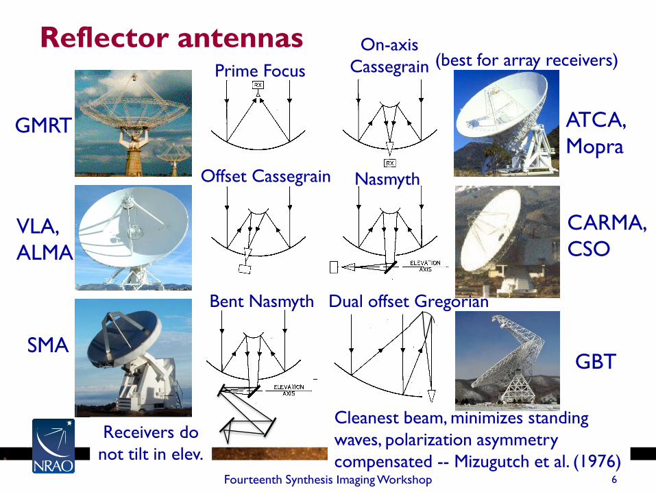
Reflector antennas


Prime Focus

GMRT

GBT

VLA,

ALMA

SMA

ATCA,

Mopra

CARMA,

CSO

Offset Cassegrain

On-axis

Cassegrain

Dual offset Gregorian Bent Nasmyth

Nasmyth

Cleanest beam, minimizes standing

waves, polarization asymmetry

compensated -- Mizugutch et al. (1976)

Receivers do

not tilt in elev.

(best for array receivers)

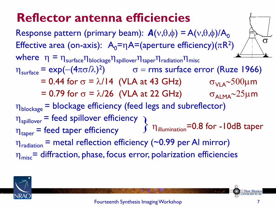
Reflector antenna efficiencies Response pattern (primary beam): A(n,q,f) = A(n,q,f)/A0

Effective area (on-axis): A0=hA=(aperture efficiency)(pR2)

where h = hsurfacehblockagehspilloverhtaperhradiationhmisc

hsurface = exp(-(4ps/l)2) s = rms surface error (Ruze 1966)

= 0.44 for s = l/14 (VLA at 43 GHz) sVLA~500mm

= 0.79 for s = l/26 (VLA at 22 GHz) sALMA~25mm

hblockage = blockage efficiency (feed legs and subreflector)

hspillover = feed spillover efficiency

htaper = feed taper efficiency

hradiation = metal reflection efficiency (~0.99 per Al mirror)

hmisc= diffraction, phase, focus error, polarization efficiencies


s

} hillumination=0.8 for -10dB taper

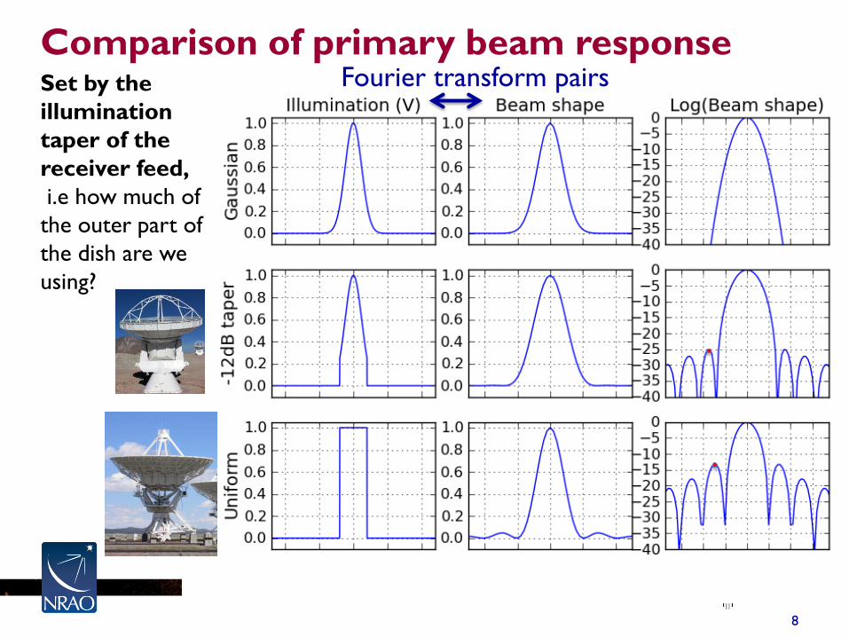
Comparison of primary beam response

q in radians,

l and D in the same units

8

Set by the

illumination

taper of the

receiver feed,

i.e how much of

the outer part of

the dish are we

using?

Fourier transform pairs

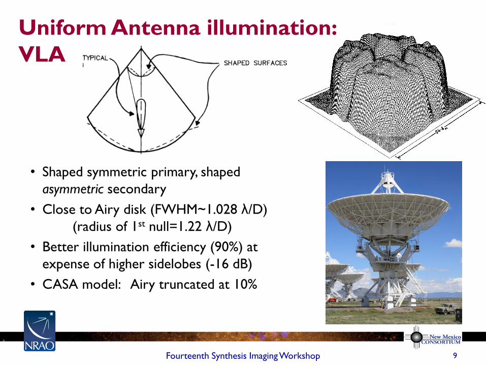
Uniform Antenna illumination:

VLA


• Shaped symmetric primary, shaped

asymmetric secondary

• Close to Airy disk (FWHM~1.028 λ/D)

(radius of 1st null=1.22 λ/D)

• Better illumination efficiency (90%) at

expense of higher sidelobes (-16 dB)

• CASA model: Airy truncated at 10%

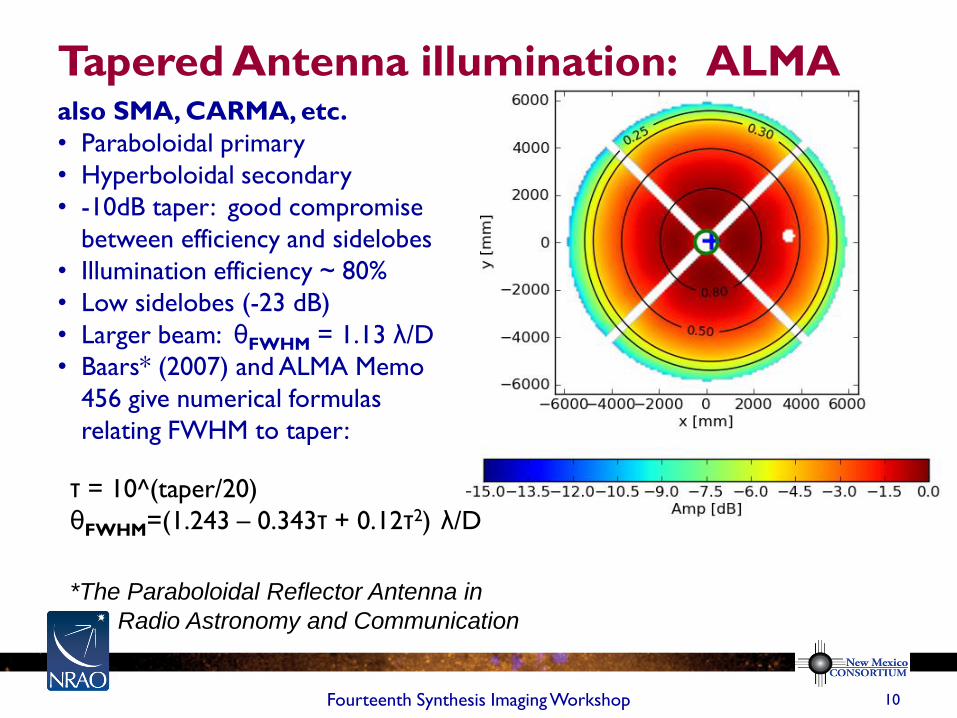
Tapered Antenna illumination: ALMA


also SMA, CARMA, etc.

• Paraboloidal primary

• Hyperboloidal secondary

• -10dB taper: good compromise

between efficiency and sidelobes

• Illumination efficiency ~ 80%

• Low sidelobes (-23 dB)

• Larger beam: θFWHM = 1.13 λ/D

• Baars* (2007) and ALMA Memo

456 give numerical formulas

relating FWHM to taper:

τ = 10^(taper/20)

θFWHM=(1.243 – 0.343τ + 0.12τ2) λ/D

*The Paraboloidal Reflector Antenna in

Radio Astronomy and Communication

Holography is a vital tool The technique of imaging the (complex) beam pattern of an antenna and

Fourier transforming back to the antenna surface illumination (aperture plane)

is known as “holography”. (Napier & Bates 1971, Bennett et al. 1976).

1. Interferometric holography is done with a beacon transmitter on a tower,

or on a satellite, but can also be done on bright quasars, which is called

“astroholography” or “celestial holography”.

2. Non-interferometric holography, also called “out-of-focus (OOF)” or

“phase retrieval”, is useful for measuring large-scale surface error

Holography allows us to measure:

1. Antenna panel misalignment (e.g. ALMA: Baars et al. 2007, IEEE A&PM)

2. Systematic antenna panel mold error (GBT: Hunter et al. 2011, PASP)

3. Large-scale error due to thermal effects (GBT: Nikolic et al. 2007, A&A)

4. Illumination pattern alignment errors (see ALMA Memo 402)

5. Effect of feed legs on the beam


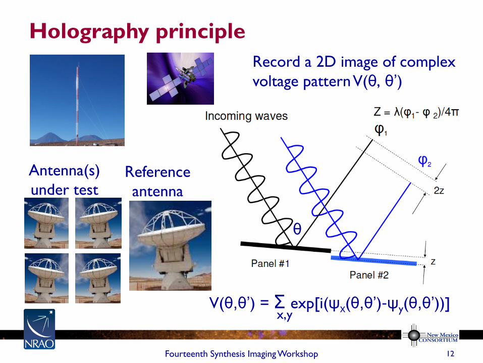
Holography principle


Reference

antenna

Antenna(s)

under test

θ

Record a 2D image of complex

voltage pattern V(θ, θ’)

V(θ,θ’) = Σ exp[i(ψx(θ,θ’)-ψy(θ,θ’))] x,y

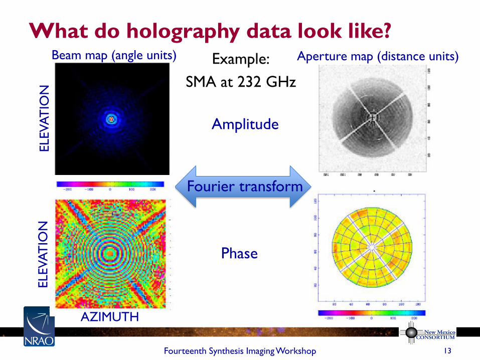
What do holography data look like?


Example:

SMA at 232 GHz

Amplitude

Phase

Beam map (angle units) Aperture map (distance units)

Fourier transform

ELEVA

TIO

N

ELEVA

TIO

N

AZIMUTH

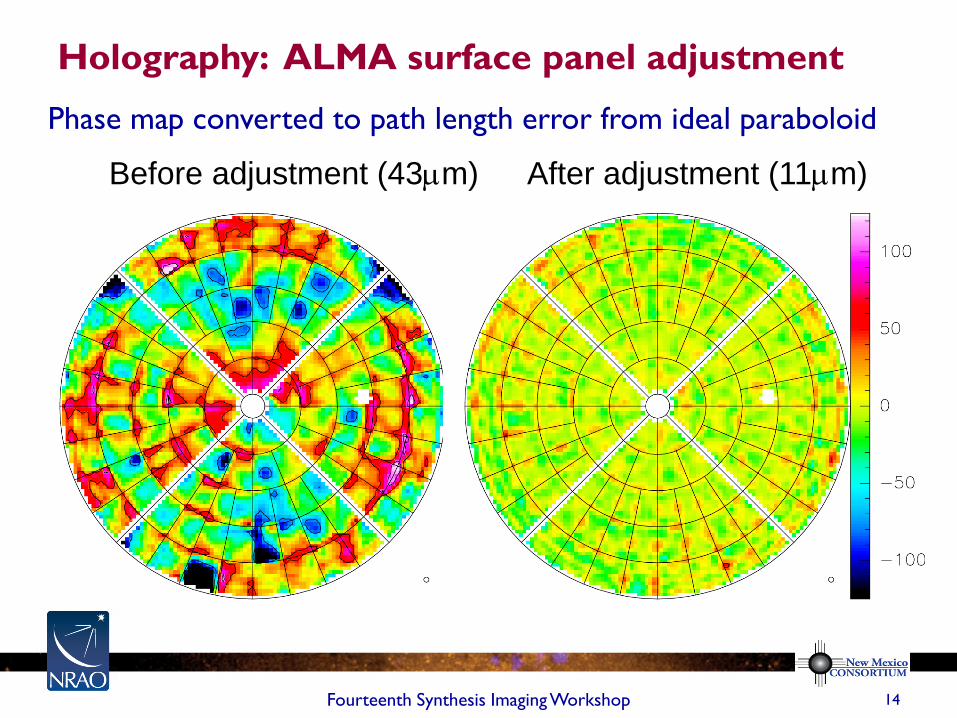
Holography: ALMA surface panel adjustment


Before adjustment (43mm) After adjustment (11mm)

Phase map converted to path length error from ideal paraboloid

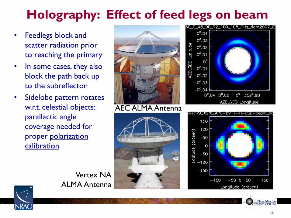
Holography: Effect of feed legs on beam

q in radians,


15

Vertex NA

ALMA Antenna

AEC ALMA Antenna

• Feedlegs block and

scatter radiation prior

to reaching the primary

• In some cases, they also

block the path back up

to the subreflector

• Sidelobe pattern rotates

w.r.t. celestial objects:

parallactic angle

coverage needed for

proper polarization

calibration

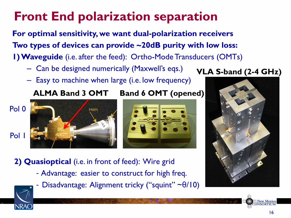
Front End polarization separation

q in radians,


For optimal sensitivity, we want dual-polarization receivers

Two types of devices can provide ~20dB purity with low loss:

1) Waveguide (i.e. after the feed): Ortho-Mode Transducers (OMTs)

– Can be designed numerically (Maxwell’s eqs.)

– Easy to machine when large (i.e. low frequency)

2) Quasioptical (i.e. in front of feed): Wire grid

- Advantage: easier to construct for high freq.

- Disadvantage: Alignment tricky (“squint” ~θ/10)

16

VLA S-band (2-4 GHz)

ALMA Band 3 OMT Band 6 OMT (opened)

Pol 1

Pol 0

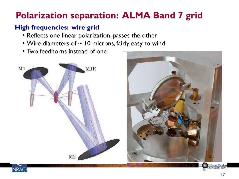
Polarization separation: ALMA Band 7 grid

q in radians,


LO

IF

17

High frequencies: wire grid

• Reflects one linear polarization, passes the other

• Wire diameters of ~ 10 microns, fairly easy to wind

• Two feedhorns instead of one

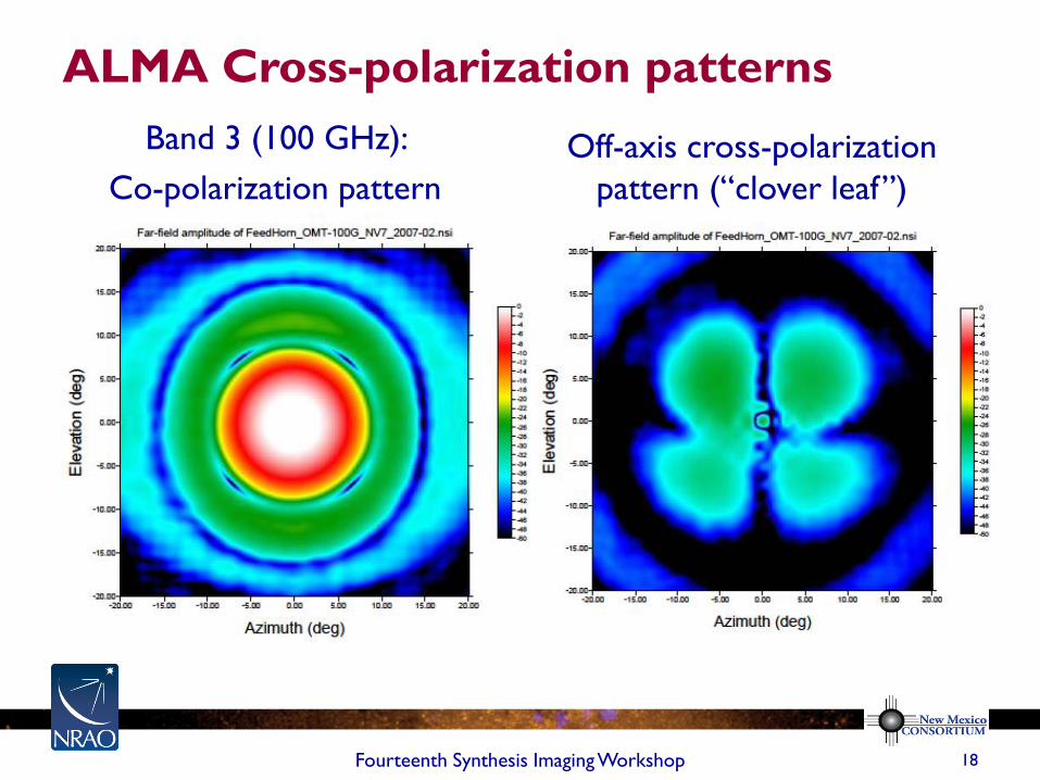
ALMA Cross-polarization patterns


Band 3 (100 GHz):

Co-polarization pattern

Off-axis cross-polarization

pattern (“clover leaf”)

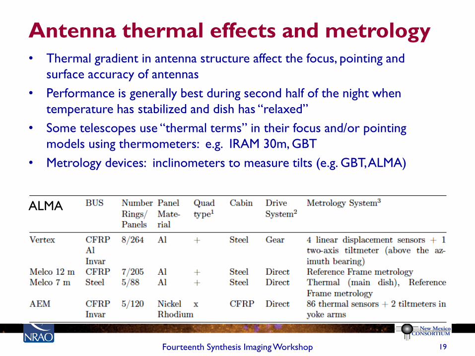
Antenna thermal effects and metrology • Thermal gradient in antenna structure affect the focus, pointing and

surface accuracy of antennas

• Performance is generally best during second half of the night when

temperature has stabilized and dish has “relaxed”

• Some telescopes use “thermal terms” in their focus and/or pointing

models using thermometers: e.g. IRAM 30m, GBT

• Metrology devices: inclinometers to measure tilts (e.g. GBT, ALMA)


ALMA

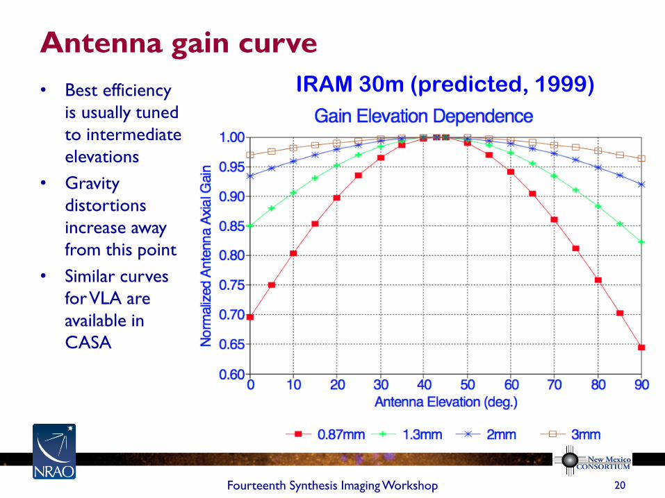
Antenna gain curve


• Best efficiency

is usually tuned

to intermediate

elevations

• Gravity

distortions

increase away

from this point

• Similar curves

for VLA are

available in

CASA

IRAM 30m (predicted, 1999)

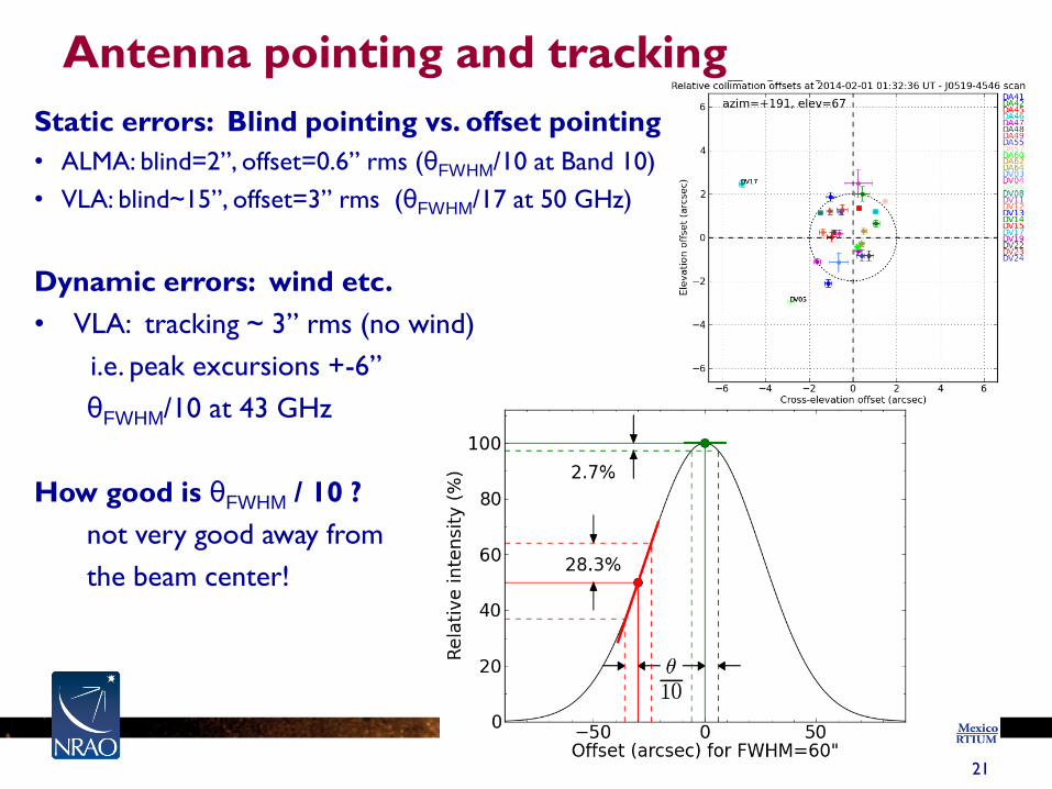
Antenna pointing and tracking

q in radians,


Static errors: Blind pointing vs. offset pointing

• ALMA: blind=2”, offset=0.6” rms (θFWHM/10 at Band 10)

• VLA: blind~15”, offset=3” rms (θFWHM/17 at 50 GHz)

Dynamic errors: wind etc.

• VLA: tracking ~ 3” rms (no wind)

i.e. peak excursions +-6”

θFWHM/10 at 43 GHz

How good is θFWHM / 10 ?

not very good away from

the beam center!

21

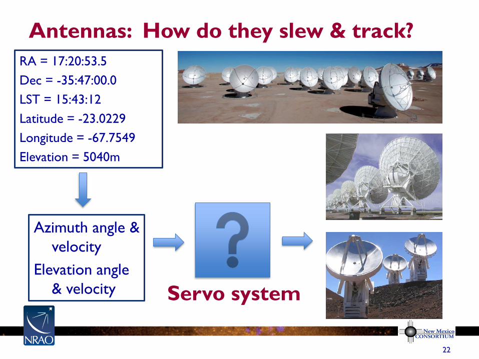
Antennas: How do they slew & track?

RA = 17:20:53.5

Dec = -35:47:00.0

LST = 15:43:12

Latitude = -23.0229

Longitude = -67.7549

Elevation = 5040m

Azimuth angle &

velocity

Elevation angle

& velocity Servo system

22

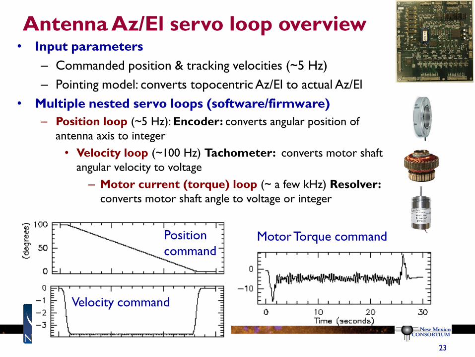
Antenna Az/El servo loop overview

q in radians,


• Input parameters

– Commanded position & tracking velocities (~5 Hz)

– Pointing model: converts topocentric Az/El to actual Az/El

• Multiple nested servo loops (software/firmware)

– Position loop (~5 Hz): Encoder: converts angular position of

antenna axis to integer

• Velocity loop (~100 Hz) Tachometer: converts motor shaft

angular velocity to voltage

– Motor current (torque) loop (~ a few kHz) Resolver:

converts motor shaft angle to voltage or integer

23

Position

command Motor Torque command

Velocity command

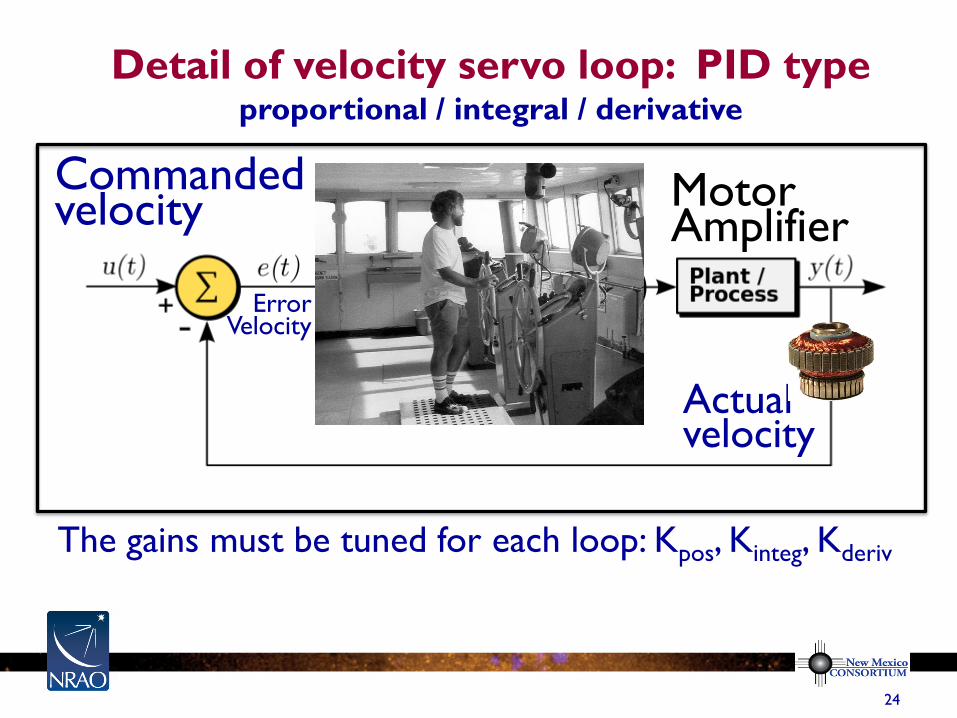
Detail of velocity servo loop: PID type proportional / integral / derivative

Commanded velocity

Actual velocity

Error Velocity

Motor Amplifier

The gains must be tuned for each loop: Kpos, Kinteg, Kderiv

24

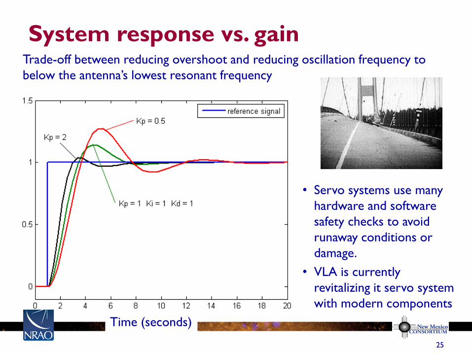
System response vs. gain

25

Trade-off between reducing overshoot and reducing oscillation frequency to

below the antenna’s lowest resonant frequency

• Servo systems use many

hardware and software

safety checks to avoid

runaway conditions or

damage.

• VLA is currently

revitalizing it servo system

with modern components

Time (seconds)

Role of an receiver

Linearly amplify weak RF signals while adding minimal

noise, and downconvert them to room-temperature

output signals at a few GHz (called “IFs”) on coax

cables suitable for digitization

• Receivers are often called “Front Ends” or FE


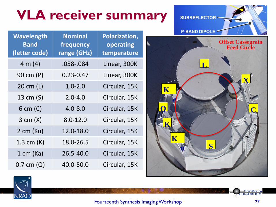
VLA receiver summary


Q Ka K

K

u X

C

S

L

Letter designations

have historical context and are second nature to microwave

engineers.

S

L

C

X

K

a

Q

K

K

u

Offset Cassegrain Feed Circle

Wavelength Band

(letter code)

Nominal frequency

range (GHz)

Polarization, operating

temperature

4 m (4) .058-.084 Linear, 300K

90 cm (P) 0.23-0.47 Linear, 300K

20 cm (L) 1.0-2.0 Circular, 15K

13 cm (S) 2.0-4.0 Circular, 15K

6 cm (C) 4.0-8.0 Circular, 15K

3 cm (X) 8.0-12.0 Circular, 15K

2 cm (Ku) 12.0-18.0 Circular, 15K

1.3 cm (K) 18.0-26.5 Circular, 15K

1 cm (Ka) 26.5-40.0 Circular, 15K

0.7 cm (Q) 40.0-50.0 Circular, 15K

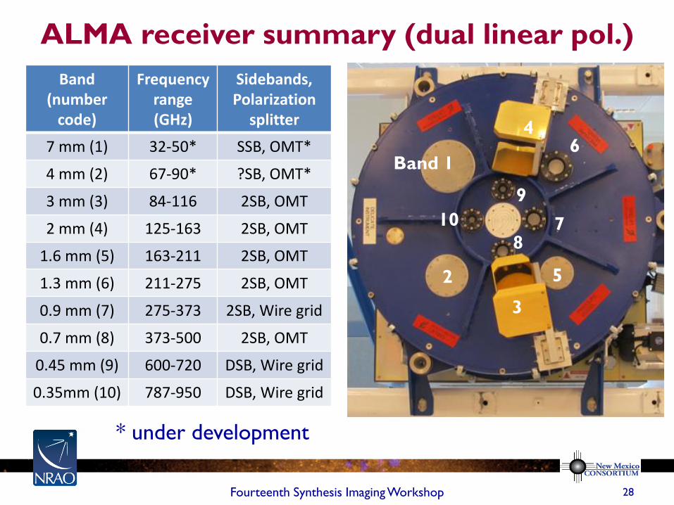
ALMA receiver summary (dual linear pol.)


Q Ka K

K

u X

C

S

L

Letter designations

have historical context and are second nature to microwave

engineers.

Band (number

code)

Frequency range (GHz)

Sidebands, Polarization

splitter

7 mm (1) 32-50* SSB, OMT*

4 mm (2) 67-90* ?SB, OMT*

3 mm (3) 84-116 2SB, OMT

2 mm (4) 125-163 2SB, OMT

1.6 mm (5) 163-211 2SB, OMT

1.3 mm (6) 211-275 2SB, OMT

0.9 mm (7) 275-373 2SB, Wire grid

0.7 mm (8) 373-500 2SB, OMT

0.45 mm (9) 600-720 DSB, Wire grid

0.35mm (10) 787-950 DSB, Wire grid

* under development

Band 1

2

3

4

5

7

6

10

9

8

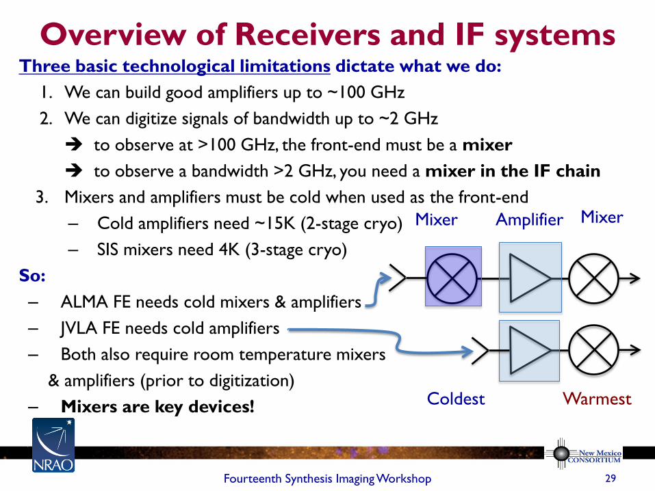
Overview of Receivers and IF systems Three basic technological limitations dictate what we do:

1. We can build good amplifiers up to ~100 GHz

2. We can digitize signals of bandwidth up to ~2 GHz

to observe at >100 GHz, the front-end must be a mixer

to observe a bandwidth >2 GHz, you need a mixer in the IF chain

3. Mixers and amplifiers must be cold when used as the front-end

– Cold amplifiers need ~15K (2-stage cryo)

– SIS mixers need 4K (3-stage cryo)

So:

– ALMA FE needs cold mixers & amplifiers

– JVLA FE needs cold amplifiers

– Both also require room temperature mixers

& amplifiers (prior to digitization)

– Mixers are key devices!


Mixer Amplifier

Coldest Warmest

Mixer

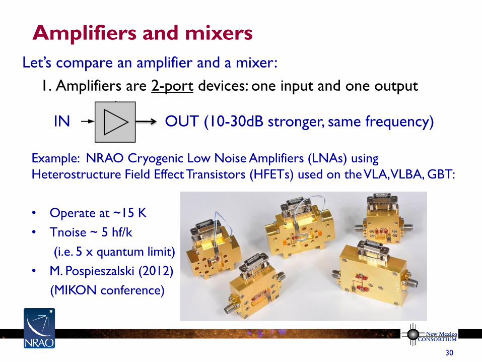
Amplifiers and mixers

Let’s compare an amplifier and a mixer:

1. Amplifiers are 2-port devices: one input and one output

IN OUT (10-30dB stronger, same frequency)

30

q in radians,


Example: NRAO Cryogenic Low Noise Amplifiers (LNAs) using

Heterostructure Field Effect Transistors (HFETs) used on the VLA, VLBA, GBT:

• Operate at ~15 K

• Tnoise ~ 5 hf/k

(i.e. 5 x quantum limit)

• M. Pospieszalski (2012)

(MIKON conference)

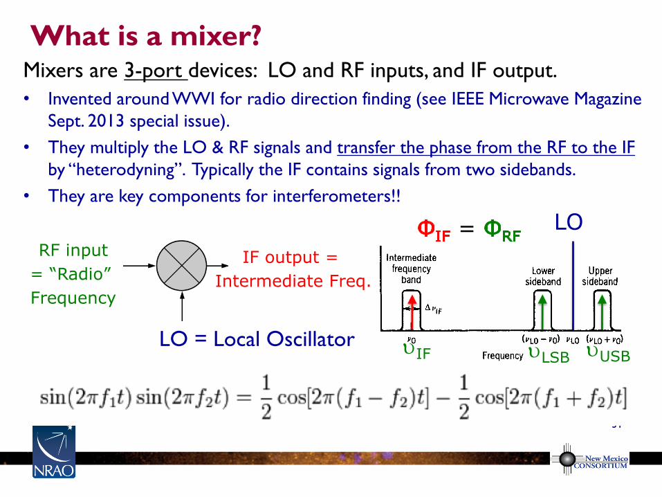
What is a mixer?

31

q in radians,


LO = Local Oscillator

RF input

= “Radio”

Frequency

IF output =

Intermediate Freq.

= LO

uLSB uUSB uIF

Mixers are 3-port devices: LO and RF inputs, and IF output.

• Invented around WWI for radio direction finding (see IEEE Microwave Magazine

Sept. 2013 special issue).

• They multiply the LO & RF signals and transfer the phase from the RF to the IF

by “heterodyning”. Typically the IF contains signals from two sidebands.

• They are key components for interferometers!!

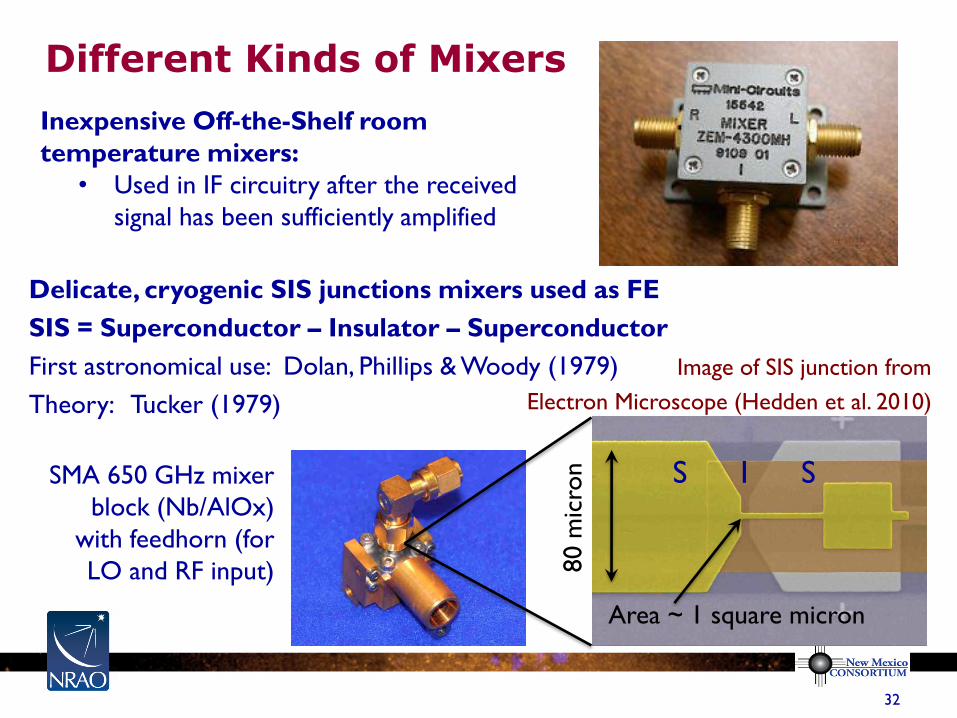
Different Kinds of Mixers

q in radians,


32

Delicate, cryogenic SIS junctions mixers used as FE

SIS = Superconductor – Insulator – Superconductor

First astronomical use: Dolan, Phillips & Woody (1979)

Theory: Tucker (1979)

SMA 650 GHz mixer

block (Nb/AlOx)

with feedhorn (for

LO and RF input)

Image of SIS junction from

Electron Microscope (Hedden et al. 2010)

80 m

icro

n

S I S

Area ~ 1 square micron

Inexpensive Off-the-Shelf room

temperature mixers:

• Used in IF circuitry after the received

signal has been sufficiently amplified

Sidebands

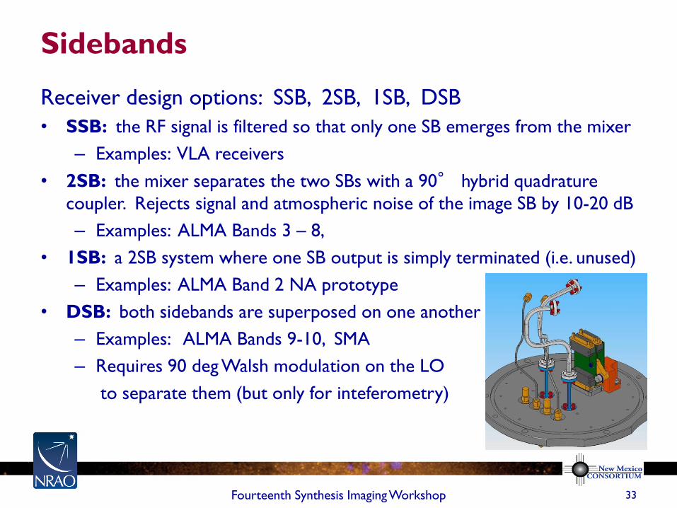
Receiver design options: SSB, 2SB, 1SB, DSB

• SSB: the RF signal is filtered so that only one SB emerges from the mixer

– Examples: VLA receivers

• 2SB: the mixer separates the two SBs with a 90° hybrid quadrature

coupler. Rejects signal and atmospheric noise of the image SB by 10-20 dB

– Examples: ALMA Bands 3 – 8,

• 1SB: a 2SB system where one SB output is simply terminated (i.e. unused)

– Examples: ALMA Band 2 NA prototype

• DSB: both sidebands are superposed on one another

– Examples: ALMA Bands 9-10, SMA

– Requires 90 deg Walsh modulation on the LO

to separate them (but only for inteferometry)


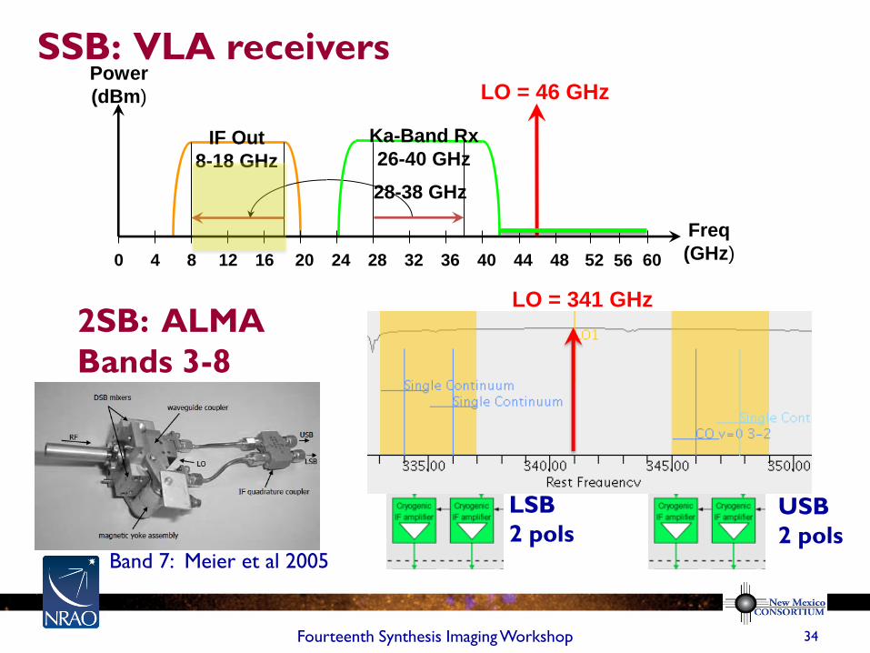
SSB: VLA receivers


Freq

(GHz)

Ka-Band Rx

26-40 GHz IF Out

8-18 GHz

8 12 16 20 24 28 32 36 40 44 48 52 4 0 56 60

LO = 46 GHz

28-38 GHz

Power

(dBm)

2SB: ALMA

Bands 3-8

LSB

2 pols USB

2 pols

LO = 341 GHz

Band 7: Meier et al 2005

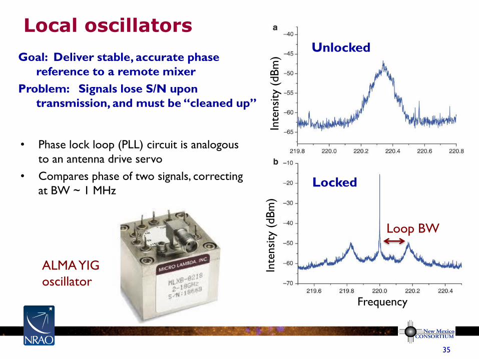
Local oscillators

Goal: Deliver stable, accurate phase

reference to a remote mixer

Problem: Signals lose S/N upon

transmission, and must be “cleaned up”

35

• Phase lock loop (PLL) circuit is analogous

to an antenna drive servo

• Compares phase of two signals, correcting

at BW ~ 1 MHz

Frequency

Inte

nsi

ty (

dB

m)

Inte

nsi

ty (

dB

m)

Unlocked

Locked

ALMA YIG

oscillator

Loop BW

36

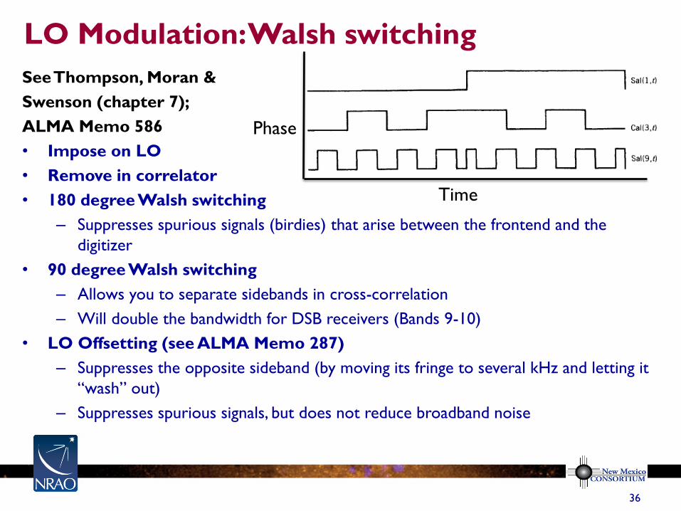
LO Modulation: Walsh switching

See Thompson, Moran &

Swenson (chapter 7);

ALMA Memo 586

• Impose on LO

• Remove in correlator

• 180 degree Walsh switching

– Suppresses spurious signals (birdies) that arise between the frontend and the

digitizer

• 90 degree Walsh switching

– Allows you to separate sidebands in cross-correlation

– Will double the bandwidth for DSB receivers (Bands 9-10)

• LO Offsetting (see ALMA Memo 287)

– Suppresses the opposite sideband (by moving its fringe to several kHz and letting it

“wash” out)

– Suppresses spurious signals, but does not reduce broadband noise

Phase

Time

37

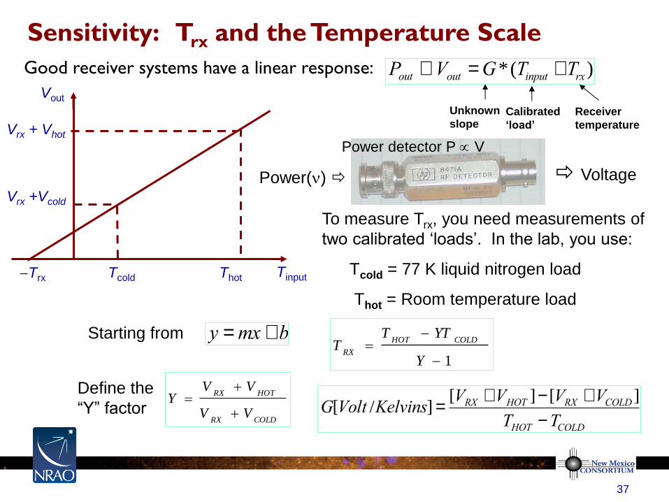
Good receiver systems have a linear response:

Vout

Tinput Tcold Thot

Vrx +Vcold

Vrx + Vhot

-Trx

To measure Trx, you need measurements of

two calibrated ‘loads’. In the lab, you use:

Tcold = 77 K liquid nitrogen load

Thot = Room temperature load

Power(n) Voltage

Power detector P V

Unknown

slope Calibrated

‘load’

Receiver

temperature

Pout µVout =G*(Tinput +Trx)

1-

-=

Y

YTTT

COLDHOT

RX

COLDRX

HOTRX

VV

VVY

=

y =mx + bStarting from

Define the

“Y” factor

G[Volt /Kelvins] =[VRX +VHOT ]- [VRX +VCOLD ]

THOT -TCOLD

Sensitivity: Trx and the Temperature Scale

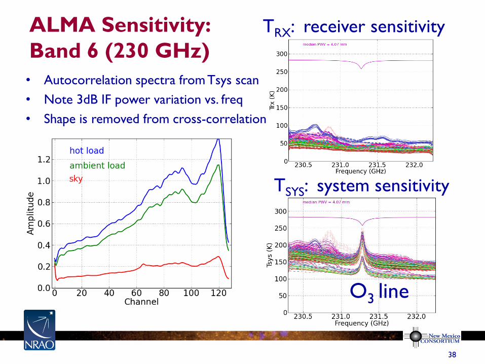
ALMA Sensitivity:

Band 6 (230 GHz)

38

TRX: receiver sensitivity

TSYS: system sensitivity

O3 line

• Autocorrelation spectra from Tsys scan

• Note 3dB IF power variation vs. freq

• Shape is removed from cross-correlation

Thirteenth Synthesis Imaging Workshop - 2012

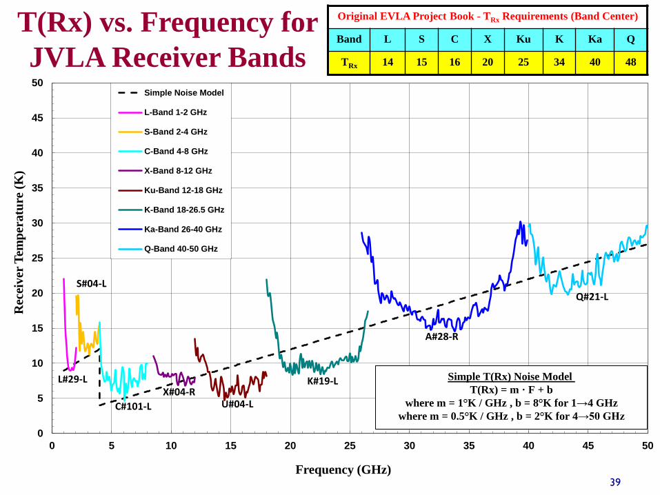
T(Rx) vs. Frequency for

JVLA Receiver Bands

39

0

5

10

15

20

25

30

35

40

45

50

0 5 10 15 20 25 30 35 40 45 50

Rec

eiv

er T

emp

era

ture

(K

)

Frequency (GHz)

Simple Noise Model

L-Band 1-2 GHz

S-Band 2-4 GHz

C-Band 4-8 GHz

X-Band 8-12 GHz

Ku-Band 12-18 GHz

K-Band 18-26.5 GHz

Ka-Band 26-40 GHz

Q-Band 40-50 GHz

L#29-L

C#101-L

X#04-R K#19-L

A#28-R

Q#21-L S#04-L

U#04-L

Simple T(Rx) Noise Model

T(Rx) = m · F + b

where m = 1°K / GHz , b = 8°K for 1→4 GHz

where m = 0.5°K / GHz , b = 2°K for 4→50 GHz

Original EVLA Project Book - TRx Requirements (Band Center)

Band L S C X Ku K Ka Q

TRx 14 15 16 20 25 34 40 48

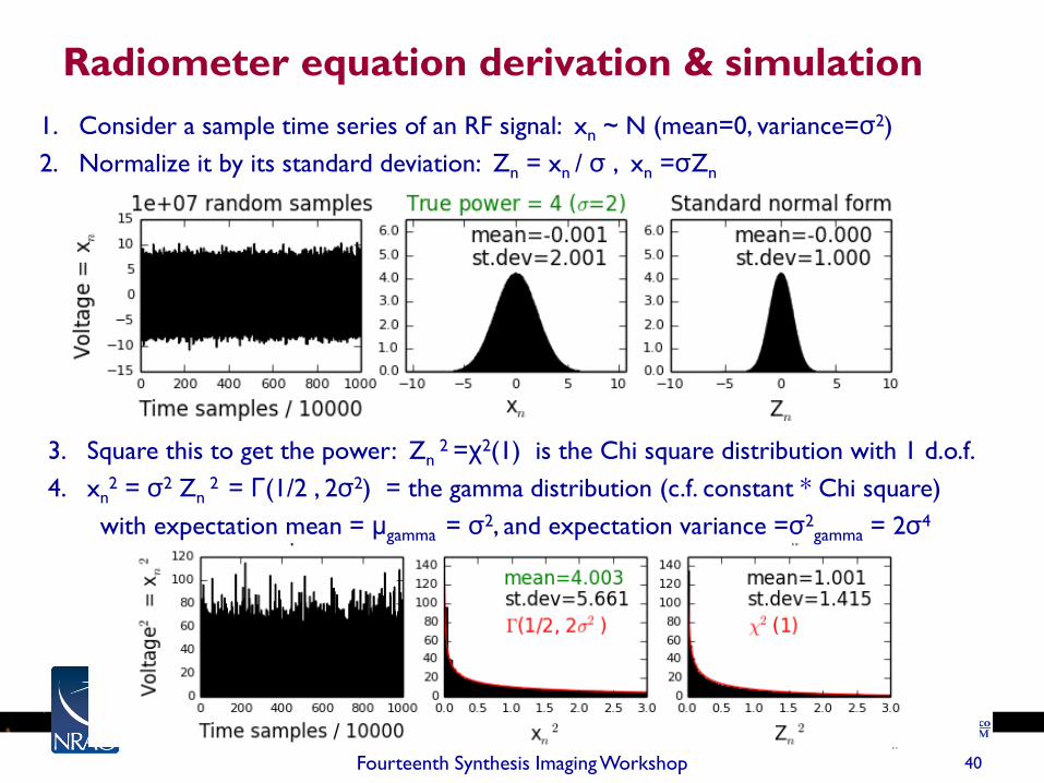
Radiometer equation derivation & simulation

1. Consider a sample time series of an RF signal: xn ~ N (mean=0, variance=σ2)

2. Normalize it by its standard deviation: Zn = xn / σ , xn =σZn


3. Square this to get the power: Zn 2 =χ2(1) is the Chi square distribution with 1 d.o.f.

4. xn2 = σ2 Zn

2 = Γ(1/2 , 2σ2) = the gamma distribution (c.f. constant * Chi square)

with expectation mean = μgamma = σ2, and expectation variance =σ2gamma = 2σ4

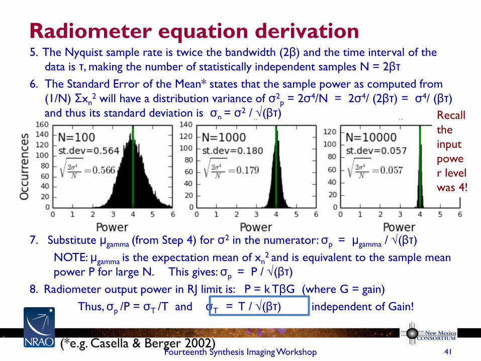
Radiometer equation derivation 5. The Nyquist sample rate is twice the bandwidth (2β) and the time interval of the

data is τ, making the number of statistically independent samples N = 2βτ

6. The Standard Error of the Mean* states that the sample power as computed from

(1/N) Σxn2 will have a distribution variance of σ2

p = 2σ4/N = 2σ4/ (2βτ) = σ4/ (βτ)

and thus its standard deviation is σp = σ2 / √(βτ)

7. Substitute μgamma (from Step 4) for σ2 in the numerator: σp = μgamma / √(βτ)

NOTE: μgamma is the expectation mean of xn2 and is equivalent to the sample mean

power P for large N. This gives: σp = P / √(βτ)

8. Radiometer output power in RJ limit is: P = k TβG (where G = gain)

Thus, σp /P = σT /T and σT = T / √(βτ) independent of Gain!

41 Fourteenth Synthesis Imaging Workshop (*e.g. Casella & Berger 2002)

Recall

the

input

powe

r level

was 4!

Conclusions and Further reading

• For more information on ALMA antennas, receivers, and correlators, see

the ALMA Technical Handbook at http://almascience.org

• Also, see my ADS Private Library on ALMA technology:

http://adsabs.harvard.edu/cgi-bin/nph-

abs_connect?library&libname=ALMA+technology&libid=464295c89a

• And my ADS Private Library on holography:

libname=Holography&libid=464295c89a

• For more info on EVLA receivers:

http://www.aoc.nrao.edu/~pharden/fe/fe.htm


• Knowing a bit about the signal path can really help you understand your

data, especially when there are problems or caveats (such as just how

good is that primary beam correction?)

Extra Slides


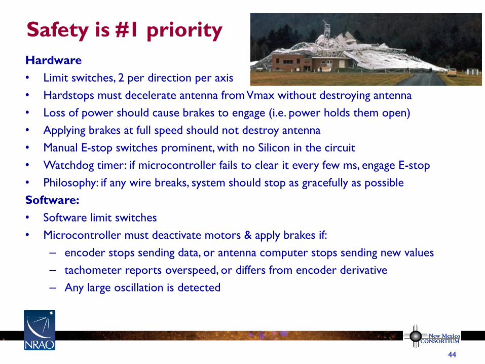
Safety is #1 priority

44

Hardware

• Limit switches, 2 per direction per axis

• Hardstops must decelerate antenna from Vmax without destroying antenna

• Loss of power should cause brakes to engage (i.e. power holds them open)

• Applying brakes at full speed should not destroy antenna

• Manual E-stop switches prominent, with no Silicon in the circuit

• Watchdog timer: if microcontroller fails to clear it every few ms, engage E-stop

• Philosophy: if any wire breaks, system should stop as gracefully as possible

Software:

• Software limit switches

• Microcontroller must deactivate motors & apply brakes if:

– encoder stops sending data, or antenna computer stops sending new values

– tachometer reports overspeed, or differs from encoder derivative

– Any large oscillation is detected

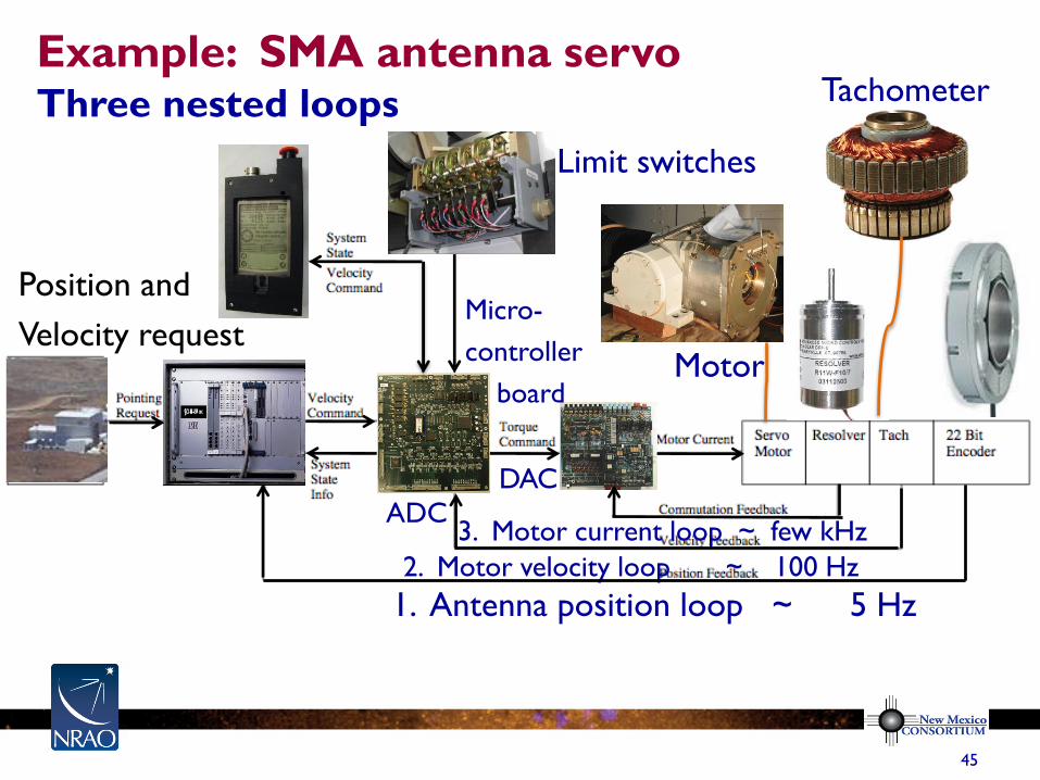
Example: SMA antenna servo Three nested loops

1. Antenna position loop ~ 5 Hz 2. Motor velocity loop ~ 100 Hz

3. Motor current loop ~ few kHz

45

Micro-

controller

board

DAC

ADC

Position and

Velocity request Motor

Limit switches

Tachometer

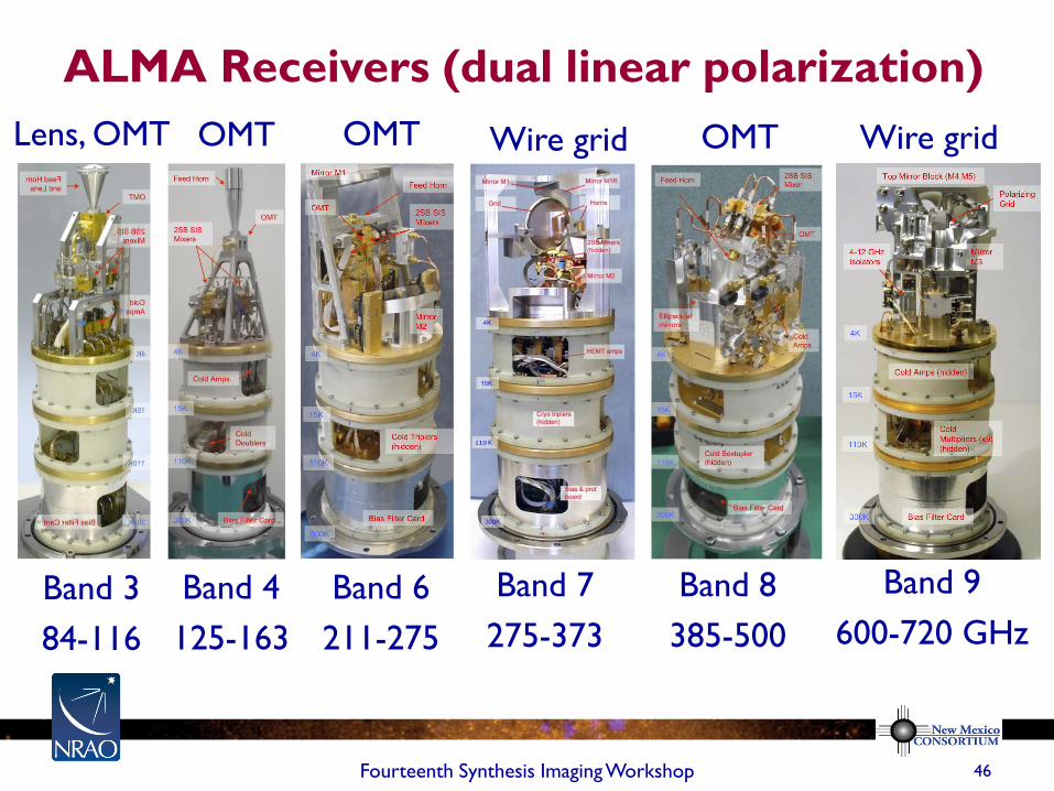
ALMA Receivers (dual linear polarization)


Lens, OMT

Band 4

125-163

Band 6

211-275

Band 7

275-373

Band 8

385-500

Band 9

600-720 GHz

OMT OMT Wire grid OMT Wire grid

Band 3

84-116

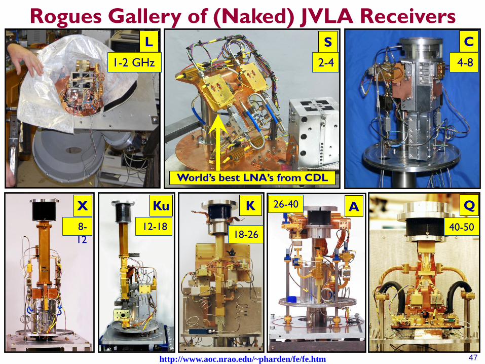
Rogues Gallery of (Naked) JVLA Receivers

Thirteenth Synthesis Imaging Workshop - 2012 http://www.aoc.nrao.edu/~pharden/fe/fe.htm

L S

X Ku K Q

C

47

A

World’s best LNA’s from CDL

1-2 GHz 2-4 4-8

8-

12

12-18 40-50 18-26

26-40

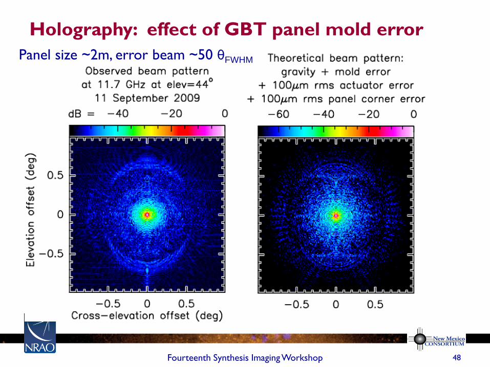
Holography: effect of GBT panel mold error


Panel size ~2m, error beam ~50 θFWHM

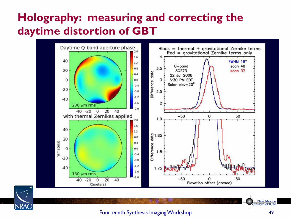
Holography: measuring and correcting the

daytime distortion of GBT


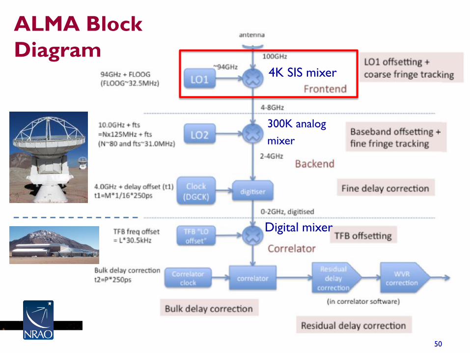
50

ALMA Block

Diagram 4K SIS mixer

300K analog

mixer

Digital mixer

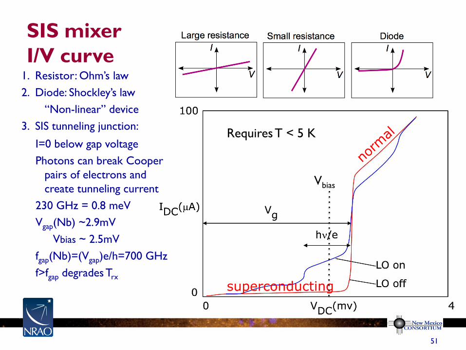
SIS mixer

I/V curve

q in radians,


51

1. Resistor: Ohm’s law

2. Diode: Shockley’s law

“Non-linear” device

3. SIS tunneling junction:

superconducting

I=0 below gap voltage

Photons can break Cooper

pairs of electrons and

create tunneling current

230 GHz = 0.8 meV

Vgap(Nb) ~2.9mV

Vbias ~ 2.5mV

fgap(Nb)=(Vgap)e/h=700 GHz

f>fgap degrades Trx

Requires T < 5 K

Vbias

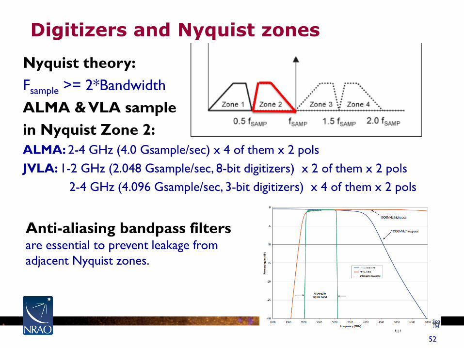
Digitizers and Nyquist zones

q in radians,


Anti-aliasing bandpass filters are essential to prevent leakage from

adjacent Nyquist zones.

52

Nyquist theory:

Fsample >= 2*Bandwidth

ALMA & VLA sample

in Nyquist Zone 2:

ALMA: 2-4 GHz (4.0 Gsample/sec) x 4 of them x 2 pols

JVLA: 1-2 GHz (2.048 Gsample/sec, 8-bit digitizers) x 2 of them x 2 pols

2-4 GHz (4.096 Gsample/sec, 3-bit digitizers) x 4 of them x 2 pols

53

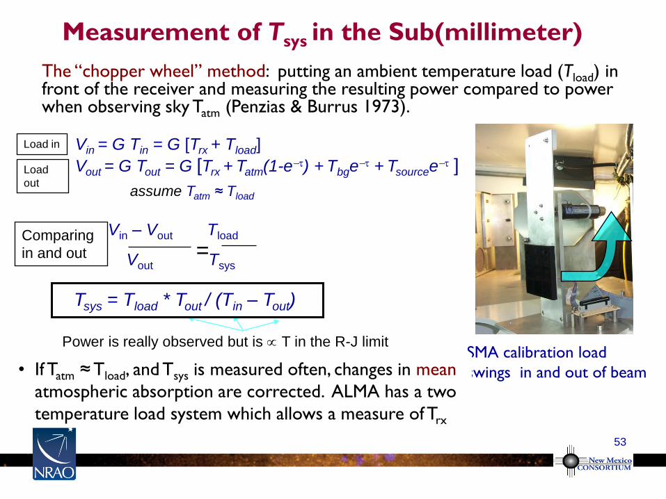
Measurement of Tsys in the Sub(millimeter)

Power is really observed but is T in the R-J limit

Tsys = Tload * Tout / (Tin – Tout)

Vin = G Tin = G [Trx + Tload] Vout = G Tout = G [Trx + Tatm(1-e-t) + Tbge

-t + Tsourcee-t ]

SMA calibration load

swings in and out of beam

Load in

Load

out

• If Tatm ≈ Tload, and Tsys is measured often, changes in mean

atmospheric absorption are corrected. ALMA has a two

temperature load system which allows a measure of Trx

The “chopper wheel” method: putting an ambient temperature load (Tload) in front of the receiver and measuring the resulting power compared to power when observing sky Tatm (Penzias & Burrus 1973).

Vin – Vout Tload

Vout Tsys =

Comparing

in and out

assume Tatm ≈ Tload


ALMA

Documents

Antennas and Receivers - Science Website · PDF fileAntennas and Receivers ... efficiently couple it into a receiver so that it can be detected, ... VLA S-band (2-4 GHz) ALMA Band