ANTENNAS FOR WV BAND APPLICATIONS

University of New MexicoUNM Digital Repository

Electrical and Computer Engineering ETDs Engineering ETDs

Spring 2-19-2018

ANTENNAS FOR WV BAND APPLICATIONSFiras AyoubDoctoral Student, Electrical Engineering

Follow this and additional works at: https://digitalrepository.unm.edu/ece_etds

Part of the Electromagnetics and Photonics Commons

This Dissertation is brought to you for free and open access by the Engineering ETDs at UNM Digital Repository. It has been accepted for inclusion inElectrical and Computer Engineering ETDs by an authorized administrator of UNM Digital Repository. For more information, please [email protected].

Recommended CitationAyoub, Firas. "ANTENNAS FOR WV BAND APPLICATIONS." (2018). https://digitalrepository.unm.edu/ece_etds/408

https://digitalrepository.unm.edu?utm_source=digitalrepository.unm.edu%2Fece_etds%2F408&utm_medium=PDF&utm_campaign=PDFCoverPages

https://digitalrepository.unm.edu/ece_etds?utm_source=digitalrepository.unm.edu%2Fece_etds%2F408&utm_medium=PDF&utm_campaign=PDFCoverPages

https://digitalrepository.unm.edu/eng_etds?utm_source=digitalrepository.unm.edu%2Fece_etds%2F408&utm_medium=PDF&utm_campaign=PDFCoverPages

https://digitalrepository.unm.edu/ece_etds?utm_source=digitalrepository.unm.edu%2Fece_etds%2F408&utm_medium=PDF&utm_campaign=PDFCoverPages

http://network.bepress.com/hgg/discipline/271?utm_source=digitalrepository.unm.edu%2Fece_etds%2F408&utm_medium=PDF&utm_campaign=PDFCoverPages

https://digitalrepository.unm.edu/ece_etds/408?utm_source=digitalrepository.unm.edu%2Fece_etds%2F408&utm_medium=PDF&utm_campaign=PDFCoverPages

mailto:[email protected]

i

Firas Nazem Ayoub Candidate

Electrical and Computer Engineering

Department

This dissertation is approved, and it is acceptable in quality and form for publication:

Approved by the Dissertation Committee:

Christos Christodoulou , Chairperson

Mark Gilmore

Joseph Costantine

Emil Ardelean

ii

ANTENNAS FOR WV BAND APPLICATIONS

by

FIRAS NAZEM AYOUB

Bachelor of Engineering in Computer and Communication

American University of Beirut, 2011

Master of Science in Electrical Engineering

The University of New Mexico, 2013

DISSERTATION

Submitted in Partial Fulfillment of the

Requirements for the Degree of

Doctor of Philosophy

in Engineering

The University of New Mexico

Albuquerque, New Mexico

May, 2018

iii

Dedication

To my dear father, Nazem

My loving mother, Safiya

And my beloved sister, Amal

iv

ACKNOWLEDGEMENT

I sincerely acknowledge my adviser Prof. Christos Christodoulou for all his support,

advisement and mentoring throughout my years of studying. I appreciate all he has done

for me ever since I joined his research group. He is a great mind and it is an honor to be

mentored by him.

I would like to acknowledge Prof. Joseph Costantine for his consistent support over the

years. I am deeply thankful for all his help, insightful comments and motivating feedback

throughout this work.

I would like to acknowledge Prof. Youssef Tawk for his absolute help and support since

I stepped foot in Albuquerque. I thank him for always sharing knowledge with me, being

a great experimental teacher and motivating me throughout the years.

I greatly thank Dr. Emil Ardelean for all his input and help in manufacturing all the

antenna designs presented in this work.

I would like to thank Prof. Mark Gilmore for being on my committee. I appreciate his

great knowledge and modesty.

I would like to thank the Air Force Research Lab for funding this work.

Finally, I would like to acknowledge my family for their unconditional support over

the years. In addition, I would like to thank my friends everywhere for their constant

support.

v

Antennas for WV Band Applications

by

Firas Nazem Ayoub

B.E. in Computer and Communication, The American University of Beirut, 2011

M.S. in Electrical Engineering, University of New Mexico, 2013

Ph.D in Engineering, University of New Mexico, 2018

Abstract

This dissertation focuses on designing, fabricating and testing antennas that are suitable

for operation within the V/W bands. In particular, this work focuses on the design of slotted

rectangular waveguide antenna arrays and cross slotted waveguide fed horn antennas.

These structures are known for their high efficiency and high circularly polarized gain that

can be implemented in satellite and terrestrial communication links. In addition, such

designs can be implemented in radar applications that operate infrequency bands around

72 GHz or 84 GHz bands. Such antenna structures are inexpensive to fabricate since they

can simply be machined using high precision conventional methods (like milling) and laser

cutting when suitable.

In particular, this dissertation discusses two designs involving cross-slotted

waveguides. The first one consists of an array of cross slotted rectangular waveguide

antennas exhibiting radiation beams with Left Hand or Right Hand circular polarization.

The array is composed of 8x16 elements and generates a circularly polarized gain of 25 dB

over the frequency range 84.2 – 85.7 GHz. The array also exhibits a cross polarization

vi

discrimination of more than 20 dB and an isolation of more than 20 dB between the feeding

ports. A new type of z-arm shaped cross slots is introduced that fits on the broad-wall of

a conventional rectangular waveguide. The feeding network is also optimized to regulate

the power and the phase of each rectangular waveguide element in order to increase the

gain of the antenna array.

This dissertation also presents the theoretical analysis of the second design which is a

cross slotted waveguide polarizer. The polarizer achieves a RHCP or LHCP by altering the

feeding ports. The polarizer feeds different conical horns or pyramidal horns without

affecting their characteristics. The efficiency of the polarizer is improved by combining the

power of different crossed slots using square waveguide combiners. Other modes of

operation of the cross slot polarizer are investigated for multiband operation and an antenna

system operating at 72 GHz and 84 GHz simultaneously is designed.

vii

Table of Contents

List of Figures .............................................................................................................. x

List of Tables .......................................................................................................... xviii

....................................................................................... 1

Motivation .................................................................................................... 1

Applications .................................................................................................. 2

WTLE Experiment ....................................................................................... 6

Dissertation Goals ........................................................................................ 8

......................................................................... 10

Slotted Rectangular Waveguides ................................................................ 10

Waveguide Polarizers ................................................................................. 14

Corrugated waveguide polarizers and Iris Polarizers: ................................ 14

Dielectric Septum Loading Polarizer: ......................................................... 17

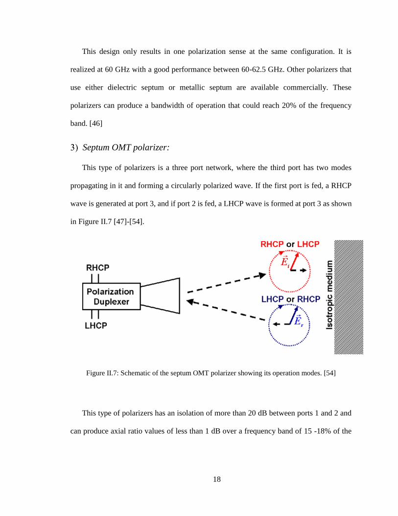
Septum OMT polarizer: .............................................................................. 18

CROSS SLOTTED RECTANGULAR WAVEGUIDE ARRAY .......... 21

Introduction ................................................................................................ 21

Design of Z-Shaped Cross-Slot .................................................................. 22

Design of a Waveguide Array .................................................................... 26

Single Waveguide with Multiple Slots: ...................................................... 26

2-D Waveguide Array with 16 Slots:.......................................................... 29

Feeding Network Design ............................................................................ 32

Full Array Design ....................................................................................... 37

Measured Results ....................................................................................... 40

viii

Conclusion .................................................................................................. 46

CROSS SLOT POLARIZER .................................................................. 48

I. Introduction ................................................................................................ 48

II. Slot Radiating Into a Circular Waveguide ................................................. 49

Theory ......................................................................................................... 49

Design ......................................................................................................... 56

III. A Single Slot Feeding a Conical Horn Antenna ......................................... 62

Horn Antenna Design ................................................................................. 62

Full System Design ..................................................................................... 65

Fabrication Results...................................................................................... 70

IV. Slot Radiating Into a Square Waveguide ................................................... 75

Theory ......................................................................................................... 75

Design ......................................................................................................... 79

V. A Single Slot Feeding a Pyramidal Horn Antenna ..................................... 82

Horn Antenna Design ................................................................................. 82


VI. Dual Slot Polarizer Using Serpentine Power Combiner ............................ 88

Slots Design ................................................................................................ 88

Serpentine Power Combiner Design ........................................................... 90

Full System Design and Performance ......................................................... 91

VII. Dual Slot Polarizer Using A Square Waveguide Power Combiner ........... 95

Dual Slot Design ......................................................................................... 96


ix

Results ......................................................................................................... 99

VIII. Multi-Band Slot Polarizer Design ............................................................ 105

Concept ..................................................................................................... 105

Dual Horn Design ..................................................................................... 106

Single Horn Full System Design............................................................... 110

IX. Conclusion ................................................................................................ 114

.................................................... 115

Appendix A: LIQUID CRYSTAL RECONFIGURABLE ANTENNA DESIGNS

................................................................................................................................... 117

Liquid Crystal Properties at Microwave Frequencies .............................. 117

Frequency Tunable Array Designed at X-band ........................................ 118

Design ....................................................................................................... 118

Simulated Results...................................................................................... 120

Measured Results ...................................................................................... 121

Frequency tunable and Beam Steering Array Design at W/V band. ........ 123

Design ....................................................................................................... 124

Results ....................................................................................................... 126

Fabrication and Measurement: .................................................................. 129

References ................................................................................................................ 132

x

List of Figures

Figure I.1: (a) The traditional two radar systems used for long range and medium range

detection, (b) the combined radar system used for both detection types.[10] .................... 3

Figure I.2: Imaging used to detect concealed weapons. [13] .............................................. 4

Figure I.3: High data rate indoor wireless communication system. [16] ............................ 5

Figure I.4 The transmitter on top of Sandia Peak (left); the V and W-band receivers in

COSMIAC Albuquerque, NM (right); and an illustration of the elevation profile of the

slant path covered by the link (bottom) [23]. ...................................................................... 8

Figure II.1: (a) The configuration of the dipole layer on top of the slot, (b) fabricated

prototype of the parasitic dipoles on top of a slotted waveguide array.[29] ..................... 12

Figure II.2 : Tilted alternating slots with a ridge waveguide. [33] ................................... 12

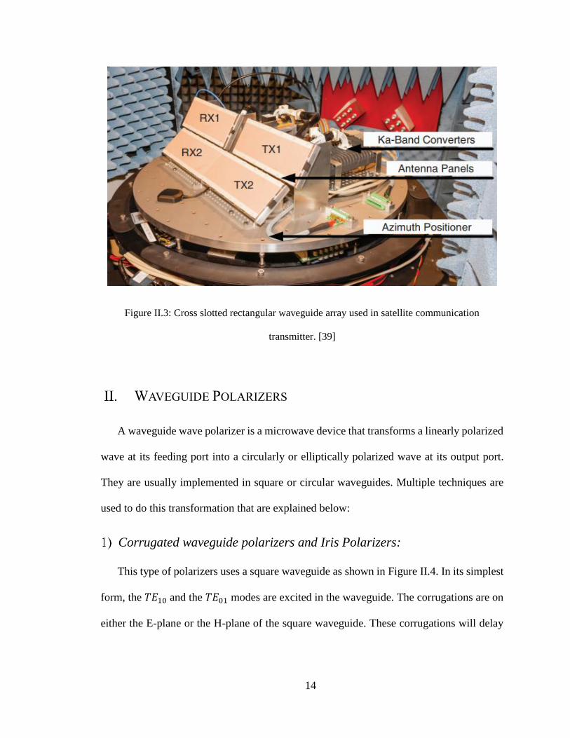
Figure II.3: Cross slotted rectangular waveguide array used in satellite communication

transmitter. [39]................................................................................................................. 14

Figure II.4: (a) Corrugations on the wall of a square waveguide, (b) cross section view of

the waveguide. [40] ........................................................................................................... 15

Figure II.5: Schematic of the irises inside a circular waveguide and the resulting circularly

polarized wave. [44].......................................................................................................... 16

Figure II.6: Schematic of the polarizer using dielectric septum, (a) 3D, (b) cross section

view. [45] .......................................................................................................................... 17

Figure II.7: Schematic of the septum OMT polarizer showing its operation modes. [54] 18

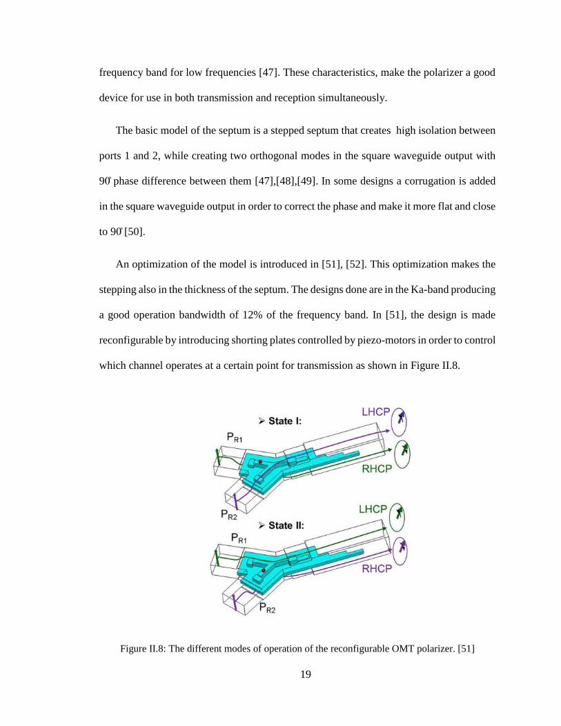
Figure II.8: The different modes of operation of the reconfigurable OMT polarizer. [51]

........................................................................................................................................... 19

xi

Figure III.1: (a) Conventional cross-slot dimensions, (b) The difference between the arm

projection Ap and the slot position s over frequencies, (c) The z-shaped arm cross-slot

structure............................................................................................................................. 24

Figure III.2: The co- and cross-polarization radiation patterns for the conventional and z-

arm slots in the XZ plane. ................................................................................................. 25

Figure III.3: (a) A single WR-10 waveguide element with 4 and 16 slots, (b) The gain

variation as a function of the number of slots. .................................................................. 25

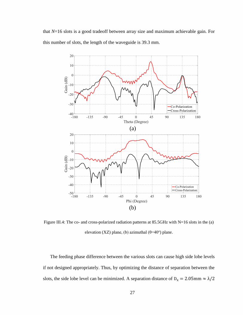
Figure III.4: The co- and cross-polarized radiation patterns at 85.5GHz with N=16 slots in

the (a) elevation (XZ) plane, (b) azimuthal (θ=40o) plane. ............................................... 27

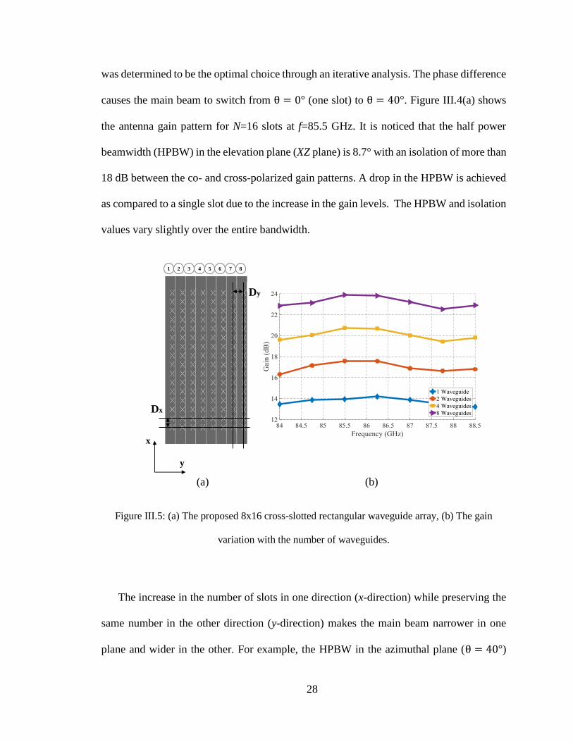
Figure III.5: (a) The proposed 8x16 cross-slotted rectangular waveguide array, (b) The gain

variation with the number of waveguides. ........................................................................ 28

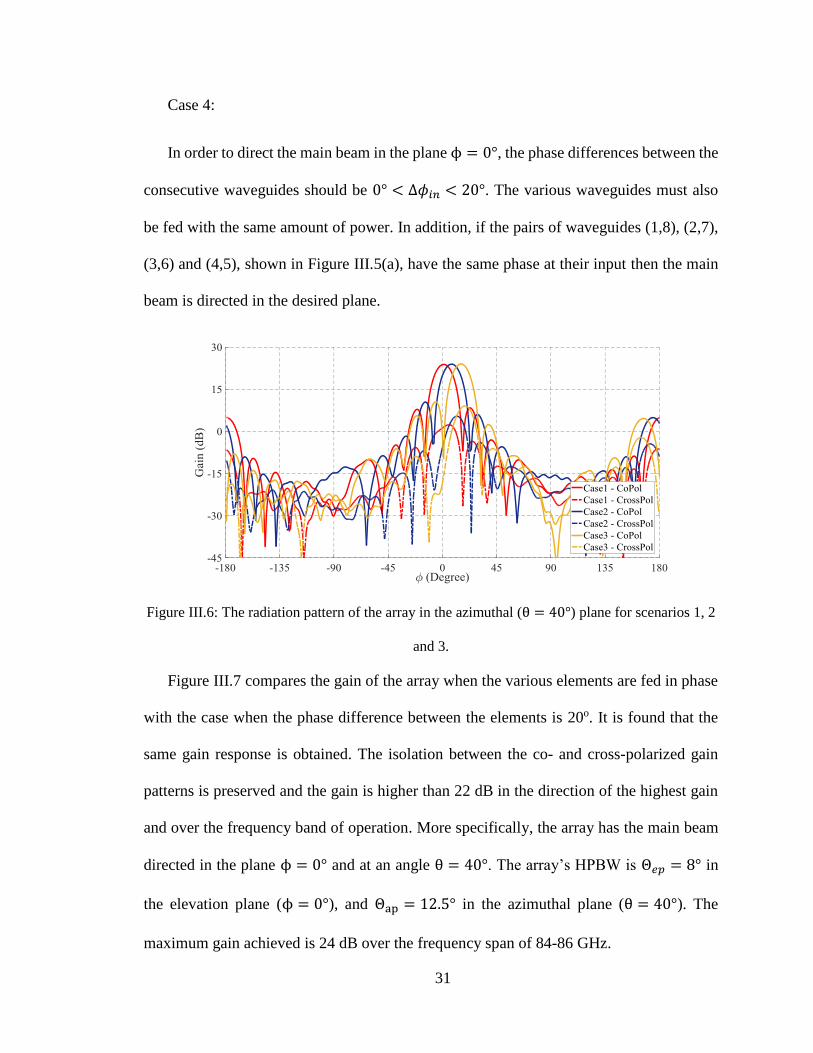
Figure III.6: The radiation pattern of the array in the azimuthal (θ = 40°) plane for

scenarios 1, 2 and 3. .......................................................................................................... 31

Figure III.7: The gain patterns of the array in the azimuthal (θ = 40°) plane for the case

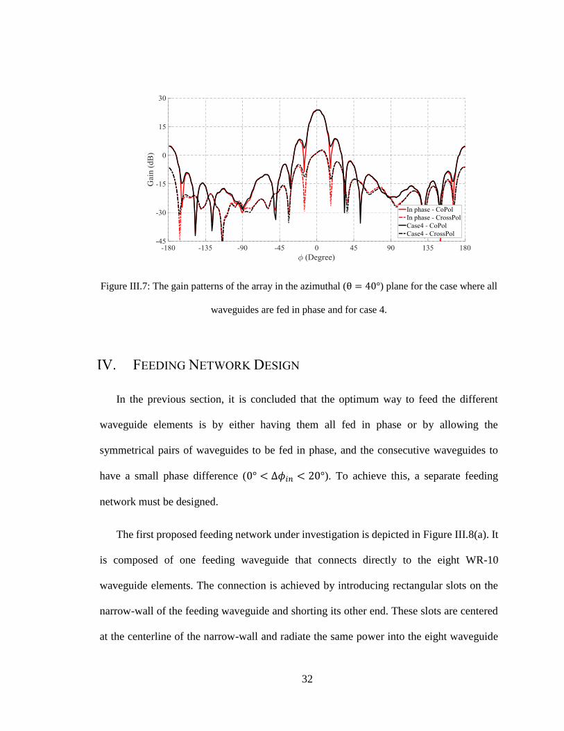
where all waveguides are fed in phase and for case 4. ..................................................... 32

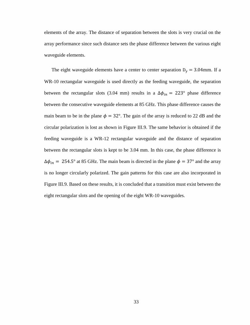
Figure III.8: The proposed feeding with (a) direct connection between the feeding

waveguide and the eight elements WR-10 waveguides, (b) The proposed transition to

achieve the required phase difference between the various elements. .............................. 34

Figure III.9: The gain pattern of the array fed directly by a WR-10 or WR-12 rectangular

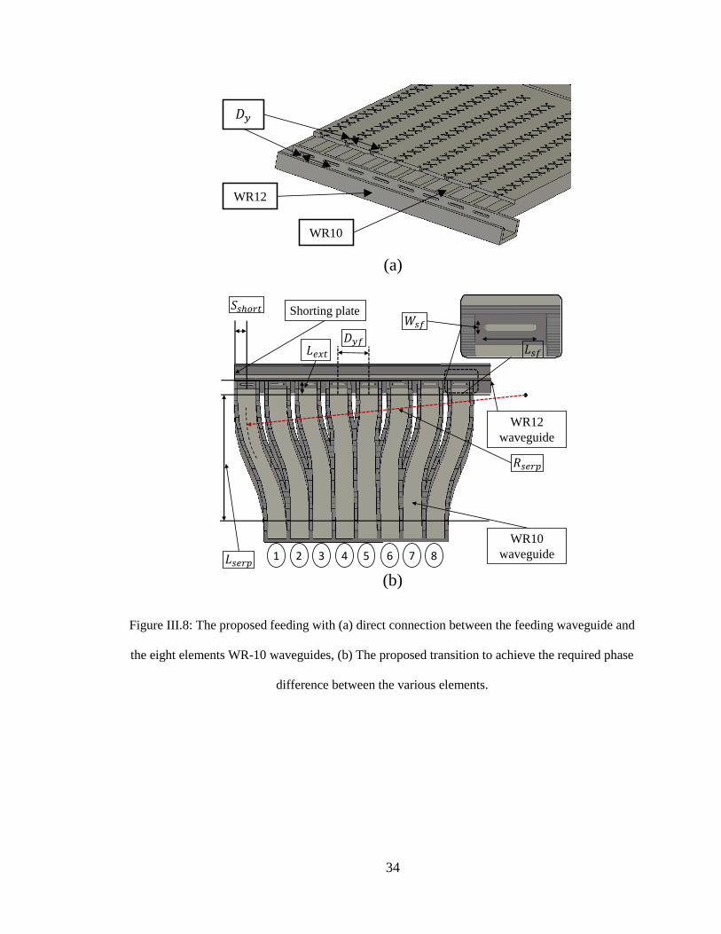
waveguide in the azimuthal (θ = 40o) plane. ..................................................................... 35

Figure III.10: The feeding network S-parameters magnitude in dB and phase in degrees.

........................................................................................................................................... 36

xii

Figure III.11: The full array design (a) disassembled, (b) assembled and (c) radiation

pattern for each port. ......................................................................................................... 38

Figure III.12: (a) The fabricated antenna prototype, (b) The radiation pattern measurement

setup in the (b) elevation plane (ϕ = 0° ) and (c) azimuthal (θ = 40° ). ......................... 41

Figure III.13: (top) The simulated and measured results for the reflection coefficient at both

ports, (bottom) The simulated and measured isolation between the two ports. ................ 42

Figure III.14: Simulated and measured gain patterns of the array in the elevation plane

(𝜙 = 0°) at 85 GHz when (a) port 1 is fed, (b) port 2 is fed. ........................................... 44

Figure III.15: Simulated and measured gain patterns of the array in the azimuth plane (𝜃 =

40°) at 85 GHz when (a) port 1 is fed, (b) port 2 is fed. ................................................... 45

Figure III.16: The isolation between the co- and cross-polarization in the direction of the

maximum gain. ................................................................................................................. 46

Figure IV.1: (a) The slot on the broad-wall of a rectangular waveguide, (b) TE10 mode

fields on the broad-wall of a rectangular waveguide, (c) TE11 mode fields in a circular

waveguide. ........................................................................................................................ 50

Figure IV.2: Plot of the transmission between ports 1 and 3 for different circular slots and

a cross slot operating at 72 GHz. ...................................................................................... 58

Figure IV.3: Plot of the S11 and S21 over frequency for the Z-arm shape cross slot extraction.

........................................................................................................................................... 60

Figure IV.4: Plot of the power received at the end of the circular waveguide in the form of

TE11 mode. ........................................................................................................................ 61

Figure IV.5: Plot of the unwrapped phase of the two TE11 modes at the end of the circular

waveguide. ........................................................................................................................ 61

xiii

Figure IV.6: The absolute gain of a conical horn as a function of aperture diameter (dm/ λ)

for a series of axial lengths, L. [60] .................................................................................. 64

Figure IV.7: Conical horn reflection coefficient............................................................... 65

Figure IV.8: Single slot feeding a conical horn antenna. .................................................. 67

Figure IV.9: Reflection coefficient and the isolation between both ports for both 72 and 84

GHz models. ..................................................................................................................... 69

Figure IV.10: (a) The maximum gain of the 72 and 84 GHz designs vs frequency, compared

to the linear gain of the horn, (b) the axial ratio of the 72 and 84 GHz designs vs frequency.

........................................................................................................................................... 70

Figure IV.11: Gain pattern at 73 GHz, (a) in ϕ = 00, (b) in ϕ = 900. ................................. 70

Figure IV.12: Polarizer assembling technique. ................................................................. 71

Figure IV.13: (a) The conical horn attached to the polarizer, (b) The measurement setup

for the s-parameters of the polarizer. ................................................................................ 72

Figure IV.14: Plot of the measured s-parameters of the polarizer. ................................... 73

Figure IV.15: Plots of the power received by port 3 from port 1 for two orthogonal TE11

modes. ............................................................................................................................... 74

Figure IV.16: Plots of the phase difference between the two orthogonal TE11 modes seen

at port 3. ............................................................................................................................ 74

Figure IV.17: (a) Cross slot on the broad-wall of a rectangular waveguide coupling power

into a square waveguide, (b) 𝑇𝐸10 mode fields in a rectangular waveguide, (c) 𝑇𝐸10 and

𝑇𝐸01 modes Electric fields in a square waveguide. ......................................................... 75

Figure IV.18: The plots of the input reflection coefficient and the isolation between ports

1 and 2 for a square waveguide extraction design. ........................................................... 80

xiv

Figure IV.19: Plot of the power received at the end of the square waveguide in the form

of TE01 and TE10 modes. ................................................................................................... 81

Figure IV.20: Plot of the phase difference between the TE01 and TE10 modes at the end of

the square waveguide. ....................................................................................................... 81

Figure IV.21: Illustration of a pyramidal horn structure. [62] .......................................... 83

Figure IV.22: Layout of the pyramidal horn fed by a cross slot polarizer........................ 84

Figure IV.23: The plots of the input reflection coefficient and the isolation between ports

1 and 2 for a cross slot feeding a pyramidal horn. ............................................................ 84

Figure IV.24: Plot of the Gain over frequency for the 17 dB and 23 dB designs. ............ 86

Figure IV.25: Gain pattern in the planes 𝜙 = 0° and 𝜙 = 90° for both RHCP and LHCP

patterns at 72 GHz. ........................................................................................................... 86

Figure IV.26: Plot of the axial ratio for the 17 dB and 23 dB designs. ............................ 87

Figure IV.27: Cross polarization discrimination plot over frequency. ............................. 87

Figure IV.28: (a) Illustration of the serpentine combiner geometry, (b) Illustration of the

different parts of the system combined. ............................................................................ 91

Figure IV.29: The E-field inside the different parts of the system at 84 GHz. ................. 92

Figure IV.30: The s-parameters of the system with a serpentine power combiner. ......... 92

Figure IV.31: (a) Plot of the comparison of the maximum gain performance; (b) plot of the

comparison between the axial ratios of the serpentine vs the single slot polarizer. ......... 93

Figure IV.32: The LHCP and RHCP radiation pattern of the serpentine fed horn in different

plane cuts at 84 GHz. ........................................................................................................ 95

xv

Figure IV.33: (a) The layout and the different parameters of the square waveguide

combiner, (b) The E-field inside the different sections of the full system at 72 GHz when a

pyramidal horn is connected. ............................................................................................ 98

Figure IV.34: S-parameters comparison between a regular combiner and a combiner with

a ridge.............................................................................................................................. 100

Figure IV.35: Illustration of the design with and without a ridge in the rectangular

waveguide. ...................................................................................................................... 100

Figure IV.36: (a) Gain vs frequency for different designs, (b) Axial ratio vs frequency for

the rectangular waveguide with and without ridge. ........................................................ 102

Figure IV.37: Gain pattern of scenarios 1 and 2 for both LHCP and RHCP when port 1 is

fed at 72.5 GHz. .............................................................................................................. 103

Figure IV.38: S-parameters of the different scenarios vs frequency. ............................. 103

Figure IV.39:(a) Gain comparison vs frequency, (b) Axial ratio comparison vs frequency

for scenarios 1 and 2. ...................................................................................................... 105

Figure IV.40: The full system with two horns. ............................................................... 107

Figure IV.41: S-parameters of the system with two horns operating at 72 and 84 GHz. 108

Figure IV.42: Gain comparison between linear gain of the horn and the system with two

horns. ............................................................................................................................... 109

Figure IV.43: The co-polarization and cross-polarization radiation patterns of the system

at 85 GHz in different plane cuts. ................................................................................... 109

Figure IV.44: The axial ratio of the system with two horns. .......................................... 110

Figure IV.45: The E-field in the system with two square waveguide channels for the

different frequencies of operation. .................................................................................. 111

xvi

Figure IV.46: The single horn full system s-parameters................................................. 112

Figure IV.47: The gain and axial ratio of the system with a single horn. ....................... 112

Figure IV.48: Gain pattern of the single horn system in different plane cuts. ................ 113

Figure A.1: Illustration of liquid crystal transition as a bias voltage is applied. ............ 117

Figure A.2: Illustration of the corporate feed and array layout. ..................................... 119

Figure A.3: (a) 4x4 array of rectangular patches on top with the DC feeding network on

the bottom, (b) The DC feeding network. ....................................................................... 119

Figure A.4: Frequency tuning caused by different combinations of patches with DC = 40V.

......................................................................................................................................... 120

Figure A.5: Gain pattern (E-plane) showing a small shift in the direction of the main beams.

......................................................................................................................................... 121

Figure A.6: Different Antenna Fabrication Layers. ........................................................ 122

Figure A.7: Assembled antenna. ..................................................................................... 122

Figure A.8: Antenna Return Loss caused by different applied DC voltages when all

switches are ON. ............................................................................................................. 123

Figure A.9: Different antenna Return Loss plots for different switch connections at 40 V

DC. .................................................................................................................................. 123

Figure A.10: (a) The different layers of the design, (b) the different feeds in the model and

(c) the LC cavities with the DC control. ......................................................................... 125

Figure A.11: 2x8 Reconfigurable array fed using a rectangular waveguide to microstrip

line transition. ................................................................................................................. 125

Figure A.12: The Reflection Coefficient of the array in different configuration scenarios.

......................................................................................................................................... 127

xvii

Figure A.13: The radiation pattern of the CPW fed array showing beam steering at 84.5

GHz in the H-Plane. ........................................................................................................ 127

Figure A.14: The Reflection Coefficient of the array in different configuration scenarios

......................................................................................................................................... 128

Figure A.15: The radiation pattern of the rectangular waveguide fed array showing beam

steering at different frequencies in the H-Plane. ............................................................. 129

Figure A.16: Antenna fabrication: a) Ground plane layer, b) Feeding network layer and LC

cavities, c) Rectangular patches. ..................................................................................... 130

Figure A.17: Assembled array design. ............................................................................ 130

Figure A.18: Fabricated antenna array input reflection coefficient. ............................... 131

xviii

List of Tables

Table III.1: Dimensions of the different parameters of the array. .................................... 39

Table III.2: The array calculated gain for both ports at different frequencies. ................. 43

Table III.3: Comparison between different planar slotted waveguides working at millimeter

wave frequencies. .............................................................................................................. 43

Table IV.1: Dimensions of the Z-shaped arm cross-slot at 72 GHz. ................................ 59

Table IV.2: Design dimensions for the polarizer at 72 GHz and 84 GHz. ....................... 66

Table IV.3: Pyramidal horn dimensions operating at E-band........................................... 83

Table IV.4: Dimensions of the Z-shaped arm cross-slots at 84 GHz used in the serpentine

power combiner. ............................................................................................................... 89

Table IV.5: Dimensions of the Z-shaped arm cross-slots at 72 GHz used in the square

waveguide power combiner. ............................................................................................. 97

Table IV.6: Dimensions of the Z-shaped arm cross-slots at 72 and 84 GHz used in the

multi-band system. .......................................................................................................... 107

1

INTRODUCTION

MOTIVATION

New communication systems that are able to support a large number of users and high

data rates require researchers to investigate the use of millimeter-wave frequency bands for

communication. These frequency bands are either unassigned, or are less crowded than the

lower end of the frequency spectrum. This availability of these frequency bands ensures

high bandwidths, which in turn ensure high data rates in communication links.

For years, the solution for the congestion of the lower end of the frequency spectrum

was the use of techniques, such as cognitive radio, that allow systems to look for frequency

bands that are free and use them for communication [1]. Another solution was the use of

frequencies in the K and Ka-band ranges, which was made possible by the technological

advancement of RF systems [2]. Nowadays, the use of higher frequencies in the W/V bands

is under research and investigation.

In the millimeter-wave frequency bands, the free space propagation losses (FSPL)

under normal weather conditions are significant for long distance communication. This

loss factor is directly proportional to the distance of the link and inversely proportional to

the wavelength. At these ranges, not all frequencies are suitable for long distance point-to-

point communication links due to the atmospheric absorptions that adds to the losses. For

instance, between 55 – 65 GHz there is an oxygen absorption band that causes wave

2

attenuations of 10 dB/Km. At such frequencies, only short distance communication links

are feasible [3].

For longer distance communication links, in the order of kilometers, increasing the

frequency above 65 GHz does not present any challenges in terms of propagation other

than the propagation losses. The 71-76 GHz and 81-86 GHz in the W/V band frequency

ranges constitute a suitable candidate for such communication links. Propagation at these

frequencies is being studied by the W/V band terrestrial link experiment (WTLE) located

in Albuquerque, NM, USA [4]. These new bands are able to provide ultra-wide

communication bandwidth and can be adopted for space, as well as terrestrial

communications [5],[6]. Recently, these frequency bands were assigned by the Federal

Communications Commission (FCC) to satellite communication and other applications

that do not interfere with this type of communication [7]. The wave propagation at these

frequencies creates some problems under severe weather conditions, which could be an

obstacle to satellite or terrestrial communication. This dissertation presents research that

aims to tackle these problems by designing inexpensive antennas and microwave devices

that can be used for communication or radar systems at these high frequencies.

APPLICATIONS

The W/V frequency bands have short wavelengths that make the wave more sensitive

to small objects and more details in objects. This property is very attractive to high

resolution radars. Multiple radar systems are being deployed at these frequencies. A

monopulse radar system at 94 GHz was developed for high resolution tracking in

antimissile systems or in satellite communication tracking [8]. Another radar system

3

targeting the detection of airport runway debris was developed at 94.5 GHz [9]. Other radar

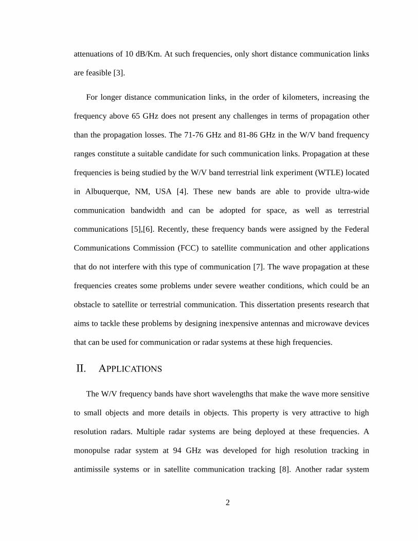
systems at 77 GHz were developed for car collision avoidance systems [10],[11],[12]. This

type of radars can be used for both long range and medium range car detection as shown

in Figure I.1.

Figure I.1: (a) The traditional two radar systems used for long range and medium range detection,

(b) the combined radar system used for both detection types.[10]

Another type of applications developed at W-band frequencies is passive millimeter-

wave imaging [13]. This application takes advantage of the high resolution of the

wavelength, around 3 mm, to detect objects that are unseen in bad visibility conditions.

This technique can be used for both military and civilian purposes, such as detecting

4

concealed weapons, rescue missions under low visibility, low visibility navigation and oil

spill detection. An example of these applications that use imaging is shown in Figure I.2.

Figure I.2: Imaging used to detect concealed weapons. [13]

Finally, due to the availability of large frequency bandwidths at W/V bands, high data

rates communication links are possible. One potential application at 73 GHz is the 5G

cellular network [14],[15]. This application is expected to deliver 6 Gb/s data rates at

multiple frequency bands including a frequency band centered at 73 GHz. This increase in

data rates is necessary due to the increased use of cellular networks and the increased

demand of higher data rates by both the customers and the applications.

Indoor high data rates communication links, reaching Gbps speeds, were also

developed [16],[17],[18]. These applications operate at 60, 87.5 and 94 GHz, producing 3

5

– 25 Gbps data rates. A similar system is shown in Figure I.3. These high data rates ensure

a better quality of service to the customer. These systems especially the one at 60 GHz, are

used in short communication links.

Figure I.3: High data rate indoor wireless communication system. [16]

Since the frequency bands 71-76 GHz and 81-86 GHz are shown to be good candidates

for long distance communications links, satellite communication and earth to satellite

communication is another application at these frequency bands. Recently, the FCC has

declared these frequency bands to be reserved for satellite communications and any other

application that does not interfere with it [7]. Several studies are being conducted to check

the feasibility of such communication systems [19],[20],[21], and a new satellite mission

called WAVE is planned to be deployed in the W-band [20].

For the past two years, the University of New Mexico, in collaboration with the Air

Force research Lab, have been studying the wave propagation at W/V bands under the

WTLE experiment, as a first step in the study of the feasibility of satellite communication

6

at these frequencies. In the next section a more detailed explanation of this experiment is

presented.

WTLE EXPERIMENT

The W/V band Terrestrial Link Experiment (WTLE), is a combined research effort

between the University of New Mexico, the Air Force Research Labs and NASA, aiming

to study the wave propagation at 71-76 GHz and 81 – 86 GHz [22].

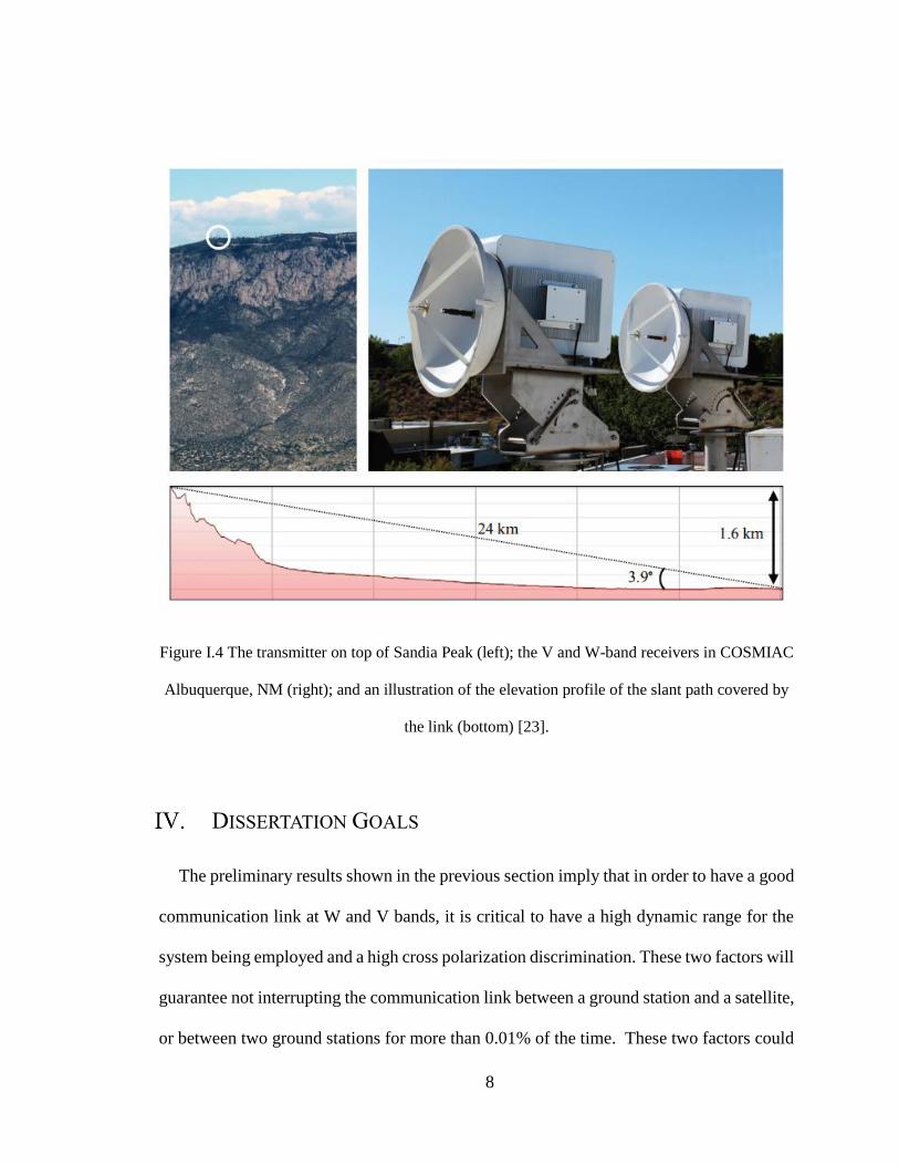
The transmitter is located at Sandia Peak, and the receiver is located on the roof top of

the COSMIAC building in Albuquerque. The transmitter consists of a coherent 72 and 84

GHz continuous wave (CW) beacon with an EIRP of 40 dBm using two lens antennas with

a 3° half-power beam-width (HPBW) and 35 dBi of gain. The receiver has two 0.5 m

Cassegrain reflector antennas with 52 dBi of gain each with one receiving at 72 GHz and

the other at 84 GHz as shown in Figure I.4. The transmitter and receiver electronics are

temperature controlled so that their power performance does not fluctuate. The receiver

has also a tone injected right before the LNA to monitor the overall gain performance of

the receiving system [23].

The receiver has a dynamic range of 70 dB at V-band and 68 dB at W-band. The

polarization of both transmitter and receiver is LHCP. The receiver has a cross polarization

discrimination (XPD) of 13 dB at V-band and 20 dB at W-band. The power measurements

are taken at a 10 Hz rate.

The link extends over a 24 Km with a 3.9° slant angle as shown in Figure I.4. The slant

angle is aimed to represent the direction of arrivals at which satellite communication takes

7

place. The link provides a dynamic range of 70 dB that allows it to study the attenuation

caused by the different weather conditions such as rain, snow, fog, haze and sand storms.

Multiple atmospheric measurement devices are also used to monitor the weather

conditions. At the transmitter side, a disdrometer is installed to measure the rain drop size

distribution and velocity and a weather station is installed with a wind monitor,

temperature, pressure, and relative humidity sensors. At the receiver side, the same

equipment used at the transmitter side are installed in addition to a radiometer that gives

an estimate of the attenuation experienced. Other systems are used to monitor the weather

conditions over the link path. One such system is a NEXRAD that allows locating the areas

where the weather events are taking place and gives a better understanding of the condition

of the link path. Another device that is used is a SODAR in multiple locations under the

link path. All these instruments give a better image of the weather conditions that are

affecting the wave propagation and help better correlating the weather conditions with the

measurements of power and polarization at the receiver side.

Preliminary results show that in heavy rain events with a rain rate of 17.2 mm/hr at the

receiver side, the attenuation of the wave exceeds the dynamic range of the system on all

channels. No significant depolarization is observed during such rain event. However, in a

snow event, wave attenuation is observed, but more significantly, wave depolarization

takes place for both V and W bands. At W band the wave depolarization is more significant,

where the X-polarization power level exceeds the co-polarization power level. At that

particular event Albuquerque experienced 7.6 mm of snow. Another finding of the

experiment shows that clouds have a peak 12-15 dB attenuation effect on the wave but no

depolarization results from that.

8

Figure I.4 The transmitter on top of Sandia Peak (left); the V and W-band receivers in COSMIAC

Albuquerque, NM (right); and an illustration of the elevation profile of the slant path covered by

the link (bottom) [23].

DISSERTATION GOALS

The preliminary results shown in the previous section imply that in order to have a good

communication link at W and V bands, it is critical to have a high dynamic range for the

system being employed and a high cross polarization discrimination. These two factors will

guarantee not interrupting the communication link between a ground station and a satellite,

or between two ground stations for more than 0.01% of the time. These two factors could

9

be achieved by designing antennas that have high gains and high isolation between the Co-

polarization component and the cross-polarization component.

Several antenna designs are illustrated in this dissertation that could be used in

communication links or radar systems at 72 and 84 GHz.

10

LITERATURE REVIEW

Few types of high gain circularly polarized antennas are designed to operate at W-band

frequencies. Some of the commercially available antennas include conical horns, reflector

and lens antennas. In reality, these antennas are not circularly polarized by nature. They

require the integration of a polarizer unit for circular polarization excitation [24],[25].

In this section, a literature review of the different types of antennas and polarization

techniques that could be designed at W/V band to operate in communication links is done.

The literature review targets the design of high gain antennas, or the design of microwave

polarizers that transform the linear polarization of high gain antennas into a circular

polarization.

SLOTTED RECTANGULAR WAVEGUIDES

Slotted rectangular waveguide antennas are known for their high power handling, high

efficiency and their ability to produce high gain while having a flat small size. These types

of antennas can be used in the transmitter side of a satellite communication link. There are

two types of slotted waveguide antennas: leaky wave arrays and standing wave arrays. The

standing wave arrays are narrow band, which makes them a less favorable option in

communication links that are trying to achieve high data rates. The leaky wave

configuration is the better option and it is the one discussed in the text to follow herein.

Circular polarization of slotted waveguides is achieved by appropriately designing

slotted rectangular waveguide arrays. Such structures can be implemented by having tilted

11

slots along the waveguide centerline on the narrow-wall [26], [27]. However, the

implementation of rectangular slots along the waveguide narrow walls is critical at W-

bands since the slot's length is usually larger than the wall width. This requires the slots to

extend to the broad-wall and thus leading to a difficulty in fabrication and a degradation in

the structure radiation performance.

Another approach in the design of circularly polarized waveguide arrays is to place the

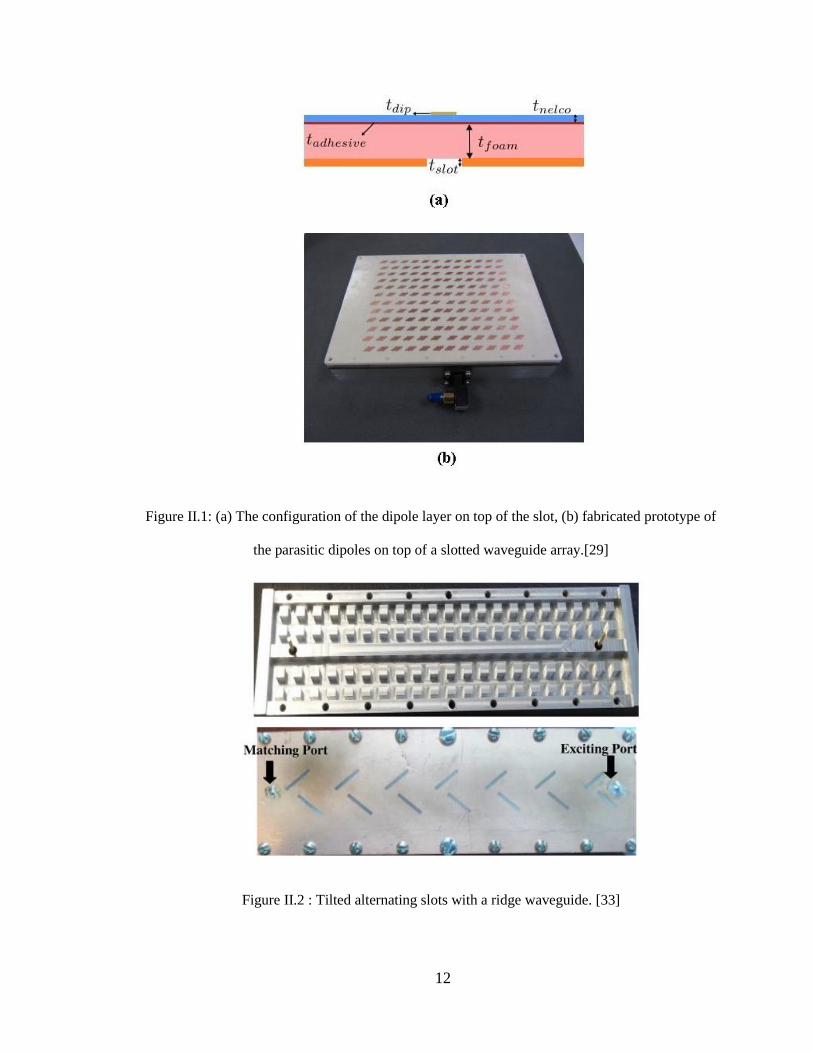
slots on the broad-wall. For example, by adding parasitic dipoles on top of the rectangular

slots of a linearly polarized waveguide array, the polarization can be switched to circular

[28], [29]. This technique reduces the efficiency of the antenna due to the use of a dielectric

material where the parasitic dipoles are fabricated as shown in Figure II.1 (a) and (b).

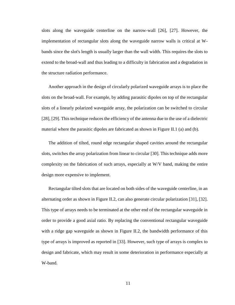
The addition of tilted, round edge rectangular shaped cavities around the rectangular

slots, switches the array polarization from linear to circular [30]. This technique adds more

complexity on the fabrication of such arrays, especially at W/V band, making the entire

design more expensive to implement.

Rectangular tilted slots that are located on both sides of the waveguide centerline, in an

alternating order as shown in Figure II.2, can also generate circular polarization [31], [32].

This type of arrays needs to be terminated at the other end of the rectangular waveguide in

order to provide a good axial ratio. By replacing the conventional rectangular waveguide

with a ridge gap waveguide as shown in Figure II.2, the bandwidth performance of this

type of arrays is improved as reported in [33]. However, such type of arrays is complex to

design and fabricate, which may result in some deterioration in performance especially at

W-band.

12

Figure II.1: (a) The configuration of the dipole layer on top of the slot, (b) fabricated prototype of

the parasitic dipoles on top of a slotted waveguide array.[29]

Figure II.2 : Tilted alternating slots with a ridge waveguide. [33]

13

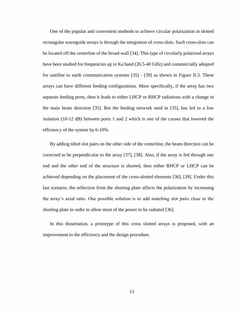
One of the popular and convenient methods to achieve circular polarization in slotted

rectangular waveguide arrays is through the integration of cross-slots. Such cross-slots can

be located off the centerline of the broad-wall [34]. This type of circularly polarized arrays

have been studied for frequencies up to Ka band (26.5-40 GHz) and commercially adopted

for satellite to earth communication systems [35] - [39] as shown in Figure II.3. These

arrays can have different feeding configurations. More specifically, if the array has two

separate feeding ports, then it leads to either LHCP or RHCP radiations with a change in

the main beam direction [35]. But the feeding network used in [35], has led to a low

isolation (10-12 dB) between ports 1 and 2 which is one of the causes that lowered the

efficiency of the system by 6-10%.

By adding tilted slot pairs on the other side of the centerline, the beam direction can be

corrected to be perpendicular to the array [37], [38]. Also, if the array is fed through one

end and the other end of the structure is shorted, then either RHCP or LHCP can be

achieved depending on the placement of the cross-slotted elements [36], [39]. Under this

last scenario, the reflection from the shorting plate affects the polarization by increasing

the array’s axial ratio. One possible solution is to add matching slot pairs close to the

shorting plate in order to allow most of the power to be radiated [36].

In this dissertation, a prototype of this cross slotted arrays is proposed, with an

improvement to the efficiency and the design procedure.

14

Figure II.3: Cross slotted rectangular waveguide array used in satellite communication

transmitter. [39]

WAVEGUIDE POLARIZERS

A waveguide wave polarizer is a microwave device that transforms a linearly polarized

wave at its feeding port into a circularly or elliptically polarized wave at its output port.

They are usually implemented in square or circular waveguides. Multiple techniques are

used to do this transformation that are explained below:

Corrugated waveguide polarizers and Iris Polarizers:

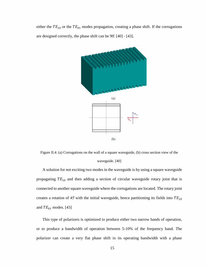
This type of polarizers uses a square waveguide as shown in Figure II.4. In its simplest

form, the 𝑇𝐸10 and the 𝑇𝐸01 modes are excited in the waveguide. The corrugations are on

either the E-plane or the H-plane of the square waveguide. These corrugations will delay

15

either the 𝑇𝐸10 or the 𝑇𝐸01 modes propagation, creating a phase shift. If the corrugations

are designed correctly, the phase shift can be 90. [40] - [43].

Figure II.4: (a) Corrugations on the wall of a square waveguide, (b) cross section view of the

waveguide. [40]

A solution for not exciting two modes in the waveguide is by using a square waveguide

propagating 𝑇𝐸10 and then adding a section of circular waveguide rotary joint that is

connected to another square waveguide where the corrugations are located. The rotary joint

creates a rotation of 45 with the initial waveguide, hence partitioning its fields into 𝑇𝐸10

and 𝑇𝐸01 modes. [43]

This type of polarizers is optimized to produce either two narrow bands of operation,

or to produce a bandwidth of operation between 5-10% of the frequency band. The

polarizer can create a very flat phase shift in its operating bandwidth with a phase

16

difference of 90 - 91. It can either create a left hand circularly polarized (LHCP) wave or

a right hand circularly polarized (RHCP) wave.

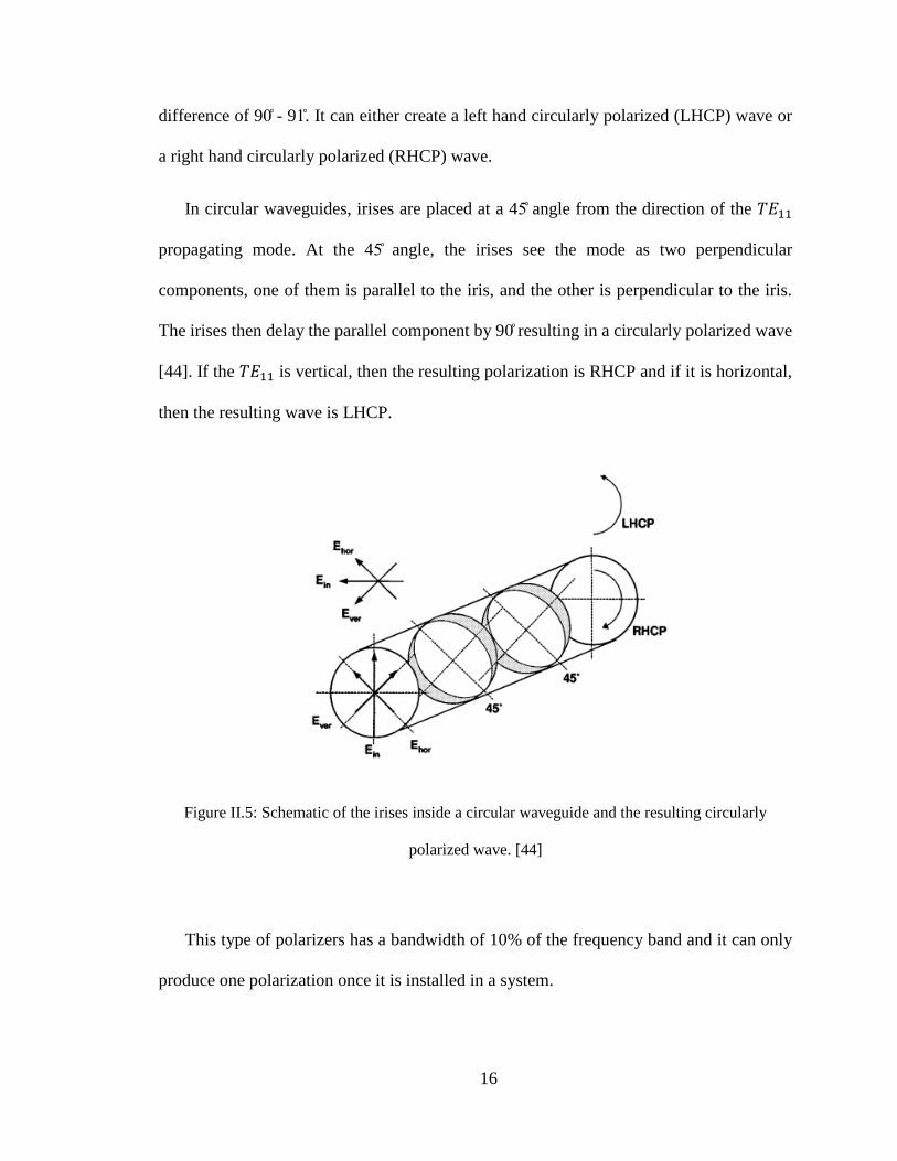
In circular waveguides, irises are placed at a 45 angle from the direction of the 𝑇𝐸11

propagating mode. At the 45 angle, the irises see the mode as two perpendicular

components, one of them is parallel to the iris, and the other is perpendicular to the iris.

The irises then delay the parallel component by 90 resulting in a circularly polarized wave

[44]. If the 𝑇𝐸11 is vertical, then the resulting polarization is RHCP and if it is horizontal,

then the resulting wave is LHCP.

Figure II.5: Schematic of the irises inside a circular waveguide and the resulting circularly

polarized wave. [44]

This type of polarizers has a bandwidth of 10% of the frequency band and it can only

produce one polarization once it is installed in a system.

17

This particular type of polarizers shown in this section are realized at frequencies up to

Ka-band. They are very expensive to achieve at W/V bands because the process of

fabrication is very complicated and requires very high precision.

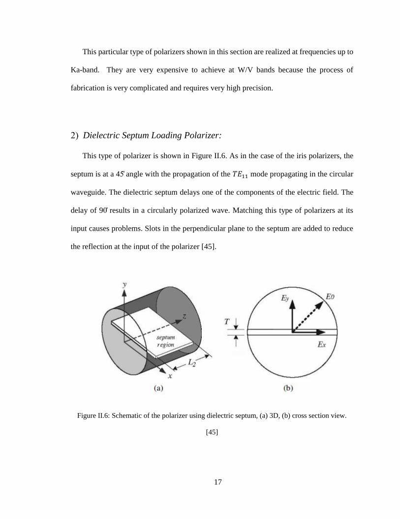
Dielectric Septum Loading Polarizer:

This type of polarizer is shown in Figure II.6. As in the case of the iris polarizers, the

septum is at a 45 angle with the propagation of the 𝑇𝐸11 mode propagating in the circular

waveguide. The dielectric septum delays one of the components of the electric field. The

delay of 90 results in a circularly polarized wave. Matching this type of polarizers at its

input causes problems. Slots in the perpendicular plane to the septum are added to reduce

the reflection at the input of the polarizer [45].

Figure II.6: Schematic of the polarizer using dielectric septum, (a) 3D, (b) cross section view.

[45]

18

This design only results in one polarization sense at the same configuration. It is

realized at 60 GHz with a good performance between 60-62.5 GHz. Other polarizers that

use either dielectric septum or metallic septum are available commercially. These

polarizers can produce a bandwidth of operation that could reach 20% of the frequency

band. [46]

Septum OMT polarizer:

This type of polarizers is a three port network, where the third port has two modes

propagating in it and forming a circularly polarized wave. If the first port is fed, a RHCP

wave is generated at port 3, and if port 2 is fed, a LHCP wave is formed at port 3 as shown

in Figure II.7 [47]-[54].

Figure II.7: Schematic of the septum OMT polarizer showing its operation modes. [54]

This type of polarizers has an isolation of more than 20 dB between ports 1 and 2 and

can produce axial ratio values of less than 1 dB over a frequency band of 15 -18% of the

19

frequency band for low frequencies [47]. These characteristics, make the polarizer a good

device for use in both transmission and reception simultaneously.

The basic model of the septum is a stepped septum that creates high isolation between

ports 1 and 2, while creating two orthogonal modes in the square waveguide output with

90 phase difference between them [47],[48],[49]. In some designs a corrugation is added

in the square waveguide output in order to correct the phase and make it more flat and close

to 90 [50].

An optimization of the model is introduced in [51], [52]. This optimization makes the

stepping also in the thickness of the septum. The designs done are in the Ka-band producing

a good operation bandwidth of 12% of the frequency band. In [51], the design is made

reconfigurable by introducing shorting plates controlled by piezo-motors in order to control

which channel operates at a certain point for transmission as shown in Figure II.8.

Figure II.8: The different modes of operation of the reconfigurable OMT polarizer. [51]

20

This polarizer can also be implemented in circular waveguides without the need of use

of a square to circular waveguide transition [53]. In this particular design, the polarizer is

used to feed a conical horn feeding a reflector antenna.

At high frequencies, due to fabrication inaccuracies, this design can produce a 10%

bandwidth of operation [54]. If used in the WTLE experiment, two of these polarizers are

needed in order to operate at 72GHz and 84 GHz. The Multi-band polarizer, that is

introduced in this dissertation, makes the design simpler, less expensive and operating at

72 and 84 GHz by using the same device.

21

CROSS SLOTTED RECTANGULAR WAVEGUIDE ARRAY

INTRODUCTION

The initial work done at W/V band frequencies is the design of reconfigurable arrays

using liquid crystal in its nematic form. This type of arrays is hard to fabricate, and has low

efficiency at 76 GHz. This work is discussed in Appendix A in more details. For antennas

that are more efficient the work presented hereafter is done.

The implementation of a planar cross-slotted rectangular waveguide array that is

operating with a dual feed is presented here [55], [56]. This type of arrays was used

previously in transmitter systems for satellite communication at lower frequencies (X-band

and Ka-band) [35], [39]. Here the dual feed results in the generation of either RHCP or

LHCP radiations at 84-86 GHz. The integration of z-shaped arm slots on the broad-wall of

the waveguide is also implemented without affecting the total circular polarization

performance and to improve design flexibility and overall radiation efficiency. The new

cross-slot concept, proposed in this work, can be designed for any frequency in the

operating TE10 fundamental mode of the waveguide. In what follows, a detailed description

of the new array design, its fabrication process, and all analytical and experimental results

are presented in details and discussed.

22

DESIGN OF Z-SHAPED CROSS-SLOT

In this section, the design of a z-shaped cross-slot along the broad-wall of a WR-10

rectangular waveguide operating in the TE10 mode is investigated. For the fundamental

mode and along the broad-wall of the waveguide, the magnetic field has two components:

Hx and Hz. As seen from Eq. 1 and Eq. 2, the two components of the magnetic field are 90o

out of phase at all times.

Hx = -A

Z10sin

πx

ae-jβz (III.1)

Hz =jπA

βaZ10cos

πx

ae-jβz (III.2)

At a certain range of positions s, far from the narrow-wall of the waveguide, the

magnitudes of the magnetic field components are equal for certain frequencies [34]. These

positions are given in Eq. 3.

12

1tan

2

1

cfa

as

(III.3)

Circularly polarized waves can therefore be radiated by having a slot centered at a

position s. For each frequency there are two positions s where circular polarization is

achieved. Also, by changing the z-direction in which the wave is propagating, the radiated

wave can be changed from RHCP to LHCP. This is physically done by changing the

feeding in the waveguide from one port to the other port.

In order to radiate the maximum amount of power, a cross- slot is usually adopted.

Figure III.1(a) depicts a conventional cross-slot placed at a distance s away from one of the

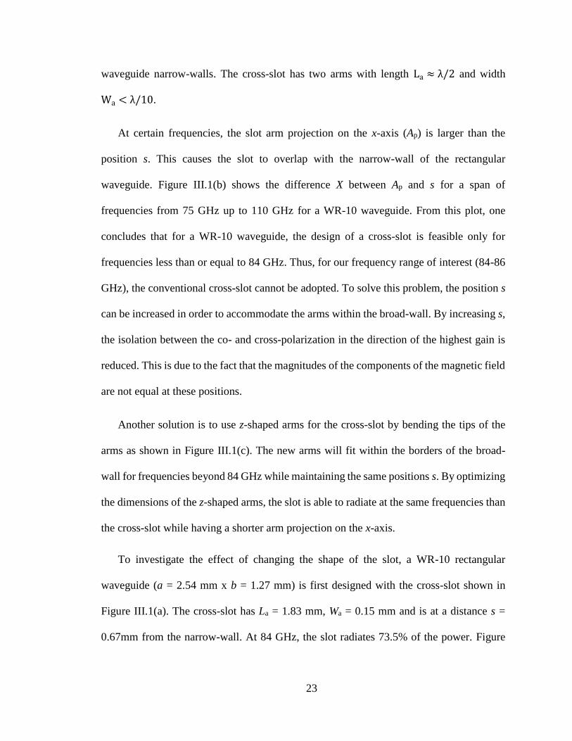
23

waveguide narrow-walls. The cross-slot has two arms with length La ≈ λ/2 and width

Wa < λ/10.

At certain frequencies, the slot arm projection on the x-axis (Ap) is larger than the

position s. This causes the slot to overlap with the narrow-wall of the rectangular

waveguide. Figure III.1(b) shows the difference X between Ap and s for a span of

frequencies from 75 GHz up to 110 GHz for a WR-10 waveguide. From this plot, one

concludes that for a WR-10 waveguide, the design of a cross-slot is feasible only for

frequencies less than or equal to 84 GHz. Thus, for our frequency range of interest (84-86

GHz), the conventional cross-slot cannot be adopted. To solve this problem, the position s

can be increased in order to accommodate the arms within the broad-wall. By increasing s,

the isolation between the co- and cross-polarization in the direction of the highest gain is

reduced. This is due to the fact that the magnitudes of the components of the magnetic field

are not equal at these positions.

Another solution is to use z-shaped arms for the cross-slot by bending the tips of the

arms as shown in Figure III.1(c). The new arms will fit within the borders of the broad-

wall for frequencies beyond 84 GHz while maintaining the same positions s. By optimizing

the dimensions of the z-shaped arms, the slot is able to radiate at the same frequencies than

the cross-slot while having a shorter arm projection on the x-axis.

To investigate the effect of changing the shape of the slot, a WR-10 rectangular

waveguide (a = 2.54 mm x b = 1.27 mm) is first designed with the cross-slot shown in

Figure III.1(a). The cross-slot has La = 1.83 mm, Wa = 0.15 mm and is at a distance s =

0.67mm from the narrow-wall. At 84 GHz, the slot radiates 73.5% of the power. Figure

24

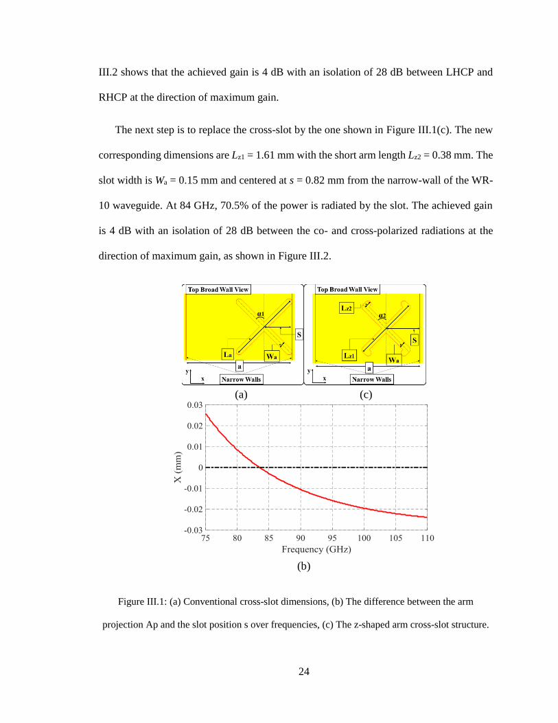
III.2 shows that the achieved gain is 4 dB with an isolation of 28 dB between LHCP and

RHCP at the direction of maximum gain.

The next step is to replace the cross-slot by the one shown in Figure III.1(c). The new

corresponding dimensions are Lz1 = 1.61 mm with the short arm length Lz2 = 0.38 mm. The

slot width is Wa = 0.15 mm and centered at s = 0.82 mm from the narrow-wall of the WR-

10 waveguide. At 84 GHz, 70.5% of the power is radiated by the slot. The achieved gain

is 4 dB with an isolation of 28 dB between the co- and cross-polarized radiations at the

direction of maximum gain, as shown in Figure III.2.

Figure III.1: (a) Conventional cross-slot dimensions, (b) The difference between the arm

projection Ap and the slot position s over frequencies, (c) The z-shaped arm cross-slot structure.

(a)

(b)

(c)

25

Figure III.2: The co- and cross-polarization radiation patterns for the conventional and z-arm slots

in the XZ plane.

Figure III.3: (a) A single WR-10 waveguide element with 4 and 16 slots, (b) The gain variation as

a function of the number of slots.

y

x

(a) (b)

26

The comparison between the two designs at 84 GHz shows that the z-shaped slot

preserves the same polarization isolation as the conventional slot. However, the z-shaped

arm cross-slot ensures that the full slot topology fits on the broad-wall without any overlap

with the narrow-wall for all the frequencies of the W-band.

DESIGN OF A WAVEGUIDE ARRAY

The waveguide topology discussed in Section II exhibits a gain of 4 dB. For the gain

to be improved, an array of slots is introduced along the WR-10 waveguide broad-walls.

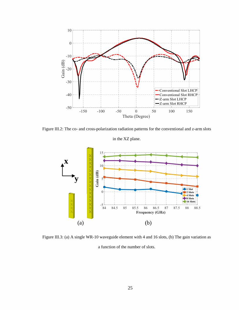
Single Waveguide with Multiple Slots:

The number of z-shaped arm cross-slots determine the maximum gain that can be

produced from a single WR-10 waveguide element. Thus, it is essential to determine the

optimal number of slots that can produce the maximum achievable gain levels. Figure III.3

(a) shows the corresponding structure with 4 and 16 slots. For the different scenarios, the

z-shaped arm cross-slots have the same “long arm” length Lz1 = 1.67 mm and the same

“short arm” length Lz2 = 0.433 mm. The slot width is chosen to be Wa = 0.15 mm and

centered at a distance s = 0.715 mm from the wall of the WR-10 waveguide. The mutual

coupling resulting from introducing several slots in close proximity to each other

necessitates a change in the dimensions of the slots. At first, the waveguide was designed

with 4 slots. The gain exhibited is 8.5 dB at 85 GHz. Doubling the number of slots results

in a gain increase by 2 to 3 dB for operation across the frequency range 84 - 86 GHz. This

can be inspected in Figure III.3(b). The gain reaches 13.5 to 14 dB with N=16 slots. If the

number of slots increases to 32, the increase in gain is only about 0.5-1 dB. Thus, it is found

27

that N=16 slots is a good tradeoff between array size and maximum achievable gain. For

this number of slots, the length of the waveguide is 39.3 mm.

Figure III.4: The co- and cross-polarized radiation patterns at 85.5GHz with N=16 slots in the (a)

elevation (XZ) plane, (b) azimuthal (θ=40o) plane.

The feeding phase difference between the various slots can cause high side lobe levels

if not designed appropriately. Thus, by optimizing the distance of separation between the

slots, the side lobe level can be minimized. A separation distance of Dx = 2.05mm ≈ λ/2

(a)

(b)

28

was determined to be the optimal choice through an iterative analysis. The phase difference

causes the main beam to switch from θ = 0° (one slot) to θ = 40°. Figure III.4(a) shows

the antenna gain pattern for N=16 slots at f=85.5 GHz. It is noticed that the half power

beamwidth (HPBW) in the elevation plane (XZ plane) is 8.7° with an isolation of more than

18 dB between the co- and cross-polarized gain patterns. A drop in the HPBW is achieved

as compared to a single slot due to the increase in the gain levels. The HPBW and isolation

values vary slightly over the entire bandwidth.

Figure III.5: (a) The proposed 8x16 cross-slotted rectangular waveguide array, (b) The gain

variation with the number of waveguides.

The increase in the number of slots in one direction (x-direction) while preserving the

same number in the other direction (y-direction) makes the main beam narrower in one

plane and wider in the other. For example, the HPBW in the azimuthal plane (θ = 40°)

87654321

y

x

Dx

Dy

(a) (b)

Dy

Dx

29

increases to 55o as summarized in Figure III.4(b). One possible solution to maintain almost

the same HPBW along both planes is to transform the proposed structure into a two

dimensional array as detailed next.

2-D Waveguide Array with 16 Slots:

A 2-D array is designed by increasing the number of WR-10 waveguides having 16

slots. The new structure with 8 waveguide elements is shown in Figure III.5(a). The same

slots used in a single waveguide array, are used for the 2-D array. The waveguides of the

2-D array are placed next to each other. All of the waveguides have the cross-slots on the

same side of the wall. The separation between the slots of the same waveguide is kept the

same as in the case of a single waveguide Dx = 2.05mm. The separation between the slots

of the same row in adjacent waveguides is taken to be Dy = 3.04mm. This separation is

limited by the WR-10 waveguide width (a = 2.54 mm) as well as the thickness (𝑡𝑤1 =

0.5 𝑚𝑚) of the walls between any two adjacent waveguides.

The change in the array gain with the increase in the number of the waveguide elements

is plotted in Figure III.5 (b). The gain of the array improves by 2.5 to 3.5 dB as the number

of waveguides is doubled. An increase from around 14 dB to around 24 dB is obtained for

the case of eight waveguides. These results are obtained by forcing all the waveguides in

the simulation environment to be fed in phase and with the same amount of power.

Feeding the various waveguides in phase across the entire frequency band of operation

(84-86 GHz) is a challenging task. The phase effect on the performance of the array is

analyzed with 8 waveguides. If the consecutive waveguides are fed with a constant phase

30

difference ∆ϕin ≠ 0° and with the same amount of power, the main beam of the array

becomes directed in a plane ϕ ≠ 0°. The following four scenarios are investigated:

Case 1:

If the phase difference is 0° < Δ𝜙𝑖𝑛 < 20° between the waveguide elements, the main

beam is entirely circularly polarized and exhibits a gain of 24 dB, with an isolation between

the co- and cross-polarized components of more than 22 dB. The main beam direction is

in a plane 0° < 𝜙 < 5° as shown in Figure III.6.

Case 2:

If the phase difference is 20° < Δ𝜙𝑖𝑛 < 45°, the array produces a main beam with a

gain of 23.5 dB and the isolation between the co- and cross-polarized components is

between 15 and 20 dB. This phase causes circular polarization to be lost across some parts

of the HPBW as shown in Figure III.6.

Case 3:

If the phase difference is ∆ϕin ≥ 45°, the array does not produce a circularly polarized

radiation at the main beam, and the direction of the main beam is in a plane ϕ > 14° as

shown in Figure III.6. In the case of a single slot, the main beam is circularly polarized

along the z-axis. The further away from the z-axis, the less the radiated E-fields are

circularly polarized. The phase difference discussed in this case causes the electric fields

far from the z-axis to add up, and it causes the circularly polarized fields close to the z-axis

to cancel each other. This effect causes the main beam to be elliptically polarized and

directed in a plane ϕ > 14° .

31

Case 4:

In order to direct the main beam in the plane ϕ = 0°, the phase differences between the

consecutive waveguides should be 0° < Δ𝜙𝑖𝑛 < 20°. The various waveguides must also

be fed with the same amount of power. In addition, if the pairs of waveguides (1,8), (2,7),

(3,6) and (4,5), shown in Figure III.5(a), have the same phase at their input then the main

beam is directed in the desired plane.

Figure III.6: The radiation pattern of the array in the azimuthal (θ = 40°) plane for scenarios 1, 2

and 3.

Figure III.7 compares the gain of the array when the various elements are fed in phase

with the case when the phase difference between the elements is 20o. It is found that the

same gain response is obtained. The isolation between the co- and cross-polarized gain

patterns is preserved and the gain is higher than 22 dB in the direction of the highest gain

and over the frequency band of operation. More specifically, the array has the main beam

directed in the plane ϕ = 0° and at an angle θ = 40°. The array’s HPBW is Θ𝑒𝑝 = 8° in

the elevation plane (ϕ = 0°), and Θap = 12.5° in the azimuthal plane (θ = 40°). The

maximum gain achieved is 24 dB over the frequency span of 84-86 GHz.

32

Figure III.7: The gain patterns of the array in the azimuthal (θ = 40°) plane for the case where all

waveguides are fed in phase and for case 4.

FEEDING NETWORK DESIGN

In the previous section, it is concluded that the optimum way to feed the different

waveguide elements is by either having them all fed in phase or by allowing the

symmetrical pairs of waveguides to be fed in phase, and the consecutive waveguides to

have a small phase difference (0° < Δ𝜙𝑖𝑛 < 20°). To achieve this, a separate feeding

network must be designed.

The first proposed feeding network under investigation is depicted in Figure III.8(a). It

is composed of one feeding waveguide that connects directly to the eight WR-10

waveguide elements. The connection is achieved by introducing rectangular slots on the

narrow-wall of the feeding waveguide and shorting its other end. These slots are centered

at the centerline of the narrow-wall and radiate the same power into the eight waveguide

33

elements of the array. The distance of separation between the slots is very crucial on the

array performance since such distance sets the phase difference between the various eight

waveguide elements.

The eight waveguide elements have a center to center separation Dy = 3.04mm. If a

WR-10 rectangular waveguide is used directly as the feeding waveguide, the separation

between the rectangular slots (3.04 mm) results in a ∆𝜙𝑖𝑛 = 223° phase difference

between the consecutive waveguide elements at 85 GHz. This phase difference causes the

main beam to be in the plane 𝜙 = 32°. The gain of the array is reduced to 22 dB and the

circular polarization is lost as shown in Figure III.9. The same behavior is obtained if the

feeding waveguide is a WR-12 rectangular waveguide and the distance of separation

between the rectangular slots is kept to be 3.04 mm. In this case, the phase difference is

∆𝜙𝑖𝑛 = 254.5° at 85 GHz. The main beam is directed in the plane 𝜙 = 37° and the array

is no longer circularly polarized. The gain patterns for this case are also incorporated in

Figure III.9. Based on these results, it is concluded that a transition must exist between the

eight rectangular slots and the opening of the eight WR-10 waveguides.

34

Figure III.8: The proposed feeding with (a) direct connection between the feeding waveguide and

the eight elements WR-10 waveguides, (b) The proposed transition to achieve the required phase

difference between the various elements.

(a)

(b)

Shorting plate

𝑒 𝑝

1 2 3 4 5 6 7 8 𝑒 𝑝

WR12

waveguide

WR10

waveguide

𝑒

WR12

WR10

35

Figure III.9: The gain pattern of the array fed directly by a WR-10 or WR-12 rectangular

waveguide in the azimuthal (θ = 40o) plane.

The modified layout of the proposed feeding network is depicted in Figure III.8(b). For

this case, a WR-12 feeding waveguide with wall thickness 𝑡𝑤2 = 0.5 𝑚𝑚 is adopted since

during measurements, the feeding source has a WR-12 rectangular waveguide output. In

order to achieve a phase difference of ∆ϕin = 0° + 360° between the consecutive

waveguide elements at 85 GHz, the separation between the rectangular slots of the feeding

waveguide should be increased from = 3.04 𝑚𝑚 to = 4.22 𝑚𝑚. The feeding

waveguide is shorted at its other end with a separation of Sshort = 1.71mmbetween the

last slot center and the shorting plate. The rectangular slots have a length Lsf = 1.91mm

and a width Wsf = 0.25mm. These slot dimensions ensure that the feeding network has a

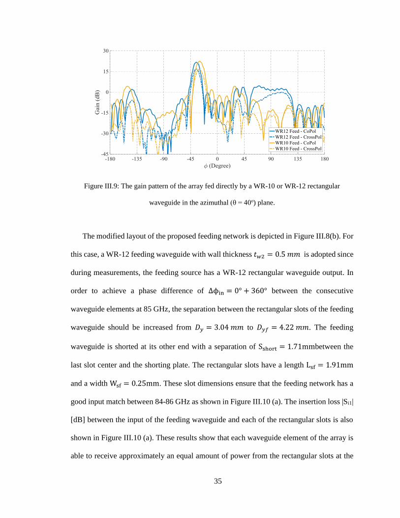
good input match between 84-86 GHz as shown in Figure III.10 (a). The insertion loss |Si1|

[dB] between the input of the feeding waveguide and each of the rectangular slots is also

shown in Figure III.10 (a). These results show that each waveguide element of the array is

able to receive approximately an equal amount of power from the rectangular slots at the

36

frequency bands of operation. The phase difference between the input of the feeding

network and the eight rectangular slots is plotted in Figure III.10 (b). A phase difference in

the range 0° < Δ𝜙𝑖𝑛 < 20° is maintained.

Since the separation distances between the feeding rectangular slots and the

radiating cross-slots are different, serpentine WR-10 rectangular waveguides are used

as shown in Figure III.8(b). The serpentine waveguides are symmetrical for the pairs of

waveguides (1,8), (2,7), (3,6) and (4,5). This design ensures the same phase at the output

of each pair of waveguides and a small phase difference between the consecutive

waveguides. These waveguides are connected to the feeding slots by WR-10 waveguide

sections of length Lext = 5mm in order to minimize the wave reflection caused by the

curvature of the serpentine shape. The serpentine waveguides have a curvature radius

Rserp = 50mm and a total length Lserp = 58.15mm.

Figure III.10: The feeding network S-parameters magnitude in dB and phase in degrees.

37

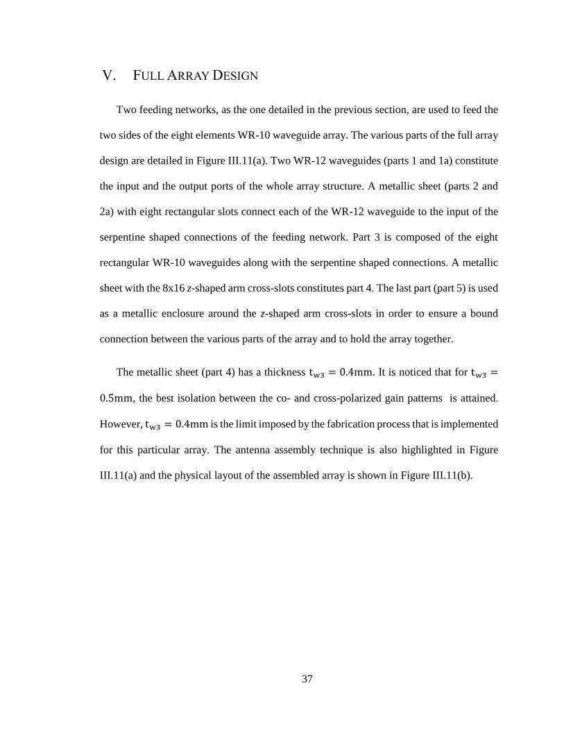
FULL ARRAY DESIGN

Two feeding networks, as the one detailed in the previous section, are used to feed the

two sides of the eight elements WR-10 waveguide array. The various parts of the full array

design are detailed in Figure III.11(a). Two WR-12 waveguides (parts 1 and 1a) constitute

the input and the output ports of the whole array structure. A metallic sheet (parts 2 and

2a) with eight rectangular slots connect each of the WR-12 waveguide to the input of the

serpentine shaped connections of the feeding network. Part 3 is composed of the eight

rectangular WR-10 waveguides along with the serpentine shaped connections. A metallic

sheet with the 8x16 z-shaped arm cross-slots constitutes part 4. The last part (part 5) is used

as a metallic enclosure around the z-shaped arm cross-slots in order to ensure a bound

connection between the various parts of the array and to hold the array together.

The metallic sheet (part 4) has a thickness tw3 = 0.4mm. It is noticed that for tw3 =

0.5mm, the best isolation between the co- and cross-polarized gain patterns is attained.

However, tw3 = 0.4mm is the limit imposed by the fabrication process that is implemented

for this particular array. The antenna assembly technique is also highlighted in Figure

III.11(a) and the physical layout of the assembled array is shown in Figure III.11(b).

38

Figure III.11: The full array design (a) disassembled, (b) assembled and (c) radiation pattern for

each port.

(a)

(b)

Part 1

Part 1a

Part 2

Part 2a

Part 3 Part 4

Part 5

(c)

Port 2 LHCP

Port 1 Port 2

x

z

y

Port 1 RHCP

39

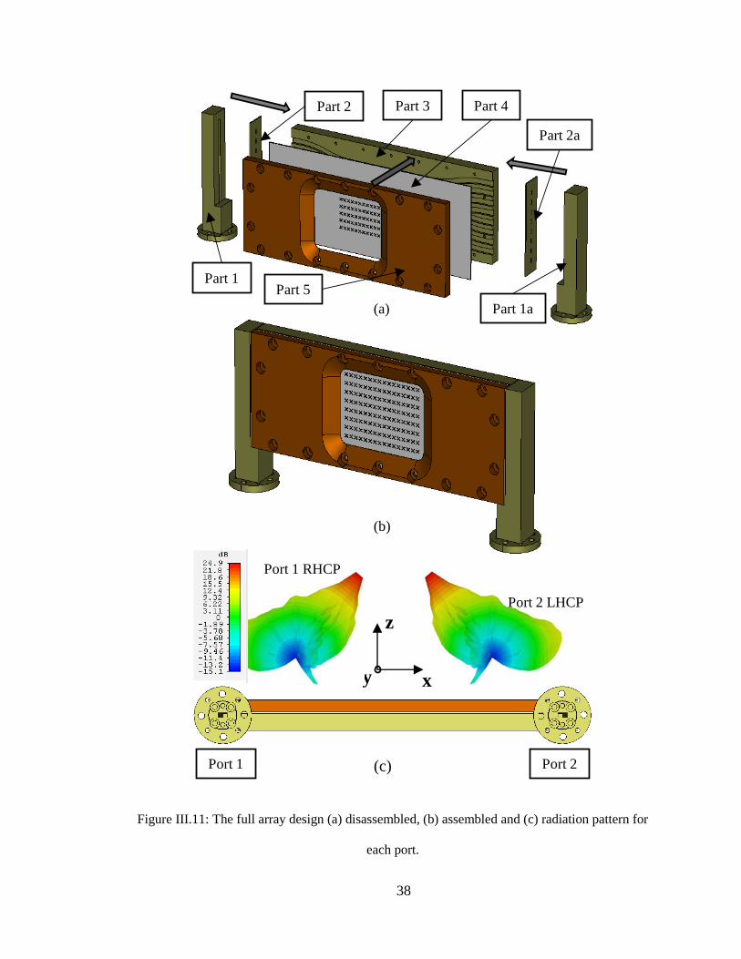
Table III.1: Dimensions of the different parameters of the array.

z-shaped arm cross-slot parameters

Parameter Description Value

𝑧1 long arm length 1.65 mm

𝑧2 short arm length 0.433 mm

𝑎 arm width 0.15 mm

slot center position 0.7 mm

𝛼2 arm angle with y-axis 43°

slots separation along x-axis 2.05 mm

slots separation along y-axis 3.05 mm

𝑡𝑤3 slot thickness 0.4 mm

Feeding Network Parameters


feeding slot length 1.914mm

feeding slot width 0.25mm

feeding slots separation 4.22 mm

last slot center separation with shorting plate 1.71mm

𝑒 𝑝 serpentine waveguide curvature radius 50 mm

𝑒 𝑝 serpentine waveguides length 58.15 mm

𝑡𝑤2 feeding slot thickness 0.5 mm

The final design dimensions are optimized using the CST built-in optimization tool in

order to deliver a gain of 23 - 24 dB over the frequency band of operation (84 – 86 GHz).

The main beam in the elevation plane is directed in θ = 40° when fed through port 1 and

θ = -40° when fed through port 2 as shown in Figure III.11 (c). The final design parameters

are shown in Table III.1. It is essential to note that the feeding network and the metallic

enclosure have no effect on the radiation pattern of the array.

40

MEASURED RESULTS

The entire array structure is fabricated as shown in Figure III.12(a). The antenna

operating bandwidth is 84.1 - 85.8 GHz for port 1, and 84.35-86 GHz for port 2 as depicted

in Figure III.13. The measurement results show an acceptable agreement with the simulated

data. In fact, port 1 exhibits a slightly different yet tolerable performance. The slight

discrepancy is due to some of the fabrication imprecisions (5-10 μm) in terms of milling

the various slots in addition to the assembly misalignment. Both ports share a 1.45 GHz

operating bandwidth extending between 84.35-85.8 GHz. The antenna has a great isolation

between both ports since the measured isolation between the ports is more than 20 dB over

the frequency of operation as shown in Figure III.13.

The antenna’s radiation pattern is measured in the azimuthal (θ = 40°) and elevation

(ϕ = 0°) planes over different frequencies in the operating bandwidth. The measurement

setup for both planes is shown in Figure III.12(b) and (c). A waveguide rotary joint is used

for the azimuthal plane (θ = 40°) measurement. When port 1 is fed, port 2 is loaded with

a WR-12 waveguide matched load and vice versa. The comparison between the simulated

and measured gain patterns at f=85 GHz and when feeding either port 1 or 2 are

summarized in Figure III.14 for the elevation plane (ϕ = 0°) and in Figure III.15 for the

azimuthal plane (θ = 40°). The measured gain patterns at 85 GHz prove that when the

antenna is fed through port 1, it creates a RHCP main beam in the elevation plane in the

direction θ = 40°. When it is fed through port 2, the antenna creates a LHCP main beam

in the elevation plane in the direction θ = -40°. These results show that the change in port

feeding causes the polarization to switch from LHCP to RHCP.

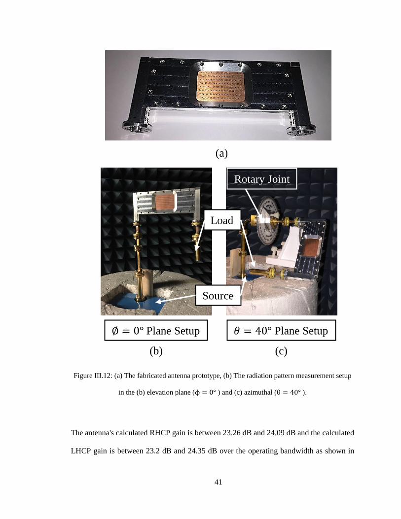
41

Figure III.12: (a) The fabricated antenna prototype, (b) The radiation pattern measurement setup

in the (b) elevation plane (ϕ = 0° ) and (c) azimuthal (θ = 40° ).

The antenna's calculated RHCP gain is between 23.26 dB and 24.09 dB and the calculated

LHCP gain is between 23.2 dB and 24.35 dB over the operating bandwidth as shown in

(a)

(b) (c)

Rotary Joint

Source

Load

𝜃 = 40° Plane Setup = 0° Plane Setup

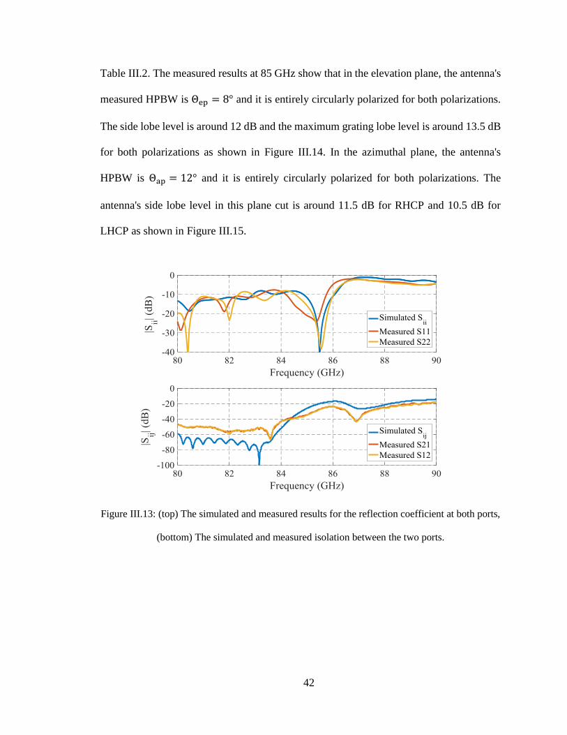
42

Table III.2. The measured results at 85 GHz show that in the elevation plane, the antenna's

measured HPBW is Θep = 8° and it is entirely circularly polarized for both polarizations.

The side lobe level is around 12 dB and the maximum grating lobe level is around 13.5 dB

for both polarizations as shown in Figure III.14. In the azimuthal plane, the antenna's

HPBW is Θap = 12° and it is entirely circularly polarized for both polarizations. The

antenna's side lobe level in this plane cut is around 11.5 dB for RHCP and 10.5 dB for

LHCP as shown in Figure III.15.

Figure III.13: (top) The simulated and measured results for the reflection coefficient at both ports,

(bottom) The simulated and measured isolation between the two ports.

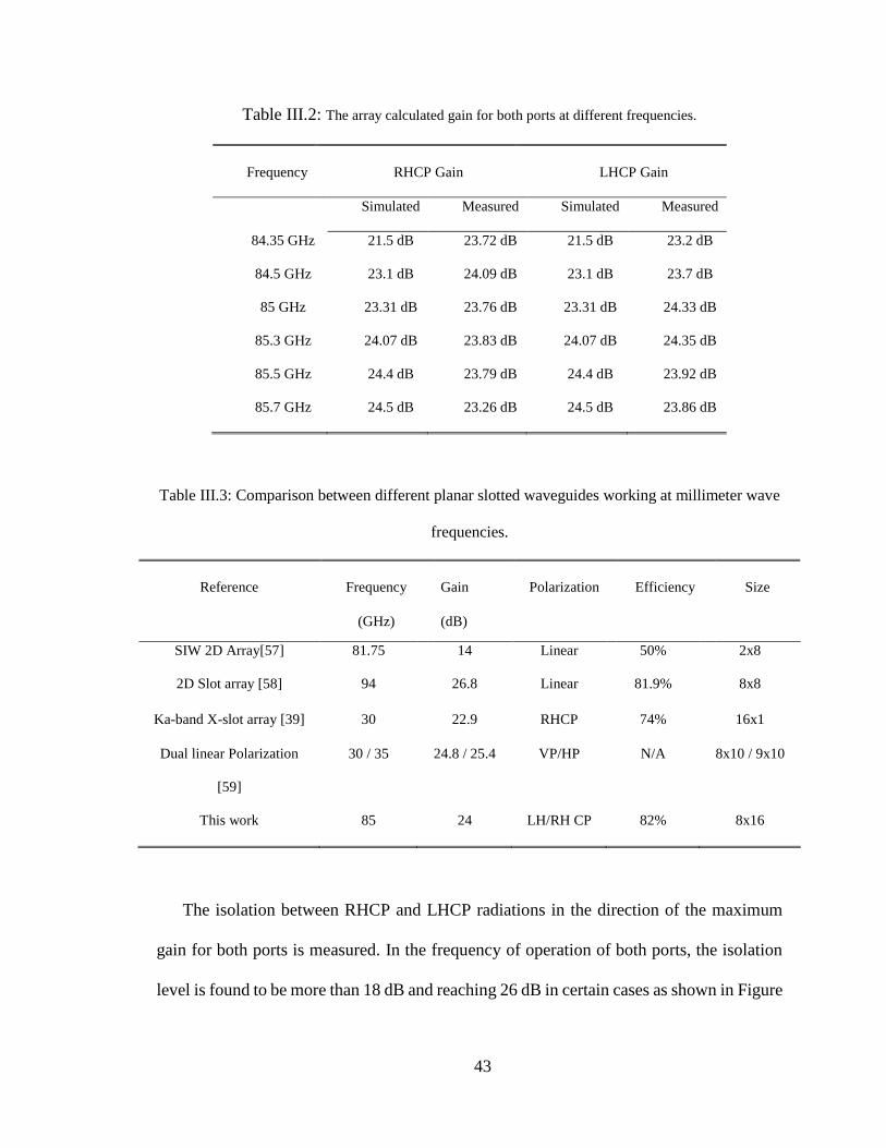
43

Table III.2: The array calculated gain for both ports at different frequencies.

Frequency RHCP Gain LHCP Gain

Simulated Measured Simulated Measured

84.35 GHz 21.5 dB 23.72 dB 21.5 dB 23.2 dB

84.5 GHz 23.1 dB 24.09 dB 23.1 dB 23.7 dB

85 GHz 23.31 dB 23.76 dB 23.31 dB 24.33 dB

85.3 GHz 24.07 dB 23.83 dB 24.07 dB 24.35 dB

85.5 GHz 24.4 dB 23.79 dB 24.4 dB 23.92 dB

85.7 GHz 24.5 dB 23.26 dB 24.5 dB 23.86 dB

Table III.3: Comparison between different planar slotted waveguides working at millimeter wave

frequencies.

Reference Frequency

(GHz)

Gain

(dB)

Polarization Efficiency Size

SIW 2D Array[57] 81.75 14 Linear 50% 2x8

2D Slot array [58] 94 26.8 Linear 81.9% 8x8

Ka-band X-slot array [39] 30 22.9 RHCP 74% 16x1

Dual linear Polarization

[59]

30 / 35 24.8 / 25.4 VP/HP N/A 8x10 / 9x10

This work 85 24 LH/RH CP 82% 8x16

The isolation between RHCP and LHCP radiations in the direction of the maximum

gain for both ports is measured. In the frequency of operation of both ports, the isolation

level is found to be more than 18 dB and reaching 26 dB in certain cases as shown in Figure

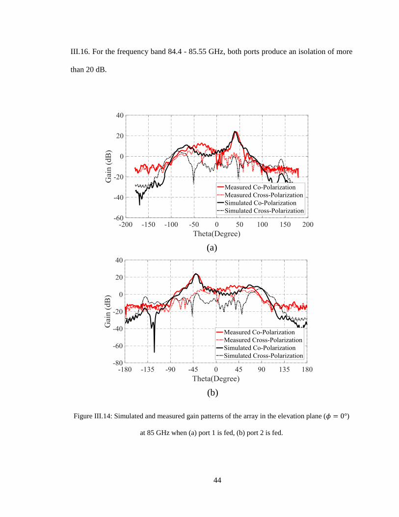
44

III.16. For the frequency band 84.4 - 85.55 GHz, both ports produce an isolation of more

than 20 dB.

Figure III.14: Simulated and measured gain patterns of the array in the elevation plane (𝜙 = 0°)

at 85 GHz when (a) port 1 is fed, (b) port 2 is fed.

(a)

(b)

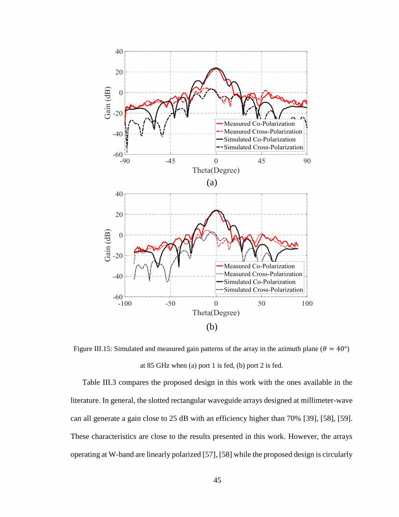
45

Figure III.15: Simulated and measured gain patterns of the array in the azimuth plane (𝜃 = 40°)

at 85 GHz when (a) port 1 is fed, (b) port 2 is fed.

Table III.3 compares the proposed design in this work with the ones available in the

literature. In general, the slotted rectangular waveguide arrays designed at millimeter-wave

can all generate a gain close to 25 dB with an efficiency higher than 70% [39], [58], [59].

These characteristics are close to the results presented in this work. However, the arrays

operating at W-band are linearly polarized [57], [58] while the proposed design is circularly

(a)

(b)

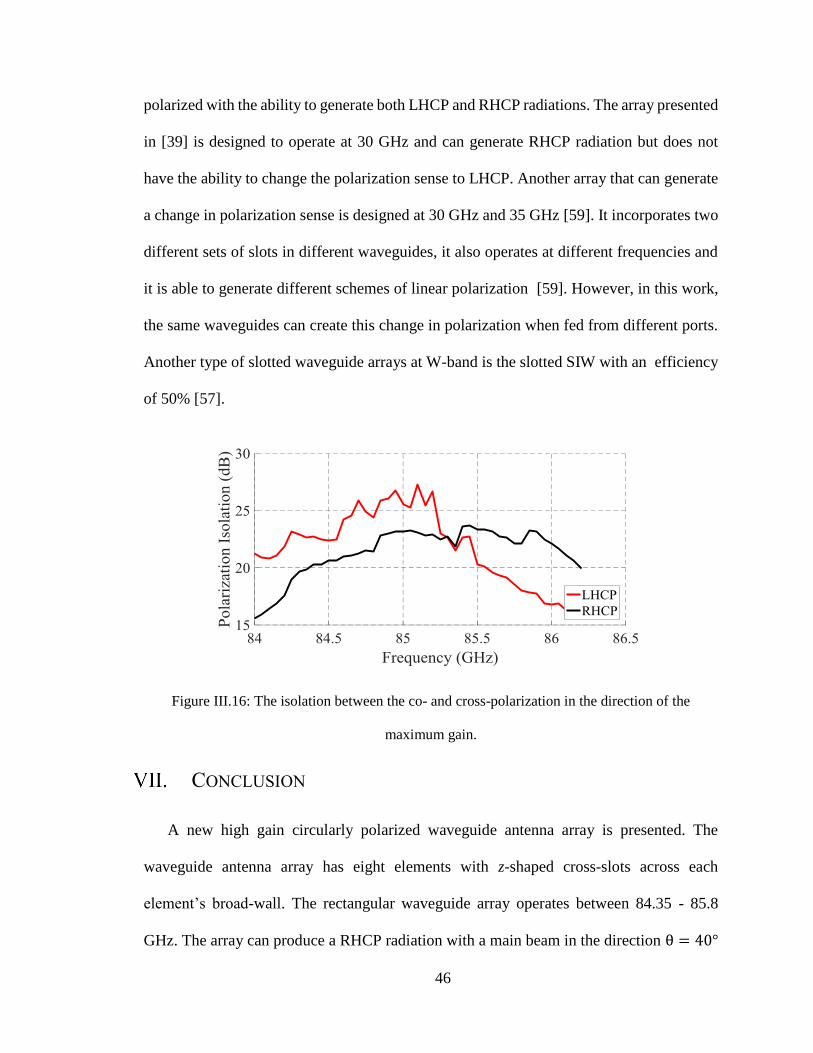
46

polarized with the ability to generate both LHCP and RHCP radiations. The array presented

in [39] is designed to operate at 30 GHz and can generate RHCP radiation but does not

have the ability to change the polarization sense to LHCP. Another array that can generate

a change in polarization sense is designed at 30 GHz and 35 GHz [59]. It incorporates two

different sets of slots in different waveguides, it also operates at different frequencies and

it is able to generate different schemes of linear polarization [59]. However, in this work,

the same waveguides can create this change in polarization when fed from different ports.

Another type of slotted waveguide arrays at W-band is the slotted SIW with an efficiency

of 50% [57].

Figure III.16: The isolation between the co- and cross-polarization in the direction of the

maximum gain.

CONCLUSION

A new high gain circularly polarized waveguide antenna array is presented. The

waveguide antenna array has eight elements with z-shaped cross-slots across each

element’s broad-wall. The rectangular waveguide array operates between 84.35 - 85.8

GHz. The array can produce a RHCP radiation with a main beam in the direction θ = 40°

47

if fed through port 1 and a LHCP radiation with the main beam in the direction θ = -40°

if fed through port 2. The gain achieved for both ports is between 23 and 24.5 dB. The

HPBW has an elliptical shape and is entirely circularly polarized in both elevation and

azimuthal planes. The isolation between the co- and cross-polarized gain patterns in the

direction of the maximum gain is more than 20 dB for both ports. The array is proven to

be a good candidate for point to point terrestrial communication systems as well as satellite

to earth communication systems.

48

CROSS SLOT POLARIZER

I. INTRODUCTION

The array of cross slotted waveguides presented in the previous chapter can generate a

RHCP beam in the direction θ = +40 when fed through port 1, and LHCP beam in the

direction θ = -40 when fed through port 2. This requires the array to be rotated in order

for the two beams to be pointing at the same target. This means that the LHCP and RHCP

properties of the array cannot be used for the same target at the same time. A solution for

this problem is to extract the power from one slot into a waveguide and radiate it into θ =

0 for both LHCP and RHCP radiations. This device can be used as a polarizer for horn

antennas when it is used in the transmitting mode, or it could be used as an orthomode

transducer in the receiving mode. In sections II and III, the theory of a slot radiating into a

circular waveguide is presented and its performance while feeding a conical horn is shown.

Sections IV and V detail the theory of a cross slot radiating into a square waveguide and

feeding a pyramidal horn. Section VI details the design of a serpentine combiner aiming to

improve the performance of a single slot while section VII details the design of a square

waveguide power combiner that improves the performance of the square waveguide

polarizer design. Finally, this chapter concludes with section VIII where the design of multi

band cross slot polarizer systems is illustrated.

49

II. SLOT RADIATING INTO A CIRCULAR WAVEGUIDE

In this section, a slot radiating into a circular waveguide is discussed. The position of

the slot on the broad-wall that excites a circularly polarized wave in a circular waveguide

is derived.

Theory

Let's assume that the slot is located on the broad-wall of the rectangular waveguide

with its center at x = s, y=b and z = 0 as shown in Figure IV.1 (a).

In a rectangular waveguide, the field equations for TE10 mode are:

𝐸 = 𝐴 sin𝜋

𝑎𝑒−𝑗𝛽𝑧 (IV.1)

𝐻 = −𝐴

𝑍10sin

𝜋


𝐻𝑧 = 𝑗𝜋𝐴

𝛽𝑎𝑍10cos

𝜋


where 𝑍10 = 𝑘0𝜂0

𝛽

These fields are shown in Figure IV.1 (b). At the slot, the electric and magnetic

polarizabilities are given by the equations below:

𝑃𝑒 = 𝐴휀0𝛼𝑒 sin𝜋

𝑎𝛿(𝑥 − 𝑠)𝛿(𝑦 − 𝑏)𝛿(𝑧) (IV.4)

𝑃𝑚 = −𝐴𝛼𝑚 [−

𝑍10sin

𝜋

𝑎+

𝑗𝜋

𝛽𝑎𝑍10cos

𝜋

𝑎] 𝛿(𝑥 − 𝑠)𝛿(𝑦 − 𝑏)𝛿(𝑧) (IV.5)

where 𝛼𝑒 and 𝛼𝑚 are constants related to the slot shape and dimensions.

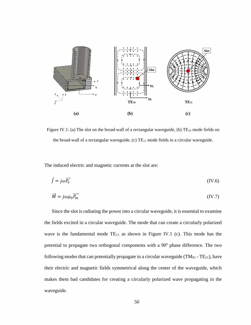
50

Figure IV.1: (a) The slot on the broad-wall of a rectangular waveguide, (b) TE10 mode fields on

the broad-wall of a rectangular waveguide, (c) TE11 mode fields in a circular waveguide.

The induced electric and magnetic currents at the slot are:

𝐽 = 𝑗𝜔𝑃𝑒 (IV.6)

= 𝑗𝜔𝜇0𝑃𝑚 (IV.7)

Since the slot is radiating the power into a circular waveguide, it is essential to examine

the fields excited in a circular waveguide. The mode that can create a circularly polarized

wave is the fundamental mode TE11 as shown in Figure IV.1 (c). This mode has the

potential to propagate two orthogonal components with a 90o phase difference. The two

following modes that can potentially propagate in a circular waveguide (TM01 - TE21), have

their electric and magnetic fields symmetrical along the center of the waveguide, which

makes them bad candidates for creating a circularly polarized wave propagating in the

waveguide.

x

yz a

b

s

(a)

Hx

Hz

TE10

(b)

TE11

(c)

Slot

Slot

51

The fundamental mode TE11 has the following field equations:

𝐸𝑧 = 0 (IV.8)

𝐸𝜌 = −𝑗𝜔𝜇

𝑘𝑐2𝜌[𝐵 cos𝜙 − 𝐶 sin𝜙]𝐽1(𝑘𝑐𝜌)𝑒

−𝑗𝛽𝑧 (IV.9)

𝐸𝜙 = 𝑗𝜔𝜇

𝑘𝑐[𝐵 sin𝜙 + 𝐶 cos𝜙]𝐽1′(𝑘𝑐𝜌)𝑒


𝐻𝑧 = [𝐵 sin𝜙 + 𝐶 cos𝜙]𝐽1(𝑘𝑐𝜌)𝑒−𝑗𝛽𝑧 (IV.11)

𝐻𝜌 = −𝑗𝛽

𝑘𝑐[𝐵 sin𝜙 + 𝐶 cos𝜙]𝐽1′(𝑘𝑐𝜌)𝑒


𝐻𝜙 = −𝑗𝛽

𝑘𝑐2𝜌[𝐵 cos 𝜙 − 𝐶 sin𝜙]𝐽1(𝑘𝑐𝜌)𝑒


These equations are in a coordinate system with the z axis aligned with the central line

of the waveguide. Since the rectangular waveguide fields are in Cartesian coordinates and

the circular waveguide fields are in cylindrical coordinates, a conversion of the circular

waveguide fields to Cartesian is needed:

The circular waveguide fields in the Cartesian coordinate system can be written as

follows:

𝐸𝑧 = 0 (IV.14) 𝐻𝑧 = 𝐻𝑧 (IV.15)

𝐸 = 𝐸𝜌 cos𝜙 − 𝐸𝜙 sin𝜙 (IV.16) 𝐻 = 𝐻𝜌 cos𝜙 − 𝐻𝜙 sin 𝜙 (IV.17)

𝐸 = 𝐸𝜌 sin𝜙 + 𝐸𝜙 cos𝜙 (IV.18) 𝐻 = 𝐻𝜌 sin 𝜙 + 𝐻𝜙 cos𝜙 (IV.19)

with 𝜌 = √𝑥2 + 𝑦2 and 𝜙 = tan−1

This leads to the following field equations:

52

𝐸𝑧 = 0 (IV.20)

𝐸 = − 𝐵𝑗𝜔𝜇

𝑘𝑐[(cos(tan−1

𝑦

𝑥))2

𝑘𝑐√ 2+ 2

𝐽1(𝑘𝑐√𝑥2 + 𝑦2) + (sin (tan−1

))

2𝐽1′(𝑘𝑐√𝑥

2 + 𝑦2)] 𝑒−𝑗𝛽𝑧 +

𝐶𝑗𝜔𝜇

𝑘𝑐[sin (tan−1

) cos (tan−1

)(

𝐽1(𝑘𝑐√ 2+ 2)

𝑘𝑐√ 2+ 2

− 𝐽1′(𝑘𝑐√𝑥2 + 𝑦2))] 𝑒−𝑗𝛽𝑧 (IV.21)

𝐸 =𝑗𝐵𝜔𝜇


) cos (tan−1

) ( 𝐽1

′(𝑘𝑐√𝑥2 + 𝑦2) −

𝐽1(𝑘𝑐√ 2+ 2)

𝑘𝑐√ 2+ 2

)] 𝑒−𝑗𝛽𝑧 +

𝐶𝑗𝜔𝜇

𝑘𝑐[(sin(tan−1

𝑦

𝑥))2

𝑘𝑐√ 2+ 2

𝐽1(𝑘𝑐√𝑥2 + 𝑦2) + (cos (tan−1

))


2 + 𝑦2)] 𝑒−𝑗𝛽𝑧 (IV.22)

𝐻 =𝑗𝛽𝐵


) cos (tan−1

)(

𝐽1(𝑘𝑐√ 2+ 2)

𝑘𝑐√ 2+ 2

− 𝐽1′(𝑘𝑐√𝑥

2 + 𝑦2))] 𝑒−𝑗𝛽𝑧 −

𝑗𝛽𝐶


𝑦

𝑥))2

𝑘𝑐√ 2+ 2

𝐽1(𝑘𝑐√𝑥2 + 𝑦2) + (cos (tan−1

))


2 + 𝑦2)] 𝑒−𝑗𝛽𝑧 (IV.23)

𝐻 = − 𝑗𝛽𝐵


𝑦

𝑥))2

𝑘𝑐√ 2+ 2𝐽1(𝑘𝑐√𝑥2 + 𝑦2) +

(sin (tan−1

))

2

𝐽1′(𝑘𝑐√𝑥2 + 𝑦2)] 𝑒

−𝑗𝛽𝑧 +

𝐶𝑗𝛽


) cos (tan−1

) (

𝐽1(𝑘𝑐√ 2+ 2)

𝑘𝑐√ 2+ 2− 𝐽1′(𝑘𝑐√𝑥2 + 𝑦2))] 𝑒


𝐻𝑧 = [𝐵 sin (tan−1

) + 𝐶 cos (tan−1

)] 𝑒−𝑗𝛽𝑧 (IV.25)

The circular waveguide is centered at x = s, y=b and z = 0. This requires certain

transformations to be applied to the circular waveguide fields in order to match the case being

solved in here and write everything in the initial coordinate system. The resulting fields of

the TE11 mode propagating in the circular waveguide after the transformations are as follows:

53

𝐸 =𝑗𝐵𝜔𝜇


−

𝑧) cos (tan−1

−

𝑧) ( 𝐽1

′(𝑘𝑐√(𝑥 − 𝑠)2 + 𝑧2) −

𝐽1(𝑘𝑐√( − )2+ 𝑧2)

𝑘𝑐√( − )2+ 𝑧2)] 𝑒−𝑗𝛽( −𝑏) +

𝑗𝜔𝜇𝐶


𝑥−𝑠

𝑧))2

𝑘𝑐√( − )2+ 𝑧2𝐽1(𝑘𝑐√(𝑥 − 𝑠)2 + 𝑧2) +

(cos (tan−1 −

𝑧))

2

𝐽1′(𝑘𝑐√(𝑥 − 𝑠)2 + 𝑧2)] 𝑒−𝑗𝛽( −𝑏) (IV.26)

𝐸 = 0 (IV.27)

𝐸𝑧 = − 𝐵𝑗𝜔𝜇


𝑥−𝑠

𝑧))2

𝑘𝑐√( − )2+ 𝑧2𝐽1(𝑘𝑐√(𝑥 − 𝑠)2 + 𝑧2) +

(sin (tan−1 −

𝑧))

2

𝐽1′(𝑘𝑐√(𝑥 − 𝑠)2 + 𝑧2)] 𝑒−𝑗𝛽( −𝑏) +

𝐶𝑗𝜔𝜇


−

𝑧) cos (tan−1

−

𝑧) (

𝐽1(𝑘𝑐√( − )2+ 𝑧2)

𝑘𝑐√( − )2+ 𝑧2−

𝐽1′(𝑘𝑐√(𝑥 − 𝑠)2 + 𝑧2))] 𝑒−𝑗𝛽( −𝑏) (IV.28)

𝐻 = − 𝑗𝛽𝐵


𝑥−𝑠

𝑧))2

𝑘𝑐√( − )2+ 𝑧2𝐽1(𝑘𝑐√(𝑥 − 𝑠)2 + 𝑧2) +

(sin (tan−1 −

𝑧))

2

𝐽1′(𝑘𝑐√(𝑥 − 𝑠)2 + 𝑧2)] 𝑒−𝑗𝛽( −𝑏) +

𝐶𝑗𝛽


−

𝑧) cos (tan−1

−

𝑧) (

𝐽1(𝑘𝑐√( − )2+ 𝑧2)

𝑘𝑐√( − )2+ 𝑧2−

𝐽1′(𝑘𝑐√(𝑥 − 𝑠)2 + 𝑧2))] 𝑒−𝑗𝛽( −𝑏) (IV.29)

𝐻 = [𝐵 sin (tan−1 −

𝑧) + 𝐶 cos (tan−1

−

𝑧)] 𝑒−𝑗𝛽( −𝑏) (IV.30)

54

𝐻𝑧 =𝑗𝛽𝐵


−

𝑧) cos (tan−1

−

𝑧) (

𝐽1(𝑘𝑐√( − )2+ 𝑧2)

𝑘𝑐√( − )2+ 𝑧2−

𝐽1′(𝑘𝑐√(𝑥 − 𝑠)2 + 𝑧2))] 𝑒−𝑗𝛽( −𝑏) −

𝑗𝛽𝐶


𝑥−𝑠

𝑧))2

𝑘𝑐√( − )2+ 𝑧2𝐽1(𝑘𝑐√(𝑥 − 𝑠)2 + 𝑧2) +

(cos (tan−1 −

𝑧))

2

𝐽1′(𝑘𝑐√(𝑥 − 𝑠)2 + 𝑧2)] 𝑒−𝑗𝛽( −𝑏) (IV.31)

Since the magnitude of the components of the E-field are important in creating a

circularly polarized wave, B and C should be calculated. In order to get B and C, the

following equations are solved:

𝐵 = 1

𝑃11∫ 𝐸1 . 𝐽 𝑑𝑣

𝑣−

1

𝑃11∫ 𝐻1 . 𝑑𝑣

𝑣 (IV.32)

𝐶 = 1

𝑃11∫ 𝐸2 . 𝐽 𝑑𝑣

𝑣−

1

𝑃11∫ 𝐻2 . 𝑑𝑣

𝑣 (IV.33)

In this case:

. 𝐽 = 0 and . is non-zero.

This leads the expressions of B and C to be reduced to the following:

𝐵 = 𝐻1 (𝑠, 𝑏, 0) × 𝑀 + 𝐻1𝑧(𝑠, 𝑏, 0) × 𝑀𝑧 (IV.34)

𝐶 = 𝐻2 (𝑠, 𝑏, 0) × 𝑀 + 𝐻2𝑧(𝑠, 𝑏, 0) × 𝑀𝑧 (IV.35)

where:

𝐻1 = − 𝑗𝛽


𝑥−𝑠

𝑧))2

𝑘𝑐√( − )2+ 𝑧2𝐽1(𝑘𝑐√(𝑥 − 𝑠)2 + 𝑧2) +

(sin (tan−1 −

𝑧))

2

𝐽1′(𝑘𝑐√(𝑥 − 𝑠)2 + 𝑧2)] 𝑒−𝑗𝛽( −𝑏) (IV.36)

55

𝐻2 =𝑗𝛽


−

𝑧) cos (tan−1

−

𝑧) (

𝐽1(𝑘𝑐√( − )2+ 𝑧2)

𝑘𝑐√( − )2+ 𝑧2−

𝐽1′(𝑘𝑐√(𝑥 − 𝑠)2 + 𝑧2))] 𝑒−𝑗𝛽( −𝑏) (IV.37)

𝐻1𝑧 =𝑗𝛽


−

𝑧) cos (tan−1

−

𝑧) (

𝐽1(𝑘𝑐√( − )2+ 𝑧2)

𝑘𝑐√( − )2+ 𝑧2−

𝐽1′(𝑘𝑐√(𝑥 − 𝑠)2 + 𝑧2))] 𝑒−𝑗𝛽( −𝑏) (IV.38)

𝐻2𝑧 = −𝑗𝛽


𝑥−𝑠

𝑧))2

𝑘𝑐√( − )2+ 𝑧2𝐽1(𝑘𝑐√(𝑥 − 𝑠)2 + 𝑧2) +

(cos (tan−1 −

𝑧))

2

𝐽1′(𝑘𝑐√(𝑥 − 𝑠)2 + 𝑧2)] 𝑒−𝑗𝛽( −𝑏) (IV.39)

To simplify these expressions, the small argument approximation for the Bessel function

is used:

𝐽1(𝑙) = 𝑙

2

𝐽1′(𝑙) =

1

2

These approximations stand because, in this scenario, the Bessel function is being

evaluated in the proximity of zero. The resulting simplified fields are as follows:

𝐻1 (𝑠, 𝑏, 0) = − 𝑗𝛽


𝑥−𝑠

𝑧))2

2+ (sin (tan−1

−

𝑧))

2 1

2)] = −

𝑗𝛽

2𝑘𝑐 (IV.40)

𝐻2 (𝑠, 𝑏, 0) =𝑗𝛽


−

𝑧) cos (tan−1

−

𝑧) (

1

2−

1

2 )] = 0 (IV.41)

56

𝐻1𝑧(𝑠, 𝑏, 0) =𝑗𝛽


−

𝑧) cos (tan−1

−

𝑧) (

1

2−

1

2 )] = 0 (IV.42)

𝐻2𝑧(𝑠, 𝑏, 0) = −𝑗𝛽


𝑥−𝑠

𝑧))2

2+ (cos (tan−1

−

𝑧))

2 1

2] = −

𝑗𝛽

2𝑘𝑐 (IV.43)

Solving for B and C using the simplified expressions leads to the following equations:

𝐵 = −𝛽𝜔𝜇0𝛼𝑚𝐴

𝑃11𝑘𝑐𝑍10sin

𝜋

𝑎 (IV.44)

𝐶 =𝑗𝜔𝜇0𝛼𝑚𝐴𝜋

𝑃11𝑎𝑍10𝑘𝑐cos

𝜋

𝑎 (IV.45)

In order to get circular polarization, we need |B| = |C| and ∠𝐵 = ∠𝐶 ±𝜋

2. The

expressions of B and C show that B is real and C is imaginary. This means that they are

90 out of phase, hence satisfying the phase condition.

In order for |B| = |C|, the following should be satisfied:

|−𝛽𝜔𝜇0𝛼𝑚𝐴

𝑃11𝑘𝑐𝑍10sin

𝜋𝑠

𝑎| = |

𝑗𝜔𝜇0𝛼𝑚𝐴𝜋

𝑃11𝑎𝑍10𝑘𝑐cos

𝜋𝑠

𝑎|

⇒ tan

𝜋𝑠

𝑎=

𝜋

𝛽𝑎

Hence,

𝑠 =𝑎

2 ±

𝑎

𝜋tan−1√(

2 𝑎

𝑐)2 − 1 (IV.46)

Design

In order to verify the theoretical calculations presented in the previous section, a WR-

12 rectangular waveguide with width 𝑎 = 3.1 𝑚𝑚 and height 𝑏 = 1.55 𝑚𝑚 is used with

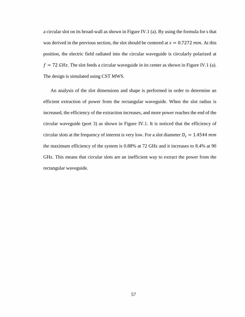
57

a circular slot on its broad-wall as shown in Figure IV.1 (a). By using the formula for s that

was derived in the previous section, the slot should be centered at 𝑠 = 0.7272 𝑚𝑚. At this

position, the electric field radiated into the circular waveguide is circularly polarized at

𝑓 = 72 𝐺𝐻𝑧. The slot feeds a circular waveguide in its center as shown in Figure IV.1 (a).

The design is simulated using CST MWS.

An analysis of the slot dimensions and shape is performed in order to determine an

efficient extraction of power from the rectangular waveguide. When the slot radius is

increased, the efficiency of the extraction increases, and more power reaches the end of the

circular waveguide (port 3) as shown in Figure IV.1. It is noticed that the efficiency of

circular slots at the frequency of interest is very low. For a slot diameter = 1.4544 𝑚𝑚

the maximum efficiency of the system is 0.88% at 72 GHz and it increases to 8.4% at 90

GHz. This means that circular slots are an inefficient way to extract the power from the

rectangular waveguide.

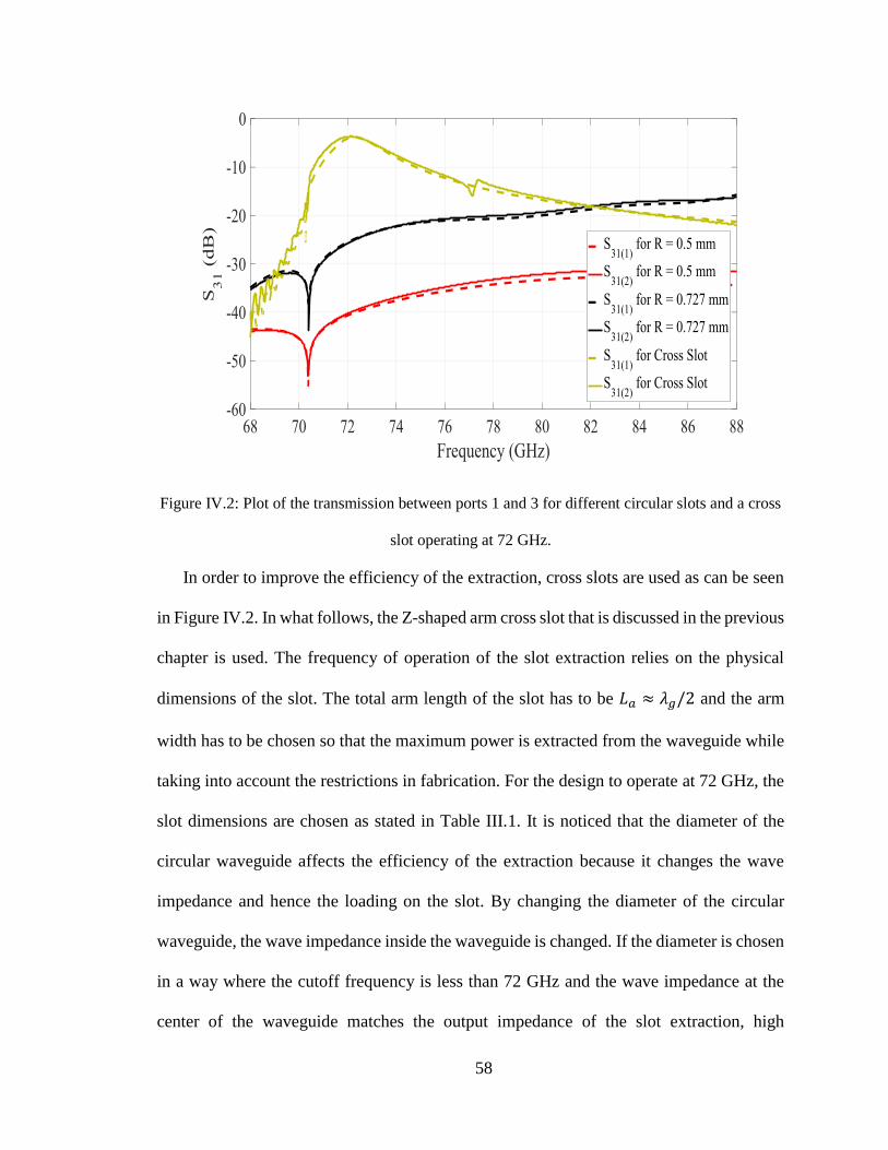
58

Figure IV.2: Plot of the transmission between ports 1 and 3 for different circular slots and a cross

slot operating at 72 GHz.

In order to improve the efficiency of the extraction, cross slots are used as can be seen

in Figure IV.2. In what follows, the Z-shaped arm cross slot that is discussed in the previous

chapter is used. The frequency of operation of the slot extraction relies on the physical

dimensions of the slot. The total arm length of the slot has to be 𝑎 ≈ 𝜆𝑔/2 and the arm

width has to be chosen so that the maximum power is extracted from the waveguide while

taking into account the restrictions in fabrication. For the design to operate at 72 GHz, the

slot dimensions are chosen as stated in Table III.1. It is noticed that the diameter of the

circular waveguide affects the efficiency of the extraction because it changes the wave

impedance and hence the loading on the slot. By changing the diameter of the circular

waveguide, the wave impedance inside the waveguide is changed. If the diameter is chosen

in a way where the cutoff frequency is less than 72 GHz and the wave impedance at the

center of the waveguide matches the output impedance of the slot extraction, high

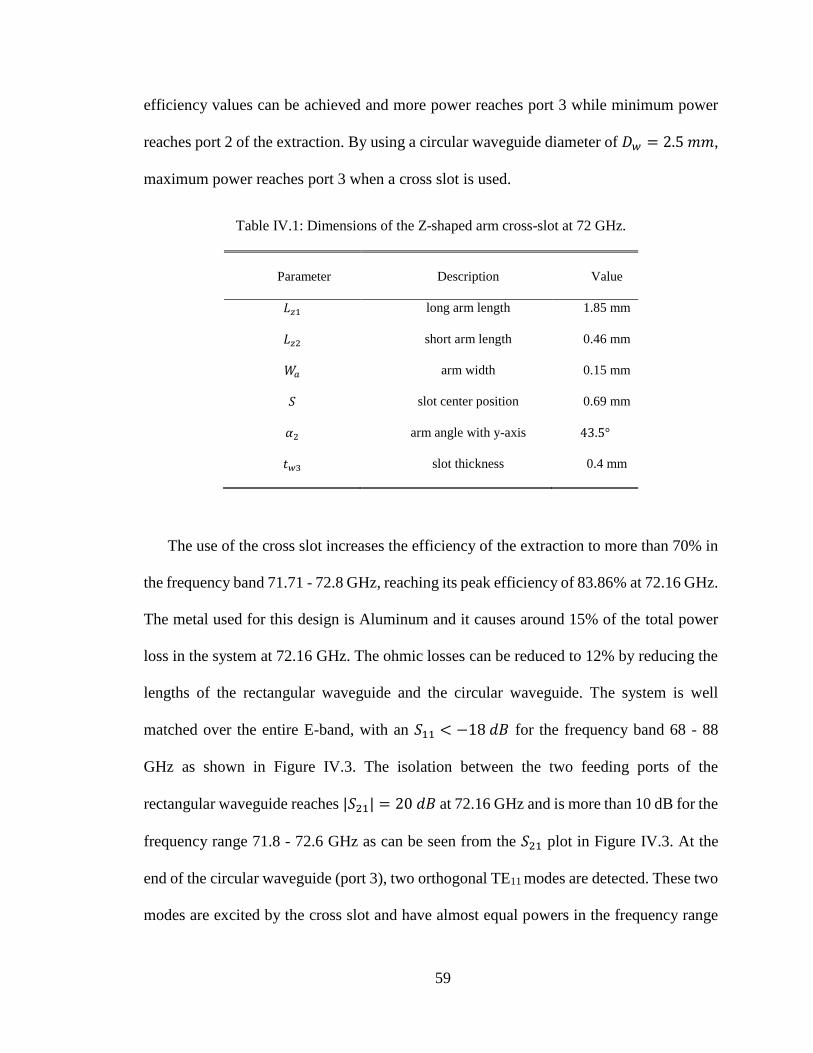
59

efficiency values can be achieved and more power reaches port 3 while minimum power

reaches port 2 of the extraction. By using a circular waveguide diameter of 𝑤 = 2.5 𝑚𝑚,

maximum power reaches port 3 when a cross slot is used.

Table IV.1: Dimensions of the Z-shaped arm cross-slot at 72 GHz.






𝛼2 arm angle with y-axis 43.5°


The use of the cross slot increases the efficiency of the extraction to more than 70% in

the frequency band 71.71 - 72.8 GHz, reaching its peak efficiency of 83.86% at 72.16 GHz.

The metal used for this design is Aluminum and it causes around 15% of the total power

loss in the system at 72.16 GHz. The ohmic losses can be reduced to 12% by reducing the

lengths of the rectangular waveguide and the circular waveguide. The system is well

matched over the entire E-band, with an 11 < −18 𝑑𝐵 for the frequency band 68 - 88

GHz as shown in Figure IV.3. The isolation between the two feeding ports of the

rectangular waveguide reaches | 21| = 20 𝑑𝐵 at 72.16 GHz and is more than 10 dB for the

frequency range 71.8 - 72.6 GHz as can be seen from the 21 plot in Figure IV.3. At the

end of the circular waveguide (port 3), two orthogonal TE11 modes are detected. These two

modes are excited by the cross slot and have almost equal powers in the frequency range

60

71.5 - 88 GHz as seen in the | 31| plot in Figure IV.4. However, the power received by

port 3 is not flat for the entire frequency range. At least half of the power fed through port

1 is received by port 3 in the frequency range 71.43 - 73.35 GHz. The maximum power

that can be received by port 3 coming from port 1 is at 72.16 GHz where | 31(1)| =

−3.88 𝑑𝐵 and | 31(2)| = −3.67 𝑑𝐵. The phase difference between 31(1) and 31(2) is in

the range of 89° < ∠ 31(2) − ∠ 31(1) < 95.4° in the frequency range 71 - 74 GHz as

shown in Figure IV.5.

These results show that this device can work as a wave polarizer with an efficiency of

more than 70% for the frequency range of 71.71 - 72.6 GHz with an isolation between the

two feeding ports of more than 10 dB. The polarizer will create a LHCP wave in the circular

waveguide if fed by port 1, and a RHCP wave if fed by port 2. If both ports 1 and 2 are fed

with equal powers, the resulting wave is linearly polarized. In the next section, the testing

of this device with a horn antenna is illustrated.

Figure IV.3: Plot of the S11 and S21 over frequency for the Z-arm shape cross slot extraction.

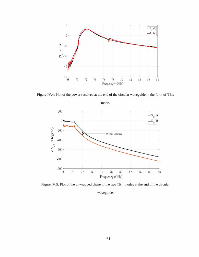
61

Figure IV.4: Plot of the power received at the end of the circular waveguide in the form of TE11

mode.

Figure IV.5: Plot of the unwrapped phase of the two TE11 modes at the end of the circular

waveguide.

62

III. A SINGLE SLOT FEEDING A CONICAL HORN ANTENNA

In order to test its performance, a polarizer is used to feed a horn antenna that can

radiate a circularly polarized wave. Two versions of the polarizer at 72 GHz and 84 GHz

are designed and modified to be matched with the input of the conical horn.

Horn Antenna Design

In order to test the polarizer, a conical horn antenna is used. This antenna has a

symmetrical nature that allows it to support a circularly polarized wave. A polarizer is used

to excite two TE11 modes with orthogonal electric fields at the feeding waveguide input

with a phase difference of 900.

The design of conical horns should follow the guidelines set by A. P. King in [60].

These guidelines determine an optimum horn line that will lead to the best gains of the

horn. This line identifies the best gain that could be achieved as a function of different horn

aperture diameters, for different horn lengths L. The horn parameters L and 𝑑𝑚 along with

the optimum gain achieved are illustrated in Figure IV.6. A numerical equation relating the

optimum directivity of the horn to its geometrical dimensions is also derived and a

relationship between directivity 𝑐, horn length L and aperture diameter 𝑑𝑚 is established

leading to the following equations [61]:

( 𝑐) 𝑝 ≈ 15.9749 (𝐿

𝜆) + 1.7209 (IV.47)

and

≈ 0.3232 (𝑑𝑚

𝜆)2

− 0.0475 (𝑑𝑚

𝜆) + 0.0052 (IV.48)

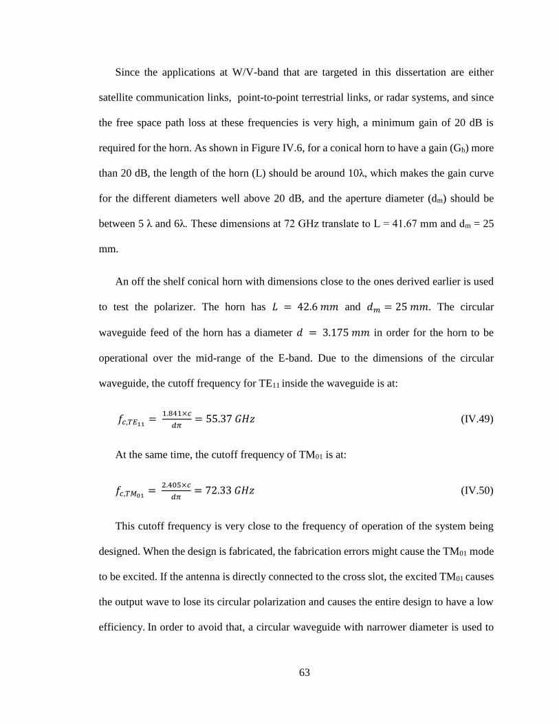
63

Since the applications at W/V-band that are targeted in this dissertation are either

satellite communication links, point-to-point terrestrial links, or radar systems, and since

the free space path loss at these frequencies is very high, a minimum gain of 20 dB is

required for the horn. As shown in Figure IV.6, for a conical horn to have a gain (Gh) more

than 20 dB, the length of the horn (L) should be around 10λ, which makes the gain curve

for the different diameters well above 20 dB, and the aperture diameter (dm) should be

between 5 λ and 6λ. These dimensions at 72 GHz translate to L = 41.67 mm and dm = 25

mm.

An off the shelf conical horn with dimensions close to the ones derived earlier is used

to test the polarizer. The horn has = 42.6 𝑚𝑚 and 𝑑𝑚 = 25 𝑚𝑚. The circular

waveguide feed of the horn has a diameter 𝑑 = 3.175 𝑚𝑚 in order for the horn to be

operational over the mid-range of the E-band. Due to the dimensions of the circular

waveguide, the cutoff frequency for TE11 inside the waveguide is at:

𝑓𝑐,𝑇𝐸11 = 1.841×𝑐

𝑑𝜋= 55.37 𝐺𝐻𝑧 (IV.49)

At the same time, the cutoff frequency of TM01 is at:

𝑓𝑐,𝑇𝑀01=

2.405×𝑐

𝑑𝜋= 72.33 𝐺𝐻𝑧 (IV.50)

This cutoff frequency is very close to the frequency of operation of the system being

designed. When the design is fabricated, the fabrication errors might cause the TM01 mode

to be excited. If the antenna is directly connected to the cross slot, the excited TM01 causes

the output wave to lose its circular polarization and causes the entire design to have a low

efficiency. In order to avoid that, a circular waveguide with narrower diameter is used to

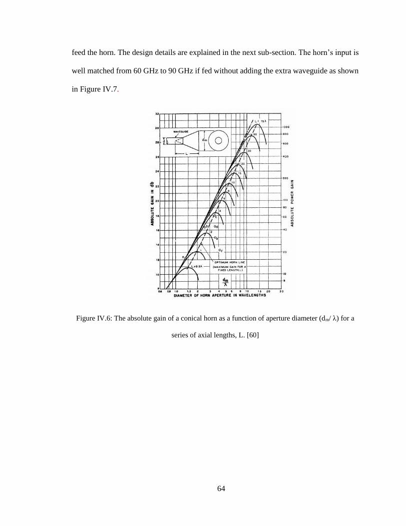
64

feed the horn. The design details are explained in the next sub-section. The horn’s input is

well matched from 60 GHz to 90 GHz if fed without adding the extra waveguide as shown

in Figure IV.7.

Figure IV.6: The absolute gain of a conical horn as a function of aperture diameter (dm/ λ) for a

series of axial lengths, L. [60]

65

Figure IV.7: Conical horn reflection coefficient.

Full System Design

The conical horn is fed using the cross polarizer as shown in Figure IV.8. In order to

suppress higher order modes and only propagate the fundamental TE11 mode inside the

circular waveguide feed of the horn, another circular waveguide with a narrower diameter

is added between the cross slot and the horn system. This new waveguide plays a dual role

of making the extraction of power from the rectangular waveguide more efficient, and

limiting the modes being fed to the conical horn.

In order to have a good matching in the system and good efficiency, a transition

between the two circular waveguides is added. The transition is made of a tapered circular

waveguide. Two different designs, one at 72 GHz and one at 84 GHz are done. The 72

GHz design has a cross slot on the broad-wall of a WR-12 waveguide (a = 3.1 mm and

b=1.55 mm), while the 84 GHz design has the cross slot on the broad-wall of a WR-10

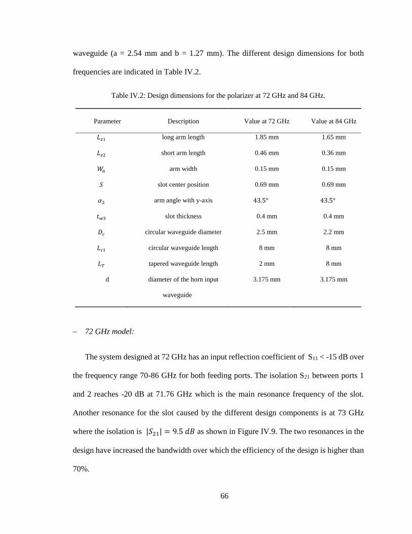
66

waveguide (a = 2.54 mm and b = 1.27 mm). The different design dimensions for both

frequencies are indicated in Table IV.2.

Table IV.2: Design dimensions for the polarizer at 72 GHz and 84 GHz.

Parameter Description Value at 72 GHz Value at 84 GHz

𝑧1 long arm length 1.85 mm 1.65 mm

𝑧2 short arm length 0.46 mm 0.36 mm

𝑎 arm width 0.15 mm 0.15 mm

slot center position 0.69 mm 0.69 mm

𝛼2 arm angle with y-axis 43.5° 43.5°

𝑡𝑤3 slot thickness 0.4 mm 0.4 mm

𝑐 circular waveguide diameter 2.5 mm 2.2 mm

𝑐1 circular waveguide length 8 mm 8 mm

𝑇 tapered waveguide length 2 mm 8 mm

d diameter of the horn input

waveguide

3.175 mm 3.175 mm

72 GHz model:

The system designed at 72 GHz has an input reflection coefficient of S11 < -15 dB over

the frequency range 70-86 GHz for both feeding ports. The isolation S21 between ports 1

and 2 reaches -20 dB at 71.76 GHz which is the main resonance frequency of the slot.

Another resonance for the slot caused by the different design components is at 73 GHz

where the isolation is | 21| = 9.5 𝑑𝐵 as shown in Figure IV.9. The two resonances in the

design have increased the bandwidth over which the efficiency of the design is higher than

70%.

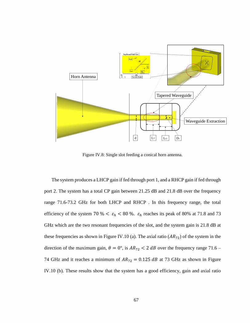
67

Figure IV.8: Single slot feeding a conical horn antenna.

The system produces a LHCP gain if fed through port 1, and a RHCP gain if fed through

port 2. The system has a total CP gain between 21.25 dB and 21.8 dB over the frequency

range 71.6-73.2 GHz for both LHCP and RHCP . In this frequency range, the total

efficiency of the system 70 % < 휀 < 80 %. 휀 reaches its peak of 80% at 71.8 and 73

GHz which are the two resonant frequencies of the slot, and the system gain is 21.8 dB at

these frequencies as shown in Figure IV.10 (a). The axial ratio (𝐴 72) of the system in the

direction of the maximum gain, 𝜃 = 0°, is 𝐴 72 < 2 𝑑𝐵 over the frequency range 71.6 –

74 GHz and it reaches a minimum of 𝐴 72 = 0.125 𝑑𝐵 at 73 GHz as shown in Figure

IV.10 (b). These results show that the system has a good efficiency, gain and axial ratio

LT Lc1 Dcd

Horn Antenna

Tapered Waveguide

Waveguide Extraction

68

over the frequency range 71.6-73.2 GHz giving it a 1.6 GHz bandwidth of operation as a

polarizer that can produce both LHCP and RHCP.

The system produces a 𝐻𝑃𝐵 = 11.5° in both planes 𝜙 = 0° and 𝜙 = 90°. The

entire HPBW of the system is circularly polarized with an 𝐴 < 3 𝑑𝐵 for the frequency

range 71.8 – 73.2 GHz. At 73 GHz, the system produces an 𝐴 < 2 𝑑𝐵 for the entire

HPBW. The cross polarization discrimination is higher than 18 dB for the entire HPBW as

can be seen in Figure IV.11 (a) and (b) for both planes 𝜙 = 0° and 𝜙 = 90°. It can be

noticed that the polarizer did not affect the HPBW of the horn, in addition, in the plane

𝜙 = 90°, the system has reduced the SLL of the horn from -19 dB to -23.9 dB.

84 GHz model:

The system designed at 84 GHz has an input reflection coefficient 11 < −19 𝑑𝐵 for

all frequencies between 70-86 GHz for both feeding ports. The isolation | 21| > 20 𝑑𝐵

for a bandwidth of 250 MHz over the frequency range of 83.78 – 84.03 GHz. The

maximum isolation between ports 1 and 2 reaches | 21| = 33 𝑑𝐵 at 83.906 GHz where

the resonant frequency of the slot is, as shown in Figure IV.9. By having one resonance

for the slot, the system has a narrower bandwidth where the efficiency,휀 > 70 %, but the

isolation between the ports is improved for a wider frequency range.

The system efficiency, 휀 , in this case is higher than 70% for the frequency band 83.4

– 84.65 GHz as shown in Figure IV.10 (a). The maximum efficiency that the system can

reach is 휀 = 83% at 84 GHz with a CP gain of 22.57 dB. The axial ratio (𝐴 84) of the

system in the direction of the maximum gain, 𝜃 = 0°, is 𝐴 72 < 1 𝑑𝐵 over the frequency

range 83 – 85 GHz and it reaches a minimum of 𝐴 84 = 0.2 𝑑𝐵 at 83 GHz as shown in

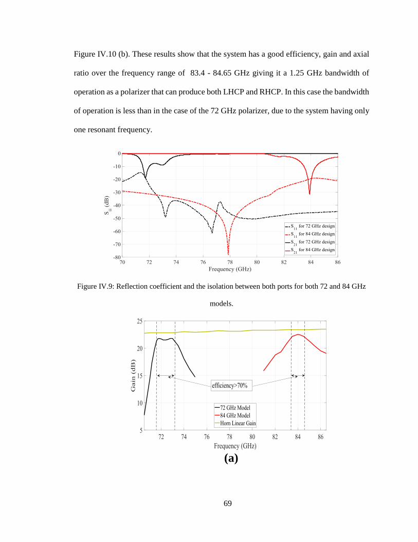
69

Figure IV.10 (b). These results show that the system has a good efficiency, gain and axial

ratio over the frequency range of 83.4 - 84.65 GHz giving it a 1.25 GHz bandwidth of

operation as a polarizer that can produce both LHCP and RHCP. In this case the bandwidth

of operation is less than in the case of the 72 GHz polarizer, due to the system having only

one resonant frequency.

Figure IV.9: Reflection coefficient and the isolation between both ports for both 72 and 84 GHz

models.

(a)

(b)

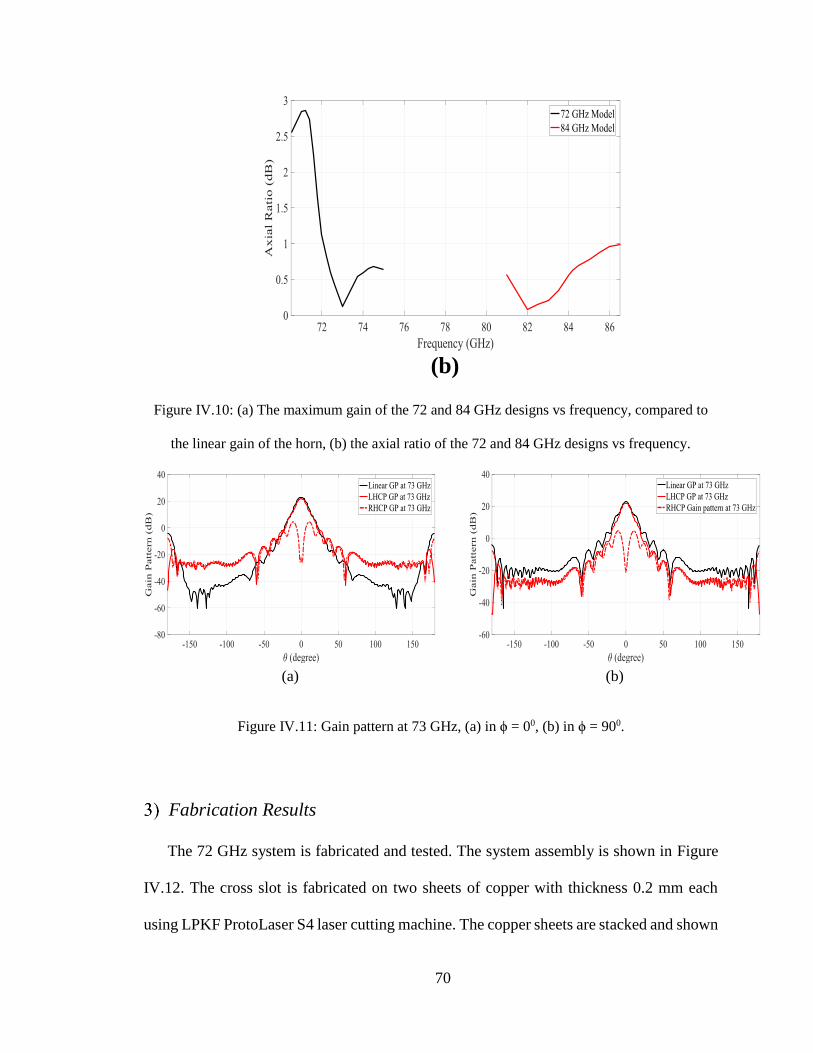
70

Figure IV.10: (a) The maximum gain of the 72 and 84 GHz designs vs frequency, compared to

the linear gain of the horn, (b) the axial ratio of the 72 and 84 GHz designs vs frequency.

Figure IV.11: Gain pattern at 73 GHz, (a) in ϕ = 00, (b) in ϕ = 900.

Fabrication Results

The 72 GHz system is fabricated and tested. The system assembly is shown in Figure

IV.12. The cross slot is fabricated on two sheets of copper with thickness 0.2 mm each

using LPKF ProtoLaser S4 laser cutting machine. The copper sheets are stacked and shown

(a)

(b)

(a) (b)

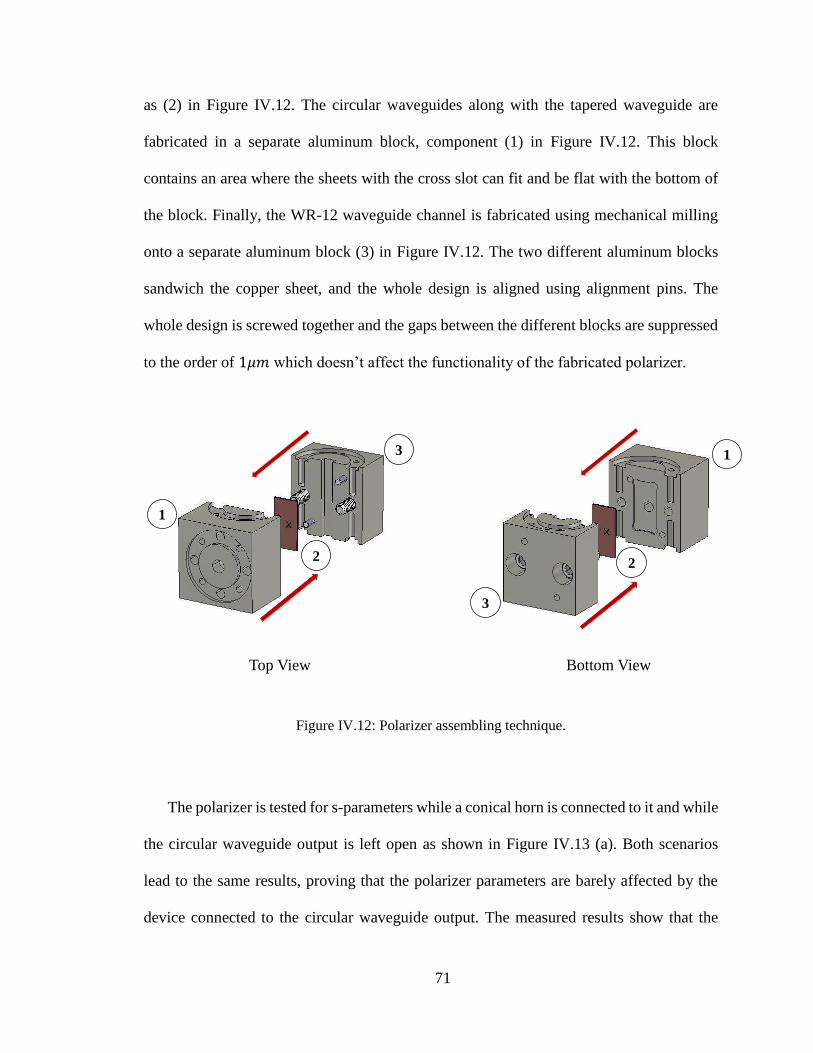
71

as (2) in Figure IV.12. The circular waveguides along with the tapered waveguide are

fabricated in a separate aluminum block, component (1) in Figure IV.12. This block

contains an area where the sheets with the cross slot can fit and be flat with the bottom of

the block. Finally, the WR-12 waveguide channel is fabricated using mechanical milling

onto a separate aluminum block (3) in Figure IV.12. The two different aluminum blocks

sandwich the copper sheet, and the whole design is aligned using alignment pins. The

whole design is screwed together and the gaps between the different blocks are suppressed

to the order of 1𝜇𝑚 which doesn’t affect the functionality of the fabricated polarizer.

Figure IV.12: Polarizer assembling technique.

The polarizer is tested for s-parameters while a conical horn is connected to it and while

the circular waveguide output is left open as shown in Figure IV.13 (a). Both scenarios

lead to the same results, proving that the polarizer parameters are barely affected by the

device connected to the circular waveguide output. The measured results show that the

Top View Bottom View

1

2

3

3

2

1

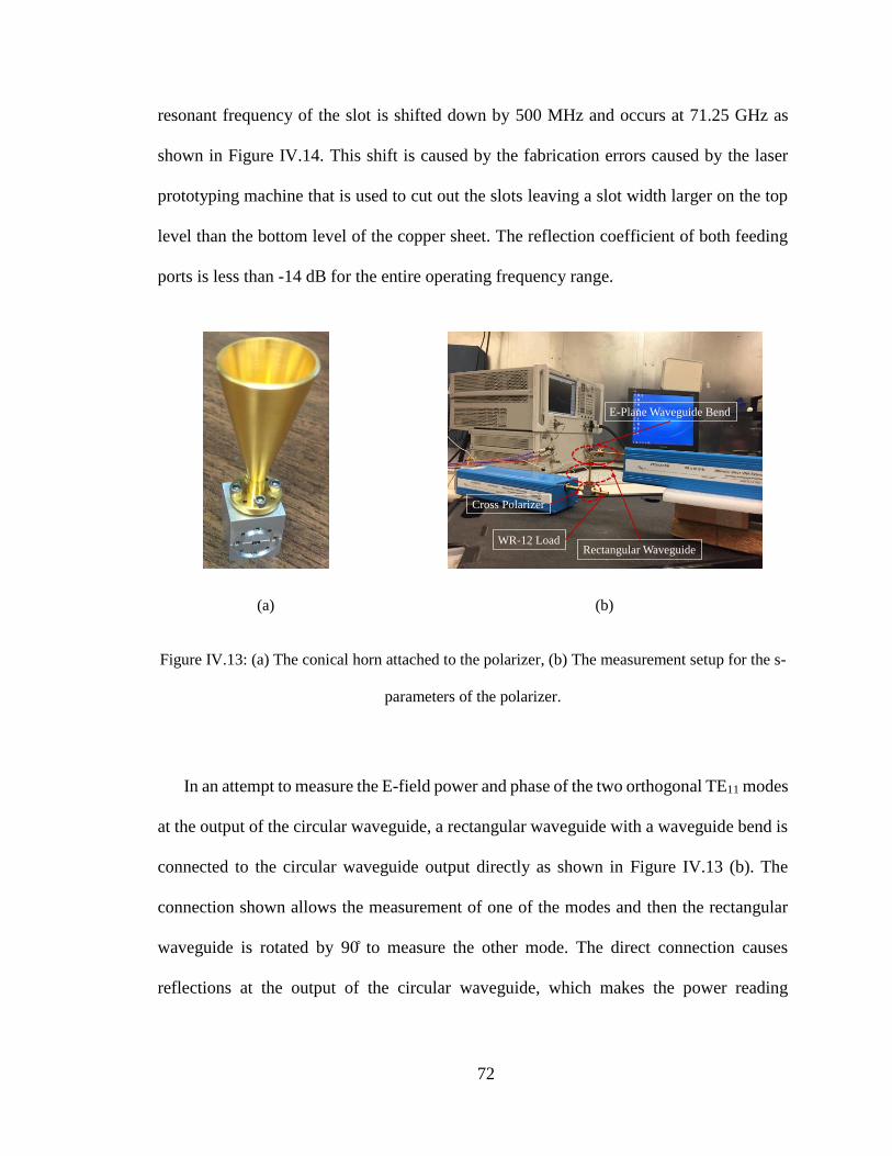
72

resonant frequency of the slot is shifted down by 500 MHz and occurs at 71.25 GHz as

shown in Figure IV.14. This shift is caused by the fabrication errors caused by the laser

prototyping machine that is used to cut out the slots leaving a slot width larger on the top

level than the bottom level of the copper sheet. The reflection coefficient of both feeding

ports is less than -14 dB for the entire operating frequency range.

Figure IV.13: (a) The conical horn attached to the polarizer, (b) The measurement setup for the s-

parameters of the polarizer.

In an attempt to measure the E-field power and phase of the two orthogonal TE11 modes

at the output of the circular waveguide, a rectangular waveguide with a waveguide bend is

connected to the circular waveguide output directly as shown in Figure IV.13 (b). The

connection shown allows the measurement of one of the modes and then the rectangular

waveguide is rotated by 90 to measure the other mode. The direct connection causes

reflections at the output of the circular waveguide, which makes the power reading

(a) (b)

Rectangular WaveguideWR-12 Load

E-Plane Waveguide Bend

Cross Polarizer

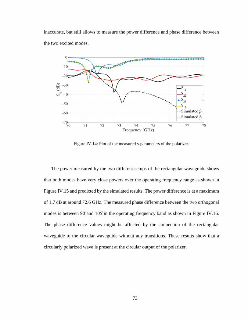
73

inaccurate, but still allows to measure the power difference and phase difference between

the two excited modes.

Figure IV.14: Plot of the measured s-parameters of the polarizer.

The power measured by the two different setups of the rectangular waveguide shows

that both modes have very close powers over the operating frequency range as shown in

Figure IV.15 and predicted by the simulated results. The power difference is at a maximum

of 1.7 dB at around 72.6 GHz. The measured phase difference between the two orthogonal

modes is between 90 and 105 in the operating frequency band as shown in Figure IV.16.

The phase difference values might be affected by the connection of the rectangular

waveguide to the circular waveguide without any transitions. These results show that a

circularly polarized wave is present at the circular output of the polarizer.

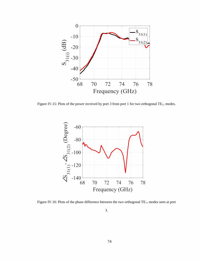
74

Figure IV.15: Plots of the power received by port 3 from port 1 for two orthogonal TE11 modes.

Figure IV.16: Plots of the phase difference between the two orthogonal TE11 modes seen at port

3.

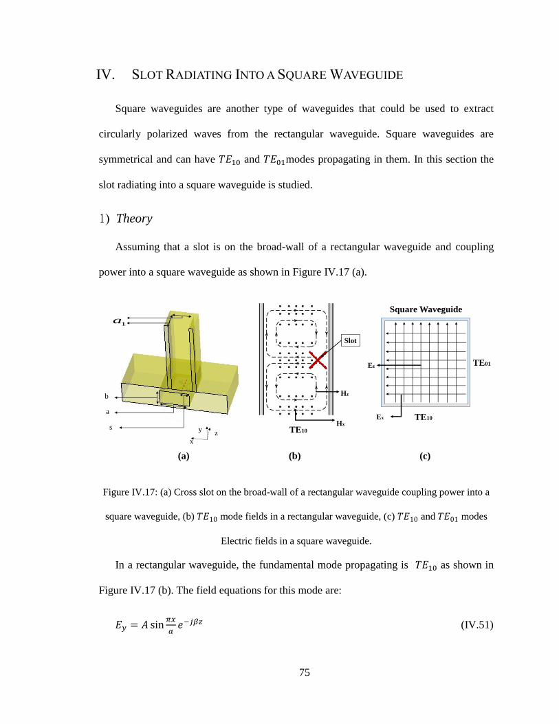
75

IV. SLOT RADIATING INTO A SQUARE WAVEGUIDE

Square waveguides are another type of waveguides that could be used to extract

circularly polarized waves from the rectangular waveguide. Square waveguides are

symmetrical and can have 𝑇𝐸10 and 𝑇𝐸01modes propagating in them. In this section the

slot radiating into a square waveguide is studied.

Theory

Assuming that a slot is on the broad-wall of a rectangular waveguide and coupling

power into a square waveguide as shown in Figure IV.17 (a).

Figure IV.17: (a) Cross slot on the broad-wall of a rectangular waveguide coupling power into a

square waveguide, (b) 𝑇𝐸10 mode fields in a rectangular waveguide, (c) 𝑇𝐸10 and 𝑇𝐸01 modes

Electric fields in a square waveguide.

In a rectangular waveguide, the fundamental mode propagating is 𝑇𝐸10 as shown in

Figure IV.17 (b). The field equations for this mode are:

𝐸 = 𝐴 sin𝜋


Hx

Hz

TE10

(b)(a)

x

yz

a

b

s

1a

Slot

TE10

TE01

Square Waveguide

(c)

Ez

Ex

76

𝐻 = −𝐴

𝑍10sin

𝜋


𝐻𝑧 = 𝑗𝜋𝐴

𝛽𝑎𝑍10cos

𝜋


where 𝑍10 = 𝑘0𝜂0

𝛽

Assuming that the slot is at a distance s from the narrow wall and at z=0, at the slot the

electric and magnetic polarizabilities are:

𝑃𝑒 = 𝐴휀0𝛼𝑒 sin𝜋

𝑎𝛿(𝑥 − 𝑠)𝛿(𝑦 − 𝑏)𝛿(𝑧) (IV.54)

𝑃𝑚 = −𝐴𝛼𝑚 [−

𝑍10sin

𝜋

𝑎+

𝑗𝜋

𝛽𝑎𝑍10cos

𝜋

𝑎] 𝛿(𝑥 − 𝑠)𝛿(𝑦 − 𝑏)𝛿(𝑧) (IV.55)

In the square waveguide, the two fundamental modes that could be excited are the 𝑇𝐸10

and the 𝑇𝐸01 modes with their electric fields are shown in Figure IV.17 (c). The fields

equations for these modes are as follows:

For 𝑇𝐸10:

𝐸 = 0 (IV.56) 𝐻 = −𝐵

𝑍10sin

𝜋( − +𝑎12)

𝑎1𝑒−𝑗𝛽1( −𝑏) (IV.57)

𝐸 = 0 (IV.58) 𝐻 = 𝑗𝜋𝐵

𝛽1𝑎1𝑍10cos

𝜋( − +𝑎12)

𝑎1𝑒−𝑗𝛽1( −𝑏) (IV.59)

𝐻𝑧 = 0 (IV.60) 𝐸𝑧 = 𝐵 sin𝜋( − +

𝑎12)

𝑎1𝑒−𝑗𝛽1( −𝑏) (IV.61)

For 𝑇𝐸01:

𝐸 = 𝐶 sin𝜋(𝑧+

𝑎12)

𝑎1𝑒−𝑗𝛽2( −𝑏) (IV.62) 𝐻 = 0 (IV.63)

77

𝐸 = 0 (IV.64) 𝐻 = 𝑗𝜋𝐶

𝛽2𝑎1𝑍01cos

𝜋(𝑧+𝑎12)

𝑎1𝑒−𝑗𝛽2( −𝑏) (IV.65)

𝐸𝑧 = 0 (IV.66) 𝐻𝑧 = −𝐶

𝑍01sin

𝜋(𝑧+𝑎12)

𝑎1𝑒−𝑗𝛽2( −𝑏) (IV.67)

B and C in the previous equations determine the magnitude and phase of the fields in

the square waveguide and their values are essential to excite a circularly polarized wave.

B and C can be expressed as two integral equations as follows:

𝐵 = −1

𝑃102∫ 𝐸10 . 𝐽 𝑣

𝑑𝑣 + 1

𝑃102∫ 𝐻10 . 𝑣

𝑑𝑣 (IV.68)

𝐶 = −1

𝑃012∫ 𝐸01 . 𝐽 𝑣

𝑑𝑣 + 1

𝑃012∫ 𝐻01 . 𝑣

𝑑𝑣 (IV.69)

Solving the integral equations leads to the following expressions of B and C:

𝐵 =1

𝑃102[ (𝑠, 𝑏, 0). 𝑃𝑒 ] =

1

𝑃102[−

1

𝑍101sin (

𝜋(𝑎12)

𝑎1) (−𝛼𝑚)𝐴(−

1

𝑍10) sin

𝜋

𝑎] =

1

𝑃102[−

𝛼𝑚𝐴

𝑍10𝑍101sin

𝜋

𝑎] (IV.70)

𝐶 =1

𝑃01[ 𝑧(𝑠, 𝑏, 0). 𝑃𝑚 ] =

1

𝑃01[1

𝑍01sin (

𝜋(𝑎12)

𝑎1) (−𝛼𝑚)𝐴(

𝑗𝜋

𝛽𝑎𝑍10) cos

𝜋

𝑎] =

−𝑗𝜋𝛼𝑚𝐴

𝑃01𝑍10𝑍01𝛽𝑎cos

𝜋

𝑎 (IV.71)

In order to have a circularly polarized wave in the square waveguide, we need the following

identities between B and C to hold true:

|𝐵| = |𝐶| and ∠𝐸𝑧10 = ∠𝐸 01 ±𝜋

2

78

if we have 𝑎 = 𝑎1 then:

𝛽 = 𝛽1 = 𝛽2

𝑍101 = 𝑍01

𝑃102 = 𝑃01

Hence, solving the magnitudes equality leads to the following:

1

𝑃102[𝛼𝑚𝐴

𝑍10𝑍101sin (

𝜋𝑠

𝑎)] =

𝜋𝛼𝑚𝐴

𝑃01𝑍10𝑍01𝛽𝑎cos (

𝜋𝑠

𝑎)

sin𝜋𝑠

𝑎=

𝜋

𝛽𝑎cos

𝜋𝑠

𝑎

tan𝜋𝑠

𝑎=

𝜋

𝛽𝑎

𝑠 =𝑎

2 ±

𝑎

𝜋tan−1√(

2 𝑎

𝑐)2 − 1 (IV.72)

Now, by examining ∠𝐸𝑧10 = ∠𝐸 01 ±𝜋

2 we notice that the ∠𝐸𝑧10 is dependent on the

∠𝐵 and the ∠𝐸 01 is dependent on the ∠𝐶. From the expressions of B and C it can be

noticed that B is a real number and C is an imaginary number, which means that:

∠𝐵 = 0 𝑎𝑛𝑑 ∠𝐶 = 𝜋

2

This means that ∠𝐵 − ∠𝐶 = −𝜋

2 hence the two electric fields in the square waveguide are

in 90° phase difference. The conditions above allow a slot in the broad-wall to radiate a

circularly polarized wave into a square waveguide. It is worth mentioning that the condition

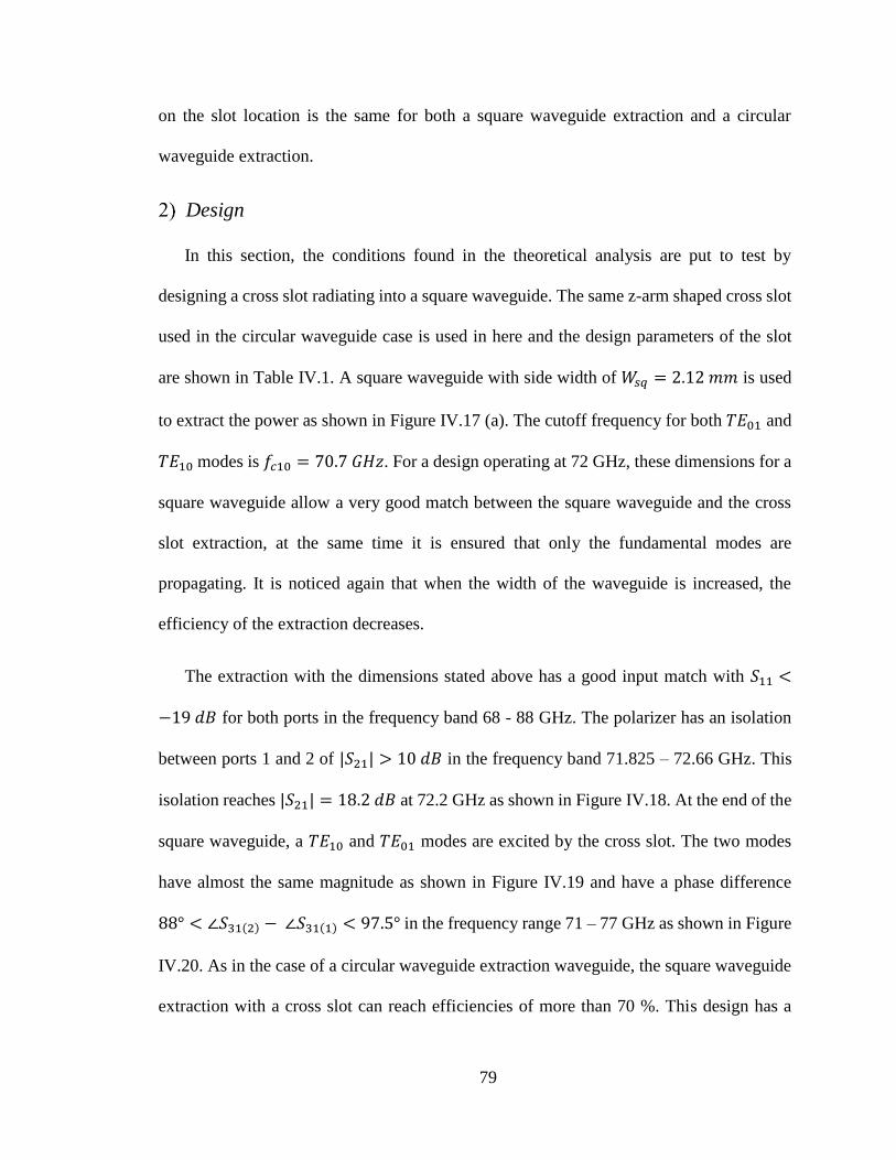
79

on the slot location is the same for both a square waveguide extraction and a circular

waveguide extraction.

Design

In this section, the conditions found in the theoretical analysis are put to test by

designing a cross slot radiating into a square waveguide. The same z-arm shaped cross slot

used in the circular waveguide case is used in here and the design parameters of the slot

are shown in Table IV.1. A square waveguide with side width of 𝑞 = 2.12 𝑚𝑚 is used

to extract the power as shown in Figure IV.17 (a). The cutoff frequency for both 𝑇𝐸01 and

𝑇𝐸10 modes is 𝑓𝑐10 = 70.7 𝐺𝐻𝑧. For a design operating at 72 GHz, these dimensions for a

square waveguide allow a very good match between the square waveguide and the cross

slot extraction, at the same time it is ensured that only the fundamental modes are

propagating. It is noticed again that when the width of the waveguide is increased, the

efficiency of the extraction decreases.

The extraction with the dimensions stated above has a good input match with 11 <

−19 𝑑𝐵 for both ports in the frequency band 68 - 88 GHz. The polarizer has an isolation

between ports 1 and 2 of | 21| > 10 𝑑𝐵 in the frequency band 71.825 – 72.66 GHz. This

isolation reaches | 21| = 18.2 𝑑𝐵 at 72.2 GHz as shown in Figure IV.18. At the end of the

square waveguide, a 𝑇𝐸10 and 𝑇𝐸01 modes are excited by the cross slot. The two modes

have almost the same magnitude as shown in Figure IV.19 and have a phase difference

88° < ∠ 31(2) − ∠ 31(1) < 97.5° in the frequency range 71 – 77 GHz as shown in Figure

IV.20. As in the case of a circular waveguide extraction waveguide, the square waveguide

extraction with a cross slot can reach efficiencies of more than 70 %. This design has a

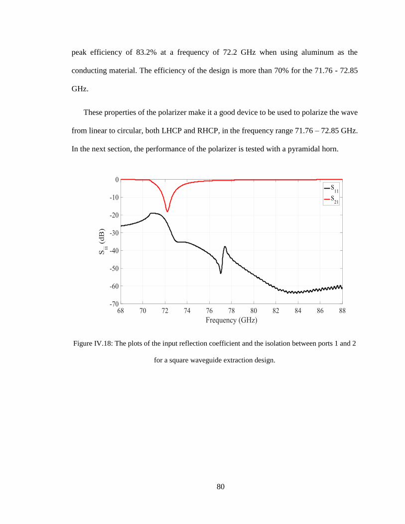
80

peak efficiency of 83.2% at a frequency of 72.2 GHz when using aluminum as the

conducting material. The efficiency of the design is more than 70% for the 71.76 - 72.85

GHz.

These properties of the polarizer make it a good device to be used to polarize the wave

from linear to circular, both LHCP and RHCP, in the frequency range 71.76 – 72.85 GHz.

In the next section, the performance of the polarizer is tested with a pyramidal horn.

Figure IV.18: The plots of the input reflection coefficient and the isolation between ports 1 and 2

for a square waveguide extraction design.

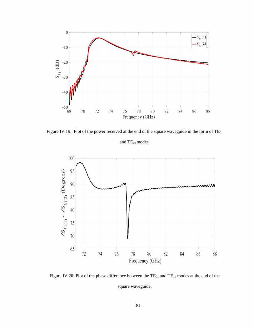
81

Figure IV.19: Plot of the power received at the end of the square waveguide in the form of TE01

and TE10 modes.

Figure IV.20: Plot of the phase difference between the TE01 and TE10 modes at the end of the

square waveguide.

82

V. A SINGLE SLOT FEEDING A PYRAMIDAL HORN ANTENNA

For this section, the polarizer designed in section IV is tested by feeding a pyramidal

horn antenna.

Horn Antenna Design

For the applications targeted by this dissertation, the pyramidal horn should have a high

gain and yield circular polarization. For the circular polarization to be able to propagate,

the pyramidal horn should have both identical E and H planes.

In order to achieve a maximum stable gain of around 23 dB, the iterative process

described in [61] is used. The iterative process holds the following equality true:

(√2𝜒 −𝑏

𝜆)2(2𝜒 − 1) = (

𝐺0

2𝜋√

3

2𝜋

1

√𝜒−

𝑎

𝜆)

2

(𝐺0

6𝜋31

𝜒− 1) (IV.73)

Where 𝜒 = 𝜌𝑒/𝜆 and 𝜌ℎ

𝜆=

𝐺02

8𝜋31

𝜒, and a, b, 𝜌𝑒𝑎𝑛𝑑 𝜌 are defined in Figure IV.21 and

𝐺0 is the dimensionless gain of the antenna.

Once the correct value of 𝜒 is found, all the other parameters of the design can be found.

In this case, we have = 𝑏 , 𝑎1 = 𝑏1 and 𝜌𝑒 = 𝜌 . The dimensions of the pyramidal horn

that lead to a gain of around 23 dB are stated in Table IV.3. For the horn to have a good

match with the polarizer, a square waveguide with 𝑎 = 𝑏 = 2.12 𝑚𝑚 is used to feed it.

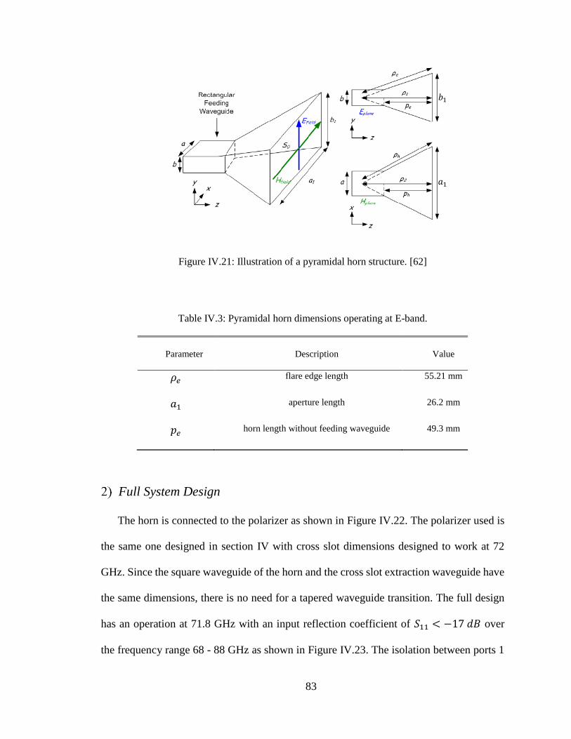
83

Figure IV.21: Illustration of a pyramidal horn structure. [62]

Table IV.3: Pyramidal horn dimensions operating at E-band.


𝜌𝑒 flare edge length 55.21 mm

𝑎1 aperture length 26.2 mm

𝑝𝑒 horn length without feeding waveguide 49.3 mm

Full System Design

The horn is connected to the polarizer as shown in Figure IV.22. The polarizer used is

the same one designed in section IV with cross slot dimensions designed to work at 72

GHz. Since the square waveguide of the horn and the cross slot extraction waveguide have

the same dimensions, there is no need for a tapered waveguide transition. The full design

has an operation at 71.8 GHz with an input reflection coefficient of 11 < −17 𝑑𝐵 over

the frequency range 68 - 88 GHz as shown in Figure IV.23. The isolation between ports 1

𝑏1

𝑎1

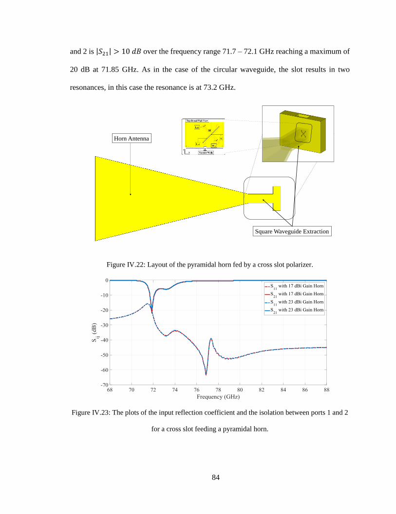
84

and 2 is | 21| > 10 𝑑𝐵 over the frequency range 71.7 – 72.1 GHz reaching a maximum of

20 dB at 71.85 GHz. As in the case of the circular waveguide, the slot results in two

resonances, in this case the resonance is at 73.2 GHz.

Figure IV.22: Layout of the pyramidal horn fed by a cross slot polarizer.

Figure IV.23: The plots of the input reflection coefficient and the isolation between ports 1 and 2

for a cross slot feeding a pyramidal horn.

Horn Antenna

Square Waveguide Extraction

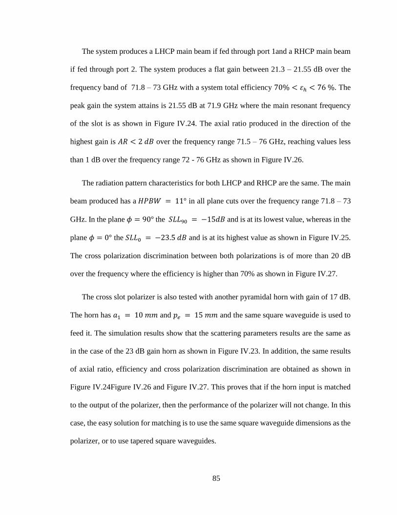
85

The system produces a LHCP main beam if fed through port 1and a RHCP main beam

if fed through port 2. The system produces a flat gain between 21.3 – 21.55 dB over the

frequency band of 71.8 – 73 GHz with a system total efficiency 70% < 휀 < 76 %. The

peak gain the system attains is 21.55 dB at 71.9 GHz where the main resonant frequency

of the slot is as shown in Figure IV.24. The axial ratio produced in the direction of the

highest gain is 𝐴 < 2 𝑑𝐵 over the frequency range 71.5 – 76 GHz, reaching values less

than 1 dB over the frequency range 72 - 76 GHz as shown in Figure IV.26.

The radiation pattern characteristics for both LHCP and RHCP are the same. The main

beam produced has a 𝐻𝑃𝐵 = 11° in all plane cuts over the frequency range 71.8 – 73

GHz. In the plane 𝜙 = 90° the 90 = −15𝑑𝐵 and is at its lowest value, whereas in the

plane 𝜙 = 0° the 0 = −23.5 𝑑𝐵 and is at its highest value as shown in Figure IV.25.

The cross polarization discrimination between both polarizations is of more than 20 dB

over the frequency where the efficiency is higher than 70% as shown in Figure IV.27.

The cross slot polarizer is also tested with another pyramidal horn with gain of 17 dB.

The horn has 𝑎1 = 10 𝑚𝑚 and 𝑝𝑒 = 15 𝑚𝑚 and the same square waveguide is used to

feed it. The simulation results show that the scattering parameters results are the same as

in the case of the 23 dB gain horn as shown in Figure IV.23. In addition, the same results

of axial ratio, efficiency and cross polarization discrimination are obtained as shown in

Figure IV.24Figure IV.26 and Figure IV.27. This proves that if the horn input is matched

to the output of the polarizer, then the performance of the polarizer will not change. In this

case, the easy solution for matching is to use the same square waveguide dimensions as the

polarizer, or to use tapered square waveguides.

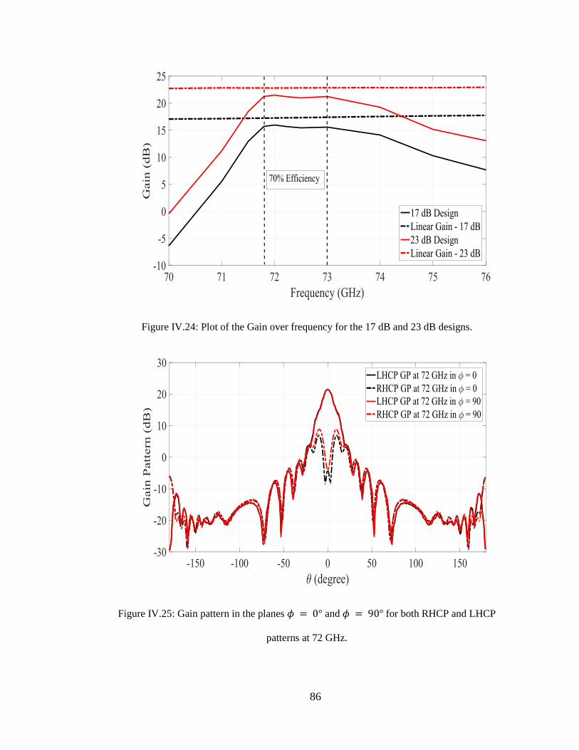
86

Figure IV.24: Plot of the Gain over frequency for the 17 dB and 23 dB designs.

Figure IV.25: Gain pattern in the planes 𝜙 = 0° and 𝜙 = 90° for both RHCP and LHCP

patterns at 72 GHz.

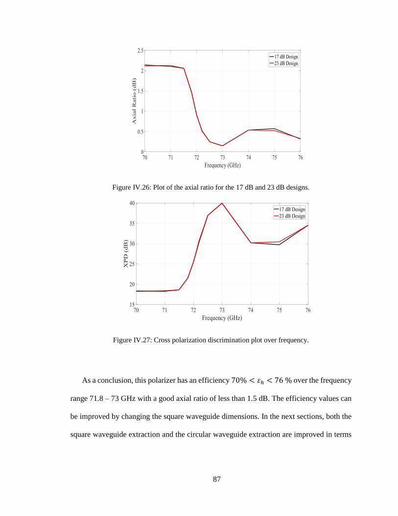
87

Figure IV.26: Plot of the axial ratio for the 17 dB and 23 dB designs.

Figure IV.27: Cross polarization discrimination plot over frequency.

As a conclusion, this polarizer has an efficiency 70% < 휀 < 76 % over the frequency

range 71.8 – 73 GHz with a good axial ratio of less than 1.5 dB. The efficiency values can

be improved by changing the square waveguide dimensions. In the next sections, both the

square waveguide extraction and the circular waveguide extraction are improved in terms

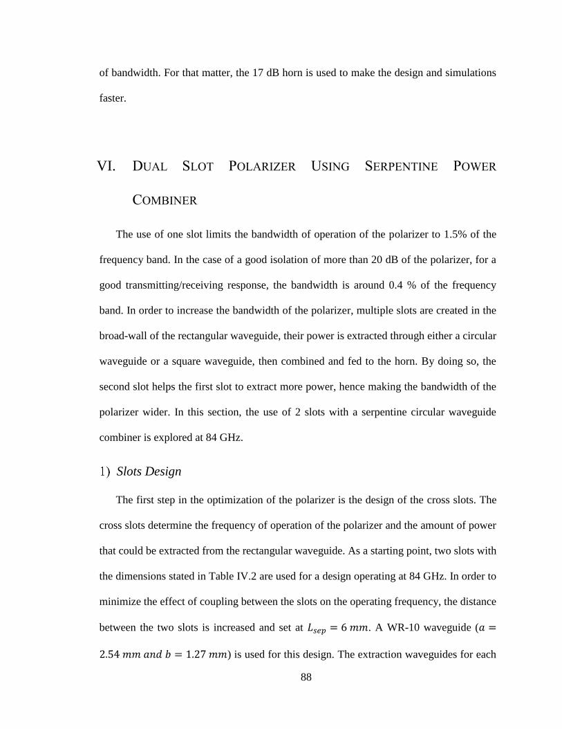
88

of bandwidth. For that matter, the 17 dB horn is used to make the design and simulations

faster.

VI. DUAL SLOT POLARIZER USING SERPENTINE POWER

COMBINER

The use of one slot limits the bandwidth of operation of the polarizer to 1.5% of the

frequency band. In the case of a good isolation of more than 20 dB of the polarizer, for a

good transmitting/receiving response, the bandwidth is around 0.4 % of the frequency

band. In order to increase the bandwidth of the polarizer, multiple slots are created in the

broad-wall of the rectangular waveguide, their power is extracted through either a circular

waveguide or a square waveguide, then combined and fed to the horn. By doing so, the

second slot helps the first slot to extract more power, hence making the bandwidth of the

polarizer wider. In this section, the use of 2 slots with a serpentine circular waveguide

combiner is explored at 84 GHz.

Slots Design

The first step in the optimization of the polarizer is the design of the cross slots. The

cross slots determine the frequency of operation of the polarizer and the amount of power

that could be extracted from the rectangular waveguide. As a starting point, two slots with

the dimensions stated in Table IV.2 are used for a design operating at 84 GHz. In order to

minimize the effect of coupling between the slots on the operating frequency, the distance

between the two slots is increased and set at 𝑒𝑝 = 6 𝑚𝑚. A WR-10 waveguide (𝑎 =

2.54 𝑚𝑚 𝑎𝑛𝑑 𝑏 = 1.27 𝑚𝑚) is used for this design. The extraction waveguides for each

89

slot have a cross section diameter of 𝑒 = 2.5 𝑚𝑚 and a length minimized to 𝑒 =

5 𝑚𝑚. When adding the extraction waveguides a mismatch between the slots and the

waveguides takes place. This mismatch can be solved by changing the dimensions of the

slots in order to extract the maximum power from the rectangular waveguide. In addition,

when the extraction waveguides are connected using the serpentine power combiner, more

loading is added on the slots, which changes their operating frequency and efficiency. The

final slots dimensions are shown in Table IV.4.

Another configuration of the slots, that could increase the bandwidth of operation, is

by having the resonant frequencies of the slots close to each other, but not the same. This

configuration is studied in the section of square waveguides combiners.

Table IV.4: Dimensions of the Z-shaped arm cross-slots at 84 GHz used in the serpentine power

combiner.






𝛼2 arm angle with y-axis 43°


90

Serpentine Power Combiner Design

In order to combine the power extracted by the two cross slots, a serpentine power

combiner is used. The serpentine power combiner has two circular waveguide inputs and

one circular waveguide output. Each section of the input waveguides has a convex

curvature followed by a concave curvature or vice versa as shown in Figure IV.28 (a).

These curvatures are arcs of a circle connected smoothly. These two sections intersect at

the output waveguide. The radius of all waveguides used in the serpentine design is

optimized to be 𝑤 = 1.25 𝑚𝑚 with a cutoff frequency 𝑓𝑐 = 70.33 𝐺𝐻𝑧 for the

fundamental mode 𝑇𝐸11 and a cutoff frequency for 𝑇𝑀01, 𝑓𝑐 = 91.9 𝐺𝐻𝑧, ensuring that

only the fundamental mode is traveling inside the waveguide at 84 GHz.

The curvatures of the serpentine waveguides have a radius 𝑒 𝑝 = 45 𝑚𝑚 as shown

in Figure IV.28 (b). The curvature radius ensures that at the intersection plane of the two

sections of the serpentine, the geometry is smooth with respect to the operating wavelength.

The smoothness ensures that the wave is not scattered when it hits the intersection plane

and the phase of each 𝑇𝐸11 mode is preserved. This ensures that the 90° phase difference

is intact and the orthogonal components of the electric field have close magnitudes.

The separation between the slots along with 𝑒 𝑝, shown in Figure IV.28 (b), are

chosen in a way that makes each section of the serpentine input waveguides well matched

with the serpentine output waveguide. If this matching is not done correctly, a standing

wave is seen in the section of the waveguide that extracts the least power, causing the

efficiency of the combiner to drop. In this design, the separation between the slots is

optimized to be = 10 𝑚𝑚 for 𝑒 𝑝 = 45 𝑚𝑚. All these factors are essential in

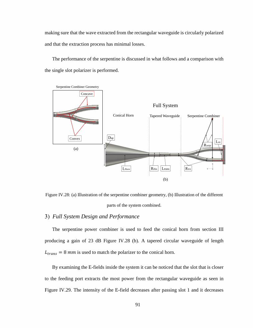
91

making sure that the wave extracted from the rectangular waveguide is circularly polarized

and that the extraction process has minimal losses.

The performance of the serpentine is discussed in what follows and a comparison with

the single slot polarizer is performed.

Figure IV.28: (a) Illustration of the serpentine combiner geometry, (b) Illustration of the different

parts of the system combined.

Full System Design and Performance

The serpentine power combiner is used to feed the conical horn from section III

producing a gain of 23 dB Figure IV.28 (b). A tapered circular waveguide of length

𝑎𝑛 = 8 𝑚𝑚 is used to match the polarizer to the conical horn.

By examining the E-fields inside the system it can be noticed that the slot that is closer

to the feeding port extracts the most power from the rectangular waveguide as seen in

Figure IV.29. The intensity of the E-field decreases after passing slot 1 and it decreases

RHin Rws

Rserp

Ltrans

Lss

Conical Horn Tapered Waveguide Serpentine Combiner

LHorn

Dap

Serpentine Combiner Geometry

Concave

Convex

(a)

(b)

Full System

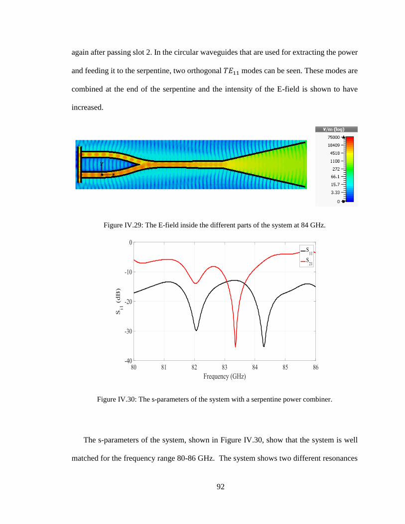
92

again after passing slot 2. In the circular waveguides that are used for extracting the power

and feeding it to the serpentine, two orthogonal 𝑇𝐸11 modes can be seen. These modes are

combined at the end of the serpentine and the intensity of the E-field is shown to have

increased.

Figure IV.29: The E-field inside the different parts of the system at 84 GHz.

Figure IV.30: The s-parameters of the system with a serpentine power combiner.

The s-parameters of the system, shown in Figure IV.30, show that the system is well

matched for the frequency range 80-86 GHz. The system shows two different resonances

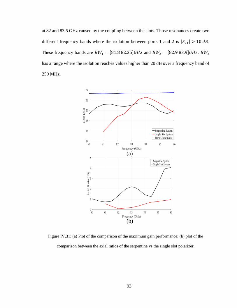
93

at 82 and 83.5 GHz caused by the coupling between the slots. Those resonances create two

different frequency bands where the isolation between ports 1 and 2 is | 21| > 10 𝑑𝐵.

These frequency bands are 𝐵 1 = [81.8 82.35]𝐺𝐻𝑧 and 𝐵 2 = [82.9 83.9]𝐺𝐻𝑧. 𝐵 2

has a range where the isolation reaches values higher than 20 dB over a frequency band of

250 MHz.

Figure IV.31: (a) Plot of the comparison of the maximum gain performance; (b) plot of the

comparison between the axial ratios of the serpentine vs the single slot polarizer.

(a)

(b)

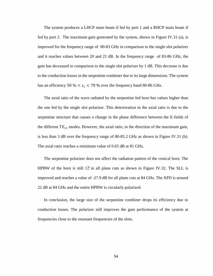
94

The system produces a LHCP main beam if fed by port 1 and a RHCP main beam if

fed by port 2. The maximum gain generated by the system, shown in Figure IV.31 (a), is

improved for the frequency range of 80-83 GHz in comparison to the single slot polarizer

and it reaches values between 20 and 21 dB. In the frequency range of 83-86 GHz, the

gain has decreased in comparison to the single slot polarizer by 1 dB. This decrease is due

to the conduction losses in the serpentine combiner due to its large dimensions. The system

has an efficiency 50 % < 휀 < 70 % over the frequency band 80-86 GHz.

The axial ratio of the wave radiated by the serpentine fed horn has values higher than

the one fed by the single slot polarizer. This deterioration in the axial ratio is due to the

serpentine structure that causes a change in the phase difference between the E-fields of

the different 𝑇𝐸11 modes. However, the axial ratio, in the direction of the maximum gain,

is less than 3 dB over the frequency range of 80-85.2 GHz as shown in Figure IV.31 (b).

The axial ratio reaches a minimum value of 0.65 dB at 81 GHz.

The serpentine polarizer does not affect the radiation pattern of the conical horn. The

HPBW of the horn is still 12 in all plane cuts as shown in Figure IV.32. The SLL is

improved and reaches a value of -27.9 dB for all plane cuts at 84 GHz. The XPD is around

22 dB at 84 GHz and the entire HPBW is circularly polarized.

In conclusion, the large size of the serpentine combiner drops its efficiency due to

conduction losses. The polarizer still improves the gain performance of the system at

frequencies close to the resonant frequencies of the slots.

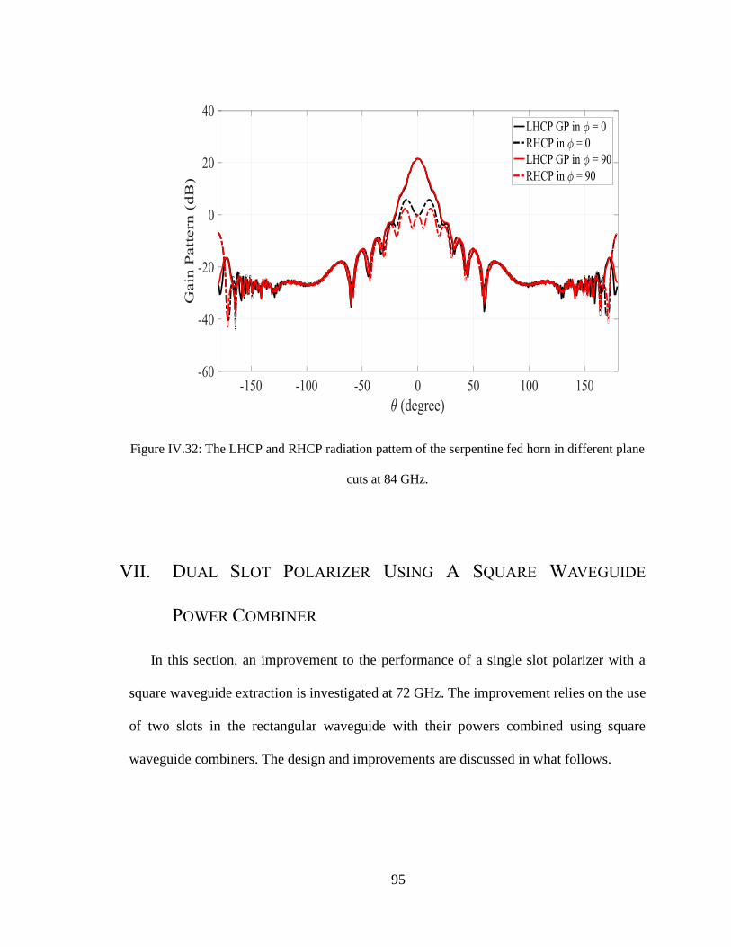
95

Figure IV.32: The LHCP and RHCP radiation pattern of the serpentine fed horn in different plane

cuts at 84 GHz.

VII. DUAL SLOT POLARIZER USING A SQUARE WAVEGUIDE

POWER COMBINER

In this section, an improvement to the performance of a single slot polarizer with a

square waveguide extraction is investigated at 72 GHz. The improvement relies on the use

of two slots in the rectangular waveguide with their powers combined using square

waveguide combiners. The design and improvements are discussed in what follows.

96

Dual Slot Design

Same as in the case of the serpentine combiner, the first step in designing this system

is the design of the cross slots. By determining the right configuration of the slots, the

bandwidth and efficiency of the system can be improved. Two different scenarios are

considered for this matter and explained below:

Scenario 1. The slots have the same resonant frequency:

For this scenario, the slots used have the same exact dimensions which lead to the same

resonant frequency. The aim of this design is to increase the isolation between ports 1 and

2 to very high values and to have the best axial ratio values between the different

components of the electric field. The slots used in this design have their dimensions stated

in Table IV.5.

Scenario 2. The slots have close resonance frequencies

In this scenario, the slots used have dimensions that are different but very close. This

configuration of the slots results in a wider bandwidth of operation of the polarizer and in

higher efficiencies of the system over a wider frequency range than in scenario 1. The

dimensions of the slots are state in Table IV.5.

The slots are located on the broad-wall of a WR-12 waveguide and have a separation

distance of = 6 𝑚𝑚 for both scenarios. For both scenarios, the frequency of operation

is close to 72 GHz. The coupling between the slots along with the dimensions of the slots

contributed to the frequency shift between the different designs.

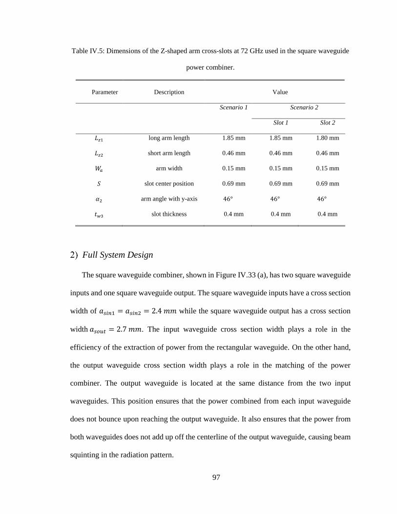
97

Table IV.5: Dimensions of the Z-shaped arm cross-slots at 72 GHz used in the square waveguide

power combiner.


Scenario 1 Scenario 2

Slot 1 Slot 2

𝑧1 long arm length 1.85 mm 1.85 mm 1.80 mm

𝑧2 short arm length 0.46 mm 0.46 mm 0.46 mm

𝑎 arm width 0.15 mm 0.15 mm 0.15 mm

slot center position 0.69 mm 0.69 mm 0.69 mm

𝛼2 arm angle with y-axis 46° 46° 46°

𝑡𝑤3 slot thickness 0.4 mm 0.4 mm 0.4 mm

Full System Design

The square waveguide combiner, shown in Figure IV.33 (a), has two square waveguide

inputs and one square waveguide output. The square waveguide inputs have a cross section

width of 𝑎 𝑖𝑛1 = 𝑎 𝑖𝑛2 = 2.4 𝑚𝑚 while the square waveguide output has a cross section

width 𝑎 𝑢 = 2.7 𝑚𝑚. The input waveguide cross section width plays a role in the

efficiency of the extraction of power from the rectangular waveguide. On the other hand,

the output waveguide cross section width plays a role in the matching of the power

combiner. The output waveguide is located at the same distance from the two input

waveguides. This position ensures that the power combined from each input waveguide

does not bounce upon reaching the output waveguide. It also ensures that the power from

both waveguides does not add up off the centerline of the output waveguide, causing beam

squinting in the radiation pattern.

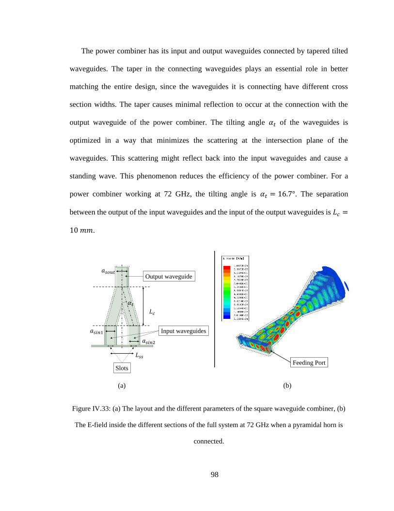
98

The power combiner has its input and output waveguides connected by tapered tilted

waveguides. The taper in the connecting waveguides plays an essential role in better

matching the entire design, since the waveguides it is connecting have different cross

section widths. The taper causes minimal reflection to occur at the connection with the

output waveguide of the power combiner. The tilting angle 𝛼 of the waveguides is

optimized in a way that minimizes the scattering at the intersection plane of the

waveguides. This scattering might reflect back into the input waveguides and cause a

standing wave. This phenomenon reduces the efficiency of the power combiner. For a

power combiner working at 72 GHz, the tilting angle is 𝛼 = 16.7°. The separation

between the output of the input waveguides and the input of the output waveguides is 𝑐 =

10 𝑚𝑚.

Figure IV.33: (a) The layout and the different parameters of the square waveguide combiner, (b)

The E-field inside the different sections of the full system at 72 GHz when a pyramidal horn is

connected.

Slots

Input waveguides

Output waveguide

𝛼 𝑐

𝑎 𝑢

𝑎 𝑖𝑛1

𝑎 𝑖𝑛2

(a) (b)

Feeding Port

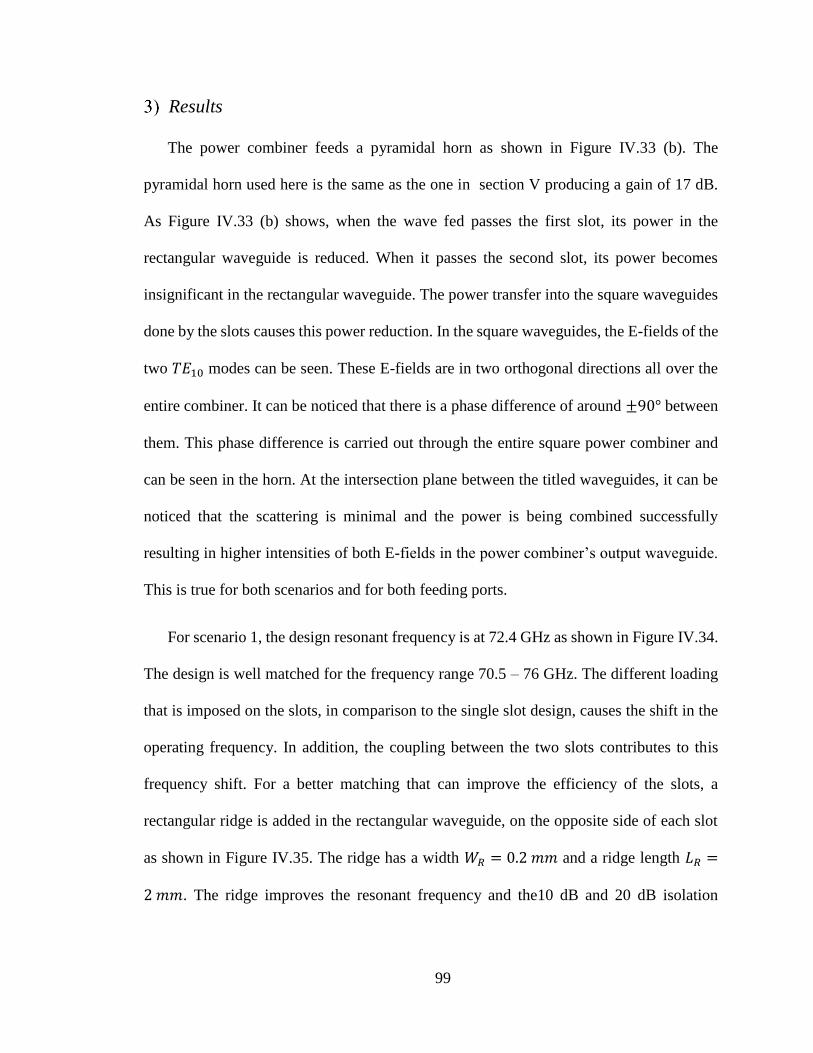
99

Results

The power combiner feeds a pyramidal horn as shown in Figure IV.33 (b). The

pyramidal horn used here is the same as the one in section V producing a gain of 17 dB.

As Figure IV.33 (b) shows, when the wave fed passes the first slot, its power in the

rectangular waveguide is reduced. When it passes the second slot, its power becomes

insignificant in the rectangular waveguide. The power transfer into the square waveguides

done by the slots causes this power reduction. In the square waveguides, the E-fields of the

two 𝑇𝐸10 modes can be seen. These E-fields are in two orthogonal directions all over the

entire combiner. It can be noticed that there is a phase difference of around ±90° between

them. This phase difference is carried out through the entire square power combiner and

can be seen in the horn. At the intersection plane between the titled waveguides, it can be

noticed that the scattering is minimal and the power is being combined successfully

resulting in higher intensities of both E-fields in the power combiner’s output waveguide.

This is true for both scenarios and for both feeding ports.

For scenario 1, the design resonant frequency is at 72.4 GHz as shown in Figure IV.34.

The design is well matched for the frequency range 70.5 – 76 GHz. The different loading

that is imposed on the slots, in comparison to the single slot design, causes the shift in the

operating frequency. In addition, the coupling between the two slots contributes to this

frequency shift. For a better matching that can improve the efficiency of the slots, a

rectangular ridge is added in the rectangular waveguide, on the opposite side of each slot

as shown in Figure IV.35. The ridge has a width 𝑅 = 0.2 𝑚𝑚 and a ridge length 𝑅 =

2 𝑚𝑚. The ridge improves the resonant frequency and the10 dB and 20 dB isolation

100

between ports 1 and 2 as shown in Figure IV.34, along with the efficiency of the system.

The ridge does not affect the input matching bandwidth.

Figure IV.34: S-parameters comparison between a regular combiner and a combiner with a ridge.

Figure IV.35: Illustration of the design with and without a ridge in the rectangular waveguide.

Without Ridge

With Ridge

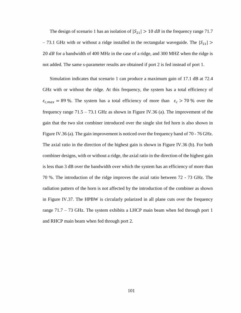
101

The design of scenario 1 has an isolation of | 21| > 10 𝑑𝐵 in the frequency range 71.7

– 73.1 GHz with or without a ridge installed in the rectangular waveguide. The | 21| >

20 𝑑𝐵 for a bandwidth of 400 MHz in the case of a ridge, and 300 MHZ when the ridge is

not added. The same s-parameter results are obtained if port 2 is fed instead of port 1.

Simulation indicates that scenario 1 can produce a maximum gain of 17.1 dB at 72.4

GHz with or without the ridge. At this frequency, the system has a total efficiency of

휀𝑐,𝑚𝑎 = 89 %. The system has a total efficiency of more than 휀𝑐 > 70 % over the

frequency range 71.5 – 73.1 GHz as shown in Figure IV.36 (a). The improvement of the

gain that the two slot combiner introduced over the single slot fed horn is also shown in

Figure IV.36 (a). The gain improvement is noticed over the frequency band of 70 - 76 GHz.

The axial ratio in the direction of the highest gain is shown in Figure IV.36 (b). For both

combiner designs, with or without a ridge, the axial ratio in the direction of the highest gain

is less than 3 dB over the bandwidth over which the system has an efficiency of more than

70 %. The introduction of the ridge improves the axial ratio between 72 - 73 GHz. The

radiation pattern of the horn is not affected by the introduction of the combiner as shown

in Figure IV.37. The HPBW is circularly polarized in all plane cuts over the frequency

range 71.7 – 73 GHz. The system exhibits a LHCP main beam when fed through port 1

and RHCP main beam when fed through port 2.

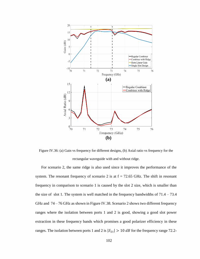
102

Figure IV.36: (a) Gain vs frequency for different designs, (b) Axial ratio vs frequency for the

rectangular waveguide with and without ridge.

For scenario 2, the same ridge is also used since it improves the performance of the

system. The resonant frequency of scenario 2 is at f = 72.65 GHz. The shift in resonant

frequency in comparison to scenario 1 is caused by the slot 2 size, which is smaller than

the size of slot 1. The system is well matched in the frequency bandwidths of 71.4 – 73.4

GHz and 74 – 76 GHz as shown in Figure IV.38. Scenario 2 shows two different frequency

ranges where the isolation between ports 1 and 2 is good, showing a good slot power

extraction in these frequency bands which promises a good polarizer efficiency in these

ranges. The isolation between ports 1 and 2 is | 21| > 10 𝑑𝐵 for the frequency range 72.2-

(a)

(b)

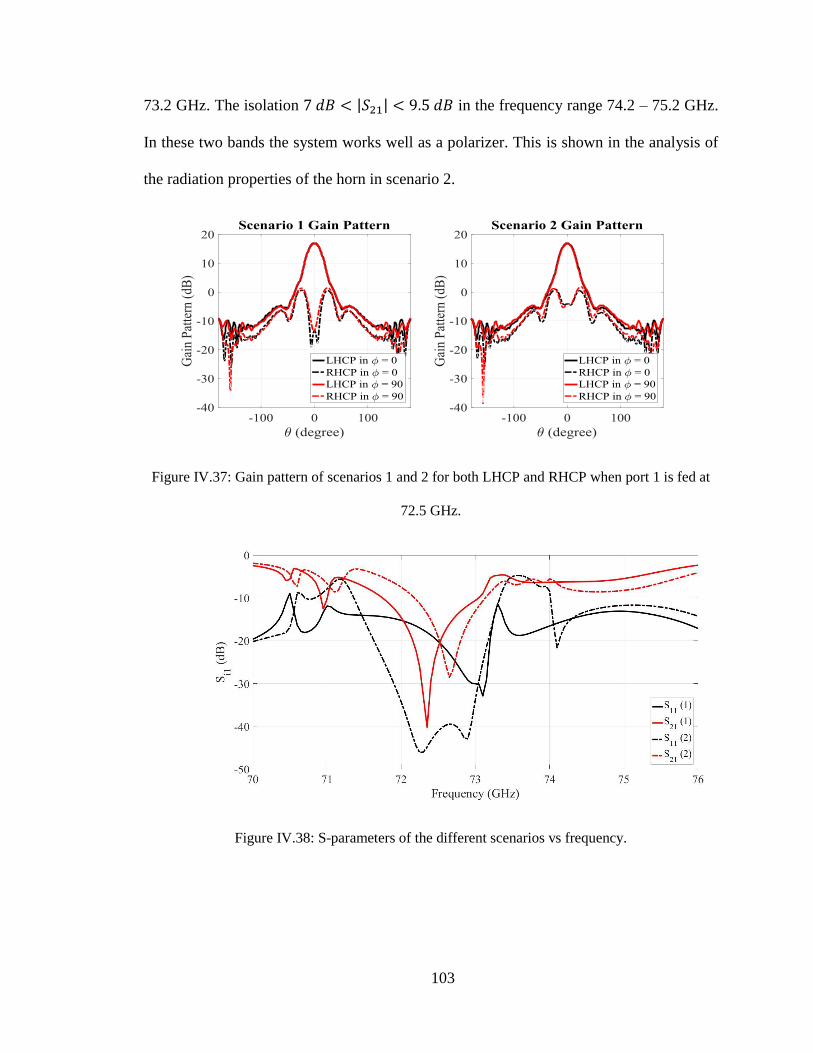
103

73.2 GHz. The isolation 7 𝑑𝐵 < | 21| < 9.5 𝑑𝐵 in the frequency range 74.2 – 75.2 GHz.

In these two bands the system works well as a polarizer. This is shown in the analysis of

the radiation properties of the horn in scenario 2.

Figure IV.37: Gain pattern of scenarios 1 and 2 for both LHCP and RHCP when port 1 is fed at

72.5 GHz.

Figure IV.38: S-parameters of the different scenarios vs frequency.

104

The maximum gain achieved in scenario 2 is 17.1 dB at 71.65 GHz. The system total

efficiency is 휀𝑐,𝑚𝑎 = 84 % at this frequency. This scenario exhibits two frequency ranges,

𝐵 1 = [71.9 73.1] 𝐺𝐻𝑧 and 𝐵 2 = [74.3 75.2] 𝐺𝐻𝑧 where the system total efficiency

is 휀𝑐 > 70 % as shown in Figure IV.39 (a). The axial ratio over these two frequency

bandwidths is less than 3 dB as shown in Figure IV.39 (b). It can be noticed that over 𝐵 1,

the axial ratio of scenario 2 is higher than scenario 1. This deterioration in axial ratio is

caused by slot 2 since it has a resonance at a higher frequency (Section IV shows that the

axial ratio is higher before the resonant frequency of the slot). In 𝐵 2, both the gain and

the axial ratio of scenario 2 are improved in comparison to scenario 1. The radiation pattern

of the horn is not affected by scenario 2 as shown in Figure IV.37. The SLL and HPBW

are the same as in the case of a linear gain horn. The HPBW of the system is entirely

circularly polarized, exhibiting a LHCP when fed through port 1 and a RHCP when fed

through port 2 and an axial ratio 𝐴 > 3 𝑑𝐵 for all the angles and the plane cuts.

As a conclusion, scenario 1 improves the bandwidth over which the system has a good

efficiency and a good isolation between both ports. The system works as an efficient

polarizer for a bandwidth of 2.2 % of the frequency band. Scenario 2 creates two separated,

but close frequency bands where the system works well as a polarizer with a bandwidth of

1.4 and 1.6 % of the frequency band.

The property illustrated in scenario 2 is further investigated in the following section in

order to create a system that can work at frequency bands that are far apart from each other

and where no single OMT polarizer can cover them.

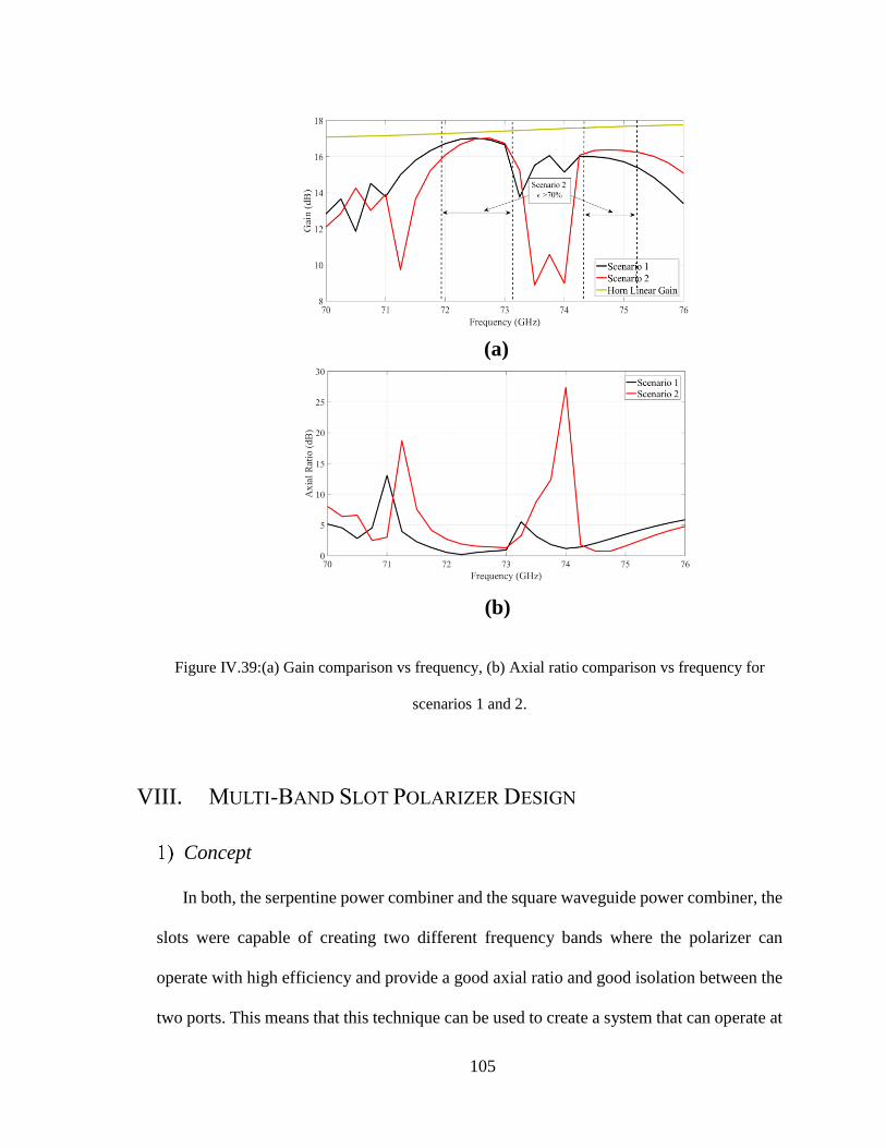
105

Figure IV.39:(a) Gain comparison vs frequency, (b) Axial ratio comparison vs frequency for

scenarios 1 and 2.

VIII. MULTI-BAND SLOT POLARIZER DESIGN

Concept

In both, the serpentine power combiner and the square waveguide power combiner, the

slots were capable of creating two different frequency bands where the polarizer can

operate with high efficiency and provide a good axial ratio and good isolation between the

two ports. This means that this technique can be used to create a system that can operate at

(a)

(b)

106

two frequency bands that are far away from each other and still provide the desired antenna

properties . The large frequency gap between the slots that are used, removes the effect of

coupling on the slots. Since the emphasis of this dissertation is on the wave propagation

at 72 and 84 GHz, a system that operates at these two frequencies is designed using several

scenarios for the design.

Dual Horn Design

The first way of realizing such system is by using a slot that works at 72 GHz and

another one that works at 84 GHz. The slots will have minimum coupling between them

since they have resonances at frequencies that are far away from each other. The slot

dimensions are indicated in Table IV.6. The slots feed two circular waveguides of radii

72 = 2.5 𝑚𝑚 𝑎𝑛𝑑 84 = 2.2 𝑚𝑚, that in turn feed two different horns as shown in

Figure IV.40. Tapered waveguides are used to connect the circular waveguides to the input

of each horn. The tapered waveguide of the 72 GHz slot has a length of 𝑎𝑛 72 = 3 𝑚𝑚

while the one for the 84 GHz slot has a length of 𝑎𝑛 84 = 8 𝑚𝑚. The 72 GHz slot is on

the broad-wall of a WR-12 waveguide while the 84 GHz slot is on the broad-wall of a WR-

10 waveguide. The two rectangular waveguides are connected by tapered waveguides and

the feeding of the whole system is made of WR-12 rectangular waveguides.

The system has two resonances at 72 GHz and 84.3 GHz as shown in Figure IV.41.

The system is well matched over the frequency range 71 – 90 GHz. Similar to the single

slot design, the 72 GHz slot has two resonances. The 84 GHz slot is slightly different in

this case and it operates at 84.3 GHz since its dimensions is smaller than the single slot

design.

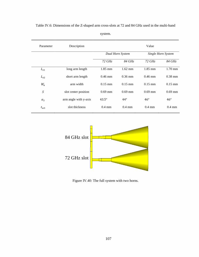
107

Table IV.6: Dimensions of the Z-shaped arm cross-slots at 72 and 84 GHz used in the multi-band

system.


Dual Horn System Single Horn System

72 GHz 84 GHz 72 GHz 84 GHz

𝑧1 long arm length 1.85 mm 1.62 mm 1.85 mm 1.70 mm

𝑧2 short arm length 0.46 mm 0.36 mm 0.46 mm 0.38 mm

𝑎 arm width 0.15 mm 0.15 mm 0.15 mm 0.15 mm

slot center position 0.69 mm 0.69 mm 0.69 mm 0.69 mm

𝛼2 arm angle with y-axis 43.5° 44° 46° 46°

𝑡𝑤3 slot thickness 0.4 mm 0.4 mm 0.4 mm 0.4 mm

Figure IV.40: The full system with two horns.

84 GHz slot

72 GHz slot

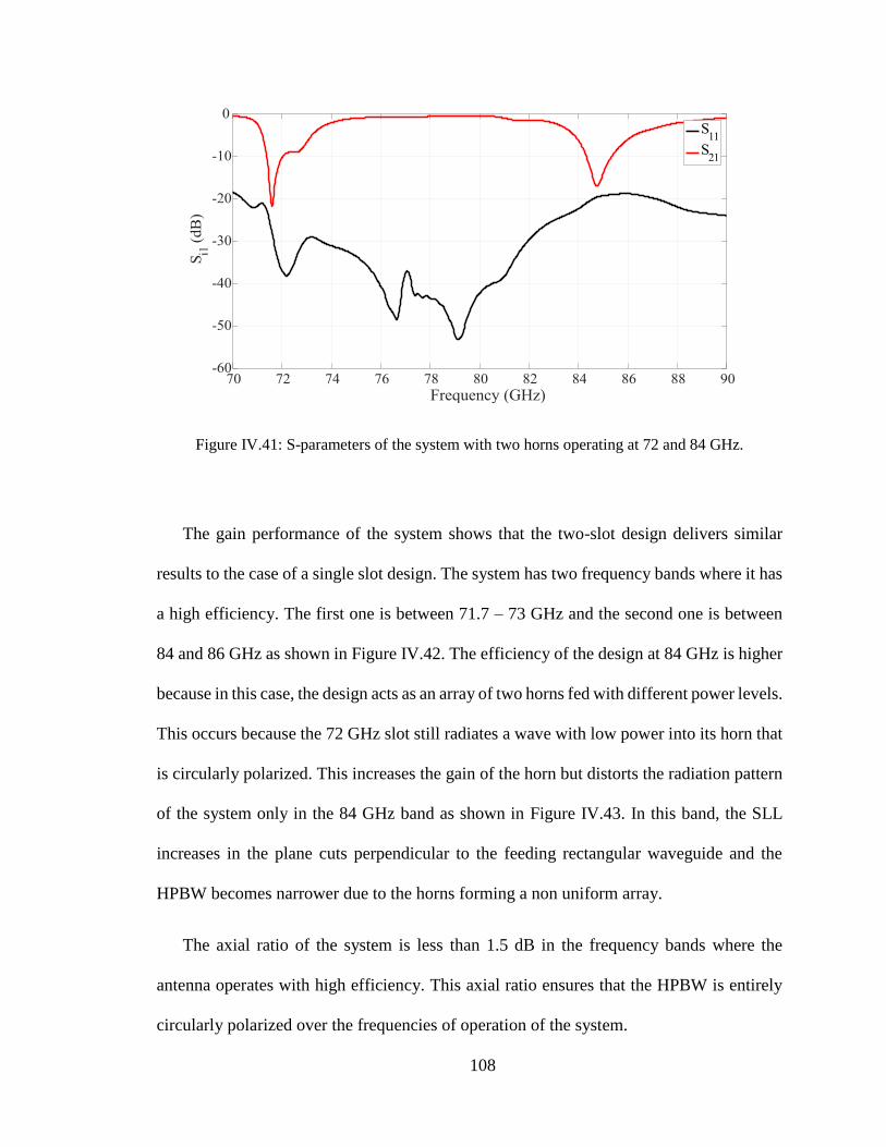
108

Figure IV.41: S-parameters of the system with two horns operating at 72 and 84 GHz.

The gain performance of the system shows that the two-slot design delivers similar

results to the case of a single slot design. The system has two frequency bands where it has

a high efficiency. The first one is between 71.7 – 73 GHz and the second one is between

84 and 86 GHz as shown in Figure IV.42. The efficiency of the design at 84 GHz is higher

because in this case, the design acts as an array of two horns fed with different power levels.

This occurs because the 72 GHz slot still radiates a wave with low power into its horn that

is circularly polarized. This increases the gain of the horn but distorts the radiation pattern

of the system only in the 84 GHz band as shown in Figure IV.43. In this band, the SLL

increases in the plane cuts perpendicular to the feeding rectangular waveguide and the

HPBW becomes narrower due to the horns forming a non uniform array.

The axial ratio of the system is less than 1.5 dB in the frequency bands where the

antenna operates with high efficiency. This axial ratio ensures that the HPBW is entirely

circularly polarized over the frequencies of operation of the system.

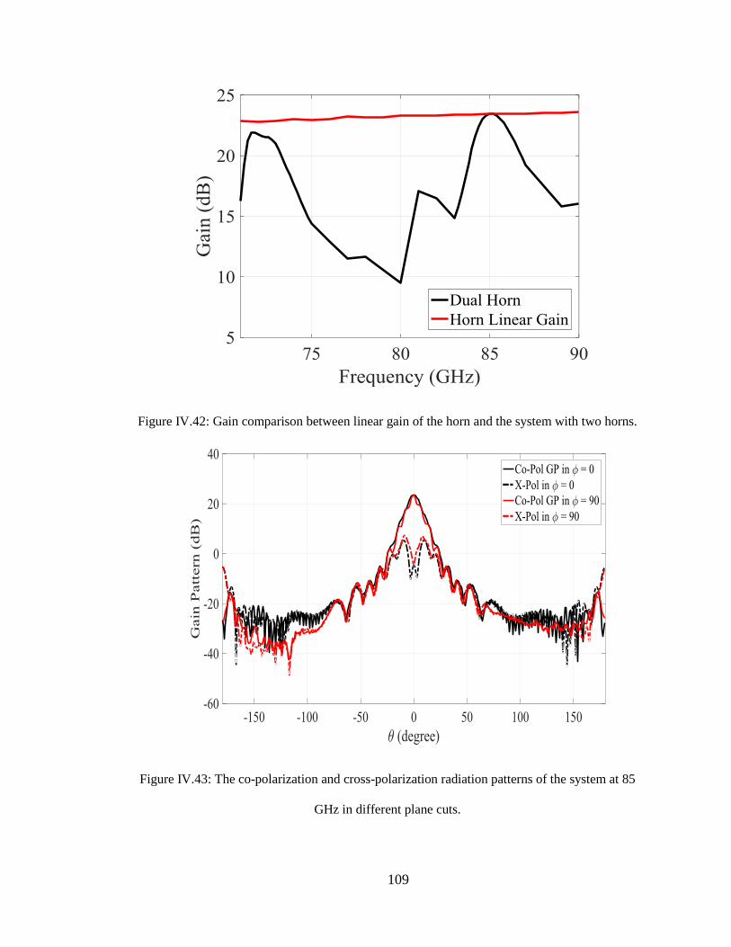
109

Figure IV.42: Gain comparison between linear gain of the horn and the system with two horns.

Figure IV.43: The co-polarization and cross-polarization radiation patterns of the system at 85

GHz in different plane cuts.

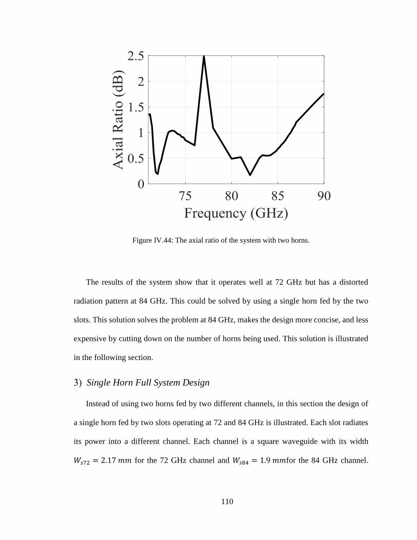
110

Figure IV.44: The axial ratio of the system with two horns.

The results of the system show that it operates well at 72 GHz but has a distorted

radiation pattern at 84 GHz. This could be solved by using a single horn fed by the two

slots. This solution solves the problem at 84 GHz, makes the design more concise, and less

expensive by cutting down on the number of horns being used. This solution is illustrated

in the following section.

Single Horn Full System Design

Instead of using two horns fed by two different channels, in this section the design of

a single horn fed by two slots operating at 72 and 84 GHz is illustrated. Each slot radiates

its power into a different channel. Each channel is a square waveguide with its width

72 = 2.17 𝑚𝑚 for the 72 GHz channel and 84 = 1.9 𝑚𝑚for the 84 GHz channel.

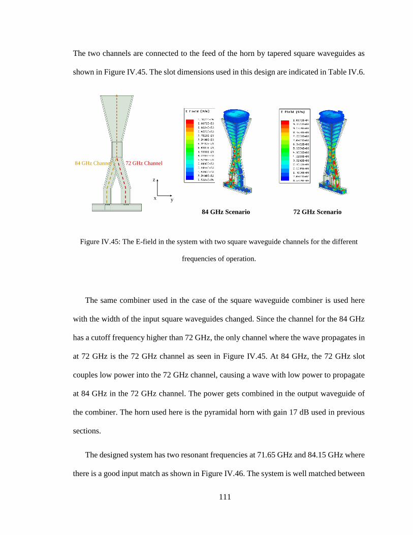
111

The two channels are connected to the feed of the horn by tapered square waveguides as

shown in Figure IV.45. The slot dimensions used in this design are indicated in Table IV.6.

Figure IV.45: The E-field in the system with two square waveguide channels for the different

frequencies of operation.

The same combiner used in the case of the square waveguide combiner is used here

with the width of the input square waveguides changed. Since the channel for the 84 GHz

has a cutoff frequency higher than 72 GHz, the only channel where the wave propagates in

at 72 GHz is the 72 GHz channel as seen in Figure IV.45. At 84 GHz, the 72 GHz slot

couples low power into the 72 GHz channel, causing a wave with low power to propagate

at 84 GHz in the 72 GHz channel. The power gets combined in the output waveguide of

the combiner. The horn used here is the pyramidal horn with gain 17 dB used in previous

sections.

The designed system has two resonant frequencies at 71.65 GHz and 84.15 GHz where

there is a good input match as shown in Figure IV.46. The system is well matched between

84 GHz Channel 72 GHz Channel

y

z

x

72 GHz Scenario84 GHz Scenario

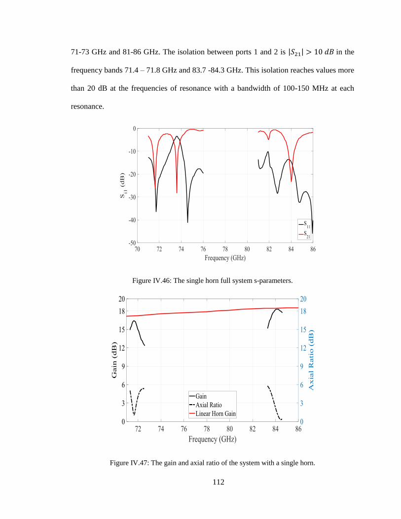
112

71-73 GHz and 81-86 GHz. The isolation between ports 1 and 2 is | 21| > 10 𝑑𝐵 in the

frequency bands 71.4 – 71.8 GHz and 83.7 -84.3 GHz. This isolation reaches values more

than 20 dB at the frequencies of resonance with a bandwidth of 100-150 MHz at each

resonance.

Figure IV.46: The single horn full system s-parameters.

Figure IV.47: The gain and axial ratio of the system with a single horn.

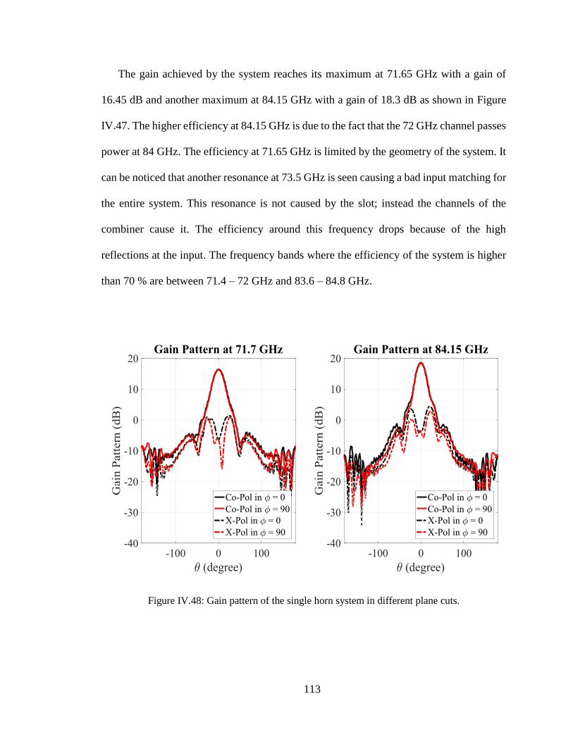
113

The gain achieved by the system reaches its maximum at 71.65 GHz with a gain of

16.45 dB and another maximum at 84.15 GHz with a gain of 18.3 dB as shown in Figure

IV.47. The higher efficiency at 84.15 GHz is due to the fact that the 72 GHz channel passes

power at 84 GHz. The efficiency at 71.65 GHz is limited by the geometry of the system. It

can be noticed that another resonance at 73.5 GHz is seen causing a bad input matching for

the entire system. This resonance is not caused by the slot; instead the channels of the

combiner cause it. The efficiency around this frequency drops because of the high

reflections at the input. The frequency bands where the efficiency of the system is higher

than 70 % are between 71.4 – 72 GHz and 83.6 – 84.8 GHz.

Figure IV.48: Gain pattern of the single horn system in different plane cuts.

114

The axial ratio in the direction of the highest gain is less than 3 dB in the frequency

bands of 71.45 – 71.9 GHz and of 84.85 – 84.6 GHz as shown in Figure IV.47. At 71.65

GHz and 84.4 GHz, the axial ratio reaches a minimum with a value of 0.9 dB and 0.3 dB

respectively. The system does not affect the radiation pattern of the horn. The HPBW is

still the same at with HPBW = 24. The SLL of the horn is at -27 dB in all plane cuts. The

HPBW of the horn is entirely circularly polarized at 71.7 GHz and 84.15 GHz in all plane

cuts as shown in Figure IV.48.

These results show that the system works at 71.7 and 84.15 GHz with a good bandwidth

of operation of 400 MHz and 900 MHz, respectively. The system can be used to feed any

horn and make it circularly polarized in those frequency bands.

IX. CONCLUSION

This chapter illustrated the design of the cross slot fed waveguide polarizer. Both a

circular waveguide and square waveguide were investigated as an extracting waveguide.

The power of multiple cross slots was combined to form a more efficient polarizer that has

a 70% efficiency bandwidth of 2.2% of the frequency band. This polarizer concept is also

used to design a multi band circularly polarized antenna system capable of providing either

LHCP or a RHCP by changing the feeding port.

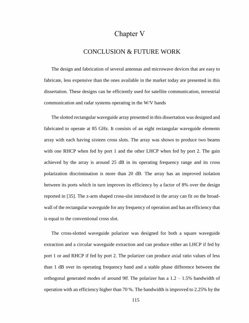
115

CONCLUSION & FUTURE WORK

The design and fabrication of several antennas and microwave devices that are easy to

fabricate, less expensive than the ones available in the market today are presented in this

dissertation. These designs can be efficiently used for satellite communication, terrestrial

communication and radar systems operating in the W/V bands

The slotted rectangular waveguide array presented in this dissertation was designed and

fabricated to operate at 85 GHz. It consists of an eight rectangular waveguide elements

array with each having sixteen cross slots. The array was shown to produce two beams

with one RHCP when fed by port 1 and the other LHCP when fed by port 2. The gain

achieved by the array is around 25 dB in its operating frequency range and its cross

polarization discrimination is more than 20 dB. The array has an improved isolation

between its ports which in turn improves its efficiency by a factor of 8% over the design

reported in [35]. The z-arm shaped cross-slot introduced in the array can fit on the broad-

wall of the rectangular waveguide for any frequency of operation and has an efficiency that

is equal to the conventional cross slot.

The cross-slotted waveguide polarizer was designed for both a square waveguide

extraction and a circular waveguide extraction and can produce either an LHCP if fed by

port 1 or and RHCP if fed by port 2. The polarizer can produce axial ratio values of less

than 1 dB over its operating frequency band and a stable phase difference between the

orthogonal generated modes of around 90. The polarizer has a 1.2 – 1.5% bandwidth of

operation with an efficiency higher than 70 %. The bandwidth is improved to 2.25% by the

116

use of square waveguide combiners that combine the power of different slots. The polarizer

has the ability to operate simultaneously at multiple frequency bands that are far away from

each other while producing a good axial ratio and an isolation between the feeding ports

that is more than 20 dB making it goof for radar applications.

A system that allows the activation of the different feeding ports of the cross slotted

rectangular waveguide array should be realized in the future. The fabrication of the square

waveguide combiner that is used to improve the cross slot polarizer should be fabricated

and tested. Finally, the design of the square waveguide combiner that operates at both 72

GHz and 84 GHz and the 23 dB pyramidal horn should be fabricated and tested.

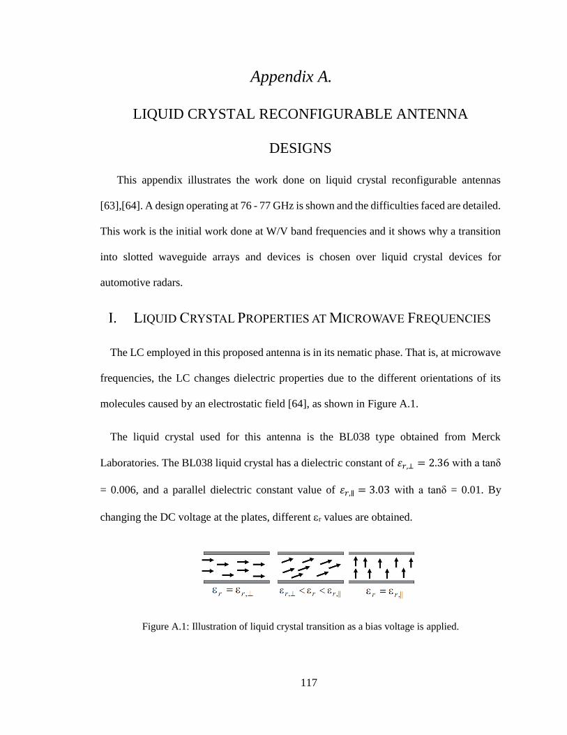
117

Appendix A.

LIQUID CRYSTAL RECONFIGURABLE ANTENNA

DESIGNS

This appendix illustrates the work done on liquid crystal reconfigurable antennas

[63],[64]. A design operating at 76 - 77 GHz is shown and the difficulties faced are detailed.

This work is the initial work done at W/V band frequencies and it shows why a transition

into slotted waveguide arrays and devices is chosen over liquid crystal devices for

automotive radars.

LIQUID CRYSTAL PROPERTIES AT MICROWAVE FREQUENCIES

The LC employed in this proposed antenna is in its nematic phase. That is, at microwave

frequencies, the LC changes dielectric properties due to the different orientations of its

molecules caused by an electrostatic field [64], as shown in Figure A.1.

The liquid crystal used for this antenna is the BL038 type obtained from Merck

Laboratories. The BL038 liquid crystal has a dielectric constant of 휀 ,⊥ = 2.36 with a tanδ

= 0.006, and a parallel dielectric constant value of 휀 ,∥ = 3.03 with a tanδ = 0.01. By

changing the DC voltage at the plates, different r values are obtained.

Figure A.1: Illustration of liquid crystal transition as a bias voltage is applied.

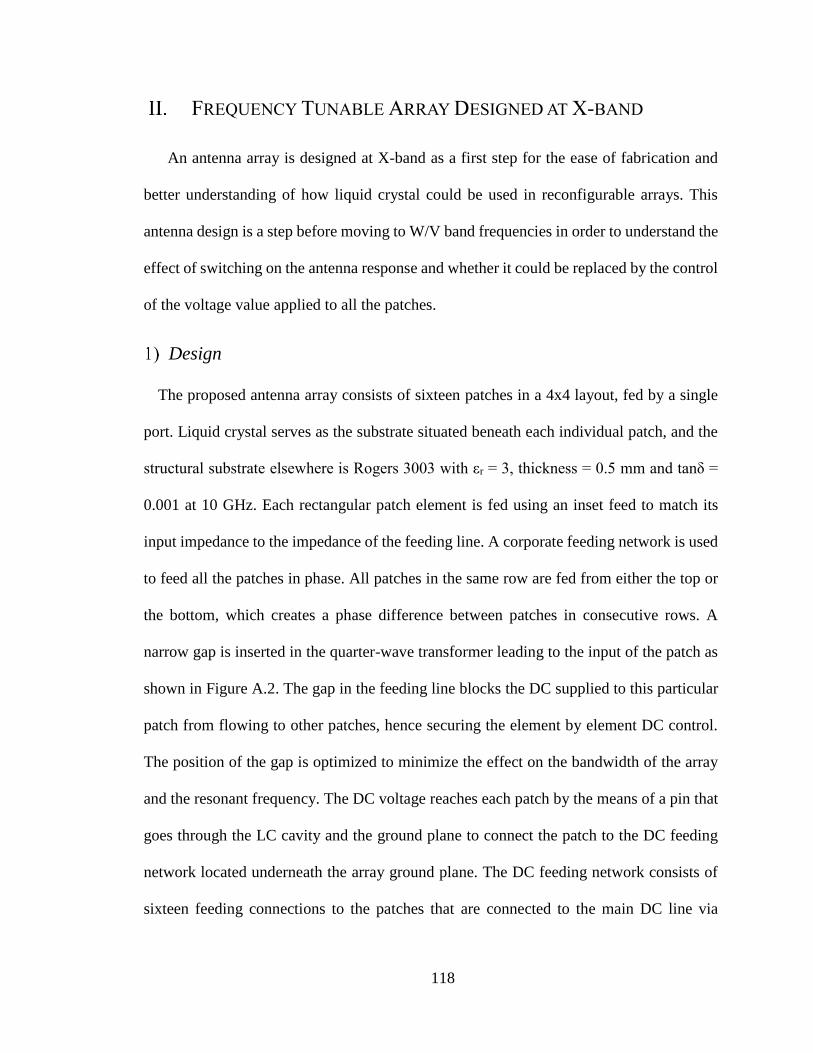
118

FREQUENCY TUNABLE ARRAY DESIGNED AT X-BAND

An antenna array is designed at X-band as a first step for the ease of fabrication and

better understanding of how liquid crystal could be used in reconfigurable arrays. This

antenna design is a step before moving to W/V band frequencies in order to understand the

effect of switching on the antenna response and whether it could be replaced by the control

of the voltage value applied to all the patches.

Design

The proposed antenna array consists of sixteen patches in a 4x4 layout, fed by a single

port. Liquid crystal serves as the substrate situated beneath each individual patch, and the

structural substrate elsewhere is Rogers 3003 with εr = 3, thickness = 0.5 mm and tanδ =

0.001 at 10 GHz. Each rectangular patch element is fed using an inset feed to match its

input impedance to the impedance of the feeding line. A corporate feeding network is used

to feed all the patches in phase. All patches in the same row are fed from either the top or

the bottom, which creates a phase difference between patches in consecutive rows. A

narrow gap is inserted in the quarter-wave transformer leading to the input of the patch as

shown in Figure A.2. The gap in the feeding line blocks the DC supplied to this particular

patch from flowing to other patches, hence securing the element by element DC control.

The position of the gap is optimized to minimize the effect on the bandwidth of the array

and the resonant frequency. The DC voltage reaches each patch by the means of a pin that

goes through the LC cavity and the ground plane to connect the patch to the DC feeding

network located underneath the array ground plane. The DC feeding network consists of

sixteen feeding connections to the patches that are connected to the main DC line via

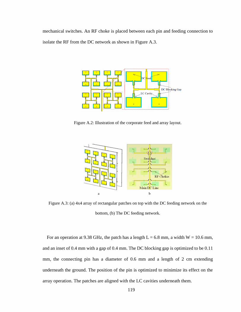
119

mechanical switches. An RF choke is placed between each pin and feeding connection to

isolate the RF from the DC network as shown in Figure A.3.

Figure A.2: Illustration of the corporate feed and array layout.

Figure A.3: (a) 4x4 array of rectangular patches on top with the DC feeding network on the

bottom, (b) The DC feeding network.

For an operation at 9.38 GHz, the patch has a length L = 6.8 mm, a width W = 10.6 mm,

and an inset of 0.4 mm with a gap of 0.4 mm. The DC blocking gap is optimized to be 0.11

mm, the connecting pin has a diameter of 0.6 mm and a length of 2 cm extending

underneath the ground. The position of the pin is optimized to minimize its effect on the

array operation. The patches are aligned with the LC cavities underneath them.

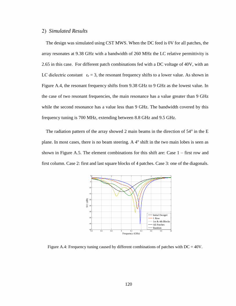
120

Simulated Results

The design was simulated using CST MWS. When the DC feed is 0V for all patches, the

array resonates at 9.38 GHz with a bandwidth of 260 MHz the LC relative permittivity is

2.65 in this case. For different patch combinations fed with a DC voltage of 40V, with an

LC dielectric constant εr = 3, the resonant frequency shifts to a lower value. As shown in

Figure A.4, the resonant frequency shifts from 9.38 GHz to 9 GHz as the lowest value. In

the case of two resonant frequencies, the main resonance has a value greater than 9 GHz

while the second resonance has a value less than 9 GHz. The bandwidth covered by this

frequency tuning is 700 MHz, extending between 8.8 GHz and 9.5 GHz.

The radiation pattern of the array showed 2 main beams in the direction of 54o in the E

plane. In most cases, there is no beam steering. A 4o shift in the two main lobes is seen as

shown in Figure A.5. The element combinations for this shift are: Case 1 – first row and

first column. Case 2: first and last square blocks of 4 patches. Case 3: one of the diagonals.

Figure A.4: Frequency tuning caused by different combinations of patches with DC = 40V.

8.4 8.6 8.8 9 9.2 9.4 9.6 9.8 10-45

-40

-35

-30

-25

-20

-15

-10

-5

0

Frequency (GHz)

S11 (

dB

)

Initial Design1

1 Row

1st & 4th Blocks

All Patches

Random

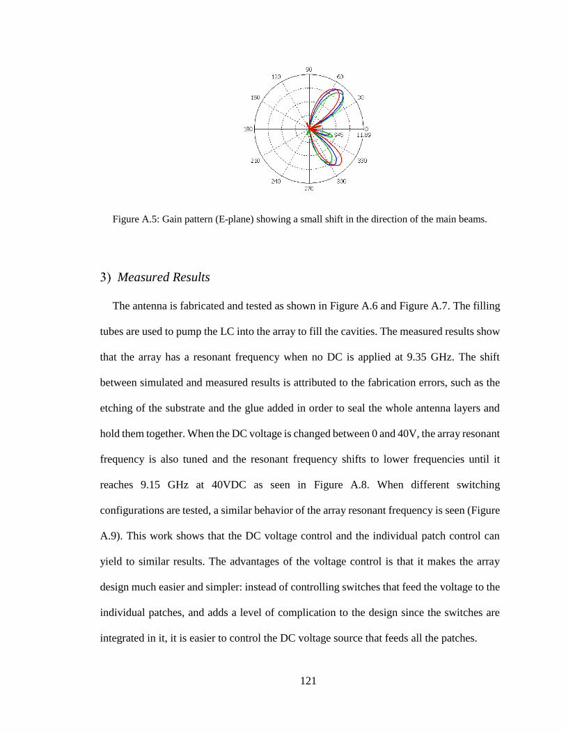
121

Figure A.5: Gain pattern (E-plane) showing a small shift in the direction of the main beams.

Measured Results

The antenna is fabricated and tested as shown in Figure A.6 and Figure A.7. The filling

tubes are used to pump the LC into the array to fill the cavities. The measured results show

that the array has a resonant frequency when no DC is applied at 9.35 GHz. The shift

between simulated and measured results is attributed to the fabrication errors, such as the

etching of the substrate and the glue added in order to seal the whole antenna layers and

hold them together. When the DC voltage is changed between 0 and 40V, the array resonant

frequency is also tuned and the resonant frequency shifts to lower frequencies until it

reaches 9.15 GHz at 40VDC as seen in Figure A.8. When different switching

configurations are tested, a similar behavior of the array resonant frequency is seen (Figure

A.9). This work shows that the DC voltage control and the individual patch control can

yield to similar results. The advantages of the voltage control is that it makes the array

design much easier and simpler: instead of controlling switches that feed the voltage to the

individual patches, and adds a level of complication to the design since the switches are

integrated in it, it is easier to control the DC voltage source that feeds all the patches.

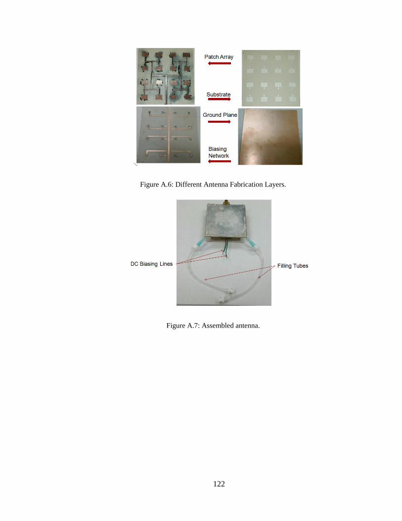
122

Figure A.6: Different Antenna Fabrication Layers.

Figure A.7: Assembled antenna.

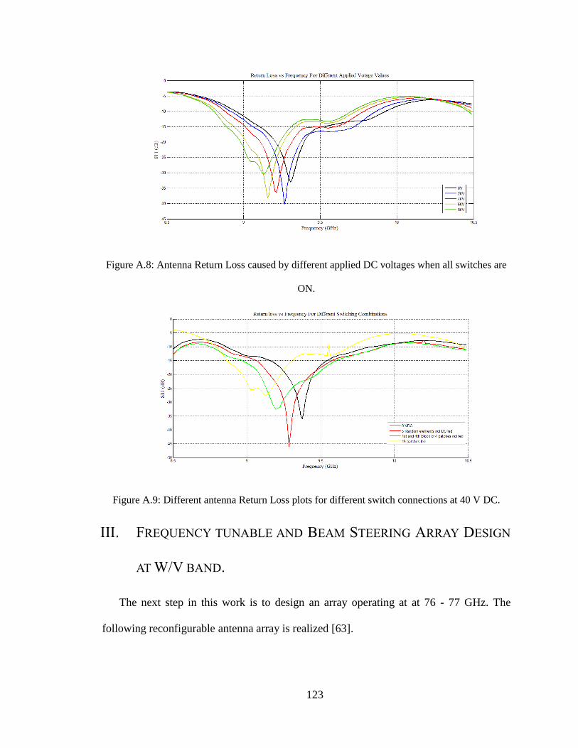
123

Figure A.8: Antenna Return Loss caused by different applied DC voltages when all switches are

ON.

Figure A.9: Different antenna Return Loss plots for different switch connections at 40 V DC.

FREQUENCY TUNABLE AND BEAM STEERING ARRAY DESIGN

AT W/V BAND.

The next step in this work is to design an array operating at at 76 - 77 GHz. The

following reconfigurable antenna array is realized [63].

124

Design

The proposed antenna array is composed of a total of three layers. The top layer consists

of eight rectangular patches in a 2x4 layout, fed by a single microstrip feed network. It is

important to indicate that each individual patch is fed by a uniform meander line of

impedance Z0 = 100Ω. Since the antenna operates in the W/V-band, a grounded CPW to

microstrip line transition (Figure A.10) or a rectangular waveguide to microstrip line

transition (Figure A.11) are used. The middle layer is composed of a Rogers 3003 substrate

with r=3, a thickness of 0.13 mm, and a tanδ of 0.001 at 70 GHz. The thickness of the

substrate is taken to be thin to ensure high speed switching of the incorporated LC in the

cavities. Within this layer, LC cavities are positioned underneath each individual patch.

Under each meander line feeding the individual patches there is an LC cavity. The meander

lines are used to control the phase at the input of each patch.

All patches in the same row are fed from either the top or the bottom, which creates a

phase difference of 180o between patches in different rows. The bottom layer of the array

is composed of the ground plane where a gap is inserted underneath each meandered line.

The gap insures the separation of DC voltage supplied to each row of meander lines.

By introducing the gaps in the ground plane, the radiation pattern is affected. To impede

such a consequence, a Rogers Ultralam Bondply 3850HT layer of thickness 25 µm is

added. A high impedance line is added to the main feed to connect it to the DC voltage

feeding network. A radial stub is also added to this line to ensure that RF signals do not

reach the DC feeding network.

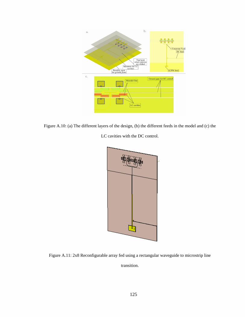
125

Figure A.10: (a) The different layers of the design, (b) the different feeds in the model and (c) the

LC cavities with the DC control.

Figure A.11: 2x8 Reconfigurable array fed using a rectangular waveguide to microstrip line

transition.

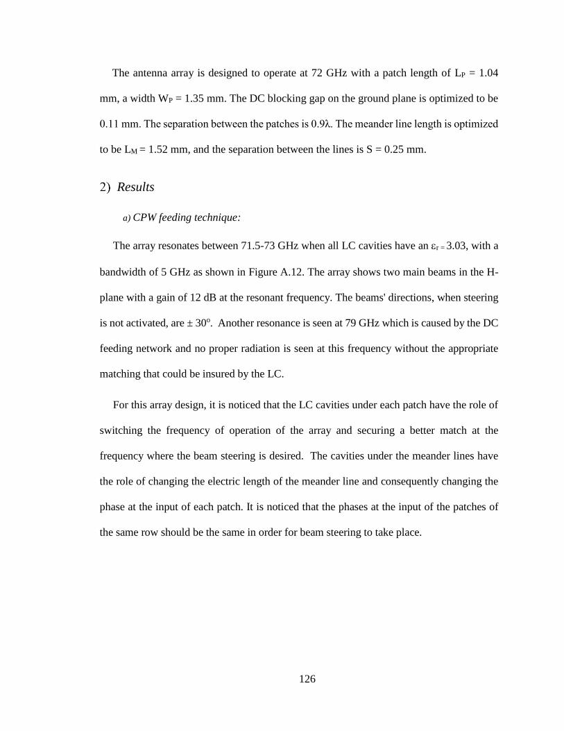
126

The antenna array is designed to operate at 72 GHz with a patch length of LP = 1.04

mm, a width WP = 1.35 mm. The DC blocking gap on the ground plane is optimized to be

0.11 mm. The separation between the patches is 0.9λ. The meander line length is optimized

to be LM = 1.52 mm, and the separation between the lines is S = 0.25 mm.

Results

a) CPW feeding technique:

The array resonates between 71.5-73 GHz when all LC cavities have an r = 3.03, with a

bandwidth of 5 GHz as shown in Figure A.12. The array shows two main beams in the H-

plane with a gain of 12 dB at the resonant frequency. The beams' directions, when steering

is not activated, are ± 30o. Another resonance is seen at 79 GHz which is caused by the DC

feeding network and no proper radiation is seen at this frequency without the appropriate

matching that could be insured by the LC.

For this array design, it is noticed that the LC cavities under each patch have the role of

switching the frequency of operation of the array and securing a better match at the

frequency where the beam steering is desired. The cavities under the meander lines have

the role of changing the electric length of the meander line and consequently changing the

phase at the input of each patch. It is noticed that the phases at the input of the patches of

the same row should be the same in order for beam steering to take place.

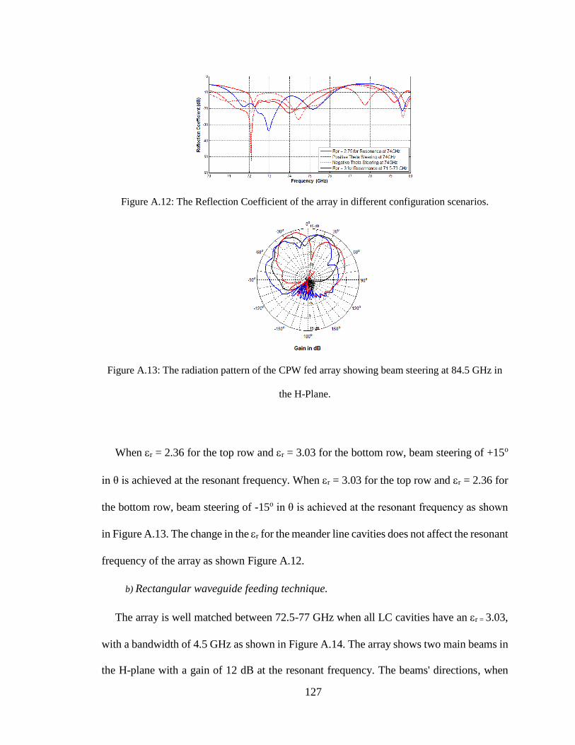
127

Figure A.12: The Reflection Coefficient of the array in different configuration scenarios.

Figure A.13: The radiation pattern of the CPW fed array showing beam steering at 84.5 GHz in

the H-Plane.

When r = 2.36 for the top row and r = 3.03 for the bottom row, beam steering of +15o

in θ is achieved at the resonant frequency. When r = 3.03 for the top row and r = 2.36 for

the bottom row, beam steering of -15o in θ is achieved at the resonant frequency as shown

in Figure A.13. The change in the r for the meander line cavities does not affect the resonant

frequency of the array as shown Figure A.12.

b) Rectangular waveguide feeding technique.

The array is well matched between 72.5-77 GHz when all LC cavities have an r = 3.03,

with a bandwidth of 4.5 GHz as shown in Figure A.14. The array shows two main beams in

the H-plane with a gain of 12 dB at the resonant frequency. The beams' directions, when

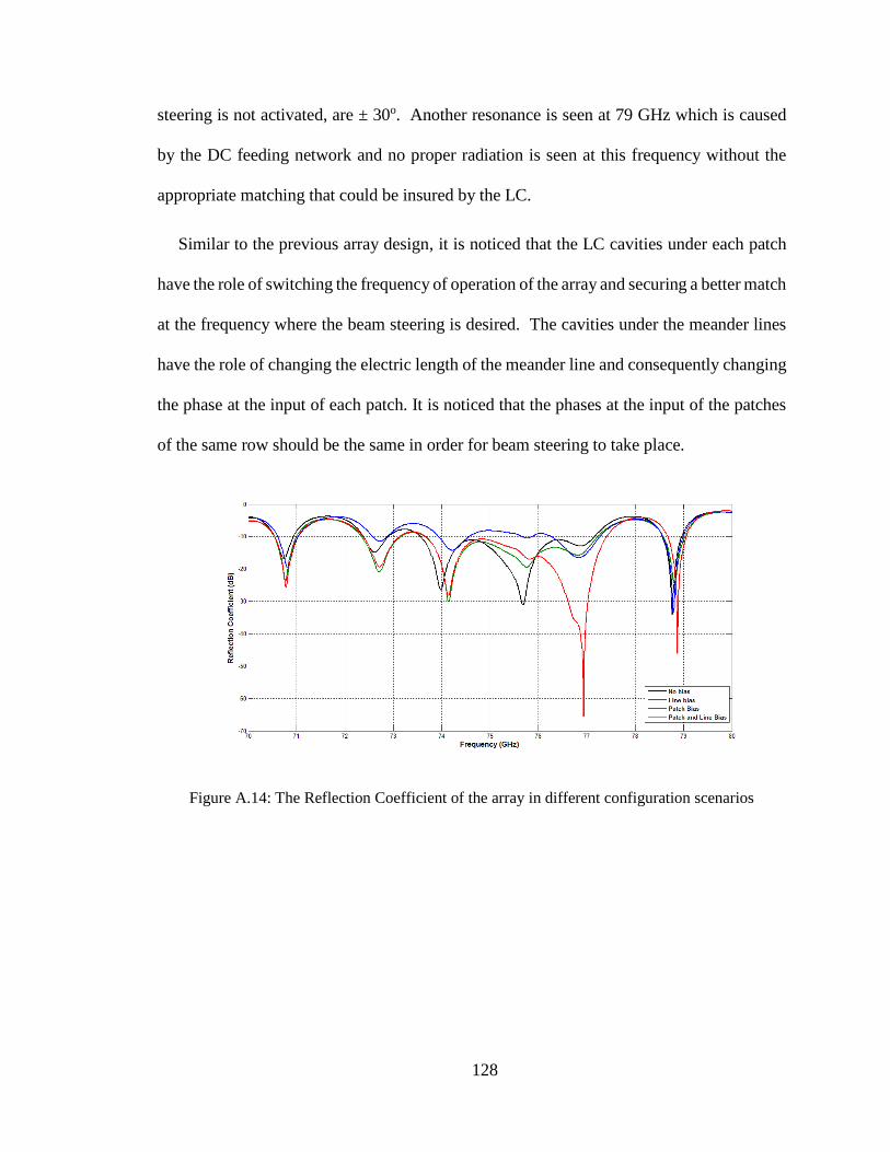
128

steering is not activated, are ± 30o. Another resonance is seen at 79 GHz which is caused

by the DC feeding network and no proper radiation is seen at this frequency without the

appropriate matching that could be insured by the LC.

Similar to the previous array design, it is noticed that the LC cavities under each patch

have the role of switching the frequency of operation of the array and securing a better match

at the frequency where the beam steering is desired. The cavities under the meander lines

have the role of changing the electric length of the meander line and consequently changing

the phase at the input of each patch. It is noticed that the phases at the input of the patches

of the same row should be the same in order for beam steering to take place.

Figure A.14: The Reflection Coefficient of the array in different configuration scenarios

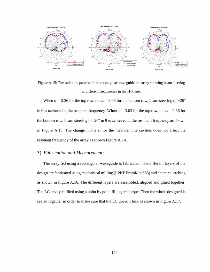
129

Figure A.15: The radiation pattern of the rectangular waveguide fed array showing beam steering

at different frequencies in the H-Plane.

When r = 2.36 for the top row and r = 3.03 for the bottom row, beam steering of +20o

in θ is achieved at the resonant frequency. When r = 3.03 for the top row and r = 2.36 for

the bottom row, beam steering of -20o in θ is achieved at the resonant frequency as shown

in Figure A.15. The change in the r for the meander line cavities does not affect the

resonant frequency of the array as shown Figure A.14.

Fabrication and Measurement:

The array fed using a rectangular waveguide is fabricated. The different layers of the

design are fabricated using mechanical milling (LPKF ProtoMat S63) and chemical etching

as shown in Figure A.16. The different layers are assembled, aligned and glued together.

The LC cavity is filled using a point by point filling technique. Then the whole designed is

sealed together in order to make sure that the LC doesn’t leak as shown in Figure A.17.

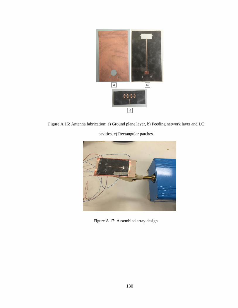
130

Figure A.16: Antenna fabrication: a) Ground plane layer, b) Feeding network layer and LC

cavities, c) Rectangular patches.

Figure A.17: Assembled array design.

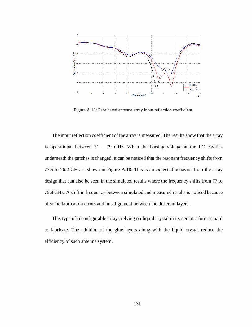
131

Figure A.18: Fabricated antenna array input reflection coefficient.

The input reflection coefficient of the array is measured. The results show that the array

is operational between 71 – 79 GHz. When the biasing voltage at the LC cavities

underneath the patches is changed, it can be noticed that the resonant frequency shifts from

77.5 to 76.2 GHz as shown in Figure A.18. This is an expected behavior from the array

design that can also be seen in the simulated results where the frequency shifts from 77 to

75.8 GHz. A shift in frequency between simulated and measured results is noticed because

of some fabrication errors and misalignment between the different layers.

This type of reconfigurable arrays relying on liquid crystal in its nematic form is hard

to fabricate. The addition of the glue layers along with the liquid crystal reduce the

efficiency of such antenna system.

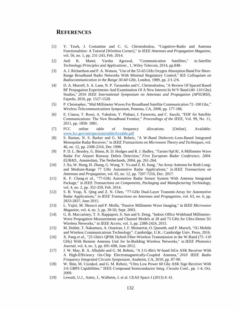
132

REFERENCES

[1] Y. Tawk, J. Costantine and C. G. Christodoulou, "Cognitive-Radio and Antenna

Functionalities: A Tutorial [Wireless Corner]," in IEEE Antennas and Propagation Magazine,

vol. 56, no. 1, pp. 231-243, Feb. 2014.

[2] Anil K. Maini; Varsha Agrawal, "Communication Satellites," in Satellite

Technology:Principles and Applications , 1, Wiley Telecom, 2014, pp.848-

[3] A. J. Richardson and P. A. Watson, "Use of the 55-65 GHz Oxygen Absorption Band For Short-

Range Broadband Radio Networks With Minimal Regulatory Control," IEE Colloquium on

Radiocommunication in the Range 30-60 GHz, London, 1989, pp. 2/1-2/6.

[4] D. A. Murrell, S. A. Lane, N. P. Tarasenko and C. Christodoulou, "A Review Of Spaced Based

RF Propagation Experiments And Examination Of A New Interest In W/V Band (40–110 Ghz)

Studies," 2016 IEEE International Symposium on Antennas and Propagation (APSURSI),

Fajardo, 2016, pp. 1527-1528.

[5] P. Christopher, “Mid Millimeter Waves For Broadband Satellite Communication 72–100 Ghz,”

Wireless Telecommunications Symposium, Pomona, CA, 2008, pp. 177-186.

[6] E. Cianca, T. Rossi, A. Yahalom, Y. Pinhasi, J. Farserotu, and C. Sacchi, “EHF for Satellite

Communications: The New Broadband Frontier,” Proceedings of the IEEE, Vol. 99, No. 11,

2011, pp. 1858- 1881.

[7] FCC online table of frequency allocations. [Online]. Available:

www.fcc.gov/oet/spectrum/table/fcctable.pdf

[8] S. Raman, N. S. Barker and G. M. Rebeiz, "A W-Band Dielectric-Lens-Based Integrated

Monopulse Radar Receiver," in IEEE Transactions on Microwave Theory and Techniques, vol.

46, no. 12, pp. 2308-2316, Dec 1998.

[9] P. D. L. Beasley, G. Binns, R. D. Hodges and R. J. Badley, "Tarsier/Spl R/, A Millimetre Wave

Radar For Airport Runway Debris Detection," First European Radar Conference, 2004.

EURAD., Amsterdam, The Netherlands, 2004, pp. 261-264.

[10] J. Xu, W. Hong, H. Zhang, G. Wang, Y. Yu and Z. H. Jiang, "An Array Antenna for Both Long-

and Medium-Range 77 GHz Automotive Radar Applications," in IEEE Transactions on

Antennas and Propagation, vol. 65, no. 12, pp. 7207-7216, Dec. 2017.

[11] K. F. Chang et al., "77-GHz Automotive Radar Sensor System With Antenna Integrated

Package," in IEEE Transactions on Components, Packaging and Manufacturing Technology,

vol. 4, no. 2, pp. 352-359, Feb. 2014.

[12] S. B. Yeap, X. Qing and Z. N. Chen, "77-GHz Dual-Layer Transmit-Array for Automotive

Radar Applications," in IEEE Transactions on Antennas and Propagation, vol. 63, no. 6, pp.

2833-2837, June 2015.

[13] L. Yujiri, M. Shoucri and P. Moffa, "Passive Millimeter Wave Imaging," in IEEE Microwave

Magazine, vol. 4, no. 3, pp. 39-50, Sept. 2003.

[14] G. R. Maccartney, T. S. Rappaport, S. Sun and S. Deng, "Indoor Office Wideband Millimeter-

Wave Propagation Measurements and Channel Models at 28 and 73 GHz for Ultra-Dense 5G

Wireless Networks," in IEEE Access, vol. 3, pp. 2388-2424, 2015.

[15] M. Dohler, T. Nakamura, A. Osseiran, J. F. Monserrat, O. Queseth, and P. Marsch, “5G Mobile

and Wireless Communications Technology”. Cambridge, U.K.: Cambridge Univ. Press, 2016.

[16] X. Pang et al., "25 Gbit/s QPSK Hybrid Fiber-Wireless Transmission in the W-Band (75–110

GHz) With Remote Antenna Unit for In-Building Wireless Networks," in IEEE Photonics

Journal, vol. 4, no. 3, pp. 691-698, June 2012.

[17] J. W. May, R. A. Alhalabi and G. M. Rebeiz, "A 3 G-Bit/s W-band SiGe ASK Receiver With

A High-Efficiency On-Chip Electromagnetically-Coupled Antenna," 2010 IEEE Radio

Frequency Integrated Circuits Symposium, Anaheim, CA, 2010, pp. 87-90.

[18] W. Shin, M. Uzonkol, and G. M. Rebeiz, “Ultra Low Power 60 Ghz ASK Sige Receiver With

3-6 GBPS Capabilities,” IEEE Compound Semiconductor Integ. Circuits Conf., pp. 1-4, Oct.

2009.

[19] Lewark, U.J., Antes, J., Walheim, J. et al. CEAS Space J (2013) 4: 41.

http://www.fcc.gov/oet/spectrum/table/fcctable.pdf

133

[20] A. Jebril, M. Lucente, M. Ruggieri and T. Rossi, "WAVE - A New Satellite Mission In W-

Band," 2005 IEEE Aerospace Conference, Big Sky, MT, 2005, pp. 870-879.

[21] Riva, C., Capsoni, C., Luini, L., Luccini, M., Nebuloni, R. and Martellucci, A. (2014), “The

Challenge Of Using The W Band In Satellite Communication”. Int. J. Satell. Commun.

Network., 32: 187–200.

[22] N. P. Tarasenko et al., "W/V-Band Terrestrial Link Experiment, an Overview," 2016 IEEE

International Symposium on Antennas and Propagation (APSURSI), Fajardo, 2016, pp. 1259-

1260.

[23] M. Zemba, J. Nessel, J. Houts, N. Tarasenko, S. Lane and D. Murrell, "Preliminary Results

From The AFRL-NASA W/V-Band Terrestrial Link Experiment In Albuquerque, NM," 2016

IEEE International Symposium on Antennas and Propagation (APSURSI), Fajardo, 2016, pp.

1249-1250.

[24] E. Amyotte et al., "Recent Developments In Ka-Band Satellite Antennas For Broadband

Communications," Proceedings of the Fourth European Conference on Antennas and

Propagation, Barcelona, 2010, pp. 1-5.

[25] S. W. Wang, C. H. Chien, C. L. Wang and R. B. Wu, "A Circular Polarizer Designed With A

Dielectric Septum Loading," in IEEE Transactions on Microwave Theory and Techniques, vol.

52, no. 7, pp. 1719-1723, July 2004.

[26] D. R. Hill, "Circularly Polarised Radiation From Narrow Wall Slots In Rectangular

Waveguide", Electronics Letters, vol. 16, no. 14, pp. 559-560, July 3 1980.

[27] M. Armstrong and N. Alexopoulos, "On The Design Of A Circularly Polarized Waveguide

Narrow Wall Linear Array", IEEE Transactions on Antennas and Propagation, vol. 23, no. 2,

pp. 244-250, Mar 1975.

[28] K. S. Min, J. Hirokawa, K. Sakurai, M. Ando and N. Goto, "Single-Layer Dipole Array For

Linear-To-Circular Polarisation Conversion Of Slotted Waveguide Array," in IEE Proceedings

- Microwaves, Antennas and Propagation, vol. 143, no. 3, pp. 211-216, Jun 1996.

[29] M. Ferrando-Rocher, J. I. Herranz-Herruzo, A. Valero-Nogueira and V. M. Rodrigo,

"Circularly Polarized Slotted Waveguide Array With Improved Axial Ratio Performance," in

IEEE Transactions on Antennas and Propagation, vol. 64, no. 9, pp. 4144-4148, Sept. 2016.

[30] D. Dogan and C. B. Top, "Circularly Polarized Ka-Band Waveguide Slot Array With Low

Sidelobes," 2012 6th European Conference on Antennas and Propagation (EUCAP), Prague,

2012, pp. 1105-1109.

[31] G. Montisci, "Design of Circularly Polarized Waveguide Slot Linear Arrays," in IEEE

Transactions on Antennas and Propagation, vol. 54, no. 10, pp. 3025-3029, Oct. 2006.

[32] P. Chen, W. Hong, Z. Kuai and J. Xu, "A Substrate Integrated Waveguide Circular Polarized

Slot Radiator and Its Linear Array," in IEEE Antennas and Wireless Propagation Letters, vol.

8, no. , pp. 120-123, 2009.

[33] M. Al Sharkawy and A. A. Kishk, "Wideband Beam-Scanning Circularly Polarized Inclined

Slots Using Ridge Gap Waveguide," in IEEE Antennas and Wireless Propagation Letters, vol.

13, no. , pp. 1187-1190, 2014.

[34] A. Simmons, "Circularly Polarized Slot Radiators," in IRE Transactions on Antennas and

Propagation, vol. 5, no. 1, pp. 31-36, January 1957.

[35] K. Sakakibara, Y. Kimura, J. Hirokawa, M. Ando and N. Goto, "A Two-Beam Slotted Leaky

Waveguide Array For Mobile Reception Of Dual-Polarization DBS," in IEEE Transactions on

Vehicular Technology, vol. 48, no. 1, pp. 1-7, Jan 1999.

[36] J. Hirokawa, K. Sakurai, M. Ando and N. Goto, "Matching Slot Pair For A Circularly-Polarised

Slotted Waveguide Array," in IEE Proceedings H - Microwaves, Antennas and Propagation,

vol. 137, no. 6, pp. 367-371, Dec 1990.

[37] S. Chatterjee, J. Das and A. Majumder, "Circularly Polarized Offset Center Cross Slotted Array

Antenna At Ka Band,"; 2016 IEEE MTT-S International Conference on Numerical

Electromagnetic and Multiphysics Modeling and Optimization (NEMO), Beijing, 2016, pp. 1-

4.

134

[38] A. Seaton and G. Carnegis, "A Novel Circularly Polarized Planar Array For Surveyor,"; 1958

IRE International Convention Record, New York, NY, USA, 1963, pp. 2-9.

[39] H. Bayer, A. Krauss, T. Zaiczek, R. Stephan, O. Enge-Rosenblatt and M. A. Hein, "Ka-Band

User Terminal Antennas for Satellite Communications [Antenna Applications Corner]," in

IEEE Antennas and Propagation Magazine, vol. 58, no. 1, pp. 76-88, Feb. 2016.

[40] C. A. Leal-Sevillano, J. R. Montejo-Garai, J. M. Rebollar and J. A. Ruiz-Cruz, "CAD For Dual-

Band Polarizers In Corrugated Rectangular Waveguide," 2011 41st European Microwave

Conference, Manchester, 2011, pp. 822-825.

[41] U. Tucholke, F. Arndt and T. Wriedt, "Field Theory Design of Square Waveguide Iris

Polarizers," in IEEE Transactions on Microwave Theory and Techniques, vol. 34, no. 1, pp.

156-160, Jan 1986.

[42] G. Virone, R. Tascone, M. Baralis, O. A. Peverini, A. Olivieri and R. Orta, "A Novel Design

Tool For Waveguide Polarizers," in IEEE Transactions on Microwave Theory and Techniques,

vol. 53, no. 3, pp. 888-894, March 2005.

[43] J. M. Rebollar and J. de Frutos, "Dual-Band Compact Square Waveguide Corrugated

Polarizer," IEEE Antennas and Propagation Society International Symposium. 1999 Digest.

Held in conjunction with: USNC/URSI National Radio Science Meeting (Cat. No.99CH37010),

Orlando, FL, USA, 1999, pp. 962-965 vol.2.

[44] G. Bertin, B. Piovano, L. Accatino and M. Mongiardo, "Full-Wave Design And Optimization

Of Circular Waveguide Polarizers With Elliptical Irises," in IEEE Transactions on Microwave

Theory and Techniques, vol. 50, no. 4, pp. 1077-1083, Apr 2002.

[45] Shih-Wei Wang, Chih-Hung Chien, Chun-Long Wang and Ruey-Beei Wu, "A Circular

Polarizer Designed With A Dielectric Septum Loading," in IEEE Transactions on Microwave

Theory and Techniques, vol. 52, no. 7, pp. 1719-1723, July 2004.

[46] Quinstar Linear to Circular fixed Polarizers [Online]. Website:

http://quinstar.com/shop/antenna-products/linear-to-circular-fixed-and-switchable-

polarizers/linear-to-circular-fixed-polarizers-qwl/

[47] Ming Chen and G. Tsandoulas, "A Wide-Band Square-Waveguide Array Polarizer," in IEEE

Transactions on Antennas and Propagation, vol. 21, no. 3, pp. 389-391, May 1973.

[48] B. Piovano, G. Bertin, L. Accatino and M. Mongiardo, "CAD and Optimization of Compact

Wide-band Septum Polarizers," 1999 29th European Microwave Conference, Munich,

Germany, 1999, pp. 235-238.

[49] J. Bornemann and V. A. Labay, "Ridge Waveguide Polarizer With Finite And Stepped-

Thickness Septum," in IEEE Transactions on Microwave Theory and Techniques, vol. 43, no.

8, pp. 1782-1787, Aug 1995.

[50] R. Ihmels, U. Papziner and F. Arndt, "Field Theory Design Of A Corrugated Septum

OMT," 1993 IEEE MTT-S International Microwave Symposium Digest, Atlanta, GA, USA,

1993, pp. 909-912 vol.2.

[51] J. A. Ruiz-Cruz, M. M. Fahmi, S. A. Fouladi and R. R. Mansour, "Waveguide Antenna Feeders

With Integrated Reconfigurable Dual Circular Polarization," in IEEE Transactions on

Microwave Theory and Techniques, vol. 59, no. 12, pp. 3365-3374, Dec. 2011.

[52] Kaiden, M., Kimura, K., Ogawa, H. et al. J Infrared Milli Terahz Waves (2009) 30: 727

[53] M. J. Franco, "A High-Performance Dual-Mode Feed Horn for Parabolic Reflectors with a

Stepped-Septum Polarizer in a Circular Waveguide [Antenna Designer's Notebook]," in IEEE

Antennas and Propagation Magazine, vol. 53, no. 3, pp. 142-146, June 2011.

[54] C. A. Leal-Sevillano, K. B. Cooper, J. A. Ruiz-Cruz, J. R. Montejo-Garai and J. M. Rebollar,

"A 225 GHz Circular Polarization Waveguide Duplexer Based on a Septum Orthomode

Transducer Polarizer," in IEEE Transactions on Terahertz Science and Technology, vol. 3, no.

5, pp. 574-583, Sept. 2013.

[55] F.N. Ayoub, Y. Tawk, E. Ardelean, J. Costantine, S. Lane, C. G. Christodoulou, “A Dual

Circularly Polarized Slotted Waveguide Array for W-Band Systems”, submitted to IEEE

Transactions on Antennas and Propagation.

http://quinstar.com/shop/antenna-products/linear-to-circular-fixed-and-switchable-polarizers/linear-to-circular-fixed-polarizers-qwl/

http://quinstar.com/shop/antenna-products/linear-to-circular-fixed-and-switchable-polarizers/linear-to-circular-fixed-polarizers-qwl/

135

[56] F. N. Ayoub, Y. Tawk, J. Costantine, C. G. Christodoulou, E. Ardelean, S.Lane, "2-D Cross

Slotted W-Band Waveguides Array", 2017 IEEE Antennas and Propagation Society

International Symposium (APSURSI), San Diego.

[57] Z. C. Hao, M. He, K. Fan and G. Luo, “A Planar Broadband Antenna for the E-Band Gigabyte

Wireless Communication”; in IEEE Transactions on Antennas and Propagation, vol. 65, no. 3,

pp. 1369-1373, March 2017.

[58] D. y. Kim, Y. Lim, H. S. Yoon and S. Nam, “High-Efficiency W-Band Electroforming Slot

Array Antenna”; in IEEE Transactions on Antennas and Propagation, vol. 63, no. 4, pp. 1854-

1857, April 2015.

[59] T. Li, H. Meng and W. Dou, “Design and Implementation of Dual-Frequency Dual-Polarization

Slotted Waveguide Antenna Array for Ka-Band Application”; in IEEE Antennas and Wireless

Propagation Letters, vol. 13, no. , pp. 1317-1320, 2014.

[60] A. P. King, "The Radiation Characteristics of Conical Horn Antennas," in Proceedings of the

IRE, vol. 38, no. 3, pp. 249-251, March 1950.

[61] C.A. Balanis, “Horn Antennas” in Antenna Theory: Analysis and Design, 4th ed. Hoboken,

New Jersey, USA: Wiley, 2016, ch. 13, pp. 754–757.

[62] Guardiola, Marta & Monsalve, Beatriz & Calafell, Irena & Roqueta, Gemma & Romeu, Jordi.

(2012). “Fabrication and Measurement of Homemade Standard Antennas.”, IEEE Antennas and

Propagation Magazine. 54. 177-194.

[63] F. N. Ayoub, Y. Tawk, J. Costantine, C. G. Christodoulou, S.Lane, D. Murell, "W/V-band

Reconfigurable Array Using Highly Anisotropic Liquid Crystals," 2016 IEEE Antennas and

Propagation Society International Symposium (APSURSI), Puerto Rico.

[64] F. N. Ayoub, C. D. Woehrle, Y. Tawk, D. T. Doyle, C. G. Christodoulou and J. Costantine,

"Frequency-tunable patch array using highly anisotropic liquid crystal," 2014 IEEE Antennas

and Propagation Society International Symposium (APSURSI), Memphis, TN, 2014, pp. 1664-

1665.

Documents

ANTENNAS FOR WV BAND APPLICATIONS