Embed Size (px)
Citation preview
UWB Antennas & Measurements
Gabriela QuinteroMICS UWB Network Meeting
11/12/2007
Outline
UWB Antenna AnalysisFrequency DomainTime Domain
Measurement TechniquesPeak and Average Power MeasurementsSpectrum Analyzer Settings
Fourier SeriesFourier Transform
UWB Measurements
Outline
UWB Antenna AnalysisFrequency DomainTime Domain
Measurement TechniquesPeak and Average Power MeasurementsSpectrum Analyzer Settings
Fourier SeriesFourier Transform
UWB Measurements
UWB Antennas
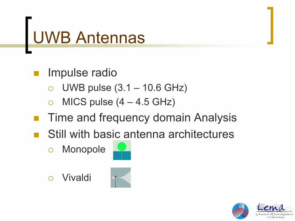
Impulse radioUWB pulse (3.1 – 10.6 GHz)MICS pulse (4 – 4.5 GHz)
Time and frequency domain AnalysisStill with basic antenna architectures
Monopole
Vivaldi
Time and Frequency Domain
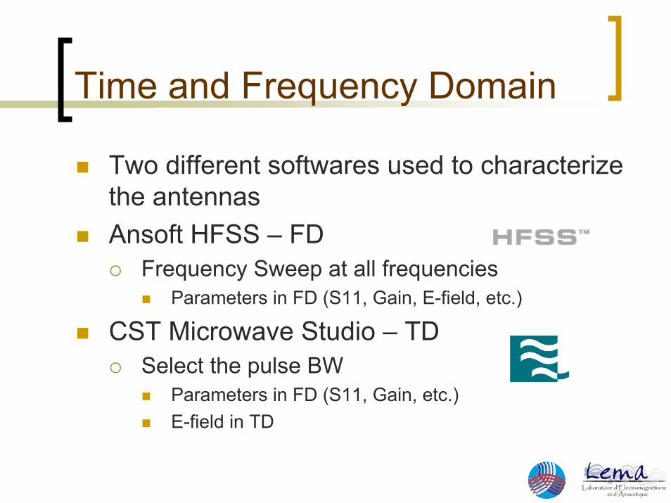
Two different softwares used to characterize the antennasAnsoft HFSS – FD
Frequency Sweep at all frequenciesParameters in FD (S11, Gain, E-field, etc.)
CST Microwave Studio – TDSelect the pulse BW
Parameters in FD (S11, Gain, etc.)E-field in TD
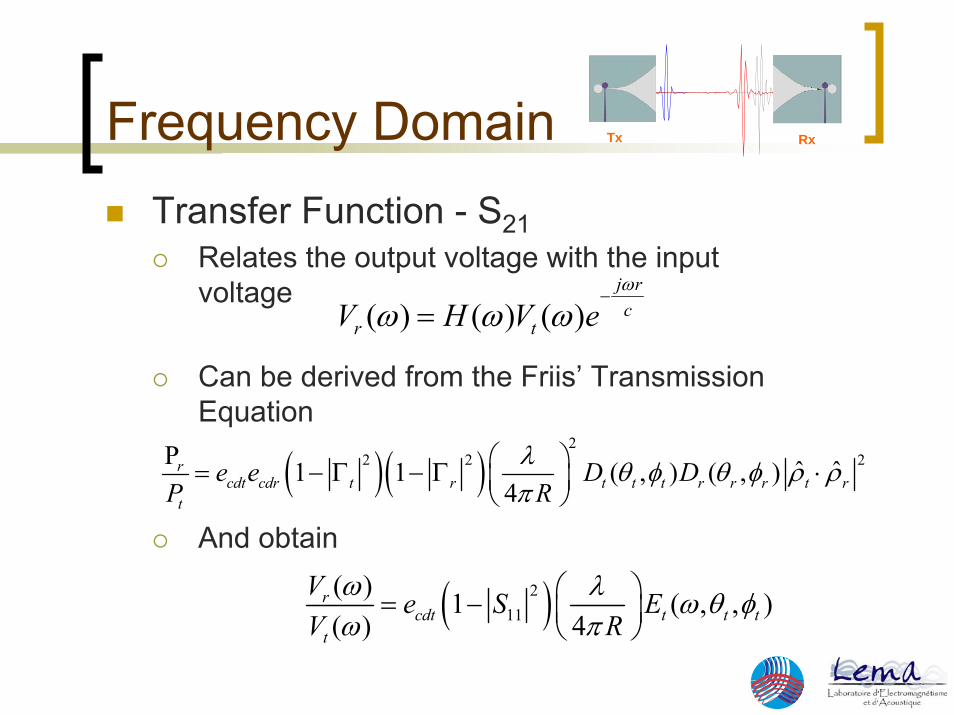
Frequency DomainTransfer Function - S21
Relates the output voltage with the input voltage
Can be derived from the Friis’ Transmission Equation
And obtain
( ) ( ) ( )j rc
r tV H V eω
ω ω ω−
=
( )( )2
2 2P ˆ ˆ1 1 ( , ) ( , )4
rcdt cdr t r t t t r r r t
t
e e D DP R
λ 2rθ φ θ φ ρ
π⎛ ⎞= − Γ − Γ ⎜ ⎟⎝ ⎠
ρ⋅
( )211
( ) 1 ( , , )( ) 4
rcdt t t t
t
V e S EV R
ω λ ω θ φω π
⎛ ⎞= − ⎜ ⎟⎝ ⎠
Tx Rx
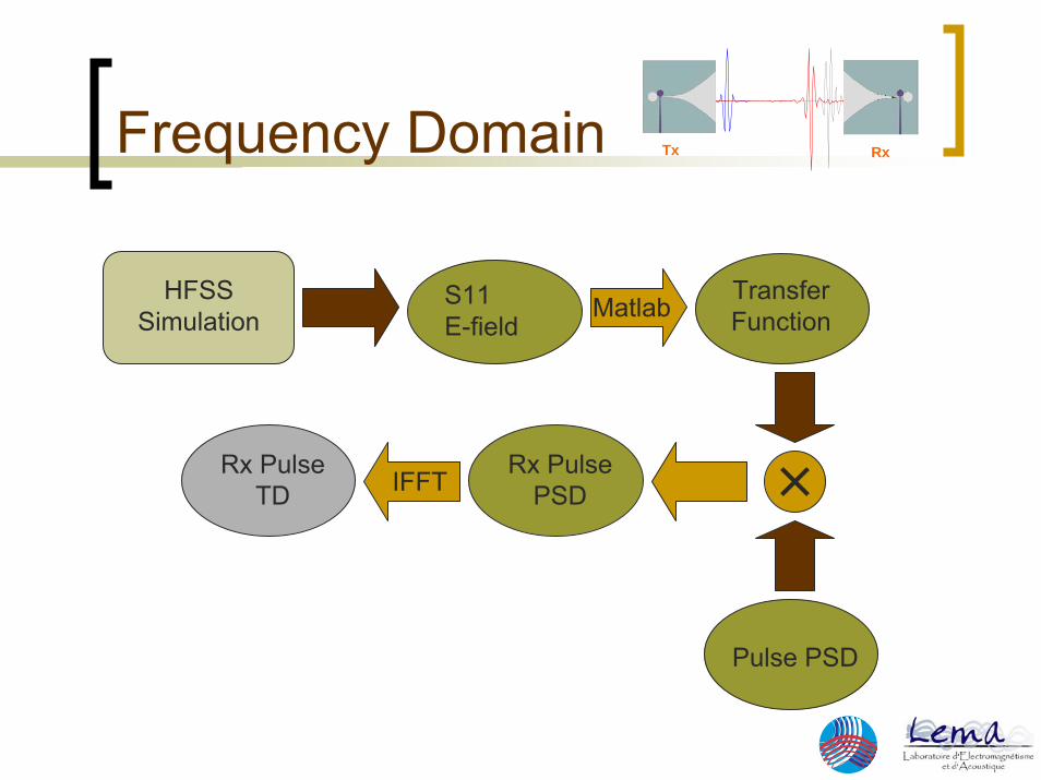
Frequency Domain
HFSS Simulation
S11 E-field
Transfer FunctionMatlab
Pulse PSD
Rx Pulse PSDIFFT
Rx Pulse TD
Tx Rx
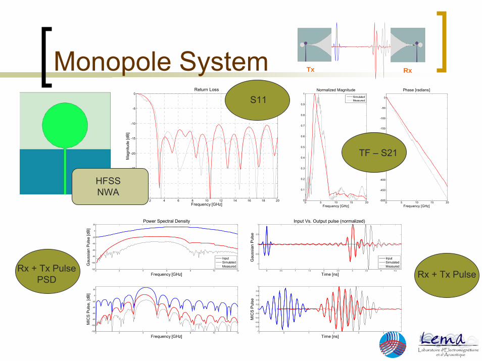
Monopole System
0 2 4 6 8 10 12 14 16 18 20-35
-30
-25
-20
-15
-10
-5
0Return Loss
Frequency [GHz]
Mag
nitu
de [d
B]
SimulatedMeasured
0 5 10 15 200
0.1
0.2
0.3
0.4
0.5
0.6
0.7
0.8
0.9
1Normalized Magnitude
Frequency [GHz]
SimulatedMeasured
0 5 10 15 20-500
-450
-400
-350
-300
-250
-200
-150
-100
-50
0
Frequency [GHz]
Phase [radians]
S11
HFSSNWA
TF – S21
Rx + Tx Pulse PSD Rx + Tx Pulse0 2 4 6 8 10 12
-120
-100
-80
-60
-40
-20
0
20
Frequency [GHz]
Gau
ssia
n Pu
lse
[dB]
Power Spectral Density
0 2 4 6 8 10 12-120
-100
-80
-60
-40
-20
0
20
MIC
S Pu
lse,
[dB]
Frequency [GHz]
InputSimulatedMeasured
0 0.5 1 1.5 2 2.5 3 3.5 4 4.5
-1
-0.5
0
0.5
1
Time [ns]
Gau
ssia
n Pu
lse
Input Vs. Output pulse (normalized)
-1 0 1 2 3 4-1
-0.8
-0.6
-0.4
-0.2
0
0.2
0.4
0.6
0.8
1
MIC
S Pu
lse
Time [ns]
InputSimulatedMeasured
Tx Rx
0 5 10 15 200
0.1
0.2
0.3
0.4
0.5
0.6
0.7
0.8
0.9
1Normalized Magnitude
Frequency [GHz]
SimulatedMeasured
0 5 10 15 20-500
-450
-400
-350
-300
-250
-200
-150
-100
-50
0
Frequency [GHz]
Phase [radians]
0 2 4 6 8 10 12 14 16 18 20-35
-30
-25
-20
-15
-10
-5
0Return Loss
Frequency [GHz]
Mag
nitu
de [d
B]
SimulatedMeasured
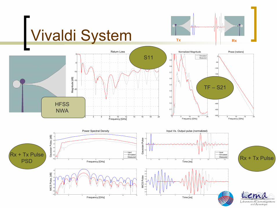
Vivaldi SystemS11
HFSSNWA
TF – S21
Rx + Tx Pulse0 2 4 6 8 10 12-120
-100
-80
-60
-40
-20
0
20
Frequency [GHz]
Gau
ssia
n Pu
lse,
[dB]
Power Spectral Density
InputSimulatedMeasured
0 2 4 6 8 10 12-120
-100
-80
-60
-40
-20
0
20
MIC
S Pu
lse,
[dB]
Frequency [GHz]
Rx + Tx Pulse PSD 0 0.5 1 1.5 2 2.5 3 3.5 4 4.5
-1
-0.5
0
0.5
1
Time [ns]
Gau
ssia
n Pu
lse
Input Vs. Output pulse (normalized)
InputSimulatedMeasured
-1 0 1 2 3 4-1
-0.8
-0.6
-0.4
-0.2
0
0.2
0.4
0.6
0.8
1
MIC
S Pu
lse
Time [ns]
Tx Rx
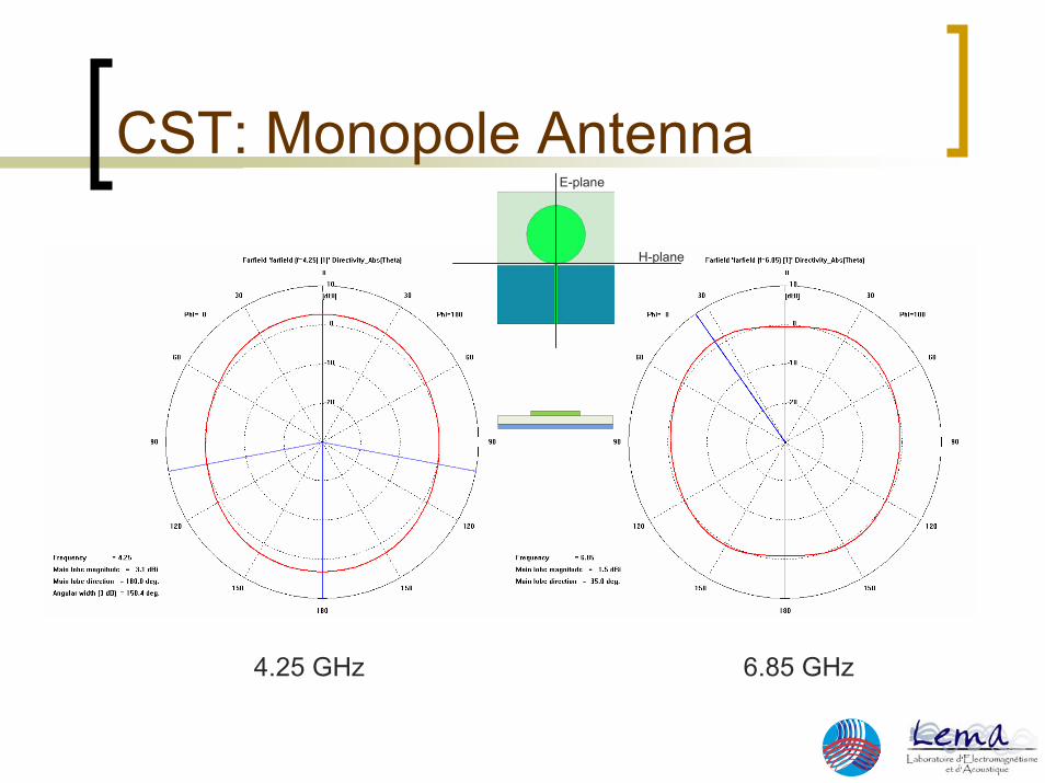
CST: Monopole Antenna
4.25 GHz 6.85 GHz
H-plane
E-plane
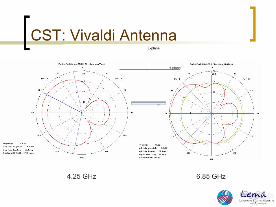
CST: Vivaldi Antenna
4.25 GHz 6.85 GHz
H-plane
E-plane
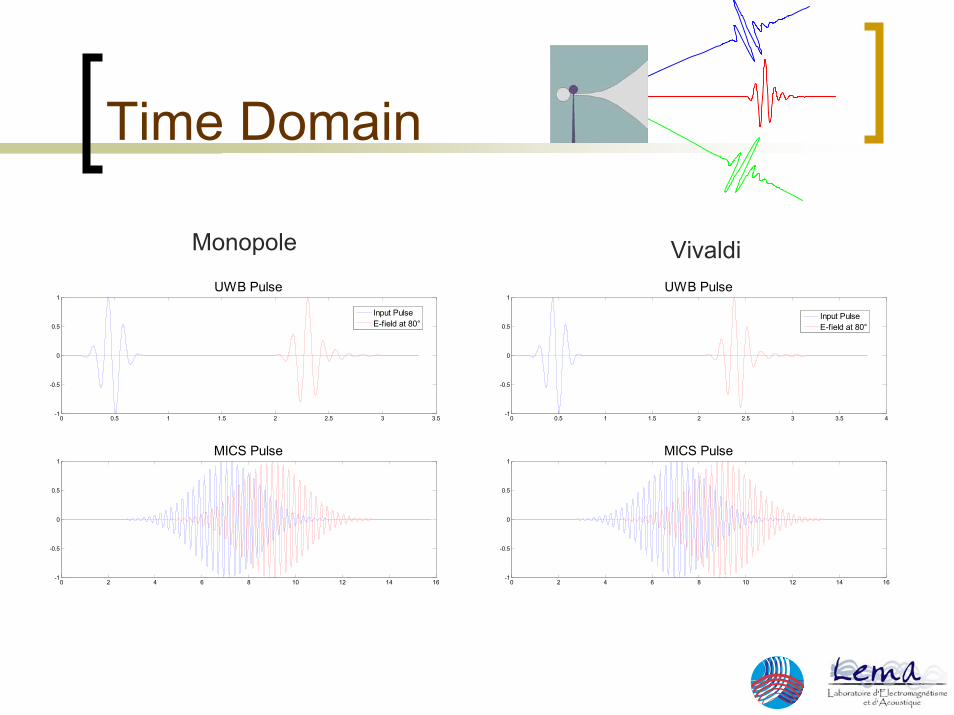
0 0.5 1 1.5 2 2.5 3 3.5 4-1
-0.5
0
0.5
1UWB Pulse
0 2 4 6 8 10 12 14 16-1
-0.5
0
0.5
1MICS Pulse
Input PulseE-field at 80°
Time Domain
0 0.5 1 1.5 2 2.5 3 3.5-1
-0.5
0
0.5
1UWB Pulse
0 2 4 6 8 10 12 14 16-1
-0.5
0
0.5
1MICS Pulse
Input PulseE-field at 80°
Monopole Vivaldi
Time Domain
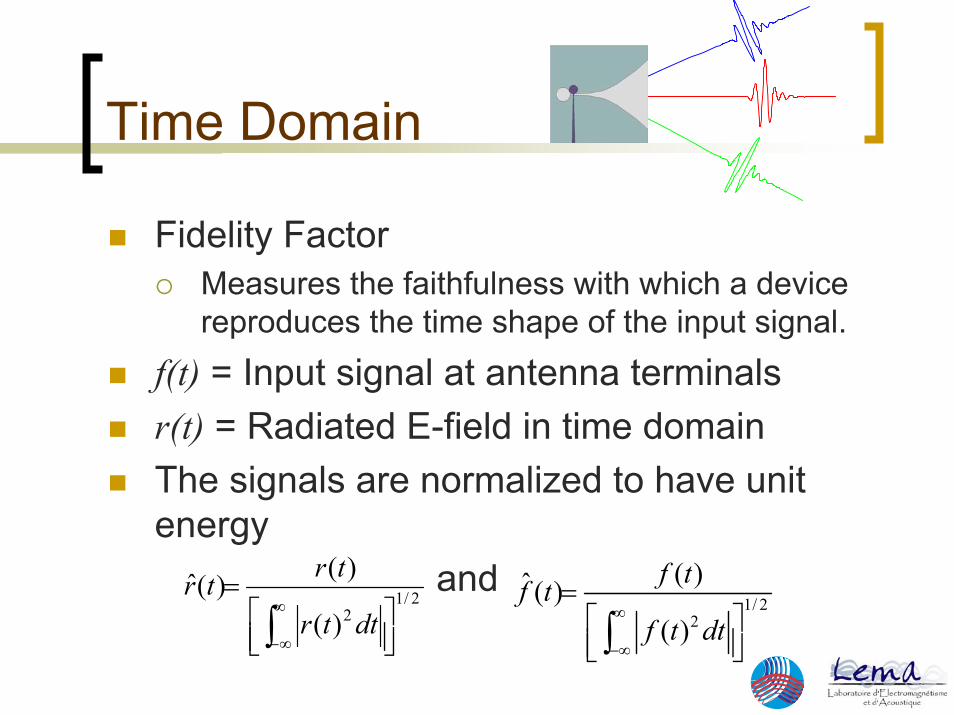
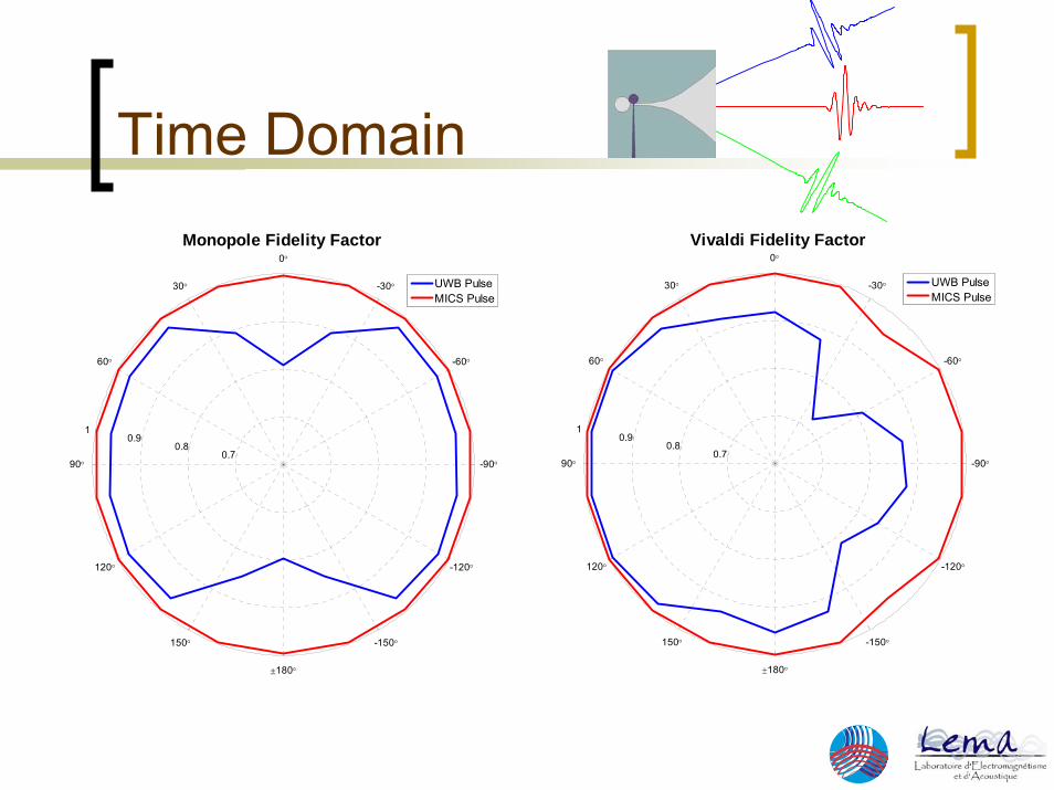
Fidelity FactorMeasures the faithfulness with which a device reproduces the time shape of the input signal.
f(t) = Input signal at antenna terminalsr(t) = Radiated E-field in time domainThe signals are normalized to have unit energy
and2/1
2)(
)()(ˆ
⎥⎦⎤
⎢⎣⎡
=
∫∞
∞−dttr
trtr1/ 2
2
( )ˆ ( )( )
f tf tf t dt
∞
−∞
=⎡ ⎤⎢ ⎥⎣ ⎦∫
Time Domain
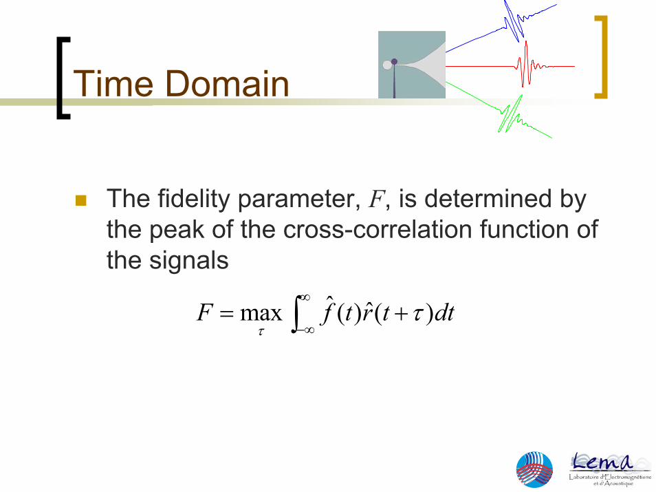
The fidelity parameter, F, is determined by the peak of the cross-correlation function of the signals
ˆ ˆmax ( ) ( )F f t r t dtτ
τ∞
−∞= +∫
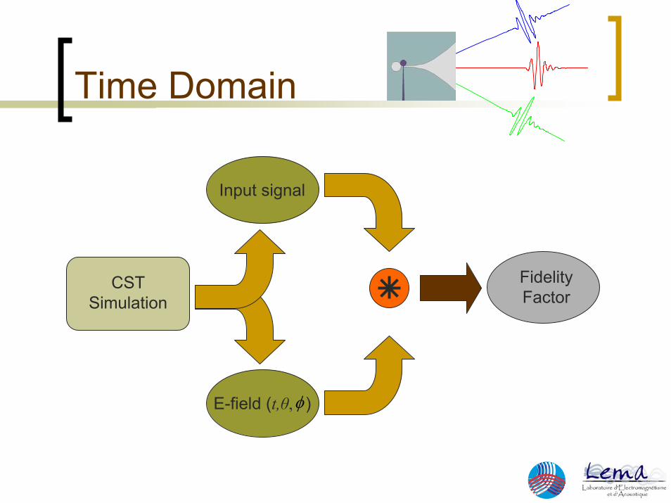
Time Domain
CST Simulation
E-field (t,θ, )
Input signal
Fidelity Factor
φ
Time Domain
0°
30°
60°
90°
120°
150°
±180°
-150°
-120°
-90°
-60°
-30°
0.70.8
0.91
Vivaldi Fidelity Factor
UWB PulseMICS Pulse
0°
30°
60°
90°
120°
150°
±180°
-150°
-120°
-90°
-60°
-30°
0.70.8
0.91
Monopole Fidelity Factor
UWB PulseMICS Pulse
Outline
UWB Antenna AnalysisFrequency DomainTime Domain
Measurement TechniquesPeak and Average Power MeasurementsSpectrum Analyzer Settings
Fourier SeriesFourier Transform
UWB Measurements
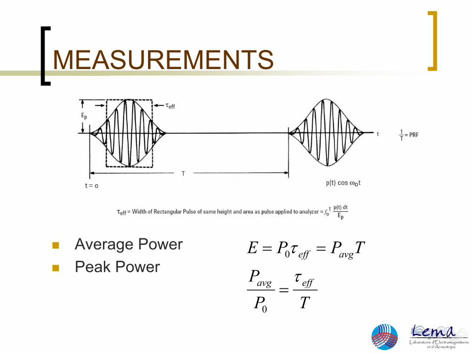
MEASUREMENTS
Average PowerPeak Power
TPP
TPPE
effavg
avgeff
τ
τ
=
==
0
0
MEASUREMENTS
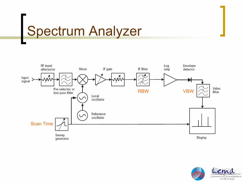
Spectrum Analyzer
RBW VBW
Scan Time
Spectrum Analyzer
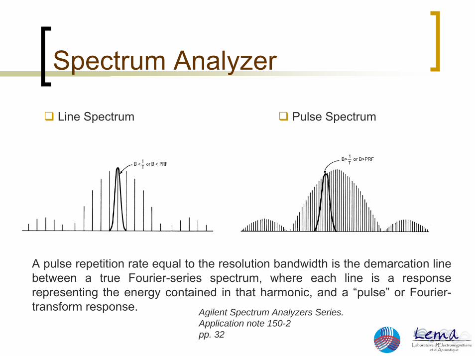
Line Spectrum Pulse Spectrum
A pulse repetition rate equal to the resolution bandwidth is the demarcation line between a true Fourier-series spectrum, where each line is a response representing the energy contained in that harmonic, and a “pulse” or Fourier-transform response. Agilent Spectrum Analyzers Series.
Application note 150-2pp. 32
1B> or B>PRFT
Line Spectrum
Line Spectrum
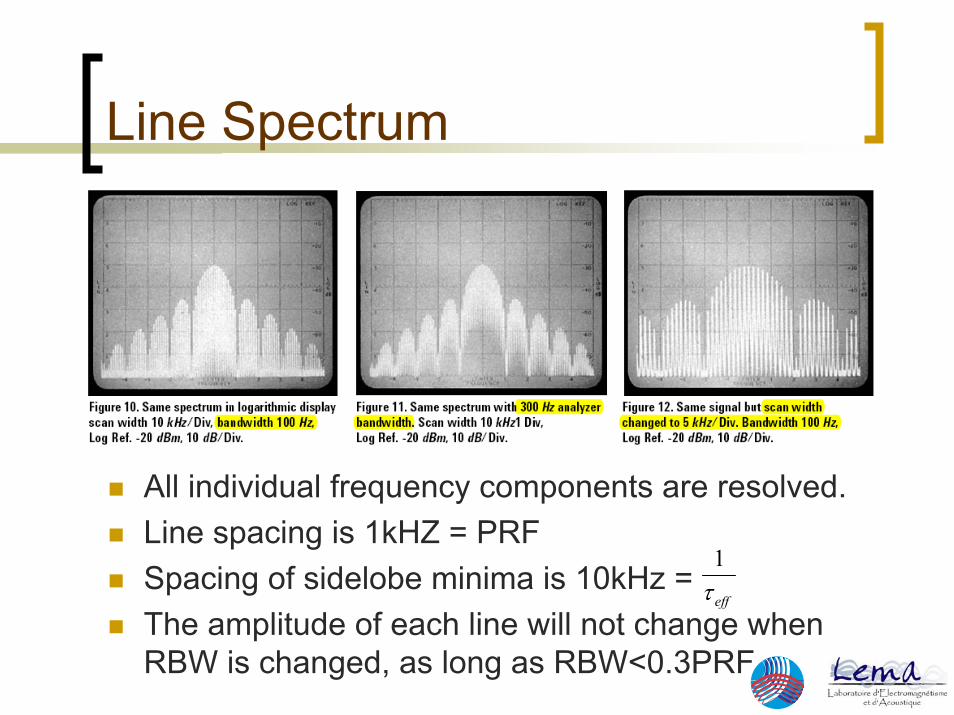
All individual frequency components are resolved.Line spacing is 1kHZ = PRFSpacing of sidelobe minima is 10kHz = The amplitude of each line will not change when RBW is changed, as long as RBW<0.3PRF
1
effτ
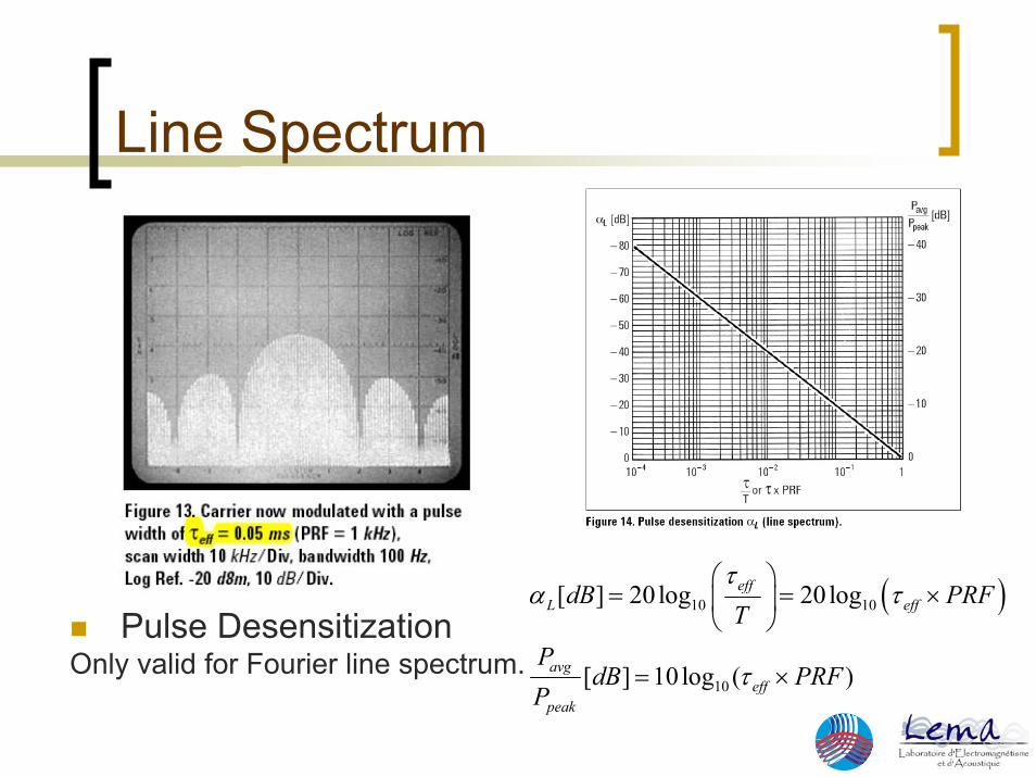
Line Spectrum
Pulse DesensitizationOnly valid for Fourier line spectrum.
( )10 10
10
[ ] 20log 20log
[ ] 10log ( )
τα τ
τ
⎛ ⎞= = ×⎜ ⎟
⎝ ⎠
= ×
effL eff
avgeff
peak
dB PRFT
PdB PRF
P
Pulse Spectrum
It’s a combination of time and frequency display.
The lines that form the envelope are pulse lines in time domain.
Each line is displayed when a pulse occurs.
Frequency domain display of the spectrum envelope.
The amplitude of the envelope increase linearly as RBW increases. (As long as RBW < 0.2/ τeff).
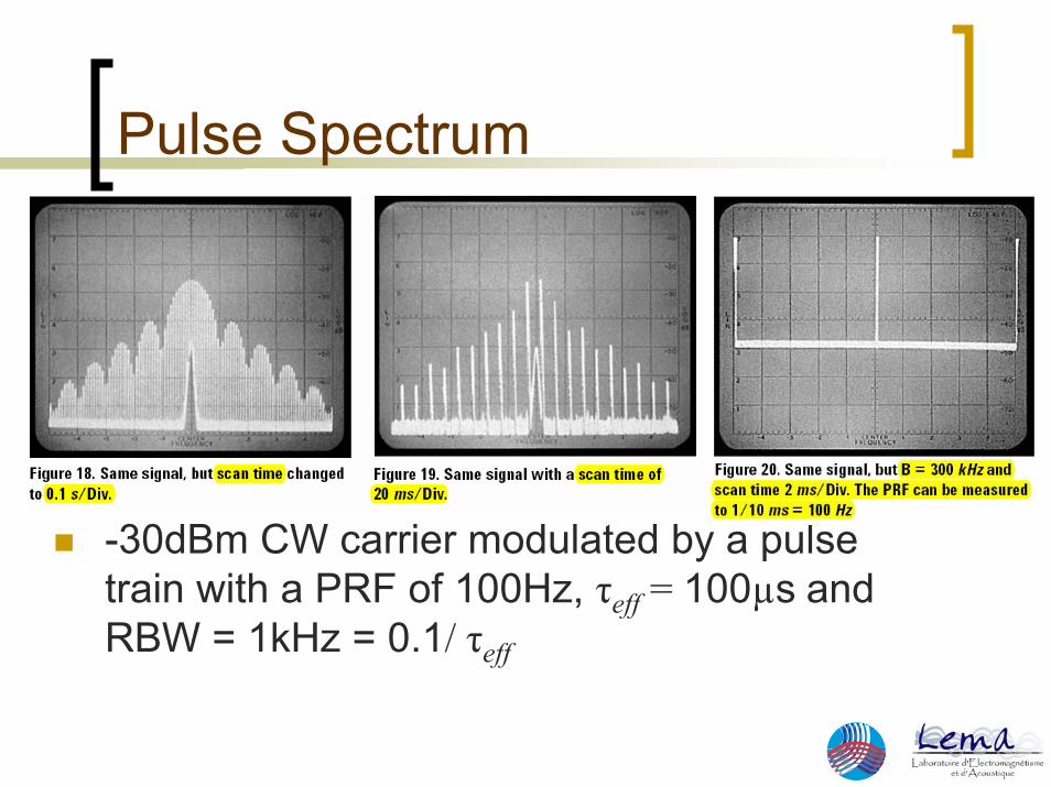
Pulse Spectrum
-30dBm CW carrier modulated by a pulse train with a PRF of 100Hz, τeff = 100µs and RBW = 1kHz = 0.1/ τeff
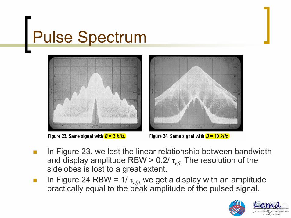
Pulse Spectrum
In Figure 23, we lost the linear relationship between bandwidth and display amplitude RBW > 0.2/ τeff . The resolution of the sidelobes is lost to a great extent.In Figure 24 RBW = 1/ τeff, we get a display with an amplitude practically equal to the peak amplitude of the pulsed signal.
Pulse Spectrum
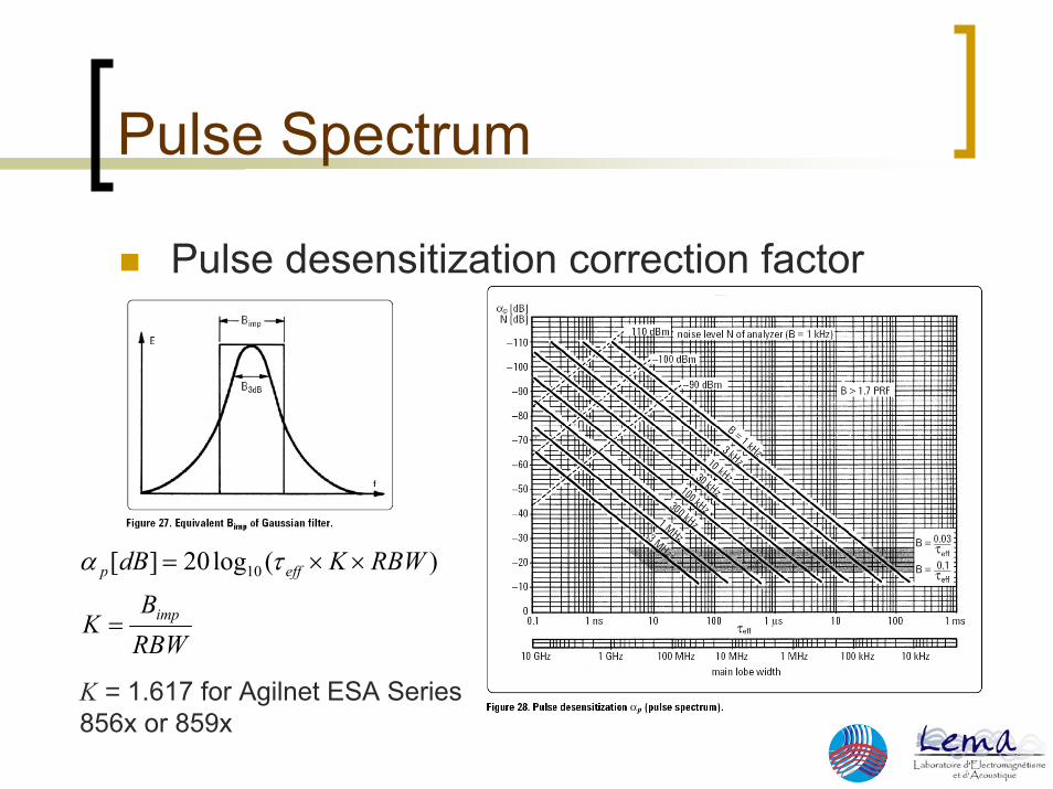
Pulse desensitization correction factor
RBWB
K
RBWKdB
imp
effp
=
××= )(log20][ 10 τα
K = 1.617 for Agilnet ESA Series 856x or 859x
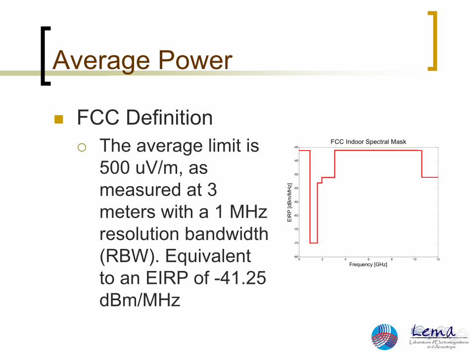
Average Power
FCC DefinitionThe average limit is 500 uV/m, as measured at 3 meters with a 1 MHz resolution bandwidth (RBW). Equivalent to an EIRP of -41.25 dBm/MHz
0 2 4 6 8 10 12-80
-75
-70
-65
-60
-55
-50
-45
-40FCC Indoor Spectral Mask
EIR
P [d
Bm
/MH
z]
Frequency [GHz]
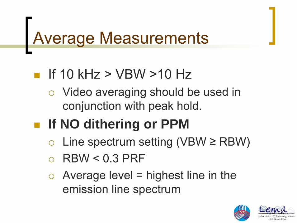
Average Measurements
If 10 kHz > VBW >10 HzVideo averaging should be used in conjunction with peak hold.
If NO dithering or PPMLine spectrum setting (VBW ≥ RBW)RBW < 0.3 PRFAverage level = highest line in the emission line spectrum
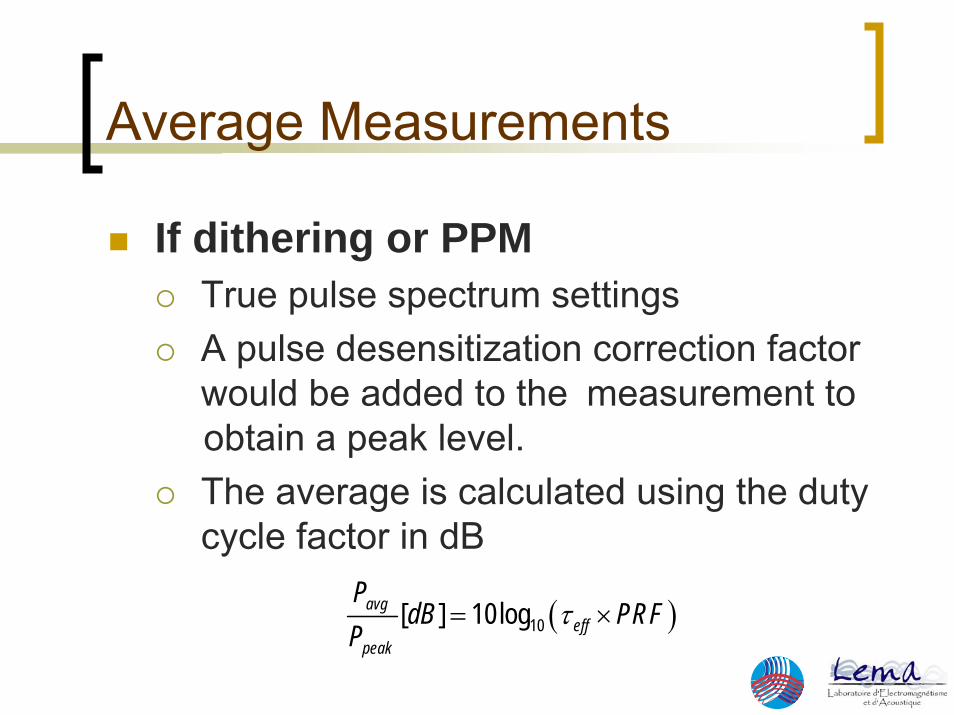
Average Measurements
If dithering or PPMTrue pulse spectrum settingsA pulse desensitization correction factor would be added to the measurement to obtain a peak level.The average is calculated using the duty cycle factor in dB
( )10[ ] 10logavgeff
peak
PdB PRF
Pτ= ×
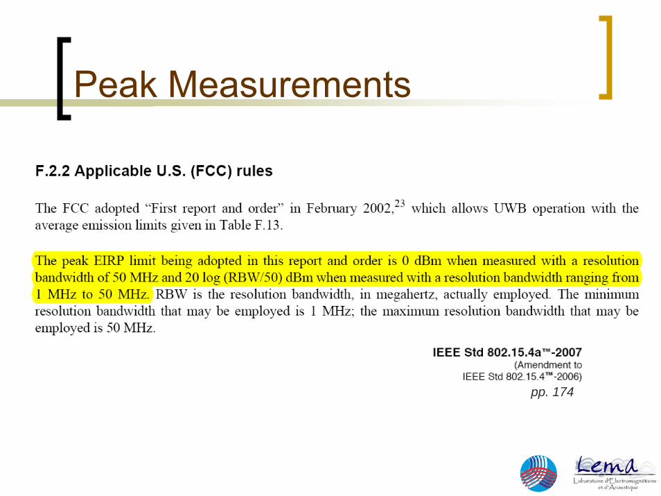
Peak Measurements
pp. 174
Peak Measurements
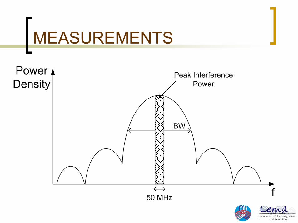
Peak level when measured over a bandwidth of 50 MHz
50MHz → widest victim receiver that is likely to be encountered.
Peak measurements based on a 50 MHz (resolution) bandwidth may not be feasible. The widest available RBW that can be employed for peak measurements is 3 MHz.
Peak Measurements
Peak Measurements
Peak emission level of 0 dBm/50 MHz = 58mV/m at 3 meters is adopted.Equivalent to:
A peak EIRP of -24.44 dBm/3 MHzPeak field strength of 3.46 mV/m at 3 meters with a 3 MHz RBW.
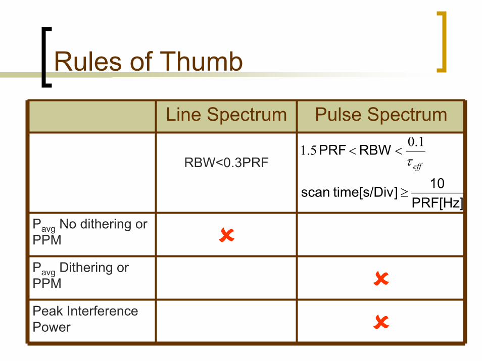
Rules of Thumb
Line Spectrum Pulse Spectrum
RBW<0.3PRF
Pavg No dithering or PPM
Pavg Dithering or PPM
Peak Interference Power
PRF[Hz]10]time[s/Div scan
RBWPRF
≥
<<effτ1.05.1

QUESTIONS?