Embed Size (px)
Citation preview

Anti-Cycling Methods for Linear Programming
Xinyi LuoMathematics Honors Thesis
Advisor: Philip GillUniversity of California, San Diego
June 6th, 2018
Abstract
A linear program (or a linear programming problem, or an LP) is an op-timization problem that involves minimizing or maximizing a linear functionsubject to linear constraints. Linear programming plays a fundamental role notonly in optimization, but also in economics, strategic planning, analysis of al-gorithms, combinatorial problems, cryptography, and data compression. Whenlinear programs are formulated in so-called standard form the set of variablessatisfying the linear constraints (the feasible set) is a convex polytope. If thispolytope is bounded and non-empty, then a solution of the linear program mustlie at a vertex. The simplex method for linear programming moves from onevertex to another until an optimal vertex is found. Almost all practical linearprograms are degenerate, i.e., there are vertices that lie at the intersection ofa set of linearly dependent constraints. The conventional simplex method cancycle at a degenerate vertex, which means that the iterations can be repeatedinfinitely without changing the variables. In the first part of this thesis, wediscuss the e↵ects of degeneracy and investigate several non-simplex methodsthat avoid cycling by solving a linear least-squares subproblem at each itera-tion. In the second part, we propose a new active-set method based on addinga penalty term to the linear objective function. Numerical results indicate thatthe proposed method is computationally e�cient.
1

2 CONTENTS
Contents
1. Introduction 4
2. Notation, Definitions and Theorems 52.1 Notation . . . . . . . . . . . . . . . . . . . . . . . . . . . . . . . . . 52.2 Definitions . . . . . . . . . . . . . . . . . . . . . . . . . . . . . . . . 52.3 Theorems and Lemmas . . . . . . . . . . . . . . . . . . . . . . . . . 6
3. Primal-Dual Non-Negative Least Squares 63.1 Solving the Linear Program . . . . . . . . . . . . . . . . . . . . . . . 6
3.1.1 Finding a feasible ascent direction . . . . . . . . . . . . . . . 63.1.2 The PDNNLS algorithm . . . . . . . . . . . . . . . . . . . . 83.1.3 Finding a feasible point . . . . . . . . . . . . . . . . . . . . . 8
3.2 Solving the NNLS Sub-problem . . . . . . . . . . . . . . . . . . . . . 93.2.1 Optimality conditions for NNLS . . . . . . . . . . . . . . . . 93.2.2 The Lawson and Hanson method . . . . . . . . . . . . . . . . 103.2.3 Fast NNLS algorithm . . . . . . . . . . . . . . . . . . . . . . 12
4. Mixed Constraints 124.1 Solving the Mixed-Constraint LP . . . . . . . . . . . . . . . . . . . . 13
4.1.1 Optimality conditions . . . . . . . . . . . . . . . . . . . . . . 134.1.2 Finding a descent direction . . . . . . . . . . . . . . . . . . . 144.1.3 The algorithm . . . . . . . . . . . . . . . . . . . . . . . . . . 154.1.4 Finding a feasible point . . . . . . . . . . . . . . . . . . . . . 16
4.2 Solving Bounded Least Square Problems . . . . . . . . . . . . . . . 164.2.1 Solving BLS using the singular-value decomposition . . . . . 164.2.2 Dax’s method for BLS . . . . . . . . . . . . . . . . . . . . . . 19
5. A Primal-Dual Active Set Method for Regularized LP 205.1 Formulation of the Primal and Dual Problems . . . . . . . . . . . . 215.2 Optimality Conditions and the KKT Equations . . . . . . . . . . . . 215.3 The Primal Active-Set Method . . . . . . . . . . . . . . . . . . . . . 275.4 The Dual Active-Set Method . . . . . . . . . . . . . . . . . . . . . . 305.5 Degeneracy . . . . . . . . . . . . . . . . . . . . . . . . . . . . . . . . 325.6 Combining Primal and Dual Active-set Methods . . . . . . . . . . . 32
5.6.1 Shifting the primal problem . . . . . . . . . . . . . . . . . . . 335.6.2 Shifting the dual problem . . . . . . . . . . . . . . . . . . . . 33
6. Matrix Factorizations and Updating 356.1 Using the QR Decomposition for Solving Least-Squares Problems . 36
6.1.1 Calculating a null-space descent direction . . . . . . . . . . . 366.1.2 Calculating the projection matrix . . . . . . . . . . . . . . . 366.1.3 Solving the KKT equations . . . . . . . . . . . . . . . . . . . 37
6.2 Updating the QR Factorization . . . . . . . . . . . . . . . . . . . . . 376.3 Modification after a Rank-one Change . . . . . . . . . . . . . . . . . 38

3
6.4 Adjoining and Deleting a Column . . . . . . . . . . . . . . . . . . . 396.4.1 Adjoining a column . . . . . . . . . . . . . . . . . . . . . . . 396.4.2 Removing a column . . . . . . . . . . . . . . . . . . . . . . . 40
6.5 Adjoining and Deleting a Row . . . . . . . . . . . . . . . . . . . . . 416.5.1 Adjoining a row . . . . . . . . . . . . . . . . . . . . . . . . . 416.5.2 Deleting a row . . . . . . . . . . . . . . . . . . . . . . . . . . 41
6.6 Other Factorization Methods . . . . . . . . . . . . . . . . . . . . . . 426.6.1 The symmetric indefinite factorization . . . . . . . . . . . . . 42
7. Numerical Examples 437.1 Highly Degenerate Problems . . . . . . . . . . . . . . . . . . . . . . 44
7.1.1 Test problems . . . . . . . . . . . . . . . . . . . . . . . . . . 447.1.2 Computational results . . . . . . . . . . . . . . . . . . . . . . 44
7.2 Cycling Problems . . . . . . . . . . . . . . . . . . . . . . . . . . . . 457.2.1 Test problems . . . . . . . . . . . . . . . . . . . . . . . . . . 457.2.2 Computational results . . . . . . . . . . . . . . . . . . . . . . 45
8. Summary and Conclusion 46
References 47
4 Anti-Cycling Methods for Linear Programming
1. Introduction
In this paper we consider methods for the solution of the linear programming (LP)problem in standard form, i.e.,
(LP)minimize
x
cTx
subject to Ax = b x � 0,
where A is a constant m⇥ n matrix, and b and c are constant vectors with m andn components, respectively. The set of variables satisfying the linear constraints of(LP) (the feasible set) is a convex polytope. If this polytope is bounded and non-empty, then a solution of the linear program (LP) must lie at a vertex of the feasibleset. A vertex is characterized by a non-negative basic solution of the equationsAx = b that is calculated by solving an m⇥m system of equations BxB = b, wherethe columns of B are a subset of the columns of A. The set of indices of the columnsof A used to define B is known as a basis. The variables associated with the columnsof B are known as the basic variables. The variables with indices that are not inthe basis are known as the nonbasic variables.
The simplex method was the first method to be proposed for solving a linearprogram (see, e.g., [5]). The simplex method moves repeatedly from one vertex toan adjacent vertex until an optimal vertex is found. Each change of vertex involvesmoving a variable from the nonbasic set to the basic set and vice-versa. Each itera-tion involves solving two systems of linear equations of order m. Almost all practicallinear programs are degenerate, i.e., there are vertices that lie at the intersection ofa set of linearly dependent constraints. Unfortunately, the conventional simplexmethod can cycle at a degenerate vertex, which means that the iterations can berepeated infinitely without changing the variables. A crucial decision associatedwith the simplex method is the choice of which variable should enter the basis ateach iteration. This choice is determined by so-called pivot rules. A good choiceof pivot can prevent cycling on degenerate problems and enhance the speed of themethod. The “Dantzig rule” [5] is the earliest and simplest pivot rule and choosesthe variable with the most negative reduced cost to enter the basis. Unfortunately,the simplex method implemented with the Dantzig rule can cycle. Bland’s pivotrule [3] defines a choice of entering and leaving variable that precludes the possibil-ity of cycling. However, an implementation of the simplex method with Bland’s ruleusually requires substantially more iterations to solve an LP than an implementa-tion based on the Dantzig rule. One variation of Dantzig rule is the steepest-edgealgorithm [7,16]. It chooses an entering index with the largest rate of change in theobjective. The steepest-edge simplex method can be e�cient in terms of reducingthe number of simplex iterations, but can also cause the simplex method to cycle.
In the 71 years since the simplex method was first proposed, two other typesof method for solving a linear program have been proposed. The first of these isthe interior-point method. Interest in these methods was initiated by Karmarkar’sannouncement [17] in 1984 of a polynomial-time linear programming method thatwas 50 times faster than the simplex method. Amid the subsequent flurry of interestin Karmarkar’s method, it was shown in 1985 [11] that there is a formal equivalence

2. Notation, Definitions and Theorems 5
between Karmarkar’s method and the classical logarithmic barrier method appliedto linear programming. This resulted in many long-discarded barrier methods beingproposed as polynomial-time algorithms for linear programming. One of the mainfeatures of an interior method is that every iterate lies in the strict interior of thefeasible set, which implies that there is no basis defined. In the past thirty years,many e�cient implementations of the interior-point method and its variants havebeen developed [18, 20–22]. Extensive numerical results indicate that robust ande�cient implementations of the interior-point method can solve many large-scaleLP problems. As all the iterates lie inside the feasible set, it is not possible for aninterior-point method to cycle.
This paper will focus on the second alternative to the simplex method, whichis an active-set method that does not necessarily move from vertex to vertex. Thismethod is similar to the simplex method in the sense that it uses a basis withindependent columns. However, unlike the simplex method, the basis matrix doesnot have to be square.
Instead of solving (LP) directly by using an active-set method, we considermethods based on solving a non-negative least-squares subproblem of the form
(NNLS)minimize
x
kABx� bk2
subject to x � 0,
where k ·k denotes the two-norm of a vector, and AB denotes a working basis matrix.
2. Notation, Definitions and Theorems
2.1. Notation
Unless explicitly indicated otherwise, k·k denotes the vector two-norm or its inducedmatrix norm. Given vectors a and b with the same dimension, min(a, b) is a vectorwith components min(a
i
, bI). The vectors e and ej
denote, respectively, the columnvector of ones and the jth column of the identity matrix I. The dimensions of e,ei
and I are defined by the context. Given vectors x and y, the column vectorconsisting of the components of x augmented by the components of y is denoted by(x, y).
2.2. Definitions
Definition 2.1. The primal and dual linear programs associated with problem (LP)are
(P) minimizex2Rn
cTx subject to Ax = b, x � 0,
and
(D) maximizey2Rm
bTy subject to ATy c,
where (D) is the dual of problem (P).

6 Anti-Cycling Methods for Linear Programming
Definition 2.2. (Feasible direction) Let y be a feasible point for the linear in-equality constraints ATy c. A dual feasible direction at y is a vector p satisfying
p 6= 0 and AT(y + ↵p) c for some ↵ > 0.
2.3. Theorems and Lemmas
Theorem 2.1. (Farkas’ Lemma) Let A 2 Rm⇥n and b 2 Rm. Then exactly oneof the following two systems is feasible:
1. {x : Ax = b, x � 0},
2. {y : AT y 0, bT y > 0}.
Theorem 2.2. (Dual active-set optimality conditions for an LP)A point x⇤ is a solution of (LP) if and only if Ax⇤ = b, ABx⇤B = b with x⇤B � 0, andthere exists a y⇤ such that ATy⇤ c, where AB is the active-constraint matrix at y⇤.
3. Primal-Dual Non-Negative Least Squares
In this section we present a modification of the method of Barnes et al. [1] tosolve the linear program (LP). The primal-dual non-negative least-squares method(PDNNLS) is based on solving the dual problem (D) instead of the primal problem(P). A strict feasible ascent direction for the dual is found by using the residualvector from the solution of a non-negative least squares sub-problem (NNLS). Asuitable step along this direction will increase the objective function of (D) at eachiteration.
The main algorithm PDNNLS is described in section 3.1.2 and its correspondingformulation of phase 1 problem is described in Section 3.1.3. In Section 3.2 wepresent methods for solving (NNLS) subproblem that can be used in PDNNLS.
3.1. Solving the Linear Program
3.1.1. Finding a feasible ascent direction
Theorem 3.1. Let x⇤ be the solution of the problem
(NNLS) minimizex2Rt
1
2
kABx� bk2 subject to x � 0,
where AB is the submatrix corresponding to B, and |B| = t. Let �y = b�ABx⇤. If�y 6= 0 then �y is a feasible ascent direction for (D), i.e. bT�y > 0.
Proof. The Lagrangian of (NNLS) with y as the multiplier is given by
L(x, y) = 1
2
(ABx� b)T(ABx� b)� yTx.
3. Primal-Dual Non-Negative Least Squares 7
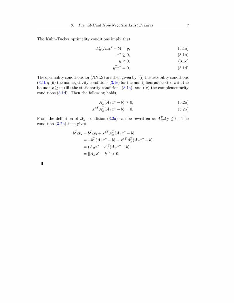
The Kuhn-Tucker optimality conditions imply that
AT
B(ABx⇤ � b) = y, (3.1a)
x⇤ � 0, (3.1b)
y � 0, (3.1c)
yTx⇤ = 0. (3.1d)
The optimality conditions for (NNLS) are then given by: (i) the feasibility conditions(3.1b); (ii) the nonnegativity conditions (3.1c) for the multipliers associated with thebounds x � 0; (iii) the stationarity conditions (3.1a); and (iv) the complementarityconditions.(3.1d). Then the following holds,
AT
B(ABx⇤ � b) � 0, (3.2a)
x⇤TAT
B(ABx⇤ � b) = 0. (3.2b)
From the definition of �y, condition (3.2a) can be rewritten as AT
B�y 0. Thecondition (3.2b) then gives
bT�y = bT�y + x⇤TAT
B(ABx⇤ � b)
= �bT (ABx⇤ � b) + x⇤TAT
B(ABx⇤ � b)
= (ABx⇤ � b)T(ABx
⇤ � b)
= kABx⇤ � bk2 > 0.

8 Anti-Cycling Methods for Linear Programming
3.1.2. The PDNNLS algorithm
The motivation for the algorithm PDNNLS is to solve problem (NNLS) at eachiteration and use �y = b� ABx⇤ as an ascent direction for the dual problem. Thealgorithm is described below.
Algorithm 1 Primal-Dual Non-Negative Least Squares (PDNNLS).
1: input A, b, c, and a dual feasible point y;2: while not convergent do3: Let B be the active set for AT y c, so that AT
By = cB;4: Solve (NNLS) for x⇤;5: if ABx⇤ = b then6: stop; [(x⇤, y⇤) is optimal]7: else8: �y b�ABx⇤;9: end if
10: if AT
N�y 0 then11: stop; [The dual is unbounded below]12: else13: ↵ min
i:i2N ,a
Ti �y>0
ci�a
Ti y
a
Ti �y
;
14: end if15: y y + ↵�y;16: end while17: return x, y;
3.1.3. Finding a feasible point
If c � 0, then y0
= 0 is feasible for the constraints ATy c and y0
can be usedto initialize Algorithm PDNNLS. Otherwise, an initial dual feasible point can becomputed by solving the phase 1 linear program:
minimizey2Rm
,✓2R✓
subject to ATy + ✓e c, ✓ 0.
An initial feasible point for this LP is given by (y0
, ✓0
), where y0
= 0 and ✓0
= mini
ci
.Consider the quantities A 2 R(m+1)⇥(n+1), b 2 Rm+1, c 2 Rn+1 and initial dualfeasible point y
0
such that
A =
✓
A 0eT 1
◆
, b =
0
B
B
B
@
0...01
1
C
C
C
A
, c =
✓
c0
◆
, y0
=
✓
y0
✓0
◆
.
Use A, b, c, and y0
as input for (PDNNLS). If the associated dual (D) is feasible,then the phase 1 problem will have an optimal solution with zero objective value

3. Primal-Dual Non-Negative Least Squares 9
and final iterate y = (y1
, 0). If the optimal phase 1 objective is nonzero the dual isinfeasible and the primal (P) is unbounded. If phase 1 terminates with a feasibley1
, the original coe�cient matrix A, cost vector c, and the bound constraint vectorb can be used as input for a second phase to solve using (PDNNLS).
3.2. Solving the NNLS Sub-problem
Over the years, various methods have been developed for solving NNLS. Generally,approaches can be divided into three broad categories. The first includes iterativemethods such as gradient projection methods and barrier methods. The second cat-egory includes methods based on transforming NNLS into a least-distance problemthat is solved as a linear inequality constrained least-squares problem. The thirdcategory includes other active-set methods that do not transform NNLS into anequivalent least-distance problem.
In this section we focus on active-set methods. Specifically, we present theclassical Lawson and Hanson algorithm and its improved version known as the fastnon-negative least squares method (FNNLS).
3.2.1. Optimality conditions for NNLS
The classical NNLS algorithm was proposed by Lawson and Hanson [19] in 1974 forsolving the following problem
minimizex2Rn
kAx� bk subject to Dx � f,
where A 2 Rm⇥n and b 2 Rm. This problem is equivalent to NNLS if D = I andf = 0. Consider the problem
minimizex2Rn
kAx� bk subject to x � 0.
which is equivalent to the problem
(NNLS) minimizex2Rn
1
2
kAx� bk2 subject to x � 0.
Proposition 3.1. (Kuhn-Tucker Conditions) A vector x 2 Rn is an optimalsolution for problem (NNLS) if and only if there exists a y 2 Rn satisfying
AT(Ax� b) = y, (3.3a)
x � 0, (3.3b)
y � 0, (3.3c)
xTy = 0. (3.3d)
Proof. The Lagrangian for (NNLS) is
L(x, y) = (Ax� b)T(Ax� b)� yTx.

10 Anti-Cycling Methods for Linear Programming
Stationary of the Lagrangian with respect to x implies that
AT(Ax� b)� y = 0. (3.4)
The optimality conditions for (NNLS) are then given by: (i) the feasibility conditions(3.3b); (ii) the nonnegativity conditions (3.3c) for the multipliers associated with thebounds x � 0; (iii) the stationarity conditions (3.3a); and (iv) the complementarityconditions.(3.3d).
3.2.2. The Lawson and Hanson method
The NNLS algorithm is described below. The inputs include a matrix A 2 Rm⇥n
and a vector b 2 Rm. The dual vector y is calculated and the corresponding workingset B and non-working set N are defined and modified each iteration. The workingset is changed as follows: in the main loop, the algorithm calculates the dual vectory, selects the most negative index of the dual vector and adds it to B. In the innerloop, the algorithm tries to satisfy the primal feasibility condition (3.3b) by findingan vector z such that its subvector zB corresponding to B solves the least-squareproblem while its subvector zN corresponding to N will always be held at value zero.Inside the primal feasibility loop, xN will always be zeros while xB will be free totake values other than zero. If there is any variable x
i
< 0, i 2 B, the algorithmwill either take a step to change it to a positive value, or set the variable to 0 andmove it to N .
Algorithm 2 Non-Negative Least Squares.
B ;; N {1, . . . , n}; x 0; [Fix all variables on their bounds]y AT(Ax� b);while N 6= ; and 9i : y
i
< 0 dol argmin
i2N; y
i
;
B B [ l, N N \ l;zN 0 and find zB by solving minimize
z2RtkABz � bk;
while 9i 2 B : zi
< 0 dok argmin
i2B,zi0
xi
/(xi
� zi
);
↵ xk
/(xk
� zk
); [Compute the maximum feasible step]x x+ ↵(z � x);E {i : x
i
= 0};B B \ E ; N N [ E ;zN 0 and find zB by solving minimize
z2RtkABz � bk;
end whilex z;y AT(Ax� b);
end whilereturn x, y;

3. Primal-Dual Non-Negative Least Squares 11
Proposition 3.2. On termination of Algorithm 2, the solution x and the dual vec-tor y satisfy
xi
> 0, yi
= 0, i 2 B,xi
= 0, yi
� 0, i 2 N .
Proof. The resulting solution vector x after the primal feasibility loop will satisfyxN = 0 and xB > 0, where xB is the solution of
minimizex2Rt
kABx� bk.
The vector xB can be written as xB = A†Bb, where A†
B is the Moore-Penrose pseu-doinverse of AB. (If AB has full column rank then A†
B = (AT
BAB)�1AT
Bb). Then
Ax� b = ABxB +ANxN � b = ABA†Bb� b = �(I �ABA
†B)b,
and the subvector of y corresponding to B is
yB = AT
B(Ax� b) = �AT
B(I �ABA†B)b = 0,
because the vector (I �ABA†B)b lies in the null space of AT
B . The termination of themain loop implies that yN � 0, which implies that y � 0.
The NNLS algorithm requires a finite number of iterations to obtain a solu-tion. For the finiteness of NNLS algorithm, we refer readers to [19] for more detail.
However, the significant cost of computing the pseudoinverse A†B in Steps 6 and 13
implies that the method is slow in practice.

12 Anti-Cycling Methods for Linear Programming
3.2.3. Fast NNLS algorithm
Many improved algorithms have been suggested since 1974. Fast NNLS (FNNLS) [4]is an optimized version of the Lawson and Hanson’s algorithm which implementedin the Matlab routine lsqnonneg. It uses precomputed cross-product matrices inthe normal equation formulation and used them repeatedly.
Algorithm 3 Fast non-negative least squares.
Choose x; Compute N = {i : xi
= 0} and B = {i : xi
> 0};repeat
repeatzB = argmin
z
kABz � bk; zN = 0;if min
j2B zj
< 0 thenk argmin
i2B,zi<0
xi
/(xi
� zi
);
↵ xk
/(xk
� zk
); [Compute the maximum feasible step]N N [ {k}, B B \ {k}; [fix x
k
on its bound]x x+ ↵(z � x);
elsex = z;
end ifuntil x = zy AT(Ax� b);ymin
mini2N
yi
; l argmini2N
yi
;
if ymin
< 0 thenB B [ {l}; N N \ {l}; [free x
l
from its bound]end if
until ymin
� 0return x, y;
4. Mixed Constraints
The idea of solving linear programming by solving a least-squares subproblem forthe dual feasibility can be extended to problems with a mixture of equality andinequality constraints. Consider the following problem
minimizex2Rn
cTx
subject to aTi
x = bi
, for i 2 E , aTi
x � bi
, for i 2 I,(4.1)
where E , I are partitions of M = {1, . . . ,m} with E\I = ;. The quantity E denotesthe index set of the equality constraints, and it is assumed that |E| = m
1
. Similarly,I denotes the index set of the inequality constraints, with |I| = m
2
. Also, let Bdenote the indices of a basis. Let A be an m⇥ n matrix with i-th row vector givenby aT
i
. Let AE and AI denote the matrices consisting of rows of A with indices in E

4. Mixed Constraints 13
and I, respectively. Therefore, (4.1) is equivalent to
(PMC
)minimize
x2RncTx
subject to AEx = bE, AIx � bI .
4.1. Solving the Mixed-Constraint LP
4.1.1. Optimality conditions
Proposition 4.1. A vector x 2 Rn is an optimal solution for problem (PMC
) if andonly if there exists a y 2 Rm such that
AEx = bE, (4.2a)
AIx � bI , (4.2b)
ATy = c, (4.2c)
yI � 0, (4.2d)
yTI (AIx� bI) = 0, (4.2e)
where yE, and yI are the vectors of components of the Lagrangian multiplier y as-sociated with E and I, respectively.
The Lagrangian is given by
L(x, y) = cTx� yTE (AEx� bE)� yTI (AIx� bI)
= xT(c�AT
Ey �AT
I yI) + bTEyE + bTI yI
= bTEyE + bTI yI + xT(c�ATy)
= bTy � xT(ATy � c),
which implies that the dual problem is
(DMC
)maximize
y2RmbT y
subject to ATy = c, yI � 0.
From the formulation of (DMC
), the following proposition holds.
Proposition 4.2. Let B denote a working basis. If yi
� 0 for i 2 I \B, and yi
= 0for i 2 N , then y solves problem (D
MC
).
Proof. The complementary slackness conditions (4.2e) are satisfied when aTi
x�bi
=0, for i 2 I \B. The non-negativity of the multipliers associated with the inequalityconstraints (4.2d) requires y
i
� 0 for i 2 I \B. For i 2M\B it holds that aTi
x 6= bi
and yi
must be zero to satisfy the complementarity conditions.
By Proposition 4.2, the mixed constraint problem (4.1) is equivalent to solvingthe bound constrained linear least-squares subproblem
(BLS)minimize
y2RtkAT
B y � ck2
subject to yi
� 0, i 2 I \ B.

14 Anti-Cycling Methods for Linear Programming
If the subvector y⇤B is the optimal solution of problem (BLS) and y⇤N = 0, then y⇤ isthe optimal solution of problem (D
MC
). Otherwise, we find a feasible descent direc-tion for the primal problem (P
MC
) and update the current iterate. An appropriatemethod for solving problem (BLS) is described in Section 4.2.
4.1.2. Finding a descent direction
The method for solving a problem with mixed constraints uses two di↵erent typesof descent direction. Each of these directions is the residual vector at the solutionsof a linear least-squares problem.
A Type-1 descent direction is computed by solving the unconstrained least-squares problem
minimizey2Rt
kAT
By � ck2.
If y⇤ is the optimal solution of this problem, then �x = AT
By⇤ � c is a feasible
descent direction for the primal. For a proof, we refer the reader to [10]. The searchdirection may be regarded as a gradient descent direction in range(AB).
A Type-2 descent direction is found by solving the bound-constrained problem(BLS). To establish that the optimal residual of this problem is a feasible descentdirection, we first state the optimality conditions of (BLS).
Proposition 4.3. A vector y 2 Rt is an optimal solution for problem (BLS) if andonly if there exists a vector � 2 Rn satisfying the following conditions.
yi
� 0, i 2 I \ B, (4.3a)
AB(AT
By � c) = �, (4.3b)
� � 0, (4.3c)
�Ty = 0. (4.3d)
The motivation for finding the feasible descent direction is similar to the ideadescribed in Section 3.1. We use the residual vectors as the search direction. Thefollowing proposition proves that such direction is a feasible descent direction forthe (P
MC
).
Proposition 4.4. Assume that y⇤ solves (BLS) and let r = AT
By⇤ � c. If r = 0,
then x solves the mixed-constraint linear program (4.1). Otherwise, r is a feasibledescent direction for (P
MC
).
Proof. Assume that r = 0. Let p be a feasible direction, i.e., p satisfies aTi
p � 0 fori 2 I \ B and aT
i
p = 0 for i 2 E . Then
cTp = (AT
By⇤)Tp = y⇤T(AT
Bp) =X
i2I\By⇤i
(aTi
p) +X
i2Ey⇤i
(aTi
p) =X
i2I\By⇤i
(aTi
p) � 0.
It follows that every feasible direction is a direction of increase for the objective,which implies that x solves (4.1).

4. Mixed Constraints 15
If r 6= 0, it follows directly from Proposition 4.3 that
ABr = AB(AT
By⇤ � c) = � � 0.
Also, since c = AT
By⇤ � r, and conditions (4.3b) and (4.3d) hold, we have
cTr = (AT
B y⇤ � r)T r = y⇤TABr � krk2 = y⇤T�� krk2 = �krk2 < 0.
This proves the claim.
4.1.3. The algorithm
Algorithm 4 below gives the steps of the algorithm for solving an LP with mixedconstraints. In the main loop, a Type-1 direction is used until the stationarityconditions are satisfied, at which point the inner loop is entered. A Type-2 descentdirection is found in the inner loop. Then the algorithm tests if the problem isunbounded above by checking if the search direction �y satisfies AT
N�y � 0. Thestep size ↵ is then found by calculating the largest step along �y that maintainsthe dual feasibility.
The use of a mixture of Type-1 and Type-2 directions significantly reduces thenumber of times that it is necessary to solve problem (BLS). A similar scheme canbe applied to problem PDNNLS to improve the e�ciency.
Algorithm 4 Mixed Constraints.Input A, b, c, a feasible point x, and Iwhile not converged do
Let B be the active set such that ABx = bB;Solve minimize
y2RtkAT
By � ck2 for y;
if AT
By = c thenif y
i
� 0, i 2 I \ B thenStop; [optimal solution]
end ifCompute y, the solution of
minimizey2Rt
kAT
By � ck2 subject to yi
� 0, i 2 I \ B;
end if�x AT
By � c;if AN�x � 0 then
stop; [unbounded above]else
↵ mini:i2N ,a
Ti �x<0
bi�a
Ti x
a
Ti �x
;
end ifx x+ ↵�x;
end whilereturn x, y;
16 Anti-Cycling Methods for Linear Programming
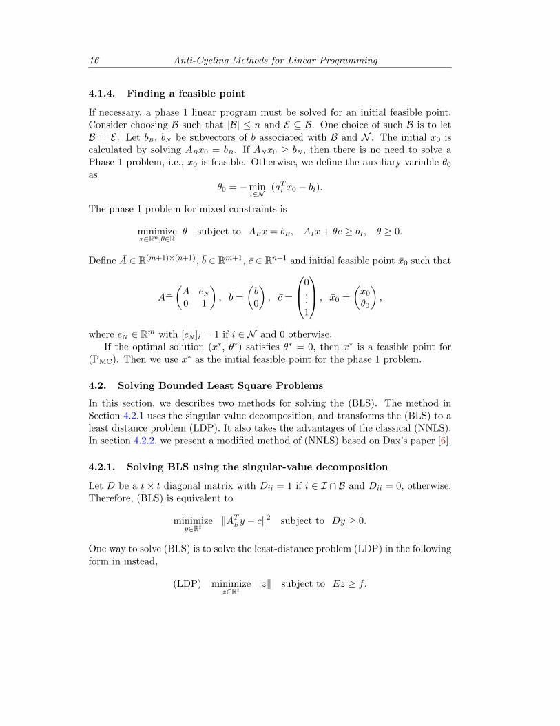
4.1.4. Finding a feasible point
If necessary, a phase 1 linear program must be solved for an initial feasible point.Consider choosing B such that |B| n and E ✓ B. One choice of such B is to letB = E . Let bB, bN be subvectors of b associated with B and N . The initial x
0
iscalculated by solving ABx0 = bB. If ANx0 � bN , then there is no need to solve aPhase 1 problem, i.e., x
0
is feasible. Otherwise, we define the auxiliary variable ✓0
as✓0
= �mini2N
(aTi
x0
� bi
).
The phase 1 problem for mixed constraints is
minimizex2Rn
,✓2R✓ subject to AEx = bE, AIx+ ✓e � bI , ✓ � 0.
Define A 2 R(m+1)⇥(n+1), b 2 Rm+1, c 2 Rn+1 and initial feasible point x0
such that
A=
✓
A eN0 1
◆
, b =
✓
b0
◆
, c =
0
B
@
0...1
1
C
A
, x0
=
✓
x0
✓0
◆
,
where eN 2 Rm with [eN ]i = 1 if i 2 N and 0 otherwise.If the optimal solution (x⇤, ✓⇤) satisfies ✓⇤ = 0, then x⇤ is a feasible point for
(PMC
). Then we use x⇤ as the initial feasible point for the phase 1 problem.
4.2. Solving Bounded Least Square Problems
In this section, we describes two methods for solving the (BLS). The method inSection 4.2.1 uses the singular value decomposition, and transforms the (BLS) to aleast distance problem (LDP). It also takes the advantages of the classical (NNLS).In section 4.2.2, we present a modified method of (NNLS) based on Dax’s paper [6].
4.2.1. Solving BLS using the singular-value decomposition
Let D be a t⇥ t diagonal matrix with Dii
= 1 if i 2 I \ B and Dii
= 0, otherwise.Therefore, (BLS) is equivalent to
minimizey2Rt
kAT
By � ck2 subject to Dy � 0.
One way to solve (BLS) is to solve the least-distance problem (LDP) in the followingform in instead,
(LDP) minimizez2Rt
kzk subject to Ez � f.

4. Mixed Constraints 17
Proposition 4.5. Solving (BLS) is equivalent to solving (LDP).
Proof. Given AB is a matrix of dimension t⇥ n, the singular value decompositiongives
AT
B = bU⌃V T =�
U1
U2
�
✓
⌃0
◆
V T ,
where U and V are orthogonal with dimension n⇥n and t⇥ t respectively. Besides,U1
is of dimension n⇥ t, U2
is of dimension n⇥ (n� t), and ⌃ is a diagonal matrixof dimension t⇥ t. The objective function of (BLS) can be written as
kAT
By � ck2 = kU ⌃V T y � ck2
= k⌃V T y � UT ck2
= k✓
⌃V T y0
◆
�✓
UT
1
cUT
2
c
◆
k2
= k⌃V T y � UT
1
ck2 + kUT
2
ck2
= kzk2 + kUT
2
ck2,
where z = ⌃V T y�UT
1
c. By change of variables, y = V ⌃�1(z+UT
1
c), the constraintof (BLS) becomes
DV ⌃�1z � �DV ⌃�1UT
1
c.
If the constant second term kUT
2
ck2 is omitted, then (LDP) and (BLS) are equivalentfor E = DV ⌃�1 and f = �DV ⌃�1UT
1
c.
The classical NNLS algorithm can be used to compute the solution for (LDP).Instead of computing z directly, we can compute a t vector bu solves the problem
minimizeu2Rt
�
�
�
✓
ET
fT
◆
u� et+1
�
�
�
2 subject to u � 0,
where et+1
is a t+ 1 vector with everywhere zeros except its (t+ 1) entry. Further,
if r =
✓
ET
fT
◆
bu� et+1
, then the following proposition holds.
Proposition 4.6. If zi
= ri
/rt+1
, i = 1, 2, . . . , t, then z solves (LDP).
Proof. The gradient of the objective function 1
2
k✓
ET
fT
◆
u� et+1
k2 at bu is
g =�
E f�
n
✓
ET
fT
◆
bu� et+1
o
=�
E f�
r.
From the KKT condition for the NNLS problem, the complementary slackness con-dition (3.3d) requires gT bu = 0. Then
krk2 = rT r = rTn
✓
ET
fT
◆
bu� et+1
o
= gT bu� rt+1
= �rt+1
> 0.

18 Anti-Cycling Methods for Linear Programming
As zi
= �ri
/rt+1
, for i = 1, 2, . . . , t, we have
r = �rt+1
✓
z�1
◆
.
The dual feasibility condition (3.3c) requires g � 0,
g =�
E f�
r = ��
E f�
✓
z�1
◆
rt+1
= (Ez � f)(�rt+1
) � 0.
The strict inequality �rt+1
> 0 implies that Ez � f , which establishes the feasibilityof constraints.
It remains to show that z is the minimizer. The KKT conditions for (LDP)require that z must be a nonnegative linear combination of rows of E.
z = � 1
rn+1
0
B
@
r1
...rn
1
C
A
= � 1
rn+1
ET
bu =1
krk2ET
bu,
where bu � 0 from the primal feasibility condition of the non-negative least squaresproblem (3.3b). Therefore, z is the solution of Problem (LDP).
By change of variable, i.e., y = V ⌃�1(z + UT
1
c), (LDP) can be solved as well.The BLS algorithm using NNLS is described below.
Algorithm 5 Bounded Least Square-NNLS.Input AB, c;Calculate the economy-size singular value decomposition of AT
B
AT
B = U1
⌃V T ;
E DV ⌃�1; f �DV ⌃�1UT
1
c;Use NNLS to compute bu, the solution of
minimizeu2Rt
�
�
�
�
✓
ET
fT
◆
u� et+1
�
�
�
�
2
subject to u � 0;
r ✓
ET
fT
◆
bu� et+1
;
if r = 0 thenstop; [Ez � f is not compatible]
elsezi
�ri
/rt+1
, i = 1, . . . , t;end ify V ⌃�1(z + UT
1
c);return y;

4. Mixed Constraints 19
This algorithm performs well for low dimensional problems. However, since com-puting the singular value decomposition involves approximately m2n+ n3 floating-point operations for a matrix of dimension m⇥ n, it is not e�cient to compute thesingular-value decomposition from AT
B directly. Instead, we use the economy-sizeQR factorization in the outer loop if n� t and compute the singular value decom-position of the square upper-triangular matrix R. This gives the decomposition
R = U⌃V T ,
which implies that AT
B can be written as
AT
B = Q1
R = Q1
U⌃V T = U1
⌃V T , with U1
= Q1
U .
The singular-value decomposition of R requires 2t3 floating-point operations.
4.2.2. Dax’s method for BLS
Without loss of generality, consider solving the (BLS) in the following form
(BLS)minimize
x2RnkAx� bk2
subject to xi
� 0, i 2 I,
where A 2 Rm⇥n and I ⇢ {1, 2, . . . , n}. To solve the mixed constraints problemsusing the following algorithm, simply substitute A, x, and b with AT
B , y and crespectively.
From Proposition 4.3 and using an appropriate substitution, the following resultholds.
Proposition 4.7. If x is a feasible point for (BLS) and the following equations aresatisfied
yi
= 0, if i 2 E ,yi
= 0, if i 2 I \ B, xi
> 0,
yi
> 0, if i 2 I \ B, xi
= 0,
then x is the optimal solution for (BLS).
Dax’s method is given in Algorithm 6 below. The method performs well whenthere is no degeneracy. However, if a problem is degenerate, a large number ofiterations may be required to solve the bounded least squares problem.

20 Anti-Cycling Methods for Linear Programming
Algorithm 6 Bounded least squares.
function Bounded Least Squares(A, b, I, x0
)Define a feasible point x as
xi
=
(
0, [x0
]i
< 0, i 2 I;[x
0
]i
, otherwise;
while not convergent doN {i : x
i
= 0, i 2 I}; B {1, . . . , n} \ N ;r Ax� b;�xN 0 and find �xB by solving minimize
x2RtkABx� rk;
if kA�x� rk � krk theny ATr; [Calculate the gradient]
y⇤i
=
(
0, i 2 N , yi
> 0;
yi
, otherwise;if y⇤ = 0 then
stop; [x is the optimal solution]else
j argmaxi/2N
|y⇤i
|; �x = � yj
kajk2 ej ;
end ifend ifFind the largest step ↵ 2 (0, 1] such that x+ ↵�x � 0;x x+ ↵�x;
end whilereturn x, y;
end function
The algorithm described above starts with a feasible point satisfying xi
� 0, fori 2 I, and calculates the search direction by solving an unconstrained linear least-squares problem. If the search direction is a descent direction, then it is used toperform the line search. Otherwise, a dual vector y⇤ is calculated and the optimalityconditions of Proposition 4.7 are checked. An auxiliary dual vector y is used tocalculate y⇤. If the current point is not optimal, the index of the largest dualviolation is selected use to compute a new primal search direction. The step length↵ satisfies ↵ 2 (0, 1], which implies that the new iterate always satisfies the primalfeasibility condition, i.e., x+ ↵�x � 0.
5. A Primal-Dual Active Set Method for Regularized LP
The method considered in this section is based on applying a quadratic regularizationterm to the linear program (LP) and solving the resulting regularized problem usinga primal-dual quadratic programming (QP) method. (For more details on solvingconvex quadratic programming problems, see [8].) The regularized linear program

5. A Primal-Dual Active Set Method for Regularized LP 21
(RLP) is given by
minimizex2Rn
, y2RmcTx+ 1
2
µyTy
subject to Ax+ µy = b, x � 0,(5.1)
where µ (0 < µ < 1) is a fixed regularization parameter, and A, b and c are thequantities associated with the linear program (LP). A solution of the regularizedlinear program (5.1) is an approximate solution of (LP).
5.1. Formulation of the Primal and Dual Problems
For given constant vectors q and r, consider the pair of convex quadratic programs
(PLPq,r
)minimize
x,y
1
2
µyTy + cTx+ rTx
subject to Ax+ µy = b, x � �q,
and
(DLPq,r
)maximize
x,y,z
�1
2
µyTy + bTy � qTz
subject to ATy + z = c, z � �r.
(The significance of the shifted constraints x � �q and z � �r is discussed below.)The following result gives joint optimality conditions for the triple (x, y, z) suchthat (x, y) is optimal for (PLP
q,r
), and (x, y, z) is optimal for (DLPq,r
). If q and rare zero, then (PLP
0,0
) and (DLP0,0
) are the primal and dual problems associatedwith (5.1). For arbitrary q and r, (PLP
q,r
) and (DLPq,r
) are essentially the dual ofeach other, the di↵erence is only an additive constant in the value of the objectivefunction.
5.2. Optimality Conditions and the KKT Equations
Proposition 5.1. Let q 2 Rn and r 2 Rm denote given constant vectors. If (x, y,z) is a given triple in Rn ⇥Rm ⇥Rn, then (x, y) is optimal for (PLP
q,r
) and (x, y,z) is optimal for (DLP
q,r
) if and only if
Ax+ µy � b = 0, (5.2a)
c�ATy � z = 0, (5.2b)
x+ q � 0, (5.2c)
z + r � 0, (5.2d)
(x+ q)T(z + r) = 0. (5.2e)
In addition, it holds that optval(PLPq,r
)�optval(DLPq,r
) = �qTr. Finally, (5.2) hasa solution if and only if the primal and dual feasible sets
�
(x, y, z) : ATy + z = c, z � �r
and�
x : Ax+ µy = b, x � �q
are both nonempty.

22 Anti-Cycling Methods for Linear Programming
Proof. Without loss of generality, let ey denote the Lagrange multipliers for theconstraints Ax+ µy � b = 0. Let z + r be the multipliers for the bounds x+ q � 0.With these definitions, a Lagrangian function L(x, y, ey, z) associated with (PLP
q,r
)is given by
L(x, y, ey, z) = (c+ r)Tx+ 1
2
µyTy � eyT(Ax+ µy � b)� (z + r)T(x+ q),
with z+ r � 0. Stationarity of the Lagrangian with respect to x and y implies that
c+ r �AT
ey � z � r = c�AT
ey � z = 0, (5.3a)
µy � µey = 0. (5.3b)
The optimality conditions for (PLPq,r
) are then given by: (i) the feasibility condi-tions (5.2a) and (5.2c); (ii) the nonnegativity conditions (5.2d) for the multipliersassociated with the bounds x + q � 0; (iii) the stationarity conditions (5.3); and(iv) the complementarity conditions (5.2e). The vector y appears only in the termµy of (5.2a) and (5.3b). In addition, (5.3b) implies that µy = µey, in which case wemay choose y = ey. This common value of y and ey must satisfy (5.3a), which is thenequivalent to (5.2b). The optimality conditions (5.2) for (PLP
q,r
) follow directly.With the substitution ey = y, the expression for the primal Lagrangian may be
rearranged so that
L(x, y, z) = �1
2
µyTy + bTy � qTz + (c�ATy � z)Tx� qTr. (5.4)
Substituting y = ey in (5.3), the dual objective is given by (5.4) as �1
2
µyTy + bTy �qTz�qTr, and the dual constraints are c�ATy�z = 0 and z+r � 0. It follows that(DLP
q,r
) is equivalent to the dual of (PLPq,r
), the only di↵erence is the constantterm �qTr in the objective, which is a consequence of the shift z + r in the dualvariables. Consequently, strong duality implies optval(PLP
q,r
) � optval(DLPq,r
) =�qTr. In addition, the variables x, y and z satisfying (5.2) are feasible for (PLP
q,r
)and (DLP
q,r
) with the di↵erence in the objective function value being �qTr. Itfollows that (x, y, z) is optimal for (DLP
q,r
) as well as (PLPq,r
). Finally, feasibilityof both (PLP
q,r
) and (DLPq,r
) is both necessary and su�cient for the existence ofoptimal solutions.
If I denotes the index set I = {1, 2, . . . , n}, let B and N denote a partitionof I. The basic and non-basic variables are defined as the subvectors xB and xN ,where xB and xN denote the components of x associated with B and N respectively.A set B is associated with a unique solution (x, y, z) that satisfies the equations
c�ATy � z = 0, xN + qN = 0, (5.5)
Ax+ µy � b = 0, zB + rB = 0. (5.6)
If AB and AN denote the matrices of columns of A associated with B and N respec-tively, then the equations above can be written as
cB �AT
By � zB = 0, xN + qN = 0,
cN �AT
Ny � zN = 0, zB + rB = 0,
ABxB +ANxN + µy � b = 0.

5. A Primal-Dual Active Set Method for Regularized LP 23
These equations may be written in terms of the linear system
✓
0 AT
B
AB �µI
◆✓
xB
�y
◆
=
✓
�cB � rBANqN + b
◆
(5.8)
by substituting xN = �qN from the equation xN + qN = 0. Once y is known, zN canbe calculated as zN = cN �AT
Ny.It follows that if the system (5.8) has a unique solution, then the systems (5.5)
and (5.6) have a unique solution (x, y, z), and the matrix
KB =
✓
0 AT
B
AB �µI
◆
is nonsingular. As in Gill and Wong [13], any set B such that KB is nonsingular isknown as a second-order consistent basis. The next result shows that a second-orderconsistent basis may be found by identifying an index set of independent columnsof A.
Proposition 5.2. If AB has linearly independent columns then the matrix
KB =
✓
0 AT
B
AB �µI
◆
is nonsingular.
Proof. Suppose that AB 2 Rn⇥r. Consider the matrix decomposition
✓
0 AT
B
AB �µI
◆
=
✓
Ir
� 1
µ
AT
B
0 Im
◆✓
1
µ
AT
BAB 0
0 �µIm
◆✓
Ir
0� 1
µ
AB Im
◆
.
The full-rank assumption on AB implies that AT
BAB is an r⇥ r symmetric positive-definite matrix. Let AT
BAB = LLT be its corresponding Cholesky decomposition.Then KB can be written as
KB =
✓
Ir
� 1
µ
AT
B
0 Im
◆✓
L 00 I
m
◆✓
1
µ
Ir
0
0 �µIm
◆✓
LT 00 I
m
◆✓
Im
0� 1
µ
AB Ir
◆
.
The product of the eigenvalues ofKB is the product of the eigenvalues of the diagonalentries of each of the five matrices above, which are all nonzero. It follows that KB
is nonsingular.
The proposed primal-dual method generates a sequence (xk
, yk
, zk
) that satisfiesthe identities (5.5) and (5.6) at every iteration. In order to satisfy the optimalityconditions of Proposition 5.1 the search direction (�x, �y, �z) must always satisfy
AT�y ��z = 0, �xN = 0, (5.9)
A�x+ µ�y = 0, �zB = 0. (5.10)

24 Anti-Cycling Methods for Linear Programming
The iterates are designed to converge to optimal points that also satisfy the require-ments xB + qB � 0 and zN + rN � 0. This provides the motivation for an algorithmthat changes the basis by removing and adding column vectors while maintainingthe conditions mentioned above. Consider a new partition B [ N [ {l} = {1, 2,. . . , n}, where the index l has been removed from either the previous B or N . Theconditions (5.9) and (5.10) can be written in matrix form as
0
@
0 0 aTl
0 0 AT
B
al
AB �µI
1
A
0
@
�xl
�xB
��y
1
A =
0
@
100
1
A�zl
, and �zN = �AT
N�y.
In the following discussion we use Kl
to denote the matrix
Kl
=
0
@
0 0 aTl
0 0 AT
B
al
AB �µI
1
A .
Proposition 5.3. If �zl
> 0 and Kl
is nonsingular, then the following holds.
1. If the index l is such that zl
+rl
< 0, then (�x,�y) is a strict descent directionfor (PLP
q,r
);
2. If the index l is such that xl
+ql
< 0, then (�y,�z) is a strict ascent directionfor (DLP
q,r
).
Proof. Without loss of generality, assume that �zl
= 1. The equations for �xl
,�xB and �y are then
0
@
0 0 aTl
0 0 AT
B
al
AB �µI
1
A
0
@
�xl
�xB
��y
1
A =
0
@
100
1
A . (5.11)
As Kl
is nonsingular by assumption, AB must have full column rank and the matrixAT
BAB is nonsingular. This implies that the solution of (5.11) may be computed as
�xl
=µ
aTl
Pal
,
�xB = � µ
aTl
Pal
(AT
BAB)�1AT
Bal,
�y = � 1
aTl
Pal
Pal
,
�zN =1
aTl
Pal
AT
NPal
,
where P is the orthogonal projection P = I �AB(AT
BAB)�1AT
B .The objective function of primal problem is the quadratic function
fP (bp) =1
2
µyTy + cTx+ rTx = bgT bp+ 1
2
bpT bHbp

5. A Primal-Dual Active Set Method for Regularized LP 25
with bp =
✓
�x�y
◆
, bH =
✓
0 00 µI
◆
and bg =
✓
c+ r0
◆
. The gradient of fP at bp is
rfP = bg + bHbp =
✓
c+ rµy
◆
.
Then the directional derivative at bp is
(rfP )T
bp = (c+ r)T�x+ µyT�y
=µ
aTl
Pal
(cl
+ rl
)� µ
aTl
Pal
(cB + rB)T (AT
BAB)�1AT
Bal �µ
aTl
Pal
yTPal
=µ
aTl
Pal
((cl
+ rl
)� yTAB(AT
BAB)�1AT
Bal � yT (I �AB(AT
BAB)�1AT
B)al)
=µ
aTl
Pal
((cl
+ rl
)� yTal
)
=µ
aTl
Pal
((cl
+ rl
)� (cl
� zl
)) =µ
aTl
Pal
(zl
+ rl
).
The assumption that zl
+ rl
< 0 implies that the directional derivative is negativeand bp is a descent direction for the primal problem, as required.
Similarly, let ep =
✓
�z�y
◆
, eH =
✓
0 00 µI
◆
, eg =
✓
q�b
◆
. The dual objective is then
fD(ep) = �1
2
µyTy + bTy � qTz = �egT ep� 1
2
epT eHep,
which has the gradient
rfD = �(eg + eHep) =
✓
�q�µy + b
◆
.
The directional derivative at ep is
(rfD)T
ep =�
�qT �(µy � b)T�
✓
�z�y
◆
= � 1
aTl
Pal
qTNAT
NPal
� ql
�zl
� (�µyT + bT )1
aTl
Pal
Pal
= � 1
aTl
Pal
qTNAT
NPal
� ql
�zl
� (Ax)T1
aTl
Pal
Pal
= � 1
aTl
Pal
(qTNAT
NPal
+ xTATPal
)� ql
�zl
= � 1
aTl
Pal
(qTNAT
NPal
+ xTBAT
BPal
+ xTNAT
NPal
+ xl
aTl
Pal
)� ql
= � 1
aTl
Pal
((qN + xN)TAT
NPal
+ xTBAT
BPal
+ xl
aTl
Pal
)� ql
= �(xl
+ ql
) > 0.

26 Anti-Cycling Methods for Linear Programming
The last equality follows from the condition qN + xN = 0 of (5.5), and the identityAT
BP = 0, which holds because P is the projection onto null(AT ).
It is important to maintain the nonsingularity of Kl
by enforcing the linearindependence of the columns of AB. Therefore, if l is to be added to B, it may benecessary to remove some indices from B before appending a
l
to ensure that al
isnot in range(AB).
The primal-dual search direction (�xB,�y) defined by the equations
✓
0 AT
B
AB �µI
◆✓
�xB
��y
◆
= �✓
0al
◆
(5.12)
will always satisfy (5.9) and (5.10) if �zB = 0 and �xl
= 1.
Proposition 5.4. If AB has linearly independent columns then the search direction(�y, �z) computed from (5.12) is nonzero if and only if a
l
is linearly independentof the columns of AB.
Proof. Given the full rank assumption of AB, the matrix KB is nonsingular fromProposition 5.2. The solution
�
�xTB ��yT�
is unique, and can be calculated as
�xB = �(AT
BAB)�1AT
Bal,
�y = � 1
µ(I �AB(A
T
BAB)�1AT
B)al.
Suppose that al
is linearly dependent on the columns of AB, i.e., al
2 range(AB).As (I�AB(AT
BAB)�1AT
B) projects al onto the orthogonal complement of range(AB),it follows that
�y = 0, and �zN = �AT
N�y = 0.
Conversely, if al
is linearly independent of the columns of AB, then �y 6= 0 and�z 6= 0.
Proposition 5.5. If al
is linearly independent of the columns of AB, and �xl
> 0then the following holds.
1. If zl
+ rl
< 0, then (�x, �y) is a strict descent direction for (PLPq,r
).
2. If xl
+ ql
< 0, then (�y, �z) is a strict ascent direction for (DLPq,r
).
Proof. Without loss of generality, assume �xl
= 1. The proof follows directly fromProposition 5.3 by replacing the constant factor µ/aT
l
Pal
by one.
5. A Primal-Dual Active Set Method for Regularized LP 27
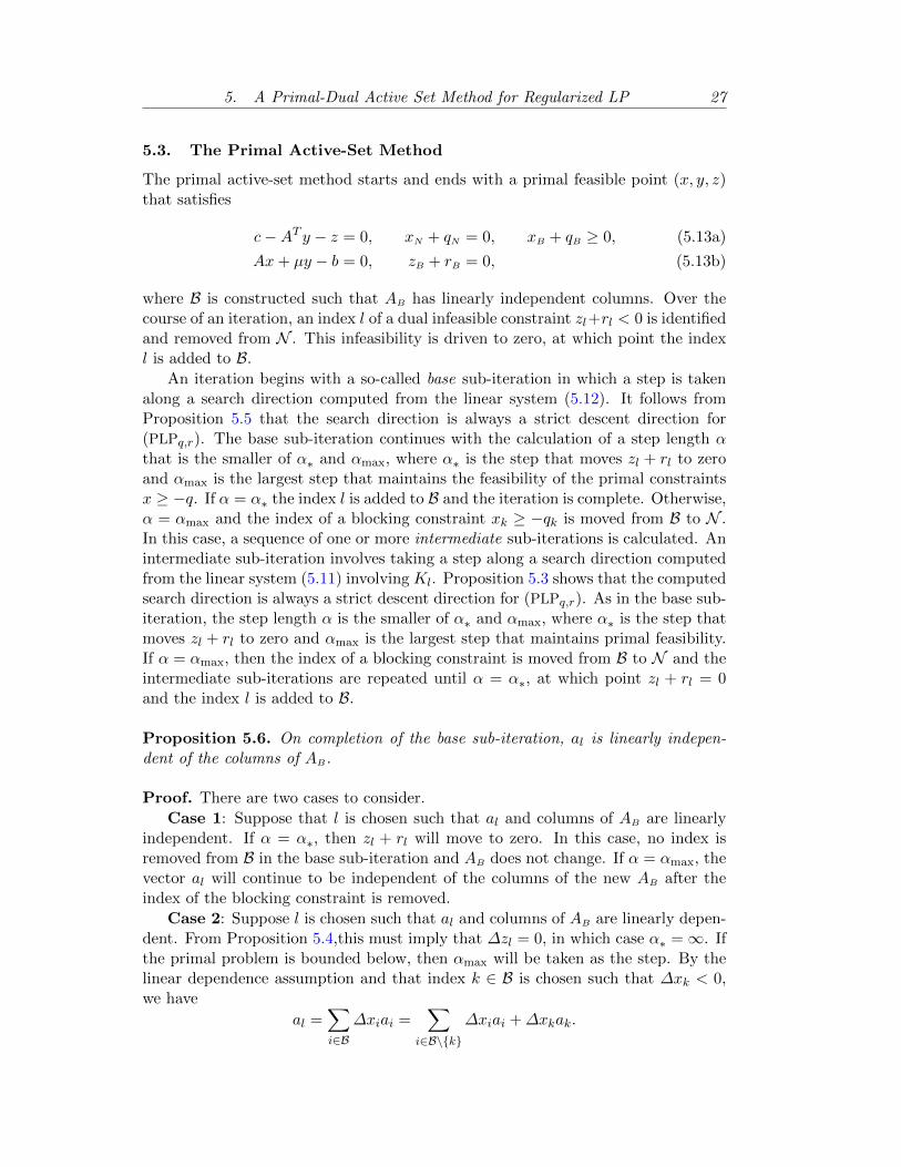
5.3. The Primal Active-Set Method
The primal active-set method starts and ends with a primal feasible point (x, y, z)that satisfies
c�AT y � z = 0, xN + qN = 0, xB + qB � 0, (5.13a)
Ax+ µy � b = 0, zB + rB = 0, (5.13b)
where B is constructed such that AB has linearly independent columns. Over thecourse of an iteration, an index l of a dual infeasible constraint z
l
+rl
< 0 is identifiedand removed from N . This infeasibility is driven to zero, at which point the indexl is added to B.
An iteration begins with a so-called base sub-iteration in which a step is takenalong a search direction computed from the linear system (5.12). It follows fromProposition 5.5 that the search direction is always a strict descent direction for(PLP
q,r
). The base sub-iteration continues with the calculation of a step length ↵that is the smaller of ↵⇤ and ↵
max
, where ↵⇤ is the step that moves zl
+ rl
to zeroand ↵
max
is the largest step that maintains the feasibility of the primal constraintsx � �q. If ↵ = ↵⇤ the index l is added to B and the iteration is complete. Otherwise,↵ = ↵
max
and the index of a blocking constraint xk
� �qk
is moved from B to N .In this case, a sequence of one or more intermediate sub-iterations is calculated. Anintermediate sub-iteration involves taking a step along a search direction computedfrom the linear system (5.11) involving K
l
. Proposition 5.3 shows that the computedsearch direction is always a strict descent direction for (PLP
q,r
). As in the base sub-iteration, the step length ↵ is the smaller of ↵⇤ and ↵
max
, where ↵⇤ is the step thatmoves z
l
+ rl
to zero and ↵max
is the largest step that maintains primal feasibility.If ↵ = ↵
max
, then the index of a blocking constraint is moved from B to N and theintermediate sub-iterations are repeated until ↵ = ↵⇤, at which point z
l
+ rl
= 0and the index l is added to B.
Proposition 5.6. On completion of the base sub-iteration, al
is linearly indepen-dent of the columns of AB.
Proof. There are two cases to consider.Case 1: Suppose that l is chosen such that a
l
and columns of AB are linearlyindependent. If ↵ = ↵⇤, then z
l
+ rl
will move to zero. In this case, no index isremoved from B in the base sub-iteration and AB does not change. If ↵ = ↵
max
, thevector a
l
will continue to be independent of the columns of the new AB after theindex of the blocking constraint is removed.
Case 2: Suppose l is chosen such that al
and columns of AB are linearly depen-dent. From Proposition 5.4,this must imply that �z
l
= 0, in which case ↵⇤ =1. Ifthe primal problem is bounded below, then ↵
max
will be taken as the step. By thelinear dependence assumption and that index k 2 B is chosen such that �x
k
< 0,we have
al
=X
i2B�x
i
ai
=X
i2B\{k}
�xi
ai
+�xk
ak
.

28 Anti-Cycling Methods for Linear Programming
After removing the index k from B, the column al
cannot be written as a linearcombination of columns of the new AB, which implies that they must be linearlyindependent.
Proposition 5.7. The matrix Kl
will remain nonsingular during a sequence of in-termediate sub-iterations.
Proof. Follows from Proposition 5.2 and Proposition 5.6.
It is important to note that if ↵ = ↵max
in the base sub-iteration, then at leastone intermediate sub-iteration is needed because the dual infeasibility could not beeliminated by taking the longer step ↵ = ↵⇤. It is also possible for ↵ to be zeroin a base or intermediate sub-iteration. However, once a zero step is taken, anindex will be deleted from B, and the execution of an intermediate sub-iterationmust follow. The intermediate sub-iterations continue until a nonzero step is takenand z
l
+ rl
becomes non-negative. The degenerate case is considered in Section 5.5below, where it is shown that in the worst case, if all the indices are deleted fromB by the intermediate sub-iterations, then the search direction must be nonzero byProposition 5.10 and ↵ > 0 will drive z
l
+ rl
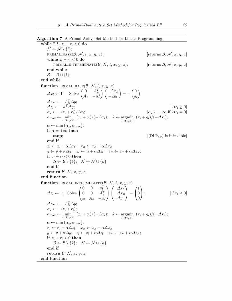
to zero.The primal active-set method is described in Algorithm 7.
5. A Primal-Dual Active Set Method for Regularized LP 29
Algorithm 7 A Primal Active-Set Method for Linear Programming.while 9 l : z
l
+ rl
< 0 doN N \ {l};primal base(B, N , l, x, y, z); [returns B, N , x, y, z]while z
l
+ rl
< 0 doprimal intermediate(B, N , l, x, y, z); [returns B, N , x, y, z]
end whileB B [ {l};
end while
function primal base(B, N , l, x, y, z)
�xl
1; Solve
✓
0 AT
B
AB �µI
◆✓
�xB
��y
◆
= �✓
0al
◆
;
�zN �AT
N�y;�z
l
�aTl
�y; [�zl
� 0]↵⇤ �(zl + r
l
)/�zl
; [↵⇤ +1 if �zl
= 0]↵max
mini:�xi<0
(xi
+ qi
)/(��xi
); k argmini:�xi<0
(xi
+ qi
)/(��xi
);
↵ min�
↵⇤,↵max
�
;if ↵ = +1 then
stop; [(DLPq,r
) is infeasible]end ifxl
xl
+ ↵�xl
; xB xB + ↵�xB;y y + ↵�y; z
l
zl
+ ↵�zl
; zN zN + ↵�zN ;if z
l
+ rl
< 0 thenB B \ {k}; N N [ {k};
end ifreturn B, N , x, y, z;
end function
function primal intermediate(B, N , l, x, y, z)
�zl
1; Solve
0
@
0 0 aTl
0 0 AT
B
al
AB �µI
1
A
0
@
�xl
�xB
��y
1
A =
0
@
100
1
A; [�xl
� 0]
�zN �AT
N�y;↵⇤ �(zl + r
l
);↵max
mini:�xi<0
(xi
+ qi
)/(��xi
); k argmini:�xi<0
(xi
+ qi
)/(��xi
);
↵ min�
↵⇤,↵max
�
;xl
xl
+ ↵�xl
; xB xB + ↵�xB;y y + ↵�y; z
l
zl
+ ↵�zl
; zN zN + ↵�zN ;if z
l
+ rl
< 0 thenB B \ {k}; N N [ {k};
end ifreturn B, N , x, y, z;
end function

30 Anti-Cycling Methods for Linear Programming
5.4. The Dual Active-Set Method
The dual active-set method starts and ends with a dual feasible point (x, y, z) thatsatisfies the equations
c�ATy � z = 0, xN + qN = 0, (5.14a)
Ax+ µy � b = 0, zB + rB = 0, zN + rN � 0, (5.14b)
where B is constructed so that AB has linearly independent columns. At eachiteration, an index l of a primal-infeasible constraint x
l
+ ql
< 0 is identified andremoved from B. This infeasibility is driven to zero over the course of an iteration,at which point the index l is added to N .
An iteration begins with a so-called base sub-iteration in which a step is takenalong a direction computed from the linear system (5.11). It follows from Propo-sition 5.3 that the search direction is always a strict ascent direction for (DLP
q,r
).The base sub-iteration continues with the calculation of a step length ↵ that is thesmaller of ↵⇤ and ↵
max
, where ↵⇤ is the step that moves xl
+ ql
to zero, and ↵max
is the largest step that maintains the feasibility of the dual constraints z � �r.If ↵ = ↵⇤ the index l is added to B and the iteration is complete. Otherwise,↵ = ↵
max
, and the index of a blocking constraint zk
� �rk
is moved from N to B.In this case a sequence of one or more intermediate sub-iterations is calculated. Anintermediate sub-iteration involves taking a step along the primal-dual search direc-tion (�xB,�y) satisfying the equations (5.12). This direction satisfies the equations(5.11) with �x
l
= 1 and �zl
= 0. It follows from Proposition 5.5 that the searchdirection is a strict ascent direction for (DLP
q,r
). As in the base sub-iteration, thestep ↵ is the smaller of ↵⇤ and ↵
max
, where ↵⇤ is the step that moves zl
+ rl
to zero,and ↵
max
is the largest step that maintains dual feasibility. If ↵ = ↵max
the indexof a blocking constraint is moved from N to B and the intermediate sub-iterationsare repeated until ↵ = ↵⇤, in which case x
l
+ ql
= 0 and the index l is added to N .If B is empty at the beginning of the dual algorithm, then only the base sub-
iteration is needed to drive xl
+ql
to zero. Otherwise, if B is nonempty and ↵ = ↵max
in the base sub-iteration then at least one intermediate sub-iteration is needed.
Proposition 5.8. The matrix AB always has linearly independent columns at theend of the dual algorithm.
Proof. If al
and the columns of AB are linearly dependent at the beginning of anintermediate sub-iteration, then Proposition 5.4 gives �z = 0. In this case, the set{i : �z
i
< 0} is empty and ↵ must take the value ↵⇤, then the updated primalviolation x
l
+ ql
is zero. At this point no more indices will be added to B, the indexl is added to N , and the full-rank matrix is not changed.
The dual active-set method is given in Algorithm 8.
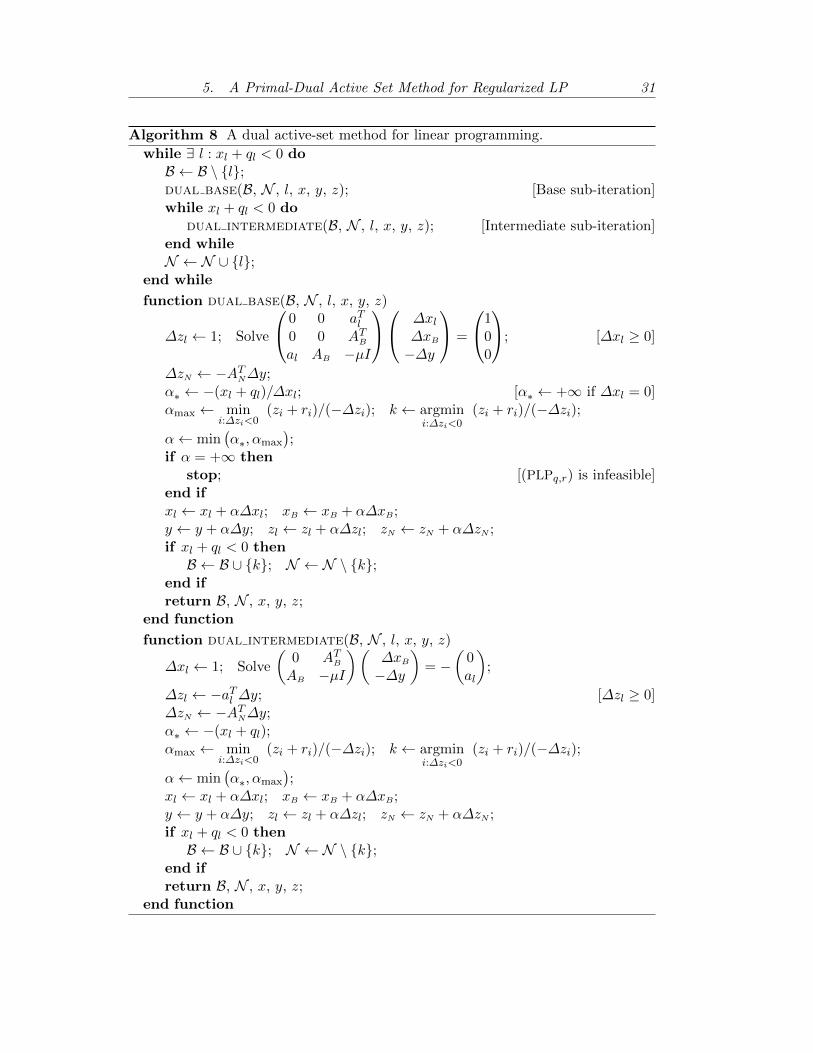
5. A Primal-Dual Active Set Method for Regularized LP 31
Algorithm 8 A dual active-set method for linear programming.while 9 l : x
l
+ ql
< 0 doB B \ {l};dual base(B, N , l, x, y, z); [Base sub-iteration]while x
l
+ ql
< 0 dodual intermediate(B, N , l, x, y, z); [Intermediate sub-iteration]
end whileN N [ {l};
end while
function dual base(B, N , l, x, y, z)
�zl
1; Solve
0
@
0 0 aTl
0 0 AT
B
al
AB �µI
1
A
0
@
�xl
�xB
��y
1
A =
0
@
100
1
A; [�xl
� 0]
�zN �AT
N�y;↵⇤ �(xl + q
l
)/�xl
; [↵⇤ +1 if �xl
= 0]↵max
mini:�zi<0
(zi
+ ri
)/(��zi
); k argmini:�zi<0
(zi
+ ri
)/(��zi
);
↵ min�
↵⇤,↵max
�
;if ↵ = +1 then
stop; [(PLPq,r
) is infeasible]end ifxl
xl
+ ↵�xl
; xB xB + ↵�xB;y y + ↵�y; z
l
zl
+ ↵�zl
; zN zN + ↵�zN ;if x
l
+ ql
< 0 thenB B [ {k}; N N \ {k};
end ifreturn B, N , x, y, z;
end function
function dual intermediate(B, N , l, x, y, z)
�xl
1; Solve
✓
0 AT
B
AB �µI
◆✓
�xB
��y
◆
= �✓
0al
◆
;
�zl
�aTl
�y; [�zl
� 0]�zN �AT
N�y;↵⇤ �(xl + q
l
);↵max
mini:�zi<0
(zi
+ ri
)/(��zi
); k argmini:�zi<0
(zi
+ ri
)/(��zi
);
↵ min�
↵⇤,↵max
�
;xl
xl
+ ↵�xl
; xB xB + ↵�xB;y y + ↵�y; z
l
zl
+ ↵�zl
; zN zN + ↵�zN ;if x
l
+ ql
< 0 thenB B [ {k}; N N \ {k};
end ifreturn B, N , x, y, z;
end function

32 Anti-Cycling Methods for Linear Programming
5.5. Degeneracy
An iteration is said to be degenerate if a zero step is defined in each of the baseand intermediate sub-iterations. Specifically, the primal problem is nondegenerateif a nonzero step is taken at every base sub-iteration. The nonsingularity of theregularized term µI will guarantee that the primal problem is nondegenerate.
We require that the constrained gradient AB to be linearly independent frombeginning, and our method for adding and deleting constraints from working set forsubsequent working set will still maintain the property of linearly independence.
Proposition 5.9. If �zl
> 0, Kl
nonsingular and µ 6= 0, then the primal step isnondegenerate.
Proof. The proof follows from the fact that �xl
= µ/aTl
Pal
> 0, where P =(I �AB(AT
BAB)�1AT
B).
Proposition 5.10. The primal-dual active-set method does not cycle.
Proof. Suppose that at the end of the intermediate sub-iterations, every variablein B is deleted. The equation becomes
✓
0 aTl
al
�µI
◆✓
�xl
��y
◆
=
✓
10
◆
. (5.15)
�
�xl
��y�
T
has the unique solution
✓
�xl
��y
◆
=1
kal
k2
✓
µal
◆
as µ > 0, al
> 0.
5.6. Combining Primal and Dual Active-set Methods
The primal active-set method proposed in Section 5.3 may be used to solve (PLPq,r
)for a given initial basis B satisfying the conditions (5.13). An appropriate initialpoint may be found by solving a conventional phase-1 linear program. Alternatively,the dual active-set method of Section 5.4 may be used in conjunction with an ap-propriate phase 1 procedure to solve the quadratic program (PLP
q,r
) for a giveninitial basis B satisfying the conditions (5.14). An alternative to the conventionalphase-1/phase-2 approach is to create a pair of coupled quadratic programs fromthe original by simultaneously shifting the bound constraints. The idea is to solve ashifted dual problem to define an initial feasible point for the primal, or vice-versa.This strategy provides an alternative to the conventional phase-1/phase-2 approachthat utilizes the phase-1 objective function while finding a feasible point.
An algorithm that combines the primal and dual active-set methods is given inAlgorithm 9. The algorithm begins with a second-order consistent basis satisfying

5. A Primal-Dual Active Set Method for Regularized LP 33
(5.5) and (5.6). If the initial point is both primal and dual feasible then the triple (x,y, z) is an optimal solution and the algorithm is terminated. If x is primal feasible,then the primal active-set method PRIMAL LP of Algorithm 7 is used to find anoptimal solution. If z is dual feasible, then the dual active-set method DUAL LP ofAlgorithm 8 is used to find an optimal solution. If the initial point is neither primalnor dual feasible, then one of the shifts q or r can be defined to make the initialpoint either primal or dual feasible.
5.6.1. Shifting the primal problem
Assume that the given initial point is neither primal nor dual feasible. If we chooseto shift the primal problem, the shifts are defined as follows.
1. Define the shifts r and q such that r = 0 and qN = 0, qB = max{�xB, 0}.
2. Compute the solution of (PLPq,r
).
3. Compute a point (x(1), y(1), z(1)) satisfying (5.5) and (5.6).
4. Starting at the point (x(1), y(1), z(1)), solve (DLP0,0
).
After applying the shifts in Step 1, the point x satisfies x + q � 0, i.e., x is aninitial primal-feasible point for (PLP
q,r
). The optimal solution of the primal problem(PLP
q,r
) solved in Step 2 satisfies
c�ATy(1) � z(1) = 0, x(1)N + qN = 0, x(1)B + qB � 0,
Ax(1) + µy(1) � b = 0, z(1)B = 0, z(1)N � 0.
Without the shift, this solution may violate (5.5) and (5.6), in which case x(1) mustbe recomputed in Step 3 by solving the linear least-squares problem
minimizex2Rt
kABx� b+ µy(1)k.
The point (x(1), y(1), z(1)) found in Step 3 will be dual feasible for the originalproblem and Step 4 will compute the required optimal solution.
5.6.2. Shifting the dual problem
Again, assume that the given initial point is neither primal nor dual feasible. If wechoose to shift the dual problem, the shifts are defined as follows:
1. Define the shifts q and r such that q = 0, rB = 0 and rN = max{�zN , 0}.
2. Compute a solution of (DLPq,r
).
3. Compute a point (x(1), y(1), z(1)) satisfying (5.5) and (5.6).
4. Starting at the point (x(1), y(1), z(1)), solve (PLP0,0
).

34 Anti-Cycling Methods for Linear Programming
After applying the shifting procedure of Step 1, the point z satisfies z + r � 0, i.e.,z is an initial dual feasible point for (DLP
q,r
). The optimal solution of (DLPq,r
)satisfies
c�ATy(1) � z(1) = 0, x(1)N = 0, x(1)B � 0,
Ax(1) + µy(1) � b = 0, z(1)B + rB = 0, z(1)N + rN � 0.
Without the shift, this solution may violate (5.5) and (5.6), in which case y(1) andz(1) must be recomputed in Step 3 using
y(1) =1
µ(b�ABx
(1)
B ) and z(1)N = cN �AT
Ny(1).
The point (x(1), y(1), z(1)) computed in Step 3 will be primal feasible, and Step 4will compute an optimal solution for the original problem.

6. Matrix Factorizations and Updating 35
Algorithm 9 Primal-Dual Active Set Method for Regularized LPinput: A, b, c, µ, choice;Find a second-order consistent basis B;
Solve
✓
0 AT
B
AB �µI
◆✓
xB
�y
◆
=
✓
�cBb
◆
;
q = 0; r = 0; [Initialize the shifts]xN = 0; zB = 0; zN = cN �AT
Ny;if x � 0 and z � 0 then
stop; [(x, y, z) is optimal]else if x � 0 then [Primal feasible]
primal lp(B, N , x, y, z, A, b, c, q, r, µ);else if z � 0 then [Dual feasible]
dual lp(B, N , x, y, z, A, b, c, q, r, µ);else [Neither primal nor dual feasible]
if choice = primal first thenqN = 0; qB = max{�xB, 0}; [Redefine the shift q][B, N ]=primal lp(B, N , A, b, c, q, r, µ);
Solve
✓
0 AT
B
AB �µI
◆✓
xB
�y
◆
=
✓
�cBb
◆
;
xN = 0; zB = 0; zN = cN �AT
Ny; q = 0;dual lp(B, N , x, y, z, A, b, c, q, r, µ);
else if choice = dual first thenrB = 0; rN = max{�zN , 0}; [Redefine the shift r][B, N ]=dual lp(B, N , A, b, c, q, r, µ);
Solve
✓
0 AT
B
AB �µI
◆✓
xB
�y
◆
=
✓
�cBb
◆
;
xN = 0; zB = 0; zN = cN �AT
Ny; r = 0;primal lp(B, N , x, y, z, A, b, c, q, r, µ);
end ifend ifreturn x, y, z, B, N ;
6. Matrix Factorizations and Updating
When solving the linear least-squares problem minx2Rm kAx� bk it is crucial that
a factorization of the matrix A is used instead of directly computing the inverse ofATA for the normal equations. Consider an m⇥ n matrix A with m > n. The QRfactorization of A is given by
QTA =
✓
R0
◆
, (6.1)
where Q is an orthogonal matrix of dimension m⇥m, and R is an upper-triangularmatrix of dimension n⇥ n.
It is also necessary to update this factorization when columns or the rows of Aare added, deleted, or both.
36 Anti-Cycling Methods for Linear Programming
6.1. Using the QR Decomposition for Solving Least-Squares Problems
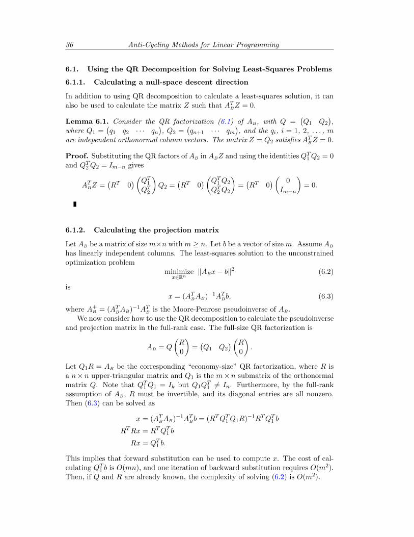
6.1.1. Calculating a null-space descent direction
In addition to using QR decomposition to calculate a least-squares solution, it canalso be used to calculate the matrix Z such that AT
BZ = 0.
Lemma 6.1. Consider the QR factorization (6.1) of AB, with Q =�
Q1
Q2
�
,where Q
1
=�
q1
q2
· · · qn
�
, Q2
=�
qn+1
· · · qm
�
, and the qi
, i = 1, 2, . . . , mare independent orthonormal column vectors. The matrix Z = Q
2
satisfies AT
BZ = 0.
Proof. Substituting the QR factors of AB in ABZ and using the identitiesQT
1
Q2
= 0and QT
2
Q2
= Im�n
gives
AT
BZ =�
RT 0�
✓
QT
1
QT
2
◆
Q2
=�
RT 0�
✓
QT
1
Q2
QT
2
Q2
◆
=�
RT 0�
✓
0Im�n
◆
= 0.
6.1.2. Calculating the projection matrix
Let AB be a matrix of sizem⇥n withm � n. Let b be a vector of sizem. Assume AB
has linearly independent columns. The least-squares solution to the unconstrainedoptimization problem
minimizex2Rn
kABx� bk2 (6.2)
isx = (AT
BAB)�1AT
Bb, (6.3)
where A+
B = (AT
BAB)�1AT
B is the Moore-Penrose pseudoinverse of AB.We now consider how to use the QR decomposition to calculate the pseudoinverse
and projection matrix in the full-rank case. The full-size QR factorization is
AB = Q
✓
R0
◆
=�
Q1
Q2
�
✓
R0
◆
.
Let Q1
R = AB be the corresponding “economy-size” QR factorization, where R isa n⇥ n upper-triangular matrix and Q
1
is the m⇥ n submatrix of the orthonormalmatrix Q. Note that QT
1
Q1
= Ik
but Q1
QT
1
6= In
. Furthermore, by the full-rankassumption of AB, R must be invertible, and its diagonal entries are all nonzero.Then (6.3) can be solved as
x = (AT
BAB)�1AT
Bb = (RTQT
1
Q1
R)�1RTQT
1
b
RTRx = RTQT
1
b
Rx = QT
1
b.
This implies that forward substitution can be used to compute x. The cost of cal-culating QT
1
b is O(mn), and one iteration of backward substitution requires O(m2).Then, if Q and R are already known, the complexity of solving (6.2) is O(m2).

6. Matrix Factorizations and Updating 37
Now consider the calculation of the orthogonal projection matrix onto range(AB),
P = AB(AT
BAB)�1AT
B = Q1
R(RTR)�1RTQT
1
= Q1
RR�1R�TRTQT
1
= Q1
In
QT
1
= Q1
QT
1
.
Similarly, the orthogonal projection onto null(AT
B) can be calculated as
M = In
�Q1
QT
1
, (6.4)
orM = Z(ZTZ)�1ZT , (6.5)
where the columns of Z form a basis for null(AT
B). By using the result from (6.1)
Z(ZTZ)�1ZT = Q2
(QT
2
Q2
)�1QT
2
= Q2
Im�n
QT
2
= Q2
QT
2
.
When m� n it is more e�cient to store only Q1
and calculate the steepest-descentdirection in the null space, i.e., p = �Z(ZTZ)�1ZT c using (6.4),
p = (Q1
QT
1
� I)c.
The cost of calculating the steepest-descent direction in null(AT
B) is approximately2mn+m flops.
6.1.3. Solving the KKT equations
By using the results above, the solution of the linear system (5.11) can be writtenas
�xl
= �µ,
�xB = ��R�1QT
1
al
,
��y = �(al
+AB�xB) = �(al
�Q1
QT
1
al
),
where� = aT
l
Mal
= aTl
(In
�Q1
QT
1
)al
.
The cost of computing (5.11) by given QR decomposition is O(m2).
6.2. Updating the QR Factorization
It is critical to consider the modification as recomputing the QR factorization is tooexpensive as it requires approximately mn2 floating-point operations.
Three kinds of modification of the matrix Ak
are considered:
1. a rank-one change of Ak
;
2. the deletion and addition of a column of Ak
; and

38 Anti-Cycling Methods for Linear Programming
3. the deletion and addition of a row of Ak
.
First, consider two basic transformations that are essential tools for matrix updating—Givens rotations and Householder transformations.
Lemma 6.2. (Givens Rotation) Given x =
✓
x1
x2
◆
, with at least one of the quan-
tities x1
and x2
nonzero, then there exists an orthogonal matrix
G =
✓
c s�s c
◆
with c2 + s2 = 1 such that
Gx =
✓
(x21
+ x22
)1/2
0
◆
.
Proof. The result follows directly with c and s defined as
c =x1
(x21
+ x2
)1/2and s =
x2
(x21
+ x2
)1/2. (6.6)
To exploit the symmetric structure, we instead define the symmetric Givensmatrix
G =
✓
c ss �c
◆
with the same c and s as in (6.6).
Lemma 6.3. (Householder transformation) Given a non-zero vector v 2 Rm,there exists an orthogonal matrix Q such that
Qv = ��kvk e1
with e1
= (1, 0, . . . , 0)T and � = sign(v1
).
Proof. Define
Q = Im
� 2uuT
uTu, with u = v + �||v||e
1
.
6.3. Modification after a Rank-one Change
Given the QR decomposition of the matrix Ak
2 Rm⇥n
Ak
= Qk
✓
Rk
0
◆
,
6. Matrix Factorizations and Updating 39
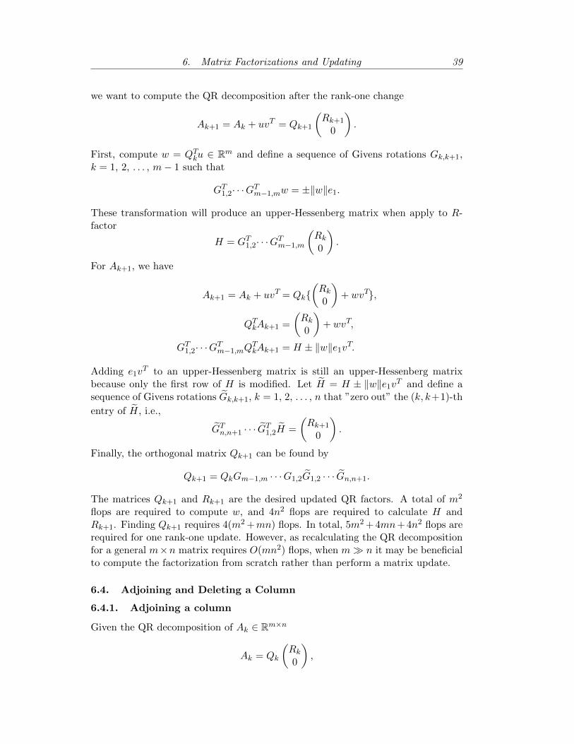
we want to compute the QR decomposition after the rank-one change
Ak+1
= Ak
+ uvT = Qk+1
✓
Rk+1
0
◆
.
First, compute w = QT
k
u 2 Rm and define a sequence of Givens rotations Gk,k+1
,k = 1, 2, . . . , m� 1 such that
GT
1,2
· · ·GT
m�1,m
w = ±kwke1
.
These transformation will produce an upper-Hessenberg matrix when apply to R-factor
H = GT
1,2
· · ·GT
m�1,m
✓
Rk
0
◆
.
For Ak+1
, we have
Ak+1
= Ak
+ uvT = Qk
{✓
Rk
0
◆
+ wvT},
QT
k
Ak+1
=
✓
Rk
0
◆
+ wvT,
GT
1,2
· · ·GT
m�1,m
QT
k
Ak+1
= H ± kwke1
vT.
Adding e1
vT to an upper-Hessenberg matrix is still an upper-Hessenberg matrixbecause only the first row of H is modified. Let eH = H ± kwke
1
vT and define asequence of Givens rotations eG
k,k+1
, k = 1, 2, . . . , n that ”zero out” the (k, k+1)-th
entry of eH, i.e.,
eGT
n,n+1
· · · eGT
1,2
eH =
✓
Rk+1
0
◆
.
Finally, the orthogonal matrix Qk+1
can be found by
Qk+1
= Qk
Gm�1,m
· · ·G1,2
eG1,2
· · · eGn,n+1
.
The matrices Qk+1
and Rk+1
are the desired updated QR factors. A total of m2
flops are required to compute w, and 4n2 flops are required to calculate H andR
k+1
. Finding Qk+1
requires 4(m2+mn) flops. In total, 5m2+4mn+4n2 flops arerequired for one rank-one update. However, as recalculating the QR decompositionfor a general m⇥n matrix requires O(mn2) flops, when m� n it may be beneficialto compute the factorization from scratch rather than perform a matrix update.
6.4. Adjoining and Deleting a Column
6.4.1. Adjoining a column
Given the QR decomposition of Ak
2 Rm⇥n
Ak
= Qk
✓
Rk
0
◆
,

40 Anti-Cycling Methods for Linear Programming
we require the QR decomposition after appending one column vector ak+1
, i.e.,
Ak+1
=�
Ak
ak+1
�
First, let bk+1
= QT
k
ak+1
. Premultiply Ak+1
by Qk
and partition the matrix
QT
k
Ak+1
=
✓
Rk
0bk+1
◆
=
✓
Rk
sk
0 v
◆
with bk+1
=
✓
sk
v
◆
, (6.7)
where sk
is a vector of dimension n and v is a vector of dimension m� n. Using aHouseholder transformation of the form (6.3) we define
u = v + �||v||e1
, (6.8)
bH = Im�k
� 2uuT
uTu, (6.9)
with e1
the (m� n)-vector e1
= (1, 0, . . . , 0)T . Let
H =
✓
Im
0
0 bH
◆
.
As H is symmetric, the equation (6.7) can be premultiplied by HT to give
HTQT
k
Ak+1
=
✓
Im
0
0 bH
◆✓
Rk
sk
0 v
◆
=
0
@
Rk
sk
0 ��||v||e1
0 0
1
A ,
QT
k+1
Ak+1
=
✓
Rk+1
0
◆
,
with � = sign(v1
), and Qk+1
= Qk
H.
6.4.2. Removing a column
Given the QR decomposition of Ak
2 Rm⇥n
Ak
= Qk
✓
Rk
0
◆
,
we require the QR factorization when the j-th column is removed from Ak
, where1 j n. An explicit method proposed by Golub and Saunders [14] defines
Ak+1
=�
a1
· · · aj�1
aj+1
· · · an
�
,
where ai
is the i-th column of Ak
. Premultiplying by QT
k
gives
QT
k
Ak+1
=�
r1
· · · rj�1
rj+1
· · · rn
�
,
with ri
is the i-th column vector of Rk
. We then define a sequence of Givenstransformations G
i,i+1
, i = j, . . . , n� 1, where Gi,i+1
zeros out the i-th element ofthe (i+ 1)-th row. The orthogonal matrix Q
k+1
is found by
Qk+1
= Qk
GT
j,j+1
· · ·GT
n�1,n
.

6. Matrix Factorizations and Updating 41
The matrix Rk+1
is found by explicitly calculating the last (n � j + 1)-th columnsas
QT
k+1
Ak+1
=
✓
Rk+1
0
◆
,
where the first (j � 1) columns of Rk+1
are the same as those of Rk
.
6.5. Adjoining and Deleting a Row
6.5.1. Adjoining a row
Given a QR decomposition of Ak
2 Rm⇥n
Ak
= Qk
✓
Rk
0
◆
,
we require the QR decomposition after adjoining the row vector ak+1
2 Rn, i.e.,
Ak+1
=
✓
Ak
aTk+1
◆
= Qk+1
✓
Rk+1
0
◆
.
First, we apply an orthogonal matrix diag(Qk
, 1),
✓
Qk
00 1
◆✓
Ak
aTk+1
◆
=
0
@
Rk
0aTk+1
1
A = ⇧n+1,m+1
0
@
Rk
aTk+1
0
1
A ,
where ⇧n+1,m+1
is a permutation matrix that interchanges rows n+ 1 and m+ 1.Then use a sequence of Givens rotations G
i,n+1
, i = 1, . . . , n where Gi,n+1
eliminates the i-th element of the (n+ 1)-th row,
Gn,n+1
Gn�1,n+1
· · ·G1,n+1
⇧n+1,m+1
✓
Rk
aTk+1
◆
=
✓
Rk+1
0
◆
,
and the updated Qk+1
becomes
Qk+1
=
✓
Qk
00 1
◆
⇧n+1,m+1
GT
1,n+1
· · ·GT
n,n+1
.
The updating procedure is stable and requires approximately 2n2 operations withstandard Givens rotations.
6.5.2. Deleting a row
Given a QR decomposition of the matrix Ak
2 Rm⇥n
Ak
=
✓
aT1
Ak+1
◆
= Qk
✓
Rk
0
◆
,

42 Anti-Cycling Methods for Linear Programming
without loss of generality, we want to compute the QR decomposition of Ak+1
, i.e.,the submatrix of A
k+1
without the first row,
Ak+1
= Qk+1
✓
Rk+1
0
◆
.
Note that the removal of k-th row can be done by the same procedure except thatwe premultiply a permutation matrix ⇧
1,k
to Ak
and Qk
in order to interchangerow 1 and row k. The algorithm given below is then applied to ⇧
1,k
Ak
and ⇧1,k
Qk
instead.First find the QR decomposition of
�
e1
Ak
�
,
QT
k
�
e1
Ak
�
=
✓
q1
Rk
0
◆
.
where q1
is the first row of Qk
.Then define a sequence of Givens transformation G
i,i+1
, i = 1, . . . , m� 1 suchthat
GT
1,2
· · ·GT
m�1,m
q1
= ↵e1
, k↵k = 1.
Then we have
GT
1,2
· · ·GT
m�1,m
✓
q1
Rk
0
◆
=
0
@
↵ vT
0 Rk+1
0 0
1
A .
In addition, we compute Qk+1
as below,
Qk
Gm�1,m
· · ·G1,2
=
✓
↵ 00 Q
k+1
◆
.
Hence, we have
Ak
=
✓
aT1
Ak+1
◆
= Qk
✓
Rk
0
◆
= Qk
Gm�1,m
· · · , G1,2
GT
1,2
· · ·GT
m�1,m
✓
Rk
0
◆
=
✓
↵ 00 Q
k+1
◆
0
@
vT
Rk+1
0
1
A .
This algorithm for removing a row can be regarded as a special case of updatingafter a rank-one change with u = �e
1
and v = a1
.
6.6. Other Factorization Methods
6.6.1. The symmetric indefinite factorization
When a matrix K 2 Rn⇥n is symmetric positive definite, the Cholesky factorizationK = LLT can be used to solve the linear system Kx = f . The Cholesky algorithm
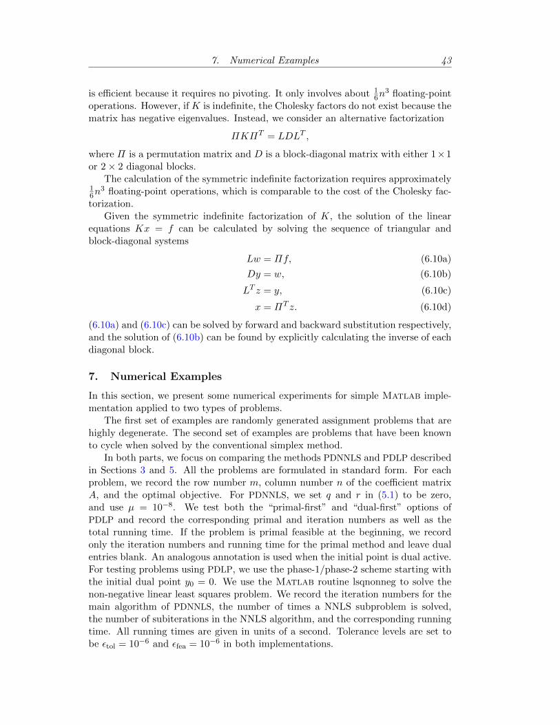
7. Numerical Examples 43
is e�cient because it requires no pivoting. It only involves about 1
6
n3 floating-pointoperations. However, if K is indefinite, the Cholesky factors do not exist because thematrix has negative eigenvalues. Instead, we consider an alternative factorization
⇧K⇧T = LDLT ,
where ⇧ is a permutation matrix and D is a block-diagonal matrix with either 1⇥1or 2⇥ 2 diagonal blocks.
The calculation of the symmetric indefinite factorization requires approximately1
6
n3 floating-point operations, which is comparable to the cost of the Cholesky fac-torization.
Given the symmetric indefinite factorization of K, the solution of the linearequations Kx = f can be calculated by solving the sequence of triangular andblock-diagonal systems
Lw = ⇧f, (6.10a)
Dy = w, (6.10b)
LT z = y, (6.10c)
x = ⇧T z. (6.10d)
(6.10a) and (6.10c) can be solved by forward and backward substitution respectively,and the solution of (6.10b) can be found by explicitly calculating the inverse of eachdiagonal block.
7. Numerical Examples
In this section, we present some numerical experiments for simple Matlab imple-mentation applied to two types of problems.
The first set of examples are randomly generated assignment problems that arehighly degenerate. The second set of examples are problems that have been knownto cycle when solved by the conventional simplex method.
In both parts, we focus on comparing the methods PDNNLS and PDLP describedin Sections 3 and 5. All the problems are formulated in standard form. For eachproblem, we record the row number m, column number n of the coe�cient matrixA, and the optimal objective. For PDNNLS, we set q and r in (5.1) to be zero,and use µ = 10�8. We test both the “primal-first” and “dual-first” options ofPDLP and record the corresponding primal and iteration numbers as well as thetotal running time. If the problem is primal feasible at the beginning, we recordonly the iteration numbers and running time for the primal method and leave dualentries blank. An analogous annotation is used when the initial point is dual active.For testing problems using PDLP, we use the phase-1/phase-2 scheme starting withthe initial dual point y
0
= 0. We use the Matlab routine lsqnonneg to solve thenon-negative linear least squares problem. We record the iteration numbers for themain algorithm of PDNNLS, the number of times a NNLS subproblem is solved,the number of subiterations in the NNLS algorithm, and the corresponding runningtime. All running times are given in units of a second. Tolerance levels are set tobe ✏
tol
= 10�6 and ✏fea
= 10�6 in both implementations.

44 Anti-Cycling Methods for Linear Programming
7.1. Highly Degenerate Problems
7.1.1. Test problems
Below we give the pseudocode for the assignment problem. The pseudocode returnsthe matrix A, and vectors b and c associated with a linear program in standard form
minimizex2Rn
cTx subject to Ax = b, x � 0.
Given an integer n, the assignment algorithm returns A 2 R(2n�1)⇥n
2, b 2 R2n�1
and c 2 Rn
2, where A is sparse with unit entries. The matrix A has significantly
more columns than rows, which increases the chance of selecting a dependent basisin a conventional active-set method. The problem is highly degenerate.
Algorithm 10 The assignment problem.
function assign(n)C = rand(n);for i = 1 to n do
b(i, 1) = 1;b(n+ i, 1) = 1;for j = 1 to n do
c(n(i� 1) + j, 1) = C(i, j);A(i, n(i� 1) + j) = 1;A(n+ i, n(j � 1) + i) = 1;
end forend forreturn A, b, c;
end function
7.1.2. Computational results
In this section we present the results of numerical experiments on the assignmentproblems for n = 25, 50, 75, 100, 125, 150, 200, and 300. As the cost vector c isnon-negative, the initial point y
0
= 0 is dual feasible for PDNNLS and it is necessaryto solve only the phase 1 problem for this method. For this reason, in all the tablesfor PDNNLS, only the iteration numbers and running times for the phase 1 problemare recorded.

7. Numerical Examples 45
Table 1: Results for PDNNLS on Assignment Problems
PHASE 1m n Objective Itn NNLS-Itn NNLS-Sub Time
49 625 1.2766622E+00 37 622 1 0.035299 2500 1.6111842E+00 113 5376 268 0.3951
149 5625 1.5963300E+00 185 14461 362 1.2308199 10000 1.7456917E+00 225 20723 610 1.9004249 15625 1.6131899E+00 257 28257 737 2.9211299 25000 1.5795925E+00 303 38904 909 4.4300399 40000 1.6880131E+00 504 109440 3938 17.5161599 90000 1.5619877E+00 693 212082 7497 45.3444
Table 2: Results for PDLP on Assignment Problems
Primal-First Dual-Firstm n Objective Itn P-Itn D-Itn Time Itn P-Itn D-Itn Time
49 625 1.2766622E+00 64 46 18 0.0322 140 92 48 0.041599 2500 1.6111842E+00 122 22 100 0.1468 358 250 108 0.2174
149 5625 1.5963300E+00 226 62 164 0.4080 699 377 322 0.7280199 10000 1.7456917E+00 444 133 311 1.0075 1083 641 442 1.6531249 15625 1.6131899E+00 374 59 315 1.5745 1200 810 390 2.6100299 25000 1.5795925E+00 846 258 588 3.3927 1714 1021 693 5.4173399 40000 1.6880131E+00 1358 348 1010 9.5163 2725 1679 1046 17.5705599 90000 1.5619877E+00 1934 518 1416 37.0491 3749 2047 1702 57.8660
7.2. Cycling Problems
7.2.1. Test problems
In addition to the assignment problem, we also give results for PDNNLS and PDLP
on 12 problems that are known to cycle when solved by the simplex method. Formore details about the formulation of these problems, we refer the reader to [9]and [15].
7.2.2. Computational results
Table 3: Results for PDNNLS on Cycling Problems
PHASE 1 PHASE 2Name m n Objective Itn NNLS-Itn NNLS-Sub Itn NNLS-Itn NNLS-Sub TimeHOFFMAN 3 11 0 2 4 1 1 1 0 0.0103BEALE 3 7 -0.05 3 6 1 2 5 0 0.0920Y&G-1 3 7 -0.5 4 13 2 1 3 0 0.0033Y&G-2 3 7 -1 3 10 2 1 3 0 0.0030KUHN 3 7 -2 5 11 0 1 4 1 0.0050M&S-1 2 6 0 0 0 0 1 0 0 0.0016M&S-2 4 7 -2 4 14 1 1 4 0 0.0031SOLOW 2 6 0 3 7 1 1 0 0 0.0027SIERKSMA 2 6 unbounded 3 6 0 1 0 0 0.0049CHVATAL 3 7 unbounded 3 6 0 1 1 0 0.0049N&T 3 8 unbounded 4 9 1 2 2 1 0.0038H&M 4 6 unbounded 0 0 0 1 4 1 0.0048

46 Anti-Cycling Methods for Linear Programming
Table 4: Results for PDLP on Cycling Problems1
Primal-First Dual-FirstName m n Objective Itn P-Itn D-Itn Time Itn P-Itn D-Itn TimeHOFFMAN 3 11 0 0 0 0 0.0149 0 0 0 0.0115BEALE 3 7 -0.05 8 8 0 0.0195 - - - -Y&G-1 3 7 -0.5 10 10 0 0.0110 - - - -Y&G-2 3 7 -1 8 8 0 0.0140 - - - -KUHN 3 7 -2 6 6 0 0.0108 - - - -M&S-1 2 6 0 6 6 0 0.0217 - - - -M&S-2 4 7 -2 10 10 0 0.0107 - - - -SOLOW 2 6 0 4 4 0 0.0123 - - - -SIERKSMA 2 6 unbounded 4 4 0 0.0217 - - - -CHVATAL 3 7 unbounded 2 2 0 0.0179 - - - -N&T 3 8 unbounded 0 0 0 0.0493 - - - -H&M 4 6 unbounded - - - - 2 0 2 0.0291
8. Summary and Conclusion
In this work, we have investigated two non-simplex methods for solving linear pro-grams, one for constraints in standard form, and one for a mixture of general equal-ity and inequality constraints. Both of these methods involve solving a linear leastsquares subproblem and terminate in finitely many iterations. We also proposea new active-set method based on adding a penalty term to the linear objectivefunction.
The numerical results given in Section 7 indicate that the proposed method iscomputationally e�cient. It is shown that both PDLP and PDNNLS perform well onhighly degenerate problems. However, PDLP is more e�cient than PDNNLS in termsof the number of iterations needed to solve the linear least-squares problem, and italso requires less time as the size of the problem increases. In addition, the resultspresented in Table 2 indicate that the “primal-first” option of PDLP is more e�cientthan the “dual-first” option in terms of both iteration numbers and running times.In general, the relative e�ciency of the “primal-first” and “dual-first” options willdepend on the linear program being solved. For degenerate problems, both methodsconverge in finitely many iterations.
Acknowledgements
I would like to thank Professor Philip Gill for taking the time to advise me on thisone-year-long project. I am deeply grateful for his patience and encouragement. Ibelieve the experience and knowledge that he has given me will last a lifetime.
I would also like to thank Professor Anders Forsgren for the source code of theassignment problem, which helped me a lot in generating the numerical results.
1Some entries are intentionally left blank because the initial points calculated for the initial basis
are either primal feasible or dual feasible. If the points are primal feasible at the beginning, only
entries for “primal-first” are recorded, and vice versa.
REFERENCES 47
References
[1] Earl Barnes, Victoria Chen, Balaji Gopalakrishnan, and Ellis L. Johnson. Aleast-squares primal-dual algorithm for solving linear programming problems.Operations Research Letters, 30(5):289–294, 2002. 6
[2] Ake Bjorck. Numerical Methods for Least Squares Problems. Society for Indus-trial and Applied Mathematics, 1996.
[3] Robert G. Bland. New finite pivoting rules for the simplex method. Mathemat-ics of Operations Research, 2(2):103–107, 1977. 4
[4] Rasmus Bro and Sijmen De Jong. A fast non-negativity-constrained leastsquares algorithm. Journal of Chemometrics, 11(5):393–401, 1997. 12
[5] George B. Dantzig. Linear Programming and Extensions. Princeton UniversityPress, 2016. 4
[6] Achiya Dax. Linear programming via least squares. Linear Algebra and itsApplications, 111:313–324, 1988. 16
[7] John J. Forrest and Donald Goldfarb. Steepest-edge simplex algorithms forlinear programming. Mathematical Programming, 57(1-3):341–374, 1992. 4
[8] Anders Forsgren, Philip E. Gill, and Elizabeth Wong. Primal and dual active-set methods for convex quadratic programming. Mathematical Programming,159(1-2):469–508, 2016. 20
[9] Saul I. Gass and Sasirekha Vinjamuri. Cycling in linear programming problems.Computers & Operations Research, 31(2):303–311, 2004. 45
[10] Philip E. Gill and Walter Murray. A numerically stable form of the simplexalgorithm. Linear Algebra and Its Applications, 7(2):99–138, 1973. 14
[11] Philip E. Gill, Walter Murray, Michael A. Saunders, John A. Tomlin, and Mar-garet H. Wright. On projected Newton barrier methods for linear programmingand an equivalence to Karmarkar’s projective method. Mathematical Program-ming, 36(2):183–209, 1986. 4
[12] Philip E. Gill, Michael A. Saunders, and Joseph R. Shinnerl. On the stabilityof Cholesky factorization for symmetric quasidefinite systems. SIAM Journalon Matrix Analysis and Applications, 17(1):35–46, 1996.
[13] Philip E. Gill and Elizabeth Wong. Methods for convex and general quadraticprogramming. Mathematical Programming Computation, 7(1):71–112, 2015. 23
[14] Gene H. Golub and Michael A. Saunders. Linear least squares and quadraticprogramming. Technical report, Department of Computer Science, StanfordUniversity, CA, 1969. 40

48 REFERENCES
[15] Julian A. J. Hall and Ken I. M. McKinnon. The simplest examples where thesimplex method cycles and conditions where expand fails to prevent cycling.Mathematical Programming, 100(1):133–150, 2004. 45
[16] Paula M. J. Harris. Pivot selection methods of the Devex LP code. Mathemat-ical Programming, 5(1):1–28, 1973. 4
[17] Narendra Karmarkar. A new polynomial-time algorithm for linear program-ming. In Proceedings of the Sixteenth Annual ACM symposium on the Theoryof computing, pages 302–311. ACM, 1984. 4
[18] Masakazu Kojima, Nimrod Megiddo, and Shinji Mizuno. A primal-dualinfeasible-interior-point algorithm for linear programming. Mathematical Pro-gramming, 61(1-3):263–280, 1993. 5
[19] Charles Lawson and Richard Hanson. Solving Least Squares Problems. Societyfor Industrial and Applied Mathematics, 1995. 9, 11
[20] Irvin J. Lustig, Roy E. Marsten, and David F. Shanno. Computational experi-ence with a primal-dual interior point method for linear programming. LinearAlgebra and Its Applications, 152:191–222, 1991. 5
[21] Kevin A. McShane, Clyde L. Monma, and David Shanno. An implementationof a primal-dual interior point method for linear programming. ORSA Journalon Computing, 1(2):70–83, 1989. 5
[22] Shinji Mizuno, Michael J. Todd, and Yinyu Ye. On adaptive-step primal-dualinterior-point algorithms for linear programming. Mathematics of OperationsResearch, 18(4):964–981, 1993. 5
[23] Jorge Nocedal and Stephen J. Wright. Numerical Optimization. Springer, 2006.
[24] Angel Santos-Palomo. The sagitta method for solving linear programs. Euro-pean Journal of Operational Research, 157(3):527–539, 2004.
[25] Angel Santos-Palomo and Pablo Guerrero-Garcıa. A non-simplex active-setmethod for linear programs in standard form. In XXVI Congreso Nacional deEstadıstica e Investigacion Operativa, Ubeda, Spain, JC Ruiz-Molina, 2003.
[26] Andreas Wachter and Lorenz T. Biegler. On the implementation of an interior-point filter line-search algorithm for large-scale nonlinear programming. Math-ematical Programming, 106(1):25–57, 2006.