AP Statistics Chapter 8 Linear Regression. Objectives: Linear model Predicted value Residuals Least squares Regression to the mean Regression line Line

AP StatisticsChapter 8

Linear Regression

2

Objectives:

• Linear model• Predicted value• Residuals• Least squares• Regression to the mean• Regression line• Line of best fit• Slope intercept• se

• R2

Fat Versus Protein: An Example

• The following is a scatterplot of total fat versus protein for 30 items on the Burger King menu:

The Linear Model

• The correlation in this example is 0.83. It says “There seems to be a linear association between these two variables,” but it doesn’t tell what that association is.

• We can say more about the linear relationship between two quantitative variables with a model.

• A model simplifies reality to help us understand underlying patterns and relationships.

The Linear Model

• The linear model is just an equation of a straight line through the data. – The points in the scatterplot don’t all line up, but a

straight line can summarize the general pattern with only a couple of parameters.

– The linear model can help us understand how the values are associated.

6

The Linear Model

• Unlike correlation, the linear model requires that there be an explanatory variable and a response variable.

• Linear Model1. A line that describes how a response variable y

changes as an explanatory variable x changes.2. Used to predict the value of y for a given value of

x.3. Linear model of the form:

The Linear Model

• The model won’t be perfect, regardless of the line we draw.

• Some points will be above the line and some will be below.

• The estimate made from a model is the predicted value (denoted as ).y

8

The Linear Model

• The predicted value:

• Putting a hat on y is standard statistics notation to indicate that something has been predicted by a model. Whenever you see a hat over a variable name or symbol, you can assume it is the predicted version of that variable or symbol.

y

9

Example: Linear Model

PredictedValues

ObservedValues

Linear Model

10

The Linear Model

• The linear model will not pass exactly through all the points, but should be as close as possible.

• A good linear model makes the vertical distances between the observed points and the predicted points (the error) as small as possible.

• This “error” doesn’t mean it’s a mistake. Statisticians often refer to variability not explained by the model as error.

The Linear Model

Predicted value ŷ (y-hat)Observed value yError = observed – predicted (y – ŷ)

Residuals

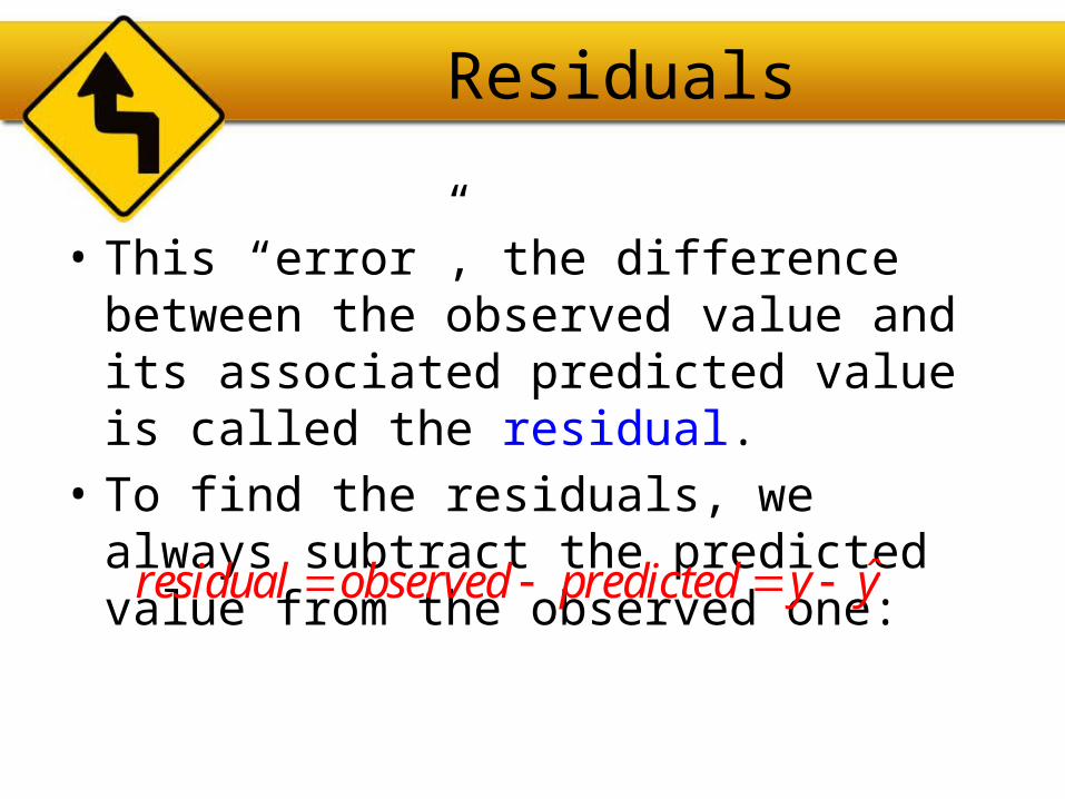
• This “error”, the difference between the observed value and its associated predicted value is called the residual.

• To find the residuals, we always subtract the predicted value from the observed one:

residual observed predicted y y

Residuals

• Symbol for residual is: e• Why e for residual?• Because r is already taken. No, the e stands for

“error.”• So, e y y

Residuals

• A negative residual means the predicted value’s too big (an overestimate).

• A positive residual means the predicted value’s too small (an underestimate).

• In the figure, the estimated fat of the BK Broiler chicken sandwich is 36 g, while the true value of fat is 25 g, so the residual is –11 g of fat.

“Best Fit” Means Least Squares

• Some residuals are positive, others are negative, and, on average, they cancel each other out.

• So, we can’t assess how well the line fits by adding up all the residuals.

• Similar to what we did with deviations, we square the residuals and add the squares.

• The smaller the sum, the better the fit.• The line of best fit is the line for which the sum of the

squared residuals is smallest, the least squares line.

16

Least – Squares Regression Line (LSRL)

• The LSRL is the line that minimizes the sum of the squared residuals between the observed and predicted y values (y – ŷ).

Correlation and the Line

• What we know about correlation from chapter 7 can lead us to the equation of the linear model.

• Start with a scatterplot of standardized values.

Original scatterplot - fat versus protein for 30 items on the Burger King menu.

Standardized scatterplot – zy (standardized fat) vs zx (standardized protein).


• What line would you choose to model the relationship of standardized values?

• Start at the center of the line. If an item has average protein , should it have average fat ?

• Yes, so the line should pass through the point . This is the first property of the line we are looking for, it must always pass through the point .

• In the plot of z-scores, the point is the origin and then the line passes through the origin (0, 0).

xy

,x y

,x y

,x y


• The equation for a line that passes through the origin is y = mx.

• So the equation on our standardized plot will be .

• We use to indicate that the point on the line is the predicted value , not the actual value zy.

y xz mz

yz

yz


• Many lines with different slopes pass through the origin. Which one best fits our data? That is, which slope determines the line that minimizes the sum of the squared residuals?

• It turns out that the best choice for slope is the correlation coefficient r.

• So, the equation of the linear model is .y xz rz


• • What does this tell us?• Moving one standard deviation

away from the mean in x moves us r standard deviations away from the mean in y.

• Put generally, moving any number of standard deviations away from the mean in x moves us r times that number of standard deviations away from the mean in y.

.y xz rz

How Big Can Predicted Values Get?

• • r cannot be bigger than 1 (in absolute value),

so each predicted y tends to be closer to its mean (in standard deviations) than its corresponding x was.

• This property of the linear model is called regression to the mean; the line is called the regression line.

.y xz rz

The Term Regression

• Sir Francis Galton related the heights of sons to the heights of their fathers with a regression line. The slope of the line was less than one.

• That is, sons of tall fathers were tall, but not as much above the mean height as their fathers had been above their mean. Sons of short fathers were short, but generally not as far from their mean as their fathers.

• Galton interpreted the slope correctly as indicating a “regression” toward the mean height. And regression stuck as a description of the method he used to find the line.

The Regression Line in Real Units

• Remember from Algebra that a straight line can be written as: • In Statistics we use a slightly different notation:

• We write to emphasize that the points that satisfy this equation are just our predicted values, not the actual data values.

• This model says that our predictions from our model follow a straight line.

• If the model is a good one, the data values will scatter closely around it.

y mx b

y b0 b1xy


• We write b1 and b0 for the slope and intercept of the line.

• b1 is the slope, which tells us how rapidly changes with respect to x.

• b0 is the y-intercept, which tells where the line crosses (intercepts) the y-axis.

y


• In our model, we have a slope (b1):– The slope is built from the correlation and the

standard deviations:

– Our slope is always in units of y per unit of x.

b1 rsy

sx


• In our model, we also have an intercept (b0).– The intercept is built from the means and the

slope:

– Our intercept is always in units of y.

b0 y b1x

Example: Fat Versus Protein

• The regression line for the Burger King data fits the data well:– The equation is

The predicted fat content for a BK Broiler chicken sandwich (with 30 g of protein) is 6.8 + 0.97(30) = 35.9 grams of fat.

6.8 0.97y x

Calculate Regression Line by Hand

• First calculate the following for the data;1. The means 2. The standard deviations 3. The correlation r

• Then the LSRL is

1. Slope

2. y- - intercept

30

Calculate Regression Line on TI-83/84

• Enter the data into lists: explanatory variable L1 and response L2

• STAT/CALC/LinReg(a+bx)/L1,L2,VARS/Y-VARS/FUNCTION/Y1

• Your display on the screen shows LinReg(a+bx)L1,L2,Y1.– This creates the LSRL and stores it as function Y1.– The LSRL will now overlay your scatterplot.

Graphing the LSRL by Hand

• The equation of the LSRL makes prediction easy. Just substitute an x-value into the equation and calculate the corresponding y-value.

• Use the equation to calculate two points on the line. One at each end of the line (ie. low x-value and high x-value).

• Plot the two points and draw a line.

Example: Calculate the LSRL by hand and on the calculator (r = -.64).

LSRL by Hand

• Calculate the slope

– From 2-VAR Stats

–

• Calculate the y-intercept– From 2-VAR Stats–

LSRL by Hand - Continued

• Then the LRSL is;–

• Or in the context of the problem–

35

By Calculator

• STAT/CALC/LinReg(a+bx)/L1,L2,VARS/Y-VARS/FUNCTION/Y1– y=a+bx– a=109.8738406– b=-1.126988915– r2=.4099712614– r=-.6402899823

• • or

Your Turn:

• Calculate the linear model by hand using r=.894.

• Solution: .0127 .018 or .0127 .018y x BAC Beers

37

Your Turn:

• Calculate and graph the linear model using the Ti-83/84.

• Solution:

Year Powerboat Reg. (1000s)

Manatees Killed

1977 447 13

1978 460 21

1979 481 24

1980 498 16

1981 513 24

1982 512 20

1983 526 15

1984 559 34

1985 585 33

1986 614 33

1987 645 39

1988 675 43

1989 711 50

1990 719 47

41.43 .125

41.43 .125 e .

y x

Manatees Killed Powerboat R g

Facts About LSRL

• The distinction between explanatory and response variables is essential in regression. LSR uses the distances of the data points from the line in only the y direction. If the 2 variables are reversed, you get a different LSRL.

• The LSRL always passes through the point .

More Facts on LSRL

• There is a close connection between correlation and the slope of the LSRL.

A change of one standard deviation in x corresponds to a change of r standard deviations in y.

Residuals Revisited

• The linear model assumes that the relationship between the two variables is a perfect straight line. The residuals are the part of the data that hasn’t been modeled.

Data = Model + Residual or (equivalently)

Residual = Data – ModelOr, in symbols, e y y

Residuals Revisited

• Residuals help us to see whether the model makes sense.

• When a regression model is appropriate, nothing interesting should be left behind.

• After we fit a regression model, we usually plot the residuals in the hope of finding…nothing.

Residuals Revisited

• The residuals for the BK menu regression look appropriately boring:

• The sum of the residuals is always equal to zero.

Finding Residuals

• Use the LSRL to find predicted values for each observed value and calculate the corresponding residual.

• Example:– Data – (0,1) (1,6) (2,8) (3,13) (4,13)– LSRL ŷ = 2 + 3.1x– e y y

Calculated Residuals

Residual Plot

• Is a scatterplot of the residuals against the explanatory variable (x).

• The residuals are plotted on the vertical axis.• The explanatory variable (x) is plotted on the

horizontal axis.• The residual plot helps us assess the fit of a

regression line.

Residual Plot

• Whenever you calculate a LSRL on the TI-83/84, the calculator automatically calculates the residuals for that particular LSRL and stores them in a list named RESIDS.

• To create a residual plot on the calculator, make sure you calculate the LSRL first.

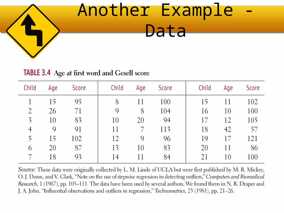
Another Example - Data

Scatterplot

Residual Plot

Your Turn:

• Plot the Residual Plot.

Year Powerboat Reg. (1000s)

Manatees Killed

1977 447 13

1978 460 21

1979 481 24

1980 498 16

1981 513 24

1982 512 20

1983 526 15

1984 559 34

1985 585 33

1986 614 33

1987 645 39

1988 675 43

1989 711 50

1990 719 47

What to Look for on the Residual Plot

• Random points, no pattern – data fits the linear model.

• Curved pattern – the relationship is not linear.

• Increasing (or decreasing) spread about the zero line as x increases – Prediction of y will be less (more) accurate for larger values of x.

Random Points, No Pattern

Curved Pattern

Increasing Spread

Residual Plot

• Individual points with large residuals – these points are outliers in the vertical (y) direction.

Outlier in they direction

Residual Plot

• Individual points that are extreme in the x direction – these points are outliers in the horiztonal (x) direction, such points may not have large residuals, but they can be very important.

Outlier in thex direction

Residual Plot

• No regression analysis is complete without a display of the residuals to check that the model is reasonable.

• Because the residuals are the “left over” after the model describes the relationship, they often reveal subtleties that were not clear from a plot of the original data.

Importance of Checking the Residual Plot

• The scatterplot of the data seems to indicate that a linear model will be a good fit.

Next, the LSRL

• The LSRL ŷ = 8.8 +7x yieds an r = .9992 and r2 = .9984.

Now the Residual Plot

• The residual plot, however, displays a distinctly curved pattern, indicating that a nonlinear model will be a better fit for the data.

• The pattern you see in the residual hints at a model you may need to fit your data.

Moral

• ALWAYS LOOK AT A RESIDUAL PLOT OF YOUR DATA!

• Any function is linear if plotted over a small enough interval.

• A residual plot will help you to see patterns in the data that may not be apparent in the original graph.

The Residual Standard Deviation

• If the residual plot shows no interesting pattern, we can look at how large the residuals are. After all, we are trying to make them as small as possible.

• Since the mean of the residuals is always zero, it makes sense to look at how they vary or their standard deviation.


• The standard deviation of the residuals, se, measures how much the points spread around the regression line.

• For se to make sense, the residuals should all share the same variation or spread.

• Check to make sure the residual plot has about the same amount of scatter throughout. Check the Equal Variance Assumption with the Does the Plot Thicken? Condition.

• We can check the Equal Variance Assumption in the original scatterplot or in the residual plot.

Equal Variance Assumption

• Use either the original scatterplot or the residual plot.

• Scatterplot: Variation about the regression line is about the same.• Residual plot: Variation about the zero residual line is about the same.• Therefore, both plots show the residuals meet the equal Variance

Assumption.


• We estimate the SD of the residuals using:

• We don’t need to subtract the mean because the mean of the residuals

• We divide by n-2 rather than n-1. We used n-1 for s when we estimated the mean (used for µ). Now we are estimating both slope and the y-intercept, so we use n-2. We subtract one more for each parameter we estimate.

se e2

n 2

e 0.

x


• Then it’s a good to make a histogram of the residuals.

• It should look unimodal and roughly symmetric.

• Then we can apply the 68-95-99.7 Rule to see how well the regression model describes the data.

R2—The Variation Accounted For

• The variation in the residuals is the key to assessing how well the model fits.

• Compare the variation ofthe response variable with the variation of the residuals.

• In the BK menu items example, total fat has a standard deviation of 16.4 grams. The standard deviation of the residuals is 9.2 grams.


• If the correlation were 1.0 and the model predicted the fat values perfectly, the residuals would all be zero and have no variation.

• As it is, the correlation is 0.83—not perfection.

• However, we do see that the model residuals had less variation than total fat alone.

• We can determine how much of the variation is accounted for by the model and how much is left in the residuals.


• The squared correlation, r2, gives the fraction of the data’s variance accounted for by the model.

• Thus, 1 – r2 is the fraction of the original variance left in the residuals.

• For the BK model, r2 = 0.832 = 0.69, so 31% of the variability in total fat has been left in the residuals.


• All regression analyses include this statistic, although by tradition, it is written R2 (pronounced “R-squared”). An R2 of 0 means that none of the variance in the data is in the model; all of it is still in the residuals.

• When interpreting a regression model you need to Tell what R2 means.– In the BK example, according to the model 69% of the

variation in total fat is accounted for by variation in the protein content.


• The R2 is the Coefficient of Determination, indicates how well the model (the LSRL) fits the data. R2 values are between 0 and 1. The closer R2 is to 1, the better the regression line explains the response. R2 gives the fraction of the variability of y that is explained by the least squares linear regression on x.

• Example: R2=.73 means 73% of the total variation in y is explained by the linear model.

How Big Should R2 Be?

• R2 is always between 0% and 100%. What makes a “good” R2 value depends on the kind of data you are analyzing and on what you want to do with it.

• The standard deviation of the residuals can give us more information about the usefulness of the regression by telling us how much scatter there is around the line.

Reporting R2

• Along with the slope and intercept for a regression, you should always report R2 so that readers can judge for themselves how successful the regression is at fitting the data.

• Statistics is about variation, and R2 measures the success of the regression model in terms of the fraction of the variation of y accounted for by the regression.

More on Outliers

• Outlying points can strongly influence regression.• A point can be an outlier because its x-value is

extraordinary, because its y-value is extraordinary, or because it deviates from the overall pattern of the data.

• A point has leverage and is call an influential point if its removal causes the slope of the regression line to change dramatically.

More on Outliers

• Although the indicated point lies outside the overall pattern of the data set, its removal has little effect on the regression line.

• It would not be considered an influential point.

More on Outliers

• The point in the lower right-hand corner of the graph is an outlier in the x-direction.

• Its removal causes the slope of the regression line to change dramatically.

• This point has leverage and is an influential point.

Influential Point - Summary

As seen in the prior examples, points that are outliers in the x-direction on a scatterplot are often influential on the calculation of the LSRL or linear model.

Regression: Assumptions and Conditions

• Quantitative Variables Condition:– Regression can only be done on two quantitative

variables (and not two categorical variables), so make sure to check this condition.

• Straight Enough Condition:– The linear model assumes that the relationship

between the variables is linear. – A scatterplot will let you check that the

assumption is reasonable.


• If the scatterplot is not straight enough, stop here. – You can’t use a linear model for any two variables,

even if they are related. – They must have a linear association or the model

won’t mean a thing.• Some nonlinear relationships can be saved by

re-expressing the data to make the scatterplot more linear.


• It’s a good idea to check linearity again after computing the regression when we can examine the residuals.

• Does the Plot Thicken? Condition: – Look at the residual plot -- for the standard

deviation of the residuals to summarize the scatter, the residuals should share the same spread. Check for changing spread in the residual scatterplot.


• Outlier Condition: – Watch out for outliers. – Outlying points can dramatically change a

regression model.– Outliers can even change the sign of the slope,

misleading us about the underlying relationship between the variables.

• If the data seem to clump or cluster in the scatterplot, that could be a sign of trouble worth looking into further.

Reality Check: Is the Regression Reasonable?

• Statistics don’t come out of nowhere. They are based on data. – The results of a statistical analysis should reinforce

your common sense, not fly in its face. – If the results are surprising, then either you’ve

learned something new about the world or your analysis is wrong.

• When you perform a regression, think about the coefficients and ask yourself whether they make sense.

What Can Go Wrong?

• Don’t fit a straight line to a nonlinear relationship.• Beware extraordinary points (y-values that stand off

from the linear pattern or extreme x-values).• Don’t extrapolate beyond the data—the linear model

may no longer hold outside of the range of the data.• Don’t infer that x causes y just because there is a

good linear model for their relationship—association is not causation.

• Don’t choose a model based on R2 alone.

What have we learned?

• When the relationship between two quantitative variables is fairly straight, a linear model can help summarize that relationship.– The regression line doesn’t pass through all the

points, but it is the best compromise in the sense that it has the smallest sum of squared residuals.


• The correlation tells us several things about the regression:– The slope of the line is based on the correlation,

adjusted for the units of x and y.– For each SD in x that we are away from the x mean, we

expect to be r SDs in y away from the y mean.– Since r is always between –1 and +1, each predicted y

is fewer SDs away from its mean than the corresponding x was (regression to the mean).

– R2 gives us the fraction of the response accounted for by the regression model.


• The residuals also reveal how well the model works.– If a plot of the residuals against predicted values

shows a pattern, we should re-examine the data to see why.

– The standard deviation of the residuals quantifies the amount of scatter around the line.


• The linear model makes no sense unless the Linear Relationship Assumption is satisfied.

• Also, we need to check the Straight Enough Condition and Outlier Condition with a scatterplot.

• For the standard deviation of the residuals, we must make the Equal Variance Assumption. We check it by looking at both the original scatterplot and the residual plot for Does the Plot Thicken? Condition.

REVIEWPut it Altogether Example

Example: Creating and Using a Least Squares Regression Line

A student wanted to see how good she was at predicting distances measured in meters. She randomly selected 7 distances to estimate. After recording her estimated distances, she used a range finder to find the actual distances. Next is a scatterplot of the Actual Distances vs. Estimated Distances and the corresponding residual plot.

Make a Picture

Check Conditions for Regression

• Quantitative Variables Condition: Actual Distance and Estimated Distance are quantitative.

• Straight Enough Condition: The data follow a straight line pattern.

• Outlier Condition: There are no outliers in the data.• Does the Plot Thicken? Condition: The residual plot

shows no obvious patterns.• The scatterplot follows a linear pattern with no

apparent outliers. The residual plot shows no discernable pattern, so a linear model is appropriate.

Numerical Analysis

• Use your calculator to find the equation of the LSRL, if given the data; however, you need to be able to read various computer outputs to be successful on the AP Statistics exam.

There will be things on the printout that you might not be familiar with, such as the F-ratio. Focus on finding the information you need to write the equation of the LSRL (ie. Slope & y-intercept).

Typical Questions on the Regression

• State the equation of the LSRL. Define any variables used.

Answer

• The equation of the LSRL is = 0.1322 + 0.9203(estimated distance)

or ŷ = 0.1322 + 0.9203x, where x=estimated distance & ŷ=actual distance

Question

• Interpret the slope and the y-intercept of the LSRL.

Answer

In the context of the problem:For every additional meter of estimated distance, the predicted actual distance increases by approximately 0.92 meters. (remember, all interpretations must be given in context).

Continued

• The y-intercept of is the predicted value of y when x is equal to zero.

• = 0.1322 = 0.9203 (0) = 0.1322• In the context of the problem:

A y-intercept of 0.1322 represents the predicted distance in meters when the distance between the person and the object being measured is zero – the person is holding the object. This value does not make sense in the context of this problem since a person holding an object would not make a prediction other than zero.

Question

• State and interpret the correlation coefficient.

Answer

• The correlation coefficient is r, and since we are given that R2 = 91.2% or 0.912, then (r is positive because the slope is positive).

• The correlation coefficient indicates that there is a strong, positive, linear relationship between the estimated distance and the predicted actual measured distance.

Question

• State and interpret the coefficient of determination.

Answer

• The coefficient of determination, R2 = .912.• Tells us that approximately 91% of the

variability in the actual distance can be explained by a linear relationship between the actual distance and the estimated distance.

Question

• Predict the actual distance from an object when the estimated distance is 4 meters.

Answer

• = 0.1322 + 0.9203 (4) = 3.8 • The Linear model predicts that an estimated

distance of 4 meters will correspond to a predicted actual distance of 3.8 meters.

Question

• For an estimated distance of 4 meters, the actual distance from the object was 4.2 meters. What is the residual for this data value?

Answer

• Residual = observed – predicted or • Residual = 4.2 – 3.8 = 0.4 meters

e y y

Assignment

• Ch-8 pg 192 – 199: 2, 3, 7 -12, 17, 18, 22, 25, 31, 32, 41, 49

Documents

AP Statistics Chapter 8 Linear Regression. Objectives: Linear model Predicted value Residuals Least squares Regression to the mean Regression line Line