APM 541: Population Genetics Models - Arizona State …jtaylor/teaching/Fall2013/APM541/lectures/...Population Genetics Jay Taylor Fall 2013 ... Genetic variation is the raw material

;

APM 541: Stochastic Modelling in BiologyPopulation Genetics

Jay TaylorFall 2013

Jay Taylor (ASU) APM 541 Fall 2013 1 / 41

Motivation

The central aim of population genetics is to understand the causes andconsequences of genetic variation . . .

polymorphism within populations

(Durbin et al., 2010)

divergence between populations

(Gilbert, 2007)


Motivation

Why study genetic variation?

Genetic variation is the raw material of evolution. To understand how species ariseand adapt to their environments, we need to understand genetic variation and itsrelationship to phenotypic differences.

Genetic variation can be used to infer demographic history and populationstructure. Human genetic variation strongly supports a sub-Saharan African originfor our species, followed by a colonization of the Near East some 100,000 yearsago and subsequent migrations into Europe and Asia (∼ 40-50 kya). However,there is also growing evidence of admixture between modern and archaic humans,including Neanderthals and Denisovans.

Genetic variation is increasingly relevant to medicine. Genome-wide associationstudies can be used to identify mutations associated with disease phenotypes,which in turn can be used to assess risk and to design individualized treatments.


Motivation

Variation is influenced both by molecular and by demographic processes.

Mutation and recombination tend to increase variation by creating newgenotypes and sometimes re-creating old genotypes that have been lost.

Natural selection alters the genetic composition of populations and can either

reduce or increase variation depending on its mode of action.

Purifying selection tends to reduce variation.In some cases, balancing selection and diversifying selection can act tomaintain variation.

Genetic drift (demographic stochasticity) tends to reduce genetic variationthrough the random loss of rare alleles.

Migration can increase local levels of variation.

One of the challenges to understanding evolution and biodiversity is that these dependon processes that occur on spatial and temporal scales spanning many orders ofmagnitude.


Motivation

Wing color variation in the scarlet tiger moth (Callimorpha dominula) is controlled by asimple Mendelian polymorphism. However, the genetic composition of the Cothill Fenpopulation in the UK changed substantially between 1939 and 1979 (O’Hara, 2005).

Estimated frequency of the medionigra morph in the Cothill scarlet tiger moth population

0

0.02

0.04

0.06

0.08

0.1

0.12

1935 1940 1945 1950 1955 1960 1965 1970 1975 1980

year

freq

uen

cy


Genetic Drift: Moran Model

The Moran Model

Assumptions:

The population size is constant, with N haploid individuals.

Two alleles, A1 and A2, are present in the population.

For now, we will ignore mutation.

Likewise, we will also assume that all individuals have the same fitness, i.e.,reproduction and mortality do not depend on an individual’s genotype. When thislatter condition holds, we say that the two alleles are neutral.

Births and deaths occur continuously throughout the year. Specifically, at eachtime step, one of the N individuals is chosen uniformly at random and gives birthto a single offspring. A second individual is then chosen uniformly at random anddies.

This model was introduced by P. A. P. Moran in 1954 and is one of the mostwidely-studied processes in population genetics.



Let Yt denote the number of copies of the A1 allele contained in the population at timet. Then Yt takes values in the set E = {0, 1, · · · ,N} and Yt+1 and Yt differ by at mostone.

The number of copies of A1 will increase by 1 if an A1 individual reproduces andan A2 individual dies.

The number of copies will decrease by 1 if an A2 individual reproduces while an A1

individual dies.

The number of copies will stay the same if the individual that gives birth and theindividual that dies have the same genotype.

This shows that Y = (Yt : t ≥ 0) is a birth-death process with the following transitionprobabilities:

P (Yt+1 = j |Yt = k) =

8<:p(1− p) if j = k − 1 or k + 11− 2p(1− p) if j = k0 otherwise,

where p = k/n is the frequency of allele A1 in the population.



Units

Frequencies: Since the population sizes of most species are unknown, the Moran modelis usually formulated in terms of the allele frequencies:

Xt =1

NYt .

Here X = (Xt : t ≥ 0) is itself a birth-death process, but it takes values in the space{0, 1/N, · · · , 1}. This is useful because we can often estimate allele frequencies (bygenotyping samples of individuals) even when we are unable to directly estimate N.

Time scale: We should also consider the time scale of this process. Here time ismeasured in units such that there is one birth and one death event per time step. Sinceit will be convenient to convert to a generational time scale for comparison with othermodels, we note that the generation time for the Moran model is N time steps. To seethis, note that each individual has probability 1/N of dying per time step. Thus the lifespan of each individual is geometrically distributed, with parameter 1/N, and the meanof this distribution is N.



Because 0 and N are the only absorbing states for this model, the ultimate fate of alleleA1 is either to be lost from the population (p = 0) or to rise in frequency until it is theonly allele remaining at that locus (p = 1). In the latter case, we say that the allele hasbeen fixed in the population. An important quantity in population genetics is thefixation probability of an allele, which depends on its initial frequency and is defined as

u(p) ≡ Pp(Xt = 1 for some t > 0|X0 = p).

Since this is the same as the probability of absorption at 1 given the initial frequency p,we know that the quantities u(p) satisfy the following system of linear equations:

u(0) = 0

u(1) = 1

u(p) = p(1− p)u(p − 1/N) + (1− 2p(1− p))u(p) + p(1− p)u(p + 1/N).



By subtracting u(p) from both sides and then dividing by p(1− p), this last equationcan be rewritten as

0 = u(p − 1/N)− 2u(p) + u(p + 1/N)

which has the general solution

u(p) = Ap + C

where A and C are constants. In this case, we know that u(0) = 0 and u(1) = 1, whichshows that u(p) = p. Thus

The fixation probability of a neutral allele is equal to its initial frequency.

In particular, the fixation probability of a new neutral mutation is just 1/N.



Another quantity of interest is the mean time until one of the two alleles is fixed in thepopulation. This also depends on the initial frequency and so we define

Tfix ≡ inf{t > 0 : Xt = 0 or Xt = 1}τi ≡ E[Tfix |X0 = i/N].

Since absorption at one or the other boundary is certain to occur, we know that thevector of mean absorption times (τ0, τ1, · · · , τN ) is a solution to the system of linearequations

τi = 1 + pi (1− pi )(τi−1 + τi+1) + (1− 2pi (1− pi ))τi

with pi = i/N and τ0 = τN = 0. This can be rearranged into a more accommodatingform:

τi−1 − 2τi + τi+1 = −N

„1

i+

1

N − i

«.



This system of equations is essentially a discrete one-dimensional version of Poisson’sequation ∆φ = −ρ and has the following general solution

τi = a + b · i − Ni−1Xk=1

(i − k)

„1

k+

1

N − k

«,

where a and b are constants that must be chosen so that the boundary conditions aresatisfied. This leads to the following solution:

τi = N

"(N − i)

i−1Xk=1

1

N − k+ i

N−1Xk=i

1

k

#.



Although this last result is exact, a somewhat more telling expression can be derived byapproximating the two sums by integrals:

i−1Xk=1

1

N − k≈

Z pi

0

dq

1− q= − ln(1− pi )

N−1Xk=i

1

k≈

Z 1

pi

dq

q= − ln(pi ),

which gives the striking result:

τi ≈ N2˘− pi ln(pi )− (1− pi ) ln(1− pi )¯.



We can draw the following conclusions from these results:

Provided that neither allele is very rare (i.e., 0� p � 1), the mean time until oneof the two alleles is lost from the population is of order O(N2) events or(equivalently) order O(N) generations.

This suggests that larger populations will retain polymorphism for longer timesthan smaller populations.

Nonetheless, in the absence of processes that create new variation, the ultimatefate of the population will be to lose all neutral polymorphism.

A fair question is whether these results hold (at least qualitatively) in other models ofgenetic drift.


Genetic Drift: Wright-Fisher Model

The Wright-Fisher Model

Assumptions:

The population size is constant, with N haploid individuals.

Two alleles, A1 and A2, are present in the population.

As above, we will continue to ignore mutation and assume that all individuals havethe same fitness.

The main difference is that we will consider a population with non-overlappinggenerations, in which individuals survive for exactly one generation, reproduce, andthen die (e.g., mayflies, annual plants).

Each individual alive in generation t + 1 independently chooses its parent from thepreceding generation uniformly at random and with replacement.

Intuition: Each parent gives birth to a large number of offspring, but only N offspringsurvive to form the next generation.



Multinomial Sampling in the Wright-Fisher Model



If Yt denotes the number of A1 alleles present in generation t, then conditional onYt = i , the distribution of Yt+1 is

Yt+1 ∼ Binomial(N, i/N).

Thus the entries of the transition matrix for the Markov chain Y = (Yt : t ≥ 0) are

pij =

N

j

!„i

N

«j „1− i

N

«N−j

.

However, as with the Moran model, we will prefer to work with the frequency processdefined by setting Xt = Yt/N.



Using the properties of the binomial distribution, we can show that:

Ep[X1] = p

Ep[(X1 − p)2] =p(1− p)

N

Remarks:

The average frequencies of the alleles do not change between generations.

However, the actual frequencies do fluctuate and the variance of these fluctuationsis inversely proportional to population size. Thus, genetic drift is more pronouncedin small populations than in large populations.

This model is easy to describe and simulate, but because almost all of the entriesin the transition matrix are positive, very few exact analytical results are knownexcept for very small values of N.



Simulations of the Neutral Wright-Fisher Model

0 10 20 30 40 50 60 70 80 90 1000

0.1

0.2

0.3

0.4

0.5

0.6

0.7

0.8

0.9

1Neutral Wright−Fishermodel

Generation

p

N = 100

0 10 20 30 40 50 60 70 80 90 1000

0.1

0.2

0.3

0.4

0.5

0.6

0.7

0.8

0.9


Generation

p

N = 1000



One quantity that we can calculate exactly is the fixation probability of A1 as a functionof its initial frequency. (Note that p = 0 and p = 1 are still absorbing states.) Onceagain denoting this probability as

u(x) ≡ Px (Xt = 1 for some t > 0).

we know that the quantities u(p) satisfy the following system of linear equations:

u(0) = 0

u(1) = 1

u(p) =NX

j=0

N

j

!pj (1− p)N−ju(j/N)

for p ∈ {1/N, 2/N, · · · , 1− 1/N}.



While these equations do not lead to a useful recursion, the last identity can berewritten in the following form

u(p) = Ep[u(X1)].

Fortunately, we have already noticed that

p = Ep[X1]

for all p ∈ {0, 1/N, · · · , 1}, and comparing these two equations leads us to the solutionu(p) = p. Thus, as in the Moran model,

The fixation probability of a neutral allele in the Wright-Fisher model is equal tothe initial frequency of that allele.

Furthermore, this result holds in a much larger class of neutral population geneticsmodels which include the Moran and Wright-Fisher models as special cases.Essentially, it is a consequence of the fact that each individual alive in anyparticular generation is equally likely to be the one individual from which the entirepopulation is descended in some future generation.



We next turn our attention to the mean time to fixation of one of the two alleles, whichwe again denote

τi = E[Tfix |X0 = pi ]

where pi ≡ i/N. We know that these quantities satisfy the following system of equations

τi = 1 +NX

j=0

N

j

!pj

i (1− pi )N−jτj ,

with τ0 = τN = 0. Unfortunately, there is little hope of solving these equations exactlyand so we need a new approach. We begin by observing that when N is large, thedifference τi+1 − τi is likely to be small, at least in comparison with τi itself. Thissuggests that we write

τi = τ(i/N)

where τ(p) is a continuous function. In fact, we will be extremely bold and suppose thatτ is a smooth function on (0, 1).



With these assumptions, if we fix a value of i and let δj ≡ pj − pi , then by expandingτ(pj ) in a Taylor series around pi , we can rewrite the previous equation as:

τ(pi ) = 1 +NX

j=0

N

j

!pj

i (1− pi )N−j τ (pi + δj )

≈ 1 +NX

j=0

N

j

!pj

i (1− pi )N−j

„τ(pi ) + τ ′(pi )δj +

1

2τ ′′(pi )δ

2j + O

“|δj |3

”«

= 1 + τ(pi ) + τ ′(pi )1

N

(NX

j=0

N

j

!pj

i (1− pi )N−j (j − i)

)+

1

2N2τ ′′(pi )

(NX

j=0

N

j

!pj

i (1− pi )N−j (j − i)2

)+

1

N3R(pi )

(NX

j=0

N

j

!pj

i (1− pi )N−j (j − i)3

)

where R(pi ) is some bounded function of pi .



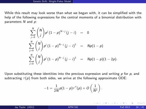
While this result may look worse than what we began with, it can be simplified with thehelp of the following expressions for the central moments of a binomial distribution withparameters N and p:

NXj=0

N

j

!pj (1− p)N−j (j − i) = 0

NXj=0

N

j

!pj (1− p)N−j (j − i)2 = Np(1− p)

NXj=0

N

j

!pj (1− p)N−j (j − i)3 = Np(1− p)(1− 2p).

Upon substituting these identities into the previous expression and writing p for pi andsubtracting τ(p) from both sides, we arrive at the following approximate ODE:

−1 =1

2Np(1− p)τ ′′(p) + O

„1

N2

«.



Assuming that the higher-order terms can be dropped when N is large, we arrive at thefollowing boundary-value problem:

τ ′′(p) = − 2N

p(1− p)= −2N

„1

p+

1

1− p

«with τ(0) = τ(1) = 0. This has a unique solution,

τ(p) = 2N˘− p ln(p)− (1− p) ln(1− p)

¯,

where time is measured in units of generations.



Let us compare the mean fixation time for the Wright-Fisher model with the quantitythat we derived for the Moran model. When N is large, these times are

τFW (p) ≈ 2N˘− p ln(p)− (1− p) ln(1− p)

¯τMoran(p) ≈ N

˘− p ln(p)− (1− p) ln(1− p)

¯and so we see that the two expressions are nearly identical apart from a factor of 2, i.e.,on average, it takes twice as long for one of the alleles be fixed in the Wright-Fishermodel as it does in the Moran model.

To understand why genetic variation is lost twice as rapidly in the Moran model as inthe Wright-Fisher model, we need to consider the variance of the number of offspringborn to individuals in each model.



First consider the Wright-Fisher model and suppose that we label the individuals1, · · · ,N. If we let ηi denote the number of surviving offspring that the i ’th individualcontributes to the next generation, then ηi is binomially distributed with parameters Nand 1/N

P(ηi = k) =

N

k

!„1

N

«k „1− 1

N

«N−k

for k = 0, · · · ,N. In particular, the mean and the variance of the number of offspringcontributed by this individual are:

E[ηi ] = 1

Var(ηi ) = N

„1

N

«„1− 1

N

«=

„1

N

«,

which is approximately 1 when N is large.



To determine the mean and the variance of the number of offspring contributed by anindividual in the Moran model, we consider the following quantities:

First, the lifespan of an individual is a random variable T which is geometricallydistributed with parameter 1/N.

In each of these T time steps, this individual has probability 1/N of reproducing,in which case they will contribute exactly one new offspring.

If we let B1, · · · ,BT denote the numbers of offspring contributed by this individualin each of the T time steps of their life, then these Bi ’s are i.i.d. Bernoulli randomvariables, each with parameter 1/N.

Putting these results together, the total number of offspring contributed by thisindividual is given by the following random sum:

η ≡ B1 + · · ·+ BT =TX

i=1

Bi .



The mean and the variance of η can be calculated with the help of Wald’s identities:

E[η] = ET · EB1 = N · 1

N= 1

Var(η) = ET · Var(B1) + (EB1)2 · Var(T )

= N · 1

N

„1− 1

N

«+

„1

N

«21− 1/N

1/N2

= 2

„1− 1

N

«,

which is approximately 2 when N is large. Thus, although the mean number of offspringcontributed by an individual is the same in both models, the variance in this number istwice as great in the Moran model as it is in the Wright-Fisher model. The connectionwith the mean fixation times in these two models is explained on the next slide.



Genetic Drift and Fecundity Variance

Genetic drift - the random fluctuation in allele frequencies - is a direct consequenceof the random variation in reproductive success between individuals. Sometimes anallele will increase in frequency, not because it confers a fitness advantage, butbecause the individuals carrying that allele by chance contributed more offspring.

As a general rule, the larger the population, the weaker genetic drift will be. Thisis because each individual’s reproductive output is (nearly) independent of that theothers and so random variation in this output will tend to be averaged out in alarge population.

On the other hand, genetic drift will be stronger in populations where there islarge reproductive variance between individuals.

In a large populations, the mean fixation time is approximately inverselyproportional to the variance in the number of offspring contributed by anindividual:

Ep[Tfix ] ≈ 2N

Var(η)

˘− p ln(p)− (1− p) ln(1− p)

¯


Mutation-Drift Balance


In our initial studies of the Moran and Wright-Fisher models, we made thesimplifying assumption that we could ignore mutation so that we could emphasizethe effects of genetic drift on an initially polymorphic population.

Since single nucleotide mutation rates are on the order of 10−8 mutations per siteper generation in many Eukaryotes, this is not an unreasonable assumptionprovided that the population is not too large and that we focus on relatively shorttime scales.

However, in large populations or over long time scales, a given site will mutaterepeatedly. In these cases, the focus is not so much on fixation probabilities, buton the equilibrium distribution of allele frequencies under the opposing forces ofmutation and genetic drift. Since mutation creates variation, while genetic driftreduces it, the amount of polymorphism in a population will be maintained atsome intermediate level depending on the relative strengths of these two processes.



To investigate this question, we will modify the Moran model introduced earlier so thatit includes mutation. Specifically, we will modify our earlier assumptions by stipulatingthat:

Whenever an A1 individual gives birth, with probability µ, their offspring willinherit the A2 allele (i.e., they will be mutant). Otherwise, the offspring will inheritthe A1 allele.

Similarly, whenever an A2 individual gives birth, with probability ν, their offspringwill inherit the A1 allele. Otherwise, the offspring will inherit the A2 allele.

In all other respects, our new model will coincide with the original. In particular, we willcontinue to assume that the two alleles are neutral.



With theses changes, the transition probabilities now take the following form

P (Yt+1 = j |Yt = k) =

8>><>>:(1− µ)p(1− p) + ν(1− p)2 if j = k + 1(1− ν)p(1− p) + µp2 if j = k − 11− 2p(1− p)− ν(1− p)2 − µp2 if j = k0 otherwise,

where p = k/N. As in the original model, the number of A1 alleles can only change by asingle copy in each time step, so that this modified model is still a birth-death process.On the other hand, p = 0 and p = 1 are no longer absorbing states for the frequencyprocess Xt = Yt/N and indeed both X and Y are now irreducible, aperiodic Markovchains with finite state spaces. From previous theory, we know that this means that Xhas a unique stationary distribution, which we will now identify.



To apply our results on the stationary distribution of an irreducible birth-death process,we need to specify the birth and death rates for the modified Moran model. These canbe written as:

bk =k(N − k)

N2(1− µ) +

„N − k

N

«2

ν

dk =k(N − k)

N2(1− ν) +

„k

N

«2

µ,

with ratio

bk

dk=

1 +“ν 1−k/N

k/N− µ

”1 +

“µ k/N

1−k/N− ν” ≈ 1 +

ν

k/N− µ

1− k/N,

where the second expressions holds when µ and ν are small enough to ignore expressionsof order µ2 and ν2. For single nucleotide mutation rates, this approximation is quiteaccurate.



With these expressions, the stationary distribution for the Moran model with mutationcan be written as:

π0 =

1 +

NXk=1

b0 · · · bk−1

d1 · · · dk

!−1

≈

1 +

NXk=1

ν

dk

k−1Yj=1

„1 +

ν

j/N− µ

1− j/N

«!−1

πk =

„b0 · · · bk−1

d1 · · · dk

«π0

≈ π0ν

dk

k−1Yj=1

„1 +

ν

j/N− µ

1− j/N

«,

where k = 1, · · · ,N.



If we assume that N is large and we write µ = θa/N and ν = θA/N, where θa and θA aresmall in comparison with N, then the stationary distribution can be further simplified.Let pk ≡ k/N. Then

k−1Yj=1

„1 +

ν

j/N− µ

1− j/N

«= exp

(log

k−1Yj=1

„1 +

ν

j/N− µ

1− j/N

«!)

= exp

(k−1Xj=1

log

„1 +

ν

j/N− µ

1− j/N

«)

≈ exp

(1

N

k−1Xj=1

„Nν

pj− Nµ

1− pj

«)

≈ exp

(Z pk

1/N

„θA

p− θa

1− p

«dp

)= exp {θA ln(pk ) + θa ln(1− pk ) + C}= CpθA

k (1− pk )θa ,

where C is a constant that does not depend on k.



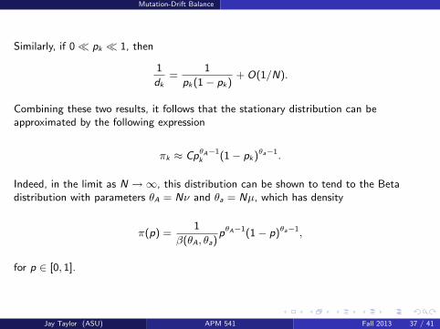
Similarly, if 0� pk � 1, then

1

dk=

1

pk (1− pk )+ O(1/N).

Combining these two results, it follows that the stationary distribution can beapproximated by the following expression

πk ≈ CpθA−1k (1− pk )θa−1.

Indeed, in the limit as N →∞, this distribution can be shown to tend to the Betadistribution with parameters θA = Nν and θa = Nµ, which has density

π(p) =1

β(θA, θa)pθA−1(1− p)θa−1,

for p ∈ [0, 1].



The stationary distribution reflects the competing effects of genetic drift, whicheliminates variation, and mutation, which generates variation.

0 0.1 0.2 0.3 0.4 0.5 0.6 0.7 0.8 0.9 10

1

2

3

4

5

6

7

8

p

density

StationaryDistribution of the MoranModel

Nµ=0.02

Nµ=0.2

Nµ=2.0

When Nµ1,Nµ2 > 1, mutation dominates drift and the stationary distribution ispeaked about its mean (both alleles are common).

When Nµ1,Nµ2 < 1, drift dominates mutation and the stationary distribution isbimodal, with peaks at the boundaries (one allele is common and one rare).



Simulations of the Neutral Moran Model with Mutation

0 1 2 3 4 5 6 7 8 9 10

x104

0

0.1

0.2

0.3

0.4

0.5

0.6

0.7

0.8

0.9


Generation

p

N = 1000, µ = 10−4

0 1 2 3 4 5 6 7 8 9 10

x104

0

0.1

0.2

0.3

0.4

0.5

0.6

0.7

0.8

0.9


Generation

p

N = 10000, µ = 10−4



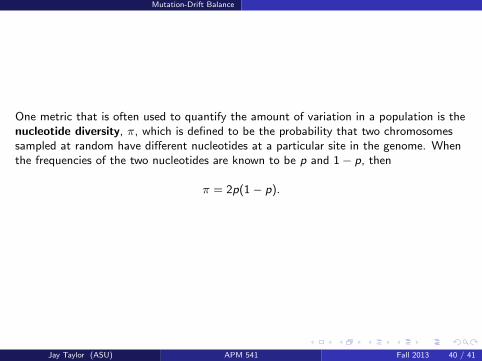
One metric that is often used to quantify the amount of variation in a population is thenucleotide diversity, π, which is defined to be the probability that two chromosomessampled at random have different nucleotides at a particular site in the genome. Whenthe frequencies of the two nucleotides are known to be p and 1− p, then

π = 2p(1− p).



In a population at equilibrium, p will be distributed according to the Beta distributionand then we can characterize the amount of variation maintained in the populationusing the average of the nucleotide diversity with respect to this distribution:

π =

Z2p(1− p)

1

β(θA, θa)pθA−1(1− p)θa−1dp

= 2β(θA + 1, θa + 1)

β(θA, θa)

=2θAθa

(θA + θa)(1 + θA + θa)

=θ

1 + 2θif θA = θa = θ.

Thus, when θ = Nµ is small, we are very unlikely to sample two individuals that carrydifferent nucleotides at a particular site. For the global human population, estimates ofθ using non-coding sequences are mostly around 0.001, with roughly one in every 1000sites differing between any two randomly sampled individuals.


Documents

APM 541: Population Genetics Models - Arizona State …jtaylor/teaching/Fall2013/APM541/lectures/...Population Genetics Jay Taylor Fall 2013 ... Genetic variation is the raw material