APOGEE:The Apache Point Observatory Galactic Evolution Experiment l

M. P. Ruffoni1, J. C. Pickering1, E. Den Hartog2, G. Nave3, J. Lawler2, C. Allende-Prieto4

1.Imperial College London, UK

2.University of Wisconsin, Madison, WI, USA

3.NIST, Gaithersburg, MD, USA

4.University of Texas, Austin, TX, USA

1

Duration Spring 2011 to Summer 2014

Spectra Measuring 1.51µm < < 1.7µmResolving power ~30,000S/N Ratio greater than 100

Targets 100,000 evolved stars

15 elements - Fe most important

Precision Metal abundances to ~0.1 dexRadial velocities to <0.3 km s-12

APOGEE is one of 4 instruments formingthe third Sloan Digital Sky Survey (SDSS3)

It will conduct a spectroscopic survey of all stellar populations in the Milky Way

It will measure in the near-IR where Galactic dust extinction is ~1/6 of that at visible wavelengths

It will measure chemical abundances and radial velocities of 100,000 evolved stars to help explain Galactic evolution

Detecting elements in stars

Photosphere

Hot, denseinterior

Emission contains absorption lines

Section of a star

Visible spectra for different star types

n = E = 0n = 4 E = -0.85 eVn = 3 E = -1.51 eV

n = 2 E = -3.40 eV

n = 1 E = -13.6 eV

Type

Absorption lines indicate the presence of an element.

Line strength is mainly linked to:

•Stellar properties (e.g. temperature)•Absorption transition probability•Chemical abundance

Temperature/KType

K A O

Effect of lower level population on H

3

Why look at QSOs when studying ?

Determining chemical abundances

1) Use a 2 fit to stellar models to find• Stellar temperature• Surface gravity• Microturbulence parameter• Abundance of important elements

[Fe/H], [C/H], and [O/H]

2) Fix these parameters then fit other abundances

Simulated H-band spectra for an Fe-poor (black) and Fe-rich (grey) star. All other parameters fixed.

4

Experimentally measured transition probabilities in the literature:

J. C. Pickering et al. Can J Phys 89 pp. 387 (2011)

Sc Ti V Cr Mn Fe Co Ni Cu Zn

– 45 7 – 26 51 – 4 – 1

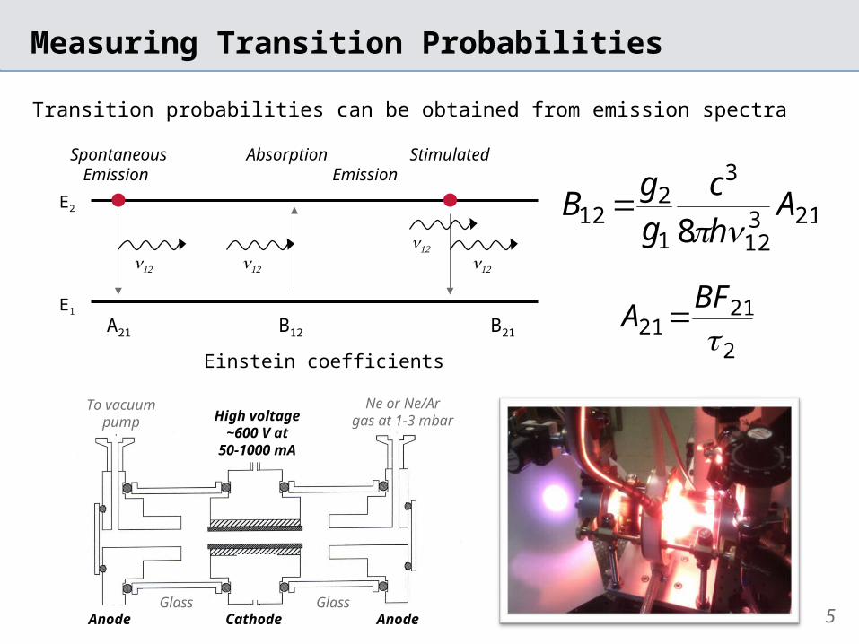
Measuring Transition Probabilities

E2

E1

11

1

1

A21 B12 B21

Einstein coefficients

Spontaneous Absorption Stimulated Emission Emission

21312

3

1

212

8A

h

cgg

B

Transition probabilities can be obtained from emission spectra

2

2121

BFA

5

To vacuumpump High voltage

~600 V at50-1000 mA

Ne or Ne/Argas at 1-3 mbar

Glass GlassAnode Cathode Anode

Decay to a single level

Decay to multiple levels

E2

E1

E2

E1

I I

I

I

12

Branching Fractions

i iEWEW

BF2

2121

2

2121

BFA

12

12 12

BF = Branching fractionEW = Line equivalent width

6

Free spectral range

Spectral range determined by

• Spectrometer optics• Detector sensitivity• Filter combinations• Measurement electronics

Complications

1.0

0.0

Spectrometer Response

Determined by measuring a calibrated continuum source

• Tungsten lamp (IR to UV)• Deuterium lamp (UV and vacuum UV)

I

1.0

0.0

I

Norm

alis

ed

re

spon

se

0 4000 8000 12000 35000 45000 55000Wavenumber / cm-1

1.0

0.8

0.6

0.4

0.2

0.0Norm

alis

ed

Resp

on

se

W lamp D2 Lamp

Either

Select a range to measureall upper level branches

or

Use overlapping spectrato carry calibration

7

Branching Fractions for APOGEE

A21 for Neutral Fe (Fe I) is of the greatest importance

Wavenumber / cm-1

S/N

S/N

x C

alib

rati

on f

unct

ion

/ cm-1 EW BF / %

6124.10169 2413.49953 7 ± 3

6395.40329 10599.58897 32 ± 2

6742.87349 19624.82794 60 ± 2

• Target H-band lines in a single spectral range

• Extract all lines from a single upper level

• Calibrate line intensities

• Fit line profiles to get BFs

8

Catch-22: Branching fractions or level lifetimes

Laser induced fluorescence (LIF) is used to measure 2

E2

E1

205 - 720 nmUV - visible

No significantly populated lower level to excite

Not possible to measure 2

0 4000 8000 12000 35000 45000 55000Wavenumber / cm-1

1.0

0.8

0.6

0.4

0.2

0.0Norm

alis

ed

Resp

on

se

Change target levels so they are LIF compatible

No lines to carry calibration

Not possible to measure BFs

9

Solutions

Some levels contain visible lines to link IR spectra to UV spectra

• LIF has a low lying level available• FTS line intensities can be calibrated

For FTS compatible upper levels

• Use theory to calculate 2 (check against known levels)• Constrain models with stellar spectra

For LIF compatible upper levels

• Use lines from similar upper levels as calibration proxies• Link spectral regions with theory calculations• Use stellar spectra to estimate missing calibration factors

The work continues ... (with the support of the STFC)

10