Appendices for: Conducting Ecological Risk Assessments

Oregon Department of Environmental Quality

Appendices for: Conducting Ecological Risk Assessments

Land Quality Division Cleanup Program 700 NE Multnomah St. Suite 600 Portland, OR 97232 Phone: 503-229-5696

800-452-4011 Fax: 503-229-6124 Contact: Jessika Cohen

DEQ is a leader in restoring, maintaining and enhancing the quality of Oregon’s air, land and water.

Oregon Department of Environmental Quality ii

DEQ can provide documents in an alternate format or in a language other than English upon request. Call DEQ at 800-452-4011 or email [email protected].

mailto:[email protected]

Oregon Department of Environmental Quality 1

Appendix A1: Basic Site Information Checklist


General Site Information

ECSI File No. or LUST File No.:

Site Name:

Site Location (address, city, and/or county):

Latitude/Longitude or other location documentation for site:

Current and Historical Site Use (gas station, dry cleaner, jet hangar, etc.) 1:

Zoning:

Site2 Features:

Chemicals of Interest3:

1 Include contaminant management, treatment, storage or disposal and areas where a release may have occurred. Historical sources should be identified using sources of information which help in identifying current or past uses or occupants of a site including aerial photographs, fire insurance maps, property tax files, recorded land title records, United States Geological Survey (USGS) 7.5 minute topographic maps, local street directories, building department records, zoning or land use records. Any previous site assessments, environmental assessments or studies should be summarized 2 Facility or Site (OAR 340-122-0115(26)) means any building, structure, installation, equipment, pipe or pipeline including any pipe into a sewer or publicly owned treatment works, well, pit, pond, lagoon, impoundment, ditch, landfill, storage container, above ground tank, underground storage tank, motor vehicle, rolling stock, aircraft, or any site or area where a hazardous substance has been deposited, stored, disposed of, or placed, or otherwise come to be located and where a release has occurred or where there is a threat of a release, but does not include any consumer product in consumer use or any vessel. 3 A COI list should include chemicals that are detected or are suspected to be present based on historical and current operations. For Stage 1, the site-specific history of hazardous substance uses and releases is usually the source of potential chemical information. Identify hazardous substances that have the potential to bioaccumulate in Section C2 of Attachment 1.


Site Conditions – Provide Approximate Areas (acreage or square feet) These habitats may occur in a range of natural and protected areas, including parks and green space found within urban areas. More information and habitat classification can be found at: https://oregonexplorer.info/content/classification-wildlife-habitats Site Adjacent to Site _____ _____ Terrestrial Open Habitat / Grasslands: Dominated by short to medium-tall grasses, low to medium shrubs, or bare soil. _____ _____ Forest or Woodland Habitats: Woodlands (maple, alder, aspen), conifer forest (Douglas fir, hemlock, cedar, spruce), mixed-woodland, juniper, pine (ponderosa, lodgepole).

_____ _____ Wetland4: May be either tidal or non-tidal wetlands with emergent herbaceous plants.

_____ _____ Riparian Zone: Patches or linear strips of land adjacent to waterbodies (rivers, streams, waterbodies), or on nearby floodplains and terraces. May be impacted by periodic riverine flooding or perennial flowing water. May or may not also contain wetlands.

_____ _____ Aquatic Open Water: Ponds, lakes, reservoirs, rivers, creeks, streams, bays estuaries, and nearshore marine and intertidal.

_____ _____ Impermeable Surface: Pavement, structures.

Documentation

• Aerial Site Vicinity Map(s) identifying zoning and Site features. Include topographic map. • Summarize known or potential contaminated soil, groundwater, migration pathways. • Figure illustrating source/release areas, sample locations, estimated areas of

contamination, and surface features such as pavement, stormwater catch basins/drainage system including outfalls, dry wells or stormwater swales.

• Aerial Map showing habitat types described above both within and adjacent to the Site by at least 1/4 mile from Site boundary. Definitions and tools5 for identifying wetlands include:

4 Covered Under Oregon Statewide Wetlands Inventory (ORS 196.674) https://www.oregon.gov/dsl/WW/Pages/SWI.aspx 5 Information shown on the Local Wetland Inventory maps is for planning purposes only, as wetland information is subject to change. There may be unmapped wetland and waters subject to regulation and all wetlands and waters boundary mapping is approximate. In all cases, actual field conditions determine the presence, absence and boundaries of wetlands and waters.


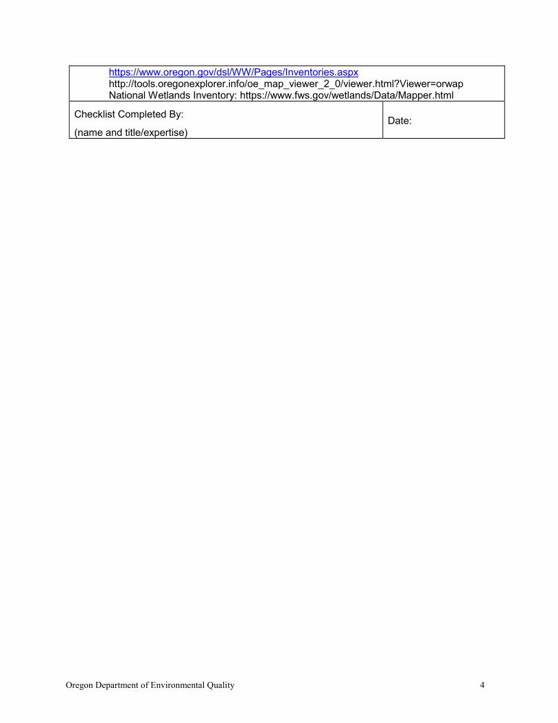
https://www.oregon.gov/dsl/WW/Pages/Inventories.aspx http://tools.oregonexplorer.info/oe_map_viewer_2_0/viewer.html?Viewer=orwap National Wetlands Inventory: https://www.fws.gov/wetlands/Data/Mapper.html

Checklist Completed By:

(name and title/expertise) Date:

https://www.oregon.gov/dsl/WW/Pages/Inventories.aspx


Appendix A2: Exposure Pathway Assessment


Exposure Pathway Assessment This assessment is a conservative qualitative determination of whether there is any reason to believe that a complete or potentially complete pathway between contaminants of interest and ecological receptors exists or may exist in the locality of the facility. Locality of facility is defined in rule, and means any point where a human or an ecological receptor contacts, or is reasonably likely to come into contact with, facility-related hazardous substances, considering: a) the chemical and physical characteristics of the hazardous substances; b) physical, meteorological, hydrogeological, and ecological characteristics that govern the tendency for hazardous substances to migrate through environmental media or to move and accumulate through food webs; c) any human activities and biological processes that govern the tendency for hazardous substances to move into and through environmental media or to move and accumulate through food webs; and d) the time required for contaminant migration to occur based on the factors described above. Note there are three attachments to this Exposure Pathway Assessment Appendix. Attachments 1 and 2 should be completed and submitted to DEQ along with a report or technical memorandum that generally follows the outline provided in Attachment 3. General exposure pathway assessment tasks are described below and refer to relevant attachments.

Tasks (1) Assess existing data

Obtain the following information regarding the site and surrounding area for submittal to DEQ: (a) Surface area of the site; (b) Present and historical uses of the site and nearby properties; (c) Current and reasonably likely future land and/or water use(s); (d) Sensitive environments (as defined by OAR 340-122-115(49)) at, adjacent to, or in

the locality of the site; (e) Known or suspected presence of threatened and/or endangered species or their

habitat in the locality of the facility (see text box below for resources to determine the presence of T&E species).

(f) Accurate site and regional maps showing structures, infrastructure, sampling locations, land use, wetlands, surface water bodies, sensitive environments, etc.;

(g) Types of hazardous substances reportedly released at the site; (h) Magnitude and extent of migration of any hazardous substances reportedly released

at the site.


(2) Perform initial site visit A visit to the site to directly assess ecological features, transport pathways, and conditions is typically required, except at very ecologically simple sites where aerial photographs and infrastructure maps suffice. The site itself, areas adjacent to the site, and areas in the locality of the site (as defined by OAR 340-122-115(34)) should all be visited. The size and complexity of the site will determine the time needed for this initial visit. While at the site, the following activities should be performed: (a) Look for any signs (e.g. visual, olfactory, etc.) of a chemical release; (b) Sketch the site topography, with special emphasis to surface water drainages and

other potential hazardous substance migration pathways; (c) Note any evident (e.g. visual, olfactory, etc.) signs of hazardous substance

migration within the site or offsite; (d) Look for signs of threatened and/or endangered species or their habitat within or

adjacent to the site; (e) As appropriate, note any evident signs (seeps, springs, cutbanks, etc.) for

groundwater discharge to the surface; (f) Note any natural or anthropogenic disturbances onsite; (g) Make a photographic record of the site, with emphasis on ecological features and

potential exposure pathways;

Sources to Determine the Presence of Threatened and Endangered Species Oregon: Consultation with the Oregon Biodiversity Information Center (ORBIC), provides information on state and federally listed rate, threatened and endangered species in Oregon that may occur at your Site. ORBIC is a part of the Institute for Natural Resources (INR) which is a cooperative enterprise of Oregon's public universities. Request and submit a data request for the occurrence of rare, threatened, and endangered species for your Site. Data requests can be submitted electronically: https://inr.oregonstate.edu/orbic. The Center provides site-specific species information within two miles of the given location. Additional information and specific state and federal species lists can be found using the following resources.

• Oregon Listed: Oregon Department of Fish and Wildlife https://www.dfw.state.or.us/wildlife/diversity/species/threatened_endangered_candidate_list.asp

• Federally Listed: o U.S. Fish and Wildlife Service Information for Planning and Consultation

https://ecos.fws.gov/ipac/ o National Marine Fisheries Service

https://www.fisheries.noaa.gov/national/endangered-species-conservation/esa-threatened-endangered-species

Note: Additional coordination with state or federal natural resource trustees and/or tribes may be needed to identify all relevant receptors of concern.

https://inr.oregonstate.edu/home

https://inr.oregonstate.edu/orbic

https://www.dfw.state.or.us/wildlife/diversity/species/threatened_endangered_candidate_list.asp

https://www.dfw.state.or.us/wildlife/diversity/species/threatened_endangered_candidate_list.asp

https://ecos.fws.gov/ipac/




(h) Complete the Ecological Scoping Checklist (Attachment 1). (3) Identify contaminants of interest (COIs)

Identification of contaminants of interest for ecological receptors may necessitate a separate identification process than that used for any human health evaluation, since a contaminant not generally considered a threat to human health may be a threat to biota. The list of COIs are those known or suspected to be present based on the remedial investigation, and are identified based on site-specific sources of contamination. The results of this evaluation are summarized by completing Attachment 1, Parts and .

(4) Evaluate receptor-pathway interactions

Make an estimate, based on the site-specific information gathered in the previous three tasks and professional judgment, as to whether complete or potentially complete exposure pathways exist between COIs in a specific environmental media and ecologically important receptors associated with that media (e.g., between hazardous substances in surface water and fish). The results of this evaluation are summarized by completing Attachment 2. (a) For the purpose of completing Attachment 2, complete or potentially complete

exposure pathways are those that have: a source and mechanism for hazardous substance release to the environment, an environmental transport medium for the hazardous substance, a point of receptor contact (exposure point) with the contaminated media, and an exposure route to the receptor at the exposure point. (i) For upland assessments, an exposure point is any area not covered by

buildings, roads, paved areas or other barriers that would prevent wildlife from feeding on plants, earthworms, insects or other food or on the soil. Exposure areas generally exclude continuously disturbed or heavily landscaped areas adjacent to active operations that discourage wildlife use. Note that the absence of trees and shrubs does not eliminate exposure, as some species prefer areas with little or no vegetation (e.g., streaked horned lark and killdeer birds).

(ii) For aquatic assessments, an exposure point is sediment, wetland soils, and surface water.

(b) For the purpose of completing Attachment 2, the following species present in the LOF should be considered: (i) Individual listed threatened and endangered species; (ii) Local populations of species, including those that are recreational and/or

commercial resources; (iii) Local populations of any species with a known or suspected susceptibility

to the hazardous substance(s); (iv) Local populations of vertebrate species; (v) Local populations of invertebrate species, such as those that:


Provide food resource for higher organisms; or Perform a critical ecological function (such as organic matter

decomposition) ; or Can be used as a surrogate measure of adverse effects for individuals or

populations of other species. (c) For the purpose of completing Attachment 2, “plants are those that form the habitat

for local populations of species as defined above or are themselves listed as threatened and endangered species.

(d) Because they are not members of natural communities, any of the following should not be considered species of interest for the purpose of completing Attachment 2: (i) Pest and opportunistic species that populate an area entirely because of

artificial or anthropogenic conditions; (ii) Domestic animals (e.g., pets and livestock); (iii) Plants or animals whose existence is maintained by continuous human

intervention (e.g., fish hatcheries, agricultural crops). (5) Submit Tier I deliverable

This deliverable is a brief memorandum (see Attachment 3, Site Ecology Scoping Report, for suggested format and contents) detailing the results of the data review, site visit, and evaluation of receptors and pathways in the locality of the facility (LOF). It should present information in sufficient depth to give risk managers confidence in determining whether receptors and exposure pathways are or are not likely to exist at the site. (a) Attachment 3, Items 1a through 1g are 1-2 paragraph summaries of site conditions,

making reference to Items 4a through 4f as appropriate. (b) Attachment 3, Item 2a is Part of Attachment 1. (c) Attachment 3, Item 2b includes, at a minimum, Part of Attachment 1, as well as

any other site-specific observations that the responsible party wishes to include. (d) Attachment 3, Item 2c includes, at a minimum, Part of Attachment 1, as well as

any other site-specific observations that the responsible party wishes to include. (e) Attachment 3, Item 2d discusses efforts to observe species and/or habitats,

particularly listed threatened or endangered species (or their habitat) at or adjacent to the site. Any such species or habitats should be noted on Part of Attachment 1.

(f) Attachment 3, Item 2e includes, at a minimum, Attachment 2, as well as any other site-specific observations that the responsible party wishes to include.

(g) Attachment 3, Item 3 describes recommendations made on the basis of specific criteria.


(6) Determine whether potentially complete exposure pathways exist Based on information presented in the deliverable, do potential ecological receptors and potentially complete exposure pathways exist at or in the locality of the site? Specific criteria are as follows: (a) If any of the “Y” or “U” boxes in Attachment 2 are checked, then a recommendation

to move to risk assessment should be made. In completing this Attachment, a lack of knowledge, presence of high uncertainty, or any “unknown” circumstances should be tabulated as a “U”. (i) Note that a “Y” answer for any section requires that all three questions

within that section be answered “Y” or “U”. (b) If all of the “No” boxes in Attachment 2 are checked, then complete exposure

pathways to ecological receptors is unlikely, and therefore risk to ecological receptors is improbable. A recommendation for no further ecological investigations should be made.


ATTACHMENT 1 Ecological Scoping Checklist

Site Name Date of Site Visit Site Location Site Visit Conducted by

Part

CONTAMINANTS OF INTEREST IN LOCALITY OF FACILITY† Types, Classes, Or Specific Hazardous Substances ‡

Known Or Suspected Upland Aquatic

‡ As defined by OAR 340-122-115(30) † As defined by OAR 340-122-115(34) Part

OBSERVED IMPACTS OBSERVED IN THE LOCALITY OF THE FACILITY Finding Onsite vegetation (None, Limited, Extensive) Vegetation in the locality of the site (None, Limited, Extensive) Onsite wildlife such as macroinvertebrates, reptiles, amphibians, birds, mammals, other (None, Limited, Extensive)

Wildlife such as macroinvertebrates, reptiles, amphibians, birds, mammals, other in the locality of the site (None, Limited, Extensive)

Other readily observable impacts (None, Discuss below) Discussion:


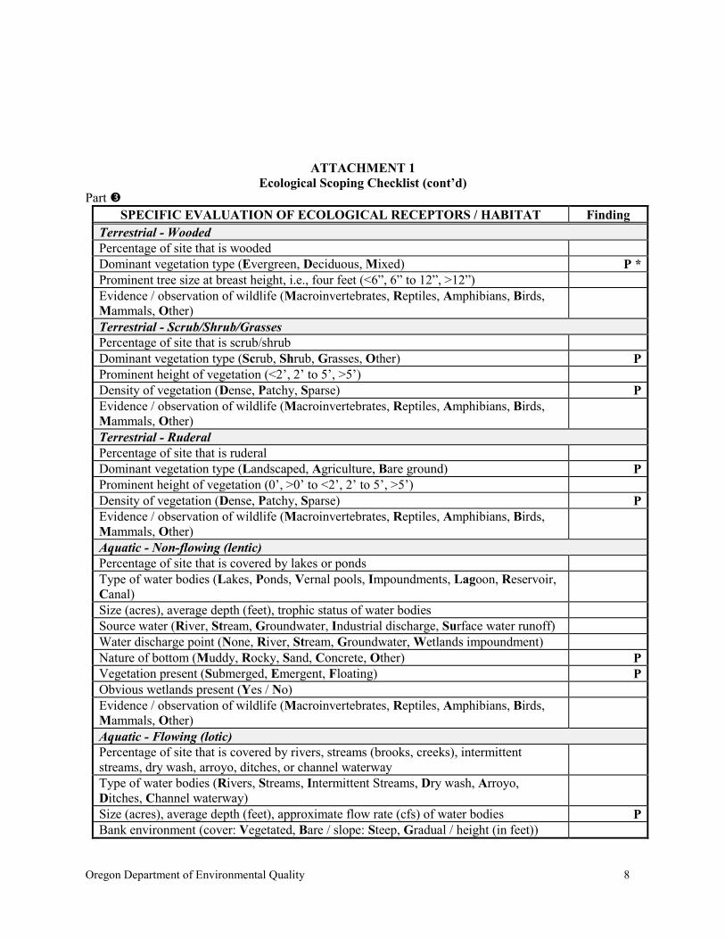
ATTACHMENT 1 Ecological Scoping Checklist (cont’d)

Part SPECIFIC EVALUATION OF ECOLOGICAL RECEPTORS / HABITAT Finding

Terrestrial - Wooded Percentage of site that is wooded Dominant vegetation type (Evergreen, Deciduous, Mixed) P * Prominent tree size at breast height, i.e., four feet (<6”, 6” to 12”, >12”) Evidence / observation of wildlife (Macroinvertebrates, Reptiles, Amphibians, Birds, Mammals, Other)

Terrestrial - Scrub/Shrub/Grasses Percentage of site that is scrub/shrub Dominant vegetation type (Scrub, Shrub, Grasses, Other) P Prominent height of vegetation (<2’, 2’ to 5’, >5’) Density of vegetation (Dense, Patchy, Sparse) P Evidence / observation of wildlife (Macroinvertebrates, Reptiles, Amphibians, Birds, Mammals, Other)

Terrestrial - Ruderal Percentage of site that is ruderal Dominant vegetation type (Landscaped, Agriculture, Bare ground) P Prominent height of vegetation (0’, >0’ to <2’, 2’ to 5’, >5’) Density of vegetation (Dense, Patchy, Sparse) P Evidence / observation of wildlife (Macroinvertebrates, Reptiles, Amphibians, Birds, Mammals, Other)

Aquatic - Non-flowing (lentic) Percentage of site that is covered by lakes or ponds Type of water bodies (Lakes, Ponds, Vernal pools, Impoundments, Lagoon, Reservoir, Canal)

Size (acres), average depth (feet), trophic status of water bodies Source water (River, Stream, Groundwater, Industrial discharge, Surface water runoff) Water discharge point (None, River, Stream, Groundwater, Wetlands impoundment) Nature of bottom (Muddy, Rocky, Sand, Concrete, Other) P Vegetation present (Submerged, Emergent, Floating) P Obvious wetlands present (Yes / No) Evidence / observation of wildlife (Macroinvertebrates, Reptiles, Amphibians, Birds, Mammals, Other)

Aquatic - Flowing (lotic) Percentage of site that is covered by rivers, streams (brooks, creeks), intermittent streams, dry wash, arroyo, ditches, or channel waterway

Type of water bodies (Rivers, Streams, Intermittent Streams, Dry wash, Arroyo, Ditches, Channel waterway)

Size (acres), average depth (feet), approximate flow rate (cfs) of water bodies P Bank environment (cover: Vegetated, Bare / slope: Steep, Gradual / height (in feet))


SPECIFIC EVALUATION OF ECOLOGICAL RECEPTORS / HABITAT Finding Source water (River, Stream, Groundwater, Industrial discharge, Surface water runoff) Tidal influence (Yes / No) Water discharge point (None, River, Stream, Groundwater, Wetlands impoundment) Nature of bottom (Muddy, Rocky, Sand, Concrete, Other) Vegetation present (Submerged, Emergent, Floating) Obvious wetlands present (Yes / No) Evidence / observation of wildlife (Macroinvertebrates, Reptiles, Amphibians, Birds, Mammals, Other)

Aquatic - Wetlands Obvious or designated wetlands present (Yes / No) Wetlands suspected as site is/has (Adjacent to water body, in Floodplain, Standing water, Dark wet soils, Mud cracks, Debris line, Water marks)

Vegetation present (Submerged, Emergent, Scrub/shrub, Wooded) Size (acres) and depth (feet) of suspected wetlands Source water (River, Stream, Groundwater, Industrial discharge, Surface water runoff) Water discharge point (None, River, Stream, Groundwater, Impoundment) Tidal influence (Yes / No) Evidence / observation of wildlife (Macroinvertebrates, Reptiles, Amphibians, Birds, Mammals, Other)

: Photographic documentation of these features is highly recommended. Part

HABITATS AND SPECIES OBSERVED OR DOCUMENTED IN LOF


ATTACHMENT 2 Evaluation of Receptor-Pathway Interactions

EVALUATION OF RECEPTOR-PATHWAY INTERACTIONS Y N U

Are hazardous substances present or potentially present in surface waters? This includes tidal or seasonally inundated areas and wetlands. AND Could hazardous substances reach these receptors via surface water?

When answering the above questions, consider the following: • Known or suspected presence of hazardous substances in surface waters. • Ability of hazardous substances to migrate to surface waters. Consider migration

pathways such as erosion of soils adjacent to aquatic environments (e.g., banks or riparian areas), subsurface preferential pathways (e.g., pipes), outfalls, groundwater discharges, and surface migration (e.g., ditches).

• Terrestrial organisms may be dermally exposed to water-borne contaminants as a result of wading or swimming in contaminated waters. Aquatic receptors may be exposed through osmotic exchange, respiration or ventilation of surface waters.

• Contaminants may be taken-up by terrestrial plants whose roots are in contact with surface waters.

• Terrestrial receptors may ingest water-borne contaminants if contaminated surface waters are used as a drinking water source.

Are hazardous substances present or potentially present in groundwater? AND Could hazardous substances reach these receptors via groundwater?

When answering the above questions, consider the following: • Known or suspected presence of hazardous substances in groundwater. • Ability of hazardous substances to migrate to groundwater. • Potential for hazardous substances to migrate via groundwater and discharge into

habitats and/or surface waters. • Contaminants may be taken-up by terrestrial and rooted aquatic plants whose roots are

in contact with groundwater present within the root zone (∼1m depth). • Terrestrial wildlife receptors generally will not contact groundwater unless it is

discharged to the surface.

“Y” = yes; “N” = No, “U” = Unknown (counts as a “Y”)


ATTACHMENT 2 Evaluation of Receptor-Pathway Interactions (cont’d)


Are hazardous substances present or potentially present in sediments? This includes tidal or seasonally inundated areas and wetlands. AND Could hazardous substances reach receptors via contact with sediments?

When answering the above questions, consider the following: • Known or suspected presence of hazardous substances in sediment. • Ability of hazardous substances to leach or erode from surface soils and be carried into

sediment via surface runoff. • Potential for contaminated groundwater to upwell through, and deposit contaminants in,

sediments. • If sediments are present in an area that is only periodically inundated with water, both

aquatic and terrestrial species may exposed. Aquatic receptors may be directly exposed to sediments or may be exposed through osmotic exchange, respiration or ventilation of sediment pore waters.

• Terrestrial species may be exposed to sediment in an area that is only periodically inundated with water.

• If sediments are present in an area that is only periodically inundated with water, terrestrial species may have direct access to sediments for the purposes of incidental ingestion. Aquatic receptors may regularly or incidentally ingest sediment while foraging.

Are hazardous substances present or potentially present in prey or food items of ecologically important receptors? AND Could hazardous substances reach these receptors via consumption of food items?

When answering the above questions, consider the following: • Higher trophic level terrestrial and aquatic consumers and predators may be exposed

through consumption of contaminated food sources. • In general, organic contaminants with log Kow > 3.5 may accumulate in terrestrial

mammals and those with a log Kow > 5 may accumulate in aquatic vertebrates.



ATTACHMENT 2 Evaluation of Receptor-Pathway Interactions (cont’d)


Are hazardous substances present or potentially present in surficial soils? AND Could hazardous substances reach these receptors via incidental ingestion of or dermal contact with surficial soils?

When answering the above questions, consider the following: • Known or suspected presence of hazardous substances in surficial (∼1m depth) soils. • Ability of hazardous substances to migrate to surficial soils. • Significant exposure via dermal contact would generally be limited to organic

contaminants which are lipophilic and can cross epidermal barriers. • Exposure of terrestrial plants to contaminants present in particulates deposited on leaf

and stem surfaces by rain striking contaminated soils (i.e., rain splash). • Contaminants in bulk soil may partition into soil solution, making them available to

roots. • Incidental ingestion of contaminated soil could occur while animals grub for food

resident in the soil, feed on plant matter covered with contaminated soil or while grooming themselves clean of soil.

Are hazardous substances present or potentially present in soils? AND Could hazardous substances reach these receptors via vapors or fugitive dust carried in surface air or confined in burrows?

When answering the above questions, consider the following: • Volatility of the hazardous substance (volatile chemicals generally have Henry’s Law

constant > 10-5 atm-m3/mol and molecular weight < 200 g/mol). • Exposure via inhalation is most important to organisms that burrow in contaminated

soils, given the limited amounts of air present to dilute vapors and an absence of air movement to disperse gases.

• Exposure via inhalation of fugitive dust is particularly applicable to ground-dwelling species that could be exposed to dust disturbed by their foraging or burrowing activities or by wind movement.

• Foliar uptake of organic vapors would be limited to those contaminants with relatively high vapor pressures.

• Exposure of terrestrial plants to contaminants present in particulates deposited on leaf and stem surfaces.



ATTACHMENT 3 Deliverable - Site Ecology Scoping Report

Outline (1) EXISTING DATA SUMMARY

(a) Site location (b) Site history (c) Site land and/or water use(s)

(i) Current (ii) Future

(d) Known or suspected hazardous substance releases (e) Sensitive environments (f) Threatened and/or endangered species (USFWS/ODFW/NMFS data)

(2) SITE VISIT SUMMARY

(a) Contaminants of Interest (Part , Attachment 1) (b) Observed impacts (Part , Attachment 1) (c) Ecological features (Part , Attachment 1) (d) Ecologically important species/habitats (Part , Attachment 1)

(i) Threatened and/or endangered species (ii) Threatened and/or endangered species habitat

(e) Exposure pathways (Attachment 2) (3) RECOMMENDATIONS (4) ATTACHMENTS

(a) Regional map showing location of site (b) Local map showing site in relation to adjacent property (c) Aerial photograph or map of LOF and adjacent areas within ¼ mile showing zoning,

current land use, location of surface water, critical habitat, and sensitive environments. (d) Topographic map (e) Figures showing source/release areas, estimated areas of contamination, and surface

features such as pavement, stormwater catch basins/drainage systems including outfalls, dry wells, or stormwater swales.

(f) Site photograph(s) (g) Documentation of the likelihood of T&E species to be present in the LOF.

(5) REFERENCES / DATA SOURCES


Appendix B: Upland Risk-Based Concentrations


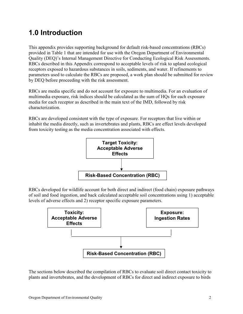
1.0 Introduction This appendix provides supporting background for default risk-based concentrations (RBCs) provided in Table 1 that are intended for use with the Oregon Department of Environmental Quality (DEQ)’s Internal Management Directive for Conducting Ecological Risk Assessments. RBCs described in this Appendix correspond to acceptable levels of risk to upland ecological receptors exposed to hazardous substances in soils, sediments, and water. If refinements to parameters used to calculate the RBCs are proposed, a work plan should be submitted for review by DEQ before proceeding with the risk assessment. RBCs are media specific and do not account for exposure to multimedia. For an evaluation of multimedia exposure, risk indices should be calculated as the sum of HQs for each exposure media for each receptor as described in the main text of the IMD, followed by risk characterization. RBCs are developed consistent with the type of exposure. For receptors that live within or inhabit the media directly, such as invertebrates and plants, RBCs are effect levels developed from toxicity testing as the media concentration associated with effects.

RBCs developed for wildlife account for both direct and indirect (food chain) exposure pathways of soil and food ingestion, and back calculated acceptable soil concentrations using 1) acceptable levels of adverse effects and 2) receptor specific exposure parameters. The sections below described the compilation of RBCs to evaluate soil direct contact toxicity to plants and invertebrates, and the development of RBCs for direct and indirect exposure to birds

Toxicity: Acceptable Adverse

Effects

Risk-Based Concentration (RBC)

Exposure: Ingestion Rates

Target Toxicity: Acceptable Adverse

Effects

Risk-Based Concentration (RBC)


and mammals to soil, water, and air. RBC development is based on exposure and toxicity information found primarily in the following national references:

1. EPA, 2005. Guidance for Developing Ecological Soil Screening Levels, OSWER 9285.7-55, Attachments and Contaminant Specific Ecological Soil Screening Level (Eco-SSL) documents (https://www.epa.gov/chemical-research/interim-ecological-soil-screening-level-documents)

2. LANL (Los Alamos National Laboratory), September 2017. “ECORISK Database (Release 4.1)”, LA-UR-17-26376, Los Alamos Laboratory, Los Alamos, New Mexico (https://www.intellusnm.com/). Go to the Documents section in the Intellus header bar, navigate to LANL Files >> Ecorisk Database, and download both .zip files in that directory ).

1.2 Terrestrial Plant and Invertebrates RBCs Plant and invertebrate soil RBCs are concentrations below which toxic effects are not expected on plant and invertebrate populations were taken from LANL, 2017. In this case, the RBC is equal to the toxicity reference value in units of mg/kg soil. A compilation of these RBCs are presented in Table 1.

1.3 Wildlife RBCs For each chemical and exposure media, the goal of the analysis was to develop RBCs representative of receptor guilds assessment endpoints for receptor functional groups, which are species that share similar feeding and physiological traits. The receptor groups are consistent include the following functional guilds:

• Mammalian Ground Feeding Herbivores and Omnivores: Mammal species that feed primarily on plants, or a mixed diet of plants and invertebrates.

• Mammalian Ground Feeding Insectivore: Mammal species that feed exclusively on invertebrates

• Mammalian Top Predators : Mammal species that feed 1) exclusively on small mammals and 2) primarily carnivores but diet may also invertebrates, and plants

• Avian Ground Feeding Herbivores and Omnivores: Bird species that feed primarily on plants, or a mixed diet of plants and invertebrates

• Avian Ground Feeding Insectivore: Bird species that feed exclusively on invertebrates • Avian Top Predators: Bird species that feed 1) exclusively on small mammals and 2)

primarily carnivores but diet may also invertebrates, and plants DEQ reviewed sources of national media risk based concentrations (RBCs) cited above consistent with goals outlined by DEQ’s default receptor guilds). RBCs are available for a range of functional groups and hazardous substances, including metals, organic chemicals including

https://www.intellusnm.com/


pesticides, polychlorinated biphenyls, and polychlorinated dibenzodioxins/furans for a range of exposure media including soil, water, air, and sediment.

2.0 Wildlife RBC Calculation RBC calculations require input on four variables related to exposure and toxicity of each feeding guild to calculate a media concentration representative of acceptable risk levels. The parameters include:

1. Toxicity Reference Values (TRV) 2. Food Intake Rates (FIR) 3. Proportion (or fraction) of total food intake that is soil 4. Transfer factors that estimate concentration in diet

The RBC calculations are outlined in EPA and LANL sources. The comparison of an acceptable risk concentration (considering NOAEL or LOAEL dose) with an environmental exposure concentration results in a hazard quotient (HQ). Equations from EPA soil RBCs are shown below, which uses the ratio of the exposure estimate to the TRV to calculate media concentrations representative of acceptable risk (HQ=1.0). If the exposure level is higher than the toxicity value, then there is the potential for risk to the receptor.

HQ= (Exposure Estimate)/TRV Exposure is estimated from calculated chemical intake of incidental soil ingestion and ingestion of biota as food:

Exposure Estimate= [(Cs×Ps×FIR) + (Cbiota×FIR)] Therefore:

HQ= [(Cs×Ps×FIR) + (Cbiota×Pb×FIR)]/TRV Where: Cs = concentration of contaminant in soil (mg/Kg [dry weight]) Ps = Soil ingestion as proportion of diet (unitless) Pb = Biota ingestion as proportion of diet (unitless) FIR = food ingestion rate (kg food [dry weight]/kg body weight [wet weight]/day) Cbiota = Concentration of contaminant in biota (mg/Kg [dry weight]) TRV = toxicity reference value The RBCs are calculated by solving the above general equation for the concentration in soil (Cs) that represents acceptable risk (HQ = 1.0). HQs that exceed 1.0 suggest that adverse effects are


possible. This calculation requires chemical- and receptor-specific values for the TRV, and knowledge about the relationship between soil (Cs) and uptake into biota (Cbiota). Similar equations are used to develop media concentrations for water and air as shown below and presented in LANL 2017. The following sections provide specific information on sources of TRVs (Section 3) and exposure parameters (Section 4) used in the analysis. Equations for the calculation of soil, water, and air RBCs are presented in LANL ECORISK database and shown below:

Water:


Additional RBCs are available that evaluate sediment borne-contamination to aerial birds and mammals exposed to emergent insects in LANL, 2017.

3.0 Toxicity Reference Values Toxicity reference values (TRVs) are chemical concentrations where adverse impacts attributable to chemical exposure are unlikely. In the case of wildlife, the acceptable dose of a chemical taken in by a receptor relative to body weight is used (mg chemical / kg body weight per day). For purposes of developing RBCs, TRVs are no observed effect concentrations (NOAELs) for threatened and endangered species, or the lowest observed effect concentrations (LOAELs) for all other species. TRVs are in units of dry weight (mg/kg bw/day) in order to facilitate the calculation of dry weight soil RBCs. Conversion from wet weight to dry weight and body weight and ingestion rate assumptions are provided in EPA 2005 and Toxicity Reference Value Development Methods for the Los Alamos National Laboratory (LANL, 2014) .

3.1 Sources of Toxicity Reference Values EPA Eco-SSL TRV development and Los Alamos TRV compilation, methodology, and data quality review were used as the primary sources of no effect (NOAEL) and low effect (LOAEL) toxicity reference values. In cases where TRVs apply to classes of chemicals, such as the total of DDT and metabolites, total PCBs, and total low and high molecular weight PAHs, EPA TRVs were selected. TRV selection generally included the following hierarchy of TRV sources (as outlined in LANL, 2017):

No and low observed effect levels or concentrations (NOAEL / NOAECs and LOAEL / LOAECs) are readily available in the scientific literature, and are regularly updated and reviewed by regulatory agencies nationally. Effect doses or concentrations that correspond to an adverse effect response of 10% (EC10 or ED10) are preferred over effect levels if enough toxicological data is available to support the development of a reasonable dose response curve. As new information becomes available, it is DEQ’s intent to approve use of toxicity reference values that may be more accurate in predicting toxicity based on the best available science.


1. Published National TRVs from EPA’s Eco-SSL TRV development and associated data quality review and methodology (EPA 2005, Attachment 2-2 through 2-5).

2. Calculated geometric mean TRVs where 3 or more data points are available from primary literature studies

3. TRVs identified from a critical study using an ecologically relevant maximum NOAEL / NOEC effect level that is lower than the lowest reported LOAEL / LOAC effect level. Where a NOAEL was not available, a factor of 0.1 applied to the LOAEL to estimate a NOAEL. Where a LOAEL was not available, a factor of 5 was applied to a NOAEL to estimate a LOAEL.

4. TRVs secondary data sources such as Oak Ridge National Laboratory (ORNL, 1996) The details of TRV development for each contaminant can be accessed through the LANL ECORISK database. A printable report is also available that from this database that summarizes the TRV development process.

4.0 Exposure Assumptions The default RBCs are calculated using reasonable maximum dietary composition for herbivores, omnivores, and carnivores. Food and soil ingestion rates for surrogates were representative of plausible upper-bound exposures, or reasonable maximum exposure (RME) (OAR 465.315(2)(B), to ensure protectiveness for other wildlife species within the same guild (EPA, 2015 Attachment 4-1), including:

1. Food Ingestion (kg-dry food/kg bw/day): High-end intake rates from EPA 2005

2. Soil Ingestion (Ps or fs): 90th percentile from the estimated distributions of proportion soil in diet (g absorbed per g dry mass) presented in EPA 2005 (Table 2, Appendix 4-1)

Exposure assumptions consistent with these objectives were taken from EPA Eco SSLs guidance, Attachment 4-1.EPA. LANL used similar exposure parameters for the ground feeding birds and mammals. Both sources selected surrogate species by considering body weight (a low body weight is associated with high food intake per unit body weight), and behavior (dietary sources, amount soil ingested). LANL differed from EPA in the selected exposure parameters for higher consumers such as carnivorous birds and mammals in order to be consistent with the physical and biological setting of north-central New Mexico (LANL 2012), and therefore may not represent reasonable maximum exposure for all Oregon species (e.g. weasels). Exposure parameters for the LANL surrogate receptor American Kestrel are also lower than guild specific parameters developed by EPA for the red-tailed hawk. Therefore, EPA exposure parameters for these species were used to calculate RBCs.


5.0 Uptake and Accumulation Estimation Equations representing uptake and accumulation relationships were taken from compilations presented in the EPA Eco-SSL guidance (EPA, 2005) and LANL ECORISK database represent the primary uptake factors used in RBC development.

6.0 Selected RBCs Table 1 presents NOAEL and LOAEL-based RBCs; Table 1a for terrestrial plants, invertebrates and wildlife exposed to soil, and Table 1b for surface water for terrestrial wildlife exposure, and NOAEL-based wildlife RBCs are intended for use when threatened and endangered species (T&E) are present. LOAEL-based RBCs are intended for use when no listed species are expected. This two-tier RBC system is intended to be used in screening risk assessments, and roughly corresponds to Oregon’s two levels of acceptable ecological risk [OAR 340-122-115(21)], where acceptable risk for T&E listed species is based on exposure of individual organisms that does not exceed the NOAEL based on reproductive effects. Acceptable risk for non-listed species is based on a probabilistic assessment that the probability is not greater than 10% (0.1) that 20 percent of the local population will experience exposures that exceed a median lethal dose or concentration (i.e., LD50 or LC50). In absence of a probabilistic risk assessment, the LOAEL-based RBC represents a higher level of risk for non-T&E species where the goal is to protect populations, not every individual. Chemical and physical properties govern the uptake into plants, invertebrates, and small mammals that comprise the dietary items of these different guilds. Therefore, the lowest RBCs calculated for herbivorous, omnivorous, insectivorous, and carnivorous exposure scenarios presented in Table 1a were selected represent RBCs protective of the four primary groups of birds and mammals (example surrogate receptors are shown in parenthesis). DEQ anticipates updating these values as new toxicity information becomes available.

1. Avian Ground Feeding Species (robin, woodcock, dove) 2. Mammalian Ground Feeding Species (shrew, vole, deer mouse, rabbit) 3. Higher Avian Consumers (kestrel, red-tailed hawk) 4. Higher Mammalian Consumers (fox, weasel)

RBCs for these groups are the lowest RBC for the following exposure scenarios: Avian Ground Feeding Species:

• LANL ESLs representing the robin herbivorous (100% plants), omnivorous (50% plants, 50% invertebrate), insectivorous (100% invertebrate) exposure scenarios


• EPA Eco-SSL representing the woodcock insectivorous and mourning dove granivorous (100% seeds) exposure scenarios

Mammalian Ground Feeding Species:

• LANL RBCs representing the montane shrew insectivorous (100% invertebrates), deer mouse omnivorous (50% plants, 50% invertebrate), and the cottontail herbivorous (100% plant) exposure scenarios

• EPA Eco-SSL representing the short-tailed shrew insectivorous (100% invertebrates) and meadow vole herbivorous (100% plant) exposure scenarios

Higher Avian Consumers:

• LANL Database TRVs and kestrel carnivorous (100% small mammal) and mixed diet (50% small mammal, 50% invertebrate) exposure scenarios

• EPA Eco-SSL TRVs and red-tailed hawk carnivorous (100% small mammal) exposure scenarios

• LANL TRVs and EPA carnivorous exposure scenarios for the red-tailed hawk (100% small mammal), DEQ calculated

Higher Mammalian Consumers:

• LANL Database TRVs and red fox carnivorous (100% small mammal) exposure scenario • EPA Eco-SSL TRVs and long-tailed weasel carnivorous (100% small mammal) exposure

scenario. • LANL TRVs and long-tailed weasel carnivorous (100% small mammal) exposure

scenarios, DEQ calculated

7.0 Site-Specific RBCs RBCs can be refined to reflect site-specific conditions or to evaluate additional species. Adjustments to default values, or data collection to determine site-specific transfer factors, should be done in coordination with DEQ. RBCs developed for additional species or contaminants of interest should be consistent with the exposure parameter and TRV methodology outlined in this Appendix, including ingestion rates representative of reasonable maximum exposure (RME) and TRV selection methods. The following technical details should be considered:

• Dose Conversions: Effects data are available in the literature as a dose in mg

contaminant/kg body weight/day, or as a concentration (mg contaminant/kg diet). NOAEL or LOAEL TRVs should be converted to units of mg contaminant/kg body weight/day using LANL, 2014. Body weight and wet-weight to dry-weight conversions used in TRV development should be presented

• Ingestion Rates: Ingestion rates for additional species should be developed in coordination with DEQ. Wet weight ingestion rates should be converted using the percent


moisture of the food used in the toxicity study used to develop the TRV and presented on a dry weight basis.

8.0 References Cited Baes, C.F., R. Sharp, A. Sjoreen and R. Shor. 1984. A Review and Analysis of Parameters for Assessing Transport of Environmentally Released Radionuclides through Agriculture. Prepared by Oak Ridge National Laboratory for U.S. Dept. of Energy. DEQ (Oregon Department of Environmental Quality). 2001. Guidance for Ecological Risk Assessment, Level II – Screening. EPA (US Environmental Protection Agency). 2005. Guidance for Developing Ecological Soil Screening Levels. OSWER Directive 9285.7-55. EPA (US Environmental Protection Agency). 2005. Attachment 4-1, Guidance for Developing Ecological Soil Screening Levels, Exposure Factors and Bioaccumulation Models for Derivation of Wildlife Eco-SSLs. OSWER Directive 9285.7-55. Jager, T. 1998. Mechanistic approach for estimating bioconcentration of organic chemicals in earthworms. Environ. Toxicol. Chem. 17: 2080-2090. Los Alamos National Laboratory, 2017. ECORISK Database User Guide, Revision 1. LA-UR-17-26376. Los Alamos National Laboratory, 2014. Toxicity Reference Value Development for the Los Alamos National Laboratory, Revision 1, LA-UR-20694. Ohio EPA (Ohio Environmental Protection Agency). 2008. Ecological Risk Assessment Guidance Document. Division of Environmental Response and Revitalization. Revised April 2008. Sample, B.W., D.M. Opresko, G.W. Sutter, II. 1996. Toxicological Benchmarks for Wildlife. Oak Ridge National Laboratory ES/ER/TM-86/R3. Lockheed Martin Energy Systems Environmental Restoration Program. Sample, B. E, J. J. Beauchamp, R. A. Efroymson, and G. W. Suter, II. 1998a. Development and Validation of Bioaccumulation Models for Small Mammals. Oak Ridge National Laboratory ES/ER/TM-219. Lockheed Martin Energy Systems Environmental Restoration Program. Sample, B. E, J. J. Beauchamp, R. A. Efroymson, G. W. Suter, II and T.L. Ashwood. 1998b. Development and Validation of Bioaccumulation Models for Earthworms. Oak Ridge National Laboratory ES/ER/TM-220. Lockheed Martin Energy Systems Environmental Restoration Program.


Ecological Risk Assessment IMD Attachment C: Risk-Based Concentrations for Water


The purpose of this appendix is to provide supporting background for risk-based concentrations (RBCs) provided in Table 2 that correspond to acceptable levels of ecotoxicological risk for hazardous substances in freshwater for benthic invertebrates, fish, amphibians, and plants exposed to surface water. Saltwater RBCs are not provided and will be developed on a site-specific basis with a similar approach and hierarchy to that used for freshwater criteria. The RBCs are intended for use with the Oregon Department of Environmental Quality (DEQ) guidance for ecological risk assessment. The compilation and hierarchy of RBCs, and any site-specific adjustments, are described below. Surface water RBCs are a compilation of criteria from a variety of sources, and account for chronic, including narcotic, effects and also effects to aquatic life and wildlife associated with accumulation in the food chain. All three categories of RBCs (i.e., chronic, narcotic, and consumption-based) should be considered for screening; however, note that not all RBC categories are relevant for every contaminant. The RBCs that are appropriate at each site will depend on the site-specific contaminants of interest. Additional details for each RBC category are provided below.

1. Chronic Criteria Aquatic life chronic criteria for toxic chemicals are the highest concentration of a specific pollutant that are not expected to pose a significant risk to the majority of a species in a given environment. These criteria incorporate testing with freshwater animals in eight different families including several families of fish, invertebrates, plants and typically an amphibian.

a. Contaminants of interest should be evaluated relative to the lower of the following:

i. Oregon State Aquatic Life Water Quality Criteria for Toxic Pollutants, Table 30; and

ii. National Recommended Water Quality Criteria – Aquatic Life Table 2 provides a summary of the criteria current as of this writing, and identifies the lower of the two as the chronic surface water RBC. It is important to note that some criteria are pH or hardness dependent, or in the case of copper require the use of a biotic ligand model to determine appropriate criteria. The values provided in Table 2 are calculated using an Oregon hardness default of 25 mg/L, however, site-specific adjustments may be made. It is important to review the information provided on the DEQ Water Quality Standards for Toxic Pollutants webpage https://www.oregon.gov/deq/wq/Pages/WQ-Standards-Toxics.aspx for the most current criteria development information and tools, such as a criteria calculator for hardness-dependent metals, an ammonia freshwater criteria calculator, more information on calculating the copper criteria using the biotic ligand model, and also recommendations for analysis for select contaminants.

b. For COIs for which no Oregon or National criteria are available, the Region 4

Surface Water Screening Values for Hazardous Waste Sites should be used. The most recent update of the Region 4 Ecological Risk Assessment Supplemental

https://www.oregon.gov/deq/wq/Pages/WQ-Standards-Toxics.aspx


Guidance should be used, and is currently found here: https://www.epa.gov/risk/regional-ecological-risk-assessment-era-supplemental-guidance. The March 2018 version current as of this writing provides criteria and supporting information in Tables 1a through 1c as follows:

Table 1a – Freshwater and Saltwater chronic and acute criteria Table 1b – Conversion Factors and Hardness-Dependent Equations Table 1c - Example Freshwater Screening Values for Varying Degrees of Water Hardness

Note that for screening values that are dependent on physical surface water conditions, such as hardness and pH, site-, region-, or Oregon-specific values should be used.

2. Narcotic Mode of Action Aquatic criteria associated with the narcotic mode of action should also be evaluated, to the extent chemicals associated with this mode of action are COIs at a site. The Region 4 Ecological Risk Assessment Supplemental Guidance provides these criteria. The March 2018 version (https://www.epa.gov/risk/regional-ecological-risk-assessment-era-supplemental-guidance), current as of this writing, provides criteria and supporting information in the following tables: Table 1d – Surface Water Screening Values for Narcotic Mode of Action Table 1e – Surface Water Screening Values for Polycyclic Aromatic Hydrocarbons

3. Bioaccumulative Chemicals If bioaccumulatives are contaminants of interest at a site, criteria protective of fish, birds, and mammals potentially exposed to contamination through consumption of food should be evaluated. The Region 4 Ecological Risk Assessment Supplemental Guidance provides these criteria. The March 2018 version (https://www.epa.gov/risk/regional-ecological-risk-assessment-era-supplemental-guidance), current as of this writing, provided the criteria in red font in Table 1a.

https://www.epa.gov/risk/regional-ecological-risk-assessment-era-supplemental-guidance







Ecological Risk Assessment IMD Attachment D: Tier III Probability of Exposure Ecological Risk Assessment


One option for a Tier III risk assessment is to determine the probability of exposure consistent with Oregon rule (OAR 340-122-0115(6)). Methodologies and examples are presented demonstrating how to conduct these assessments. Tier III requires more ecological information than a screening level risk assessment. Figure 1 summarizes the key pieces of information, and their relationships, needed to support a population risk characterization. Information about an assessment entity’s life history characteristics (e.g., home range, population density) and habitat preferences can be obtained from the literature. However, information about habitat conditions within and near the locality of the facility (LOF) can only be obtained by site visits and field surveys. Costs associated with obtaining and interpreting this additional information should be considered relative to the complexity of the site, and whether the analysis increase the relevancy of the risk assessment conclusions. This example of a Tier III ecological risk assessment provides two cases for how such information should be used in the evaluation of: 1) one habitat within the LOF and assessment population area (APA) and 2) multiple habitats within the LOF and assessment population area. The example shows how the binomial model is used in conjunction with habitat size and quality to determine if there is an acceptable population level risk. CASE 1 – ONE HABITAT AREA Site Characterization The legal boundaries of the site cover an area of 1 acre, but the dispersal of contamination (Chemical X in soil) has expanded the LOF to an area of 10.5 acres (Figure 2). The assessment entity is a small mammal, selected for its fidelity to the site, close contact with contaminated soil, and ecological role as prey for protected raptors. Because the small mammal has a small home range, its assessment population area is entirely within the LOF. A field survey reveals only one exposure area within the LOF (Figure 2) suitable for the small mammal. Exposure Assessment Because the habitat area and area of the LOF are approximately equal, the exposure point concentration is based on twenty samples collected within the LOF. Table 1 shows the chemical concentrations measured in soil. The data were found to be normally distributed. To use the binomial population risk model, variability in the Chemical X soil concentration must be propagated through to the dose estimate. In a simple case, this can be done by applying a deterministic exposure model to the soil concentration data. An exposure model converts a soil concentration into a dose of Chemical X to the small mammal from consumption of food items (soil invertebrates) that were themselves exposed to Chemical X in soil. The example exposure model is consistent with the model


used to develop default RBCs, and incorporates exposure from ingestion of soil, and soil invertebrates, as shown by the following equation. Dose = (IRsoil x Csoil x Sdry) + (IRfood x Cearthworm x Pdry x Pearthworm) Where: Dose = Exposure dose (mg/kg/day) Csoil = Concentration of Chemical X in soil (mg/kg dry weight) Sdry = Fraction of dry material in soil (0.80) IRsoil = Ingestion rate of soil (0.0063 kg/kg/day = 3% of IRfood) IRfood = Ingestion rate of food (0.209 kg/kg/day) Cearthworm = Concentration of Chemical X in earthworms (mg/kg dry weight) Pdry = Fraction of dry material in plants and earthworms (0.17) Pearthworm = Fraction of earthworms in diet (1.0) BW = Body weight of small mammal (0.015 kg) and:

Cearthworm = e[6.066 + (0.2372 x ln(Csoil))] The example equation for Cearthworm is typical of equations for calculating biota concentrations based on soil concentrations. These equations are chemical-specific, and can be obtained from sources such as Methods and Tools for Estimation of the Exposure of Terrestrial Wildlife to Contaminants (B.E. Sample, et al., Oak Ridge National Laboratory, ORNL/TM-13391, October 1997). In some cases it would be appropriate to include plants as a portion of the animal’s diet. In addition to regression relationships, EPA also uses partitioning relationships of worm to soil water (Kww), and water to soil (Kd) to calculate soil to earthworm bioaccumulation factors (BAFs) (USEPA, 2007). This approach can be applied where regression relationships are not available using chemical properties such as Kow. Based on EPA’s methodology, bioaccumulation factors (BAFs) can be calculated to estimate earthworm concentrations from soil concentrations. Biota concentrations calculated from dry weight concentrations in soil must be converted to wet weight concentrations before being used in an exposure assessment. In this example, Pdry is assumed to be 0.17, based an earthworm water content of 83%. Similarly, for direct soil ingestion, the dry weight soil concentration should be converted to a wet weight soil concentration before calculating the exposure dose. Soil moisture content is assumed to be 20%, so Sdry is assumed to be 0.80. Given the minor contribution to dose from soil ingestion, use of wet weight soil concentrations may not be important in most cases. The exposure doses shown in Table 1 were calculated by directly converting each soil concentration value to a dose. This approach allows for evaluation of the Case 1 example


data without the use of Monte Carlo methods. If a probabilistic approach is used, DEQ should be consulted regarding the choice of distributions. Effects Assessment A toxicity reference value (TRV), equivalent to an LD50, is selected from the literature. Although the TRV can be represented by a distribution, in most cases it will be a point estimate. In this example, the TRV for Chemical X is 46 mg/kg/day. Estimate Local Population Area Statute defines the acceptable risk level for protection of ecological receptors as the point before a significant adverse impact occurs to “a population of plants or animals in the locality of the facility”. ORS 465.315(1)(b)(A). Rule provides a quantitative definition of acceptable risk level for populations of ecological receptors that refers to the “total local population” OAR 340-122-0115(6). Local population is defined in the literature as:

• “A set of individuals that live in the same habitat patch and therefore interact with each other; most naturally applied to populations living in such small patches that all individuals share a comment environment” (Hanski and Simberloff, 1997).

• “The community of potentially interbreeding individuals at a given locality” (Mayr, 1970) which is partially based on “the relationship between mean mating probability of an individual within a given conspecific and distance”(e.g. dispersal distance) (Mayr,1970 and Wright, 1943).

• “A group of individuals within an investigator delineated area smaller then the geographic range of the species and often within a population.” (Wells and Richmond, 1995).

The literature cited in DEQ’s 1998 Guidance for Ecological Risk Assessment used dispersal distance, defined as the distance an animal moves from its natal home range, as a surrogate to estimate local population size (Waser, 1987). Waser et al., demonstrated that the probability of finding a mate within a few home ranges of its natal site is high-for both birds and mammals. In fact, if the probability is approximately 80% that a juvenile will find a mate within its natal home range (e.g., kangaroo rat and sparrows), then there is a 95 percent probability that a juvenile will find a mate within an area of 2 home ranges. If the probability is 40% that a juvenile will find a mate with its natal home range (e.g., deer mouse), there is a 95 percent probability a juvenile will find a mate within an area of 6 home ranges. This is supported by additional literature sources (Shields, 1982, Bowman et al., 2002). Based on this review, information on the home range together with considerations of the size of the locality of the facility (Wells and Richmond, 1995; ORS 465.315(1)(b)(A))


provide the key information needed to define the local population for ecological risk assessments. Information on home range is taken from the literature, such as U.S. EPA’s Wildlife Exposure Factors Handbook. If the home range of the receptor is larger than the locality of the facility (e.g. red tailed hawk, red fox) home range information along with population density data should be used to define the local assessment population. Area use factors may be used to adjust the exposure area. Alternatively, if the receptor’s home range is smaller or equal to the LOF, the LOF should be the starting point for defining local population assessment area. If the area of the LOF is equal to or less than approximately seven home ranges of the receptor of concern, use the LOF as the definition of the local population. Seven home ranges, supported by literature estimating probability related to dispersal distance (Waser, 1985, 1987), represent the original home range plus an area of six additional home ranges for potential dispersal (Bowman et al., 2002). If the LOF is larger than seven home ranges of the receptor of concern, multiple local population exposure areas should be developed within the LOF. In addition to dispersal information and area of the LOF, other factors related to landscape conditions that represent dispersal barriers should be considered in defining location population area. This may include roads, water bodies (streams, rivers, lakes). For the example provided in this appendix, the average home range of the receptor of concern is given as 0.5 acre. Estimate Local Population Abundance Information on population density can be taken from the literature, such as U.S. EPA’s Wildlife Exposure Factors Handbook, or scaling relationships can be used to calculate it. For this example, the annual average population density of the receptor is given as 6 individuals per acre. There would be, on average, 63 individuals within the 10.5 acre assessment population area (n = 63). Calculate p Given that the dose estimates appear to be normally distributed, and because the TRV is a point estimate, the following equation (a modified form of Equation 5 in DEQ’s Guidance for Ecological Risk Assessment) is used to estimate p, the probability that exposure to an individual small mammal will exceed the TRV.

−=

EXP

EXPZ s

TRVxp φ

where: p = Probability of exposure > TRV (unitless)


φZ = Cumulative distribution function of a standard normal random variable (MS-Excel® NORMSDIST function) xEXP = Mean of exposure dose (mg/kg/day) sEXP = Standard deviation of exposure dose (mg/kg/day) TRV = Point value of Toxicity Reference Value (mg/kg/day). Often, environmental data are found to be lognormally distributed instead of normally distributed. If the data had been lognormally distributed, the log transformation of both the dose and the TRV would be necessary. With a dose of 41 mg/kg/day, a standard deviation of 11 mg/kg/day, and a TRV of 46 mg/kg/day, p is calculated to be 0.36. In other words, there is a 36% chance that exposure (as dose) to an individual animal will exceed the TRV. Calculate b The definition of acceptable risk to an ecological population (OAR 340-122-0115(6)) requires an evaluation using the cumulative binomial function. The following equation is used to calculate b, the probability that more than 20% of the total local population will receive an exposure exceeding the TRV.

( ) ( )truepnyBINOMDISTppini

nb iniy

i,,,11

)!(!!1 )(

0−=

−

−

−= −

=∑

where: y = 20 percent of the population [y = INT(0.2n)] n = size of the local population (rounded down to a value evenly divisible by 5) p = probability of individual exposure > TRV b = probability that more than 20% of the total population will have exposure > TRV INT = MS-Excel® integer function BINOMDIST = MS-Excel® binomial distribution function (cumulative). The cumulative BINOMDIST function calculates the probability that at most y percent of the population will be exposed to a dose greater than the TRV. To calculate the probability that more than y percent of the population will be exposed to a dose greater than the TRV, the expression 1 – BINOMDIST is used. The value of n should be rounded down to the nearest number evenly divisible by 5. This will avoid unrealistically high calculated values of b as an artifact of the calculation method given that y must be an integer. In this example, we calculate 63 animals in the local population. We will round this down and use n = 60. Twenty percent of the population equals 12, so y = 12. With n = 60, y = 12, and p = 0.36, b is calculated to be over 0.99, as shown in Table 2. The chance of more than 20% of the total local population being exposed to a dose equivalent to the LD50 is therefore greater than 99%. This probability exceeds DEQ’s limit of 10%, which means that there is an unacceptable risk to the small mammal population at the site.


Alternative Method Using Look-Up Table As an alternative to calculating b, DEQ prepared Table 7 as a look-up table. Find the calculated number of animals at your site in the first column, and then compare the calculated probability p of individual exposure greater than the TRV with the limit shown in the second column. If p is less than or equal to the limit, the population risk is acceptable. If p is greater than the limit, the population risk is unacceptable. In Case 1, using a population n = 60, the limit of individual probability of harm from Table 8 is 0.145. The calculated value of p = 0.36 is above this limit, so DEQ would determine that the risk to the population is unacceptable. This simple screening step can also be used with area and habitat weighting (Case 2). CASE 2 – CONSIDERATION OF MULTIPLE HABITAT AREAS Site Characterization This case is identical in most respects to Case 1. Here, however, the field survey reveals two habitat types within the LOF (Figure 2). These habitat types have different soil concentrations of Chemical X and different area sizes. Information on the small mammal’s life history indicates that these two habitat types are both suitable, but to different degrees (i.e., differing habitat quality) for this receptor. We assume that the small mammals are able to move between all the habitat types. Exposure Assessment Twenty soil samples were collected within Habitat Type A, and fifteen samples were collected within the larger Habitat Type B, as shown in Table 3. Habitat Type A has the same concentration characteristics as in Case 1. Habitat Type B has an arithmetic mean dose of 30 mg/kg/day, with an arithmetic standard deviation of 4.8 mg/kg/day. Both data sets were found to be normally distributed. Given these data, and assuming that small mammals have access to all habitat types, and that exposure can only occur in suitable habitat, we considered four ways to calculate exposure. Three approaches involve calculating weighted means and weighted standard deviations. The following equations can be used if the resulting weighted data are normally distributed or can be transformed to a normal distribution. This will likely not be possible with weighting. In these cases, Monte Carlo modeling can be used determine the individual probability of exceeding the LD50.


Calculation of Weighted Mean and Weighted Standard Deviation Weighted Mean

�̅�𝑥𝑤𝑤 =∑ 𝑤𝑤𝑖𝑖𝑥𝑥𝑖𝑖𝑛𝑛𝑖𝑖=1∑ 𝑤𝑤𝑖𝑖𝑛𝑛𝑖𝑖=1

Weighted Standard Deviation

𝑆𝑆𝑆𝑆𝑤𝑤 = �∑ 𝑤𝑤𝑖𝑖𝑛𝑛𝑖𝑖=1 (𝑥𝑥𝑖𝑖 − �̅�𝑥𝑤𝑤)2𝑛𝑛 − 1𝑛𝑛 ∑ 𝑤𝑤𝑖𝑖

𝑛𝑛𝑖𝑖=1

Where: xi = dose associated with sample i wi = weight associated with sample i n = number of samples ̅xw = weighted mean dose SDw = weighted standard deviation of dose Approaches to Consider Multiple Habitats (1) Combined Habitat Areas. Combine samples from the two habitat types, excluding any samples taken outside of habitat. The combined 35 soil samples result in a calculated arithmetic mean dose of 36 mg/kg/day, with an arithmetic standard deviation of 10.4 mg/kg/day. The data are normally distributed. (2) Habitat Area-Weighting. Calculate a habitat area-weighted estimate of exposure (i.e., by assuming exposure is proportional to the areal extent of suitable habitat types). Table 4 shows the calculation of habitat area-weighted soil dose. The habitat area-weighted arithmetic mean dose is 34 mg/kg/day, with a weighted standard deviation of 9.7 mg/kg/day. The weighted mean dose is slightly lower here because the largest habitat area is also the least contaminated. (3) Habitat Quality-Weighting. Calculate a habitat quality-weighted estimate of exposure (i.e., by assuming exposure is proportional to the quality of suitable habitat types). Table 5 shows the calculation of habitat quality-weighted soil dose. The habitat quality-weighted arithmetic mean dose is 39 mg/kg/day, with a weighted standard deviation of 10.9. mg/kg/day. The weighted mean dose is slightly higher here because the more contaminated area has the higher habitat quality. (4) Habitat Area- and Quality-Weighting. Calculate a habitat area- and quality-weighted estimate of exposure (i.e., by assuming exposure is proportional to both the areal extent and attractiveness of each habitat type). Table 6 shows the calculation of habitat area- and quality-weighted doses. The habitat area- and quality-weighted arithmetic mean dose is 38 mg/kg/day, with an arithmetic standard deviation of 10.8 mg/kg/day. The mean dose is influenced by the more attractive habitat (type A) having the highest soil concentrations.


Table 7 shows a comparison of values using the different calculation methods. Effects Assessment As in Case 1, the TRV for Chemical X is a point estimate of 45 mg/kg/day. Estimate Assessment Population Area As described for Case 1, the local assessment population area for the small mammal is estimated as 10.5 acres. However, suitable habitat covers only 7.5 acres within this local assessment population area, making 7.5 acres the basis for population abundance estimates. Estimate Local Population Abundance Using the same population density described for Case 1 (6 animals per acre), but considering only 7.5 acres of suitable habitat, gives an estimated local population abundance of, on average, 45 individuals (n = 45). Twenty percent of the population is 9, so y = 9. Calculate p The calculation of individual probabilities p is shown in Table 7. Because most of the weighted data did not show a discernible distribution, Monte Carlo evaluations were needed. Depending on the assumptions guiding the calculation of exposure, calculated values of p range from a low of a 12% chance of exposure (as applied dose) exceeding the TRV, to a high of 25%. Calculate b Table 7 shows the calculation of b, the probability that more than 20% of the total local population will receive an exposure exceeding the TRV. With n = 45, y = 9, and various values for p, calculated values of b range from a low of 3.8% chance of adverse effects in more than 20% of the total local population, to a high of a 73% chance. The approximately 4% result is acceptable, but the other results, being greater than 10%, show an unacceptable risk to the small mammal population. The 23% risk estimate is both reflective of the high heterogeneity in the combined data set and the lack of consideration of any ecological (i.e., habitat) considerations. As shown in Table 7, when habitat area alone is considered, risk is acceptable; however, when quality is also considered, risk becomes unacceptable (53%). The assumption is that receptors are more likely to be attracted to a higher quality habitat area, which, in this instance, is also the most contaminated. This example shows that it may be important to consider both habitat area and habitat quality in the population risk assessment. Alternative Method Using a Look-Up Table to Determine Acceptability


As with Case 1, b does not need to be calculated. Instead, the individual probability p can be compared with the limit shown in Table 8 for the appropriate value of n. Using the table results in the same conclusion that would be reached using the cumulative binomial function evaluation.


REFERENCES Bowman et al., 2002. Dispersal distance of mammals is proportional to home range size. Ecology 83(7): 2049-2055. Hanski, I. and D. Simberloff. The metapopulation approach. In: Hanski, I. and Gilpin, M (eds), Metapopulation biology, ecology, genetics and evolution. Academic Press, pp. 5-26. Mayer, E. 1970. Populations, species and evolution. Harvard University Press. Shields, W.M. 1982. Philopatry, interbreeding, and the evolution of sex. State University of New York Press, Albany, New York, USA. USEPA, 2007. Exposure Factors and Bioaccumulation Models for Derivation of Wildlife Eco-SSLs. In: Guidance for Developing Ecological Soil Screening Levels (Eco SSLs), Attachment 4-1, OSWER Directive 9285.7-55, pp 3-1 to 3-6. Available at: http://www.epa.gov/ecotox/ecossl/pdf/ecossl_attachment_4-1.pdf. Waser, P.M. 1985. Does competition drive dispersal? Ecology 66(4): 1170-1175. Waser, P.M. 1987. A model predicting dispersal distance distributions. In: Mammalian dispersal patterns: the effects of social structure on population genetics. University of Chicago Press, Chicogo IL. Wells J.V. and M.E. Richmond. 1995. Populations, metapopulations and species populations: what are they and who should care? Wildlife Society Bulletin 23(3): 458-462. Wright, S. 1943. Isolation by distance. Genetics 28: 114-138.


TABLE 1 Case 1 (Habitat Type A)

Concentration of Chemical X in Soil, and Calculated Exposure Dose

Concentration of Chemical X in Soil (mg/kg dry weight)

Dose of Chemical X (mg/kg/day)

71 43 5 23

10.5 27 59 41 160 52 420 66 37 36 48 39 26 33 118 48 63 41 64 41 5 23 83 44 100 46 63 41 145 51 23.5 33 280 60 37 36

Mean 41 Standard Deviation 11

Distribution Normal

TABLE 2 Case 1 (Habitat Type A)

Calculation of Probability b

Parameter Value Mean Dose 41 mg/kg/day Standard Deviation of Dose 11 mg/kg/day Toxicity Reference Value (TRV) 46 mg/kg/day Individual Probability (p) 0.33 Number of small mammals (n) 60 20% of small mammal population (0.2 x n) 12 Probability b 0.98


TABLE 3 Case 2 (Two Habitat Types)

Concentration of Chemical X in Soil, and Calculated Exposure Doses

Habitat Type A Habitat Type B Concentration (mg/kg dry wt)

Dose (mg/kg/day)

Concentration (mg/kg dry wt)

Dose (mg/kg/day)

71 43 5 23 5 23 11 27

10.5 27 23 32 59 41 26 33 160 52 37 36 420 66 43 38 37 36 22 32 48 39 20 31 26 33 19 31 118 48 27 34 63 41 9.5 26 64 41 5 23 5 23 18 31 83 44 5 23 100 46 17 30 63 41 145 51 23.5 33 280 60 37 36

Habitat A Mean Dose 41 Habitat B Mean Dose 30 Standard Deviation 11 Standard Deviation 4.8

Distribution Normal Distribution Normal

Combined Habitat Mean Dose 36.3

Standard Deviation 10.5


TABLE 4 Case 2

Calculation of Area-Weighted Dose

Habitat

Habitat Area HA (acres)

Area Fraction

(HA ÷ Total HA)

Mean Dose

(mg/kg/d)

Area-Weighted Dose (mg/kg/d)

[Dose × Area Fraction]

A 2.5 0.33 41 14 B 5 0.67 30 20 Total = 7.5 Total = 34

TABLE 5 Case 2

Calculation of Quality-Weighted Dose

Habitat

Habitat Quality

(HQ) (unitless)

Quality Fraction

(HQ ÷ Total HQ)

Mean Dose

(mg/kg/d)

Quality-Weighted Dose (mg/kg/d) [Dose × Quality

Fraction] A 1 0.80 41 33 B 0.25 0.20 30 6 Total = 39

TABLE 6 Case 2

Calculation of Area- and Quality-Weighted Dose

Habitat

Habitat Area HA (ha)

Habitat Quality

HQ (unitless)

Habitat Area & Quality Factor

(HA × HQ)

Habitat Area&Quality

Fraction (HA × HQ) ÷ ∑(HA × HQ)

Weighted Mean Dose

(mg/kg/d)

Area&Quality-Weighted Dose [Dose × (HA × HQ) ÷ ∑(HA

× HQ)] A 2.5 1.00 2.5 0.67 41 27 B 5 0.25 1.25 0.33 30 10 Total = 3.75 Total = 37


TABLE 7

Case 2 Effect of Different Weighting Methods

Variable No Weighting of Combined Habitat Areas

Habitat Area Weighting

Habitat Quality Weighting

Both Habitat Area and Quality Weighting

Mean Dose (mg/kg/day) 36 34 39 38

Standard Deviation of Dose (mg/kg/day)

10.4 9.5 10.9 10.8

Individual Probability p 0.17 0.12 0.25 0.22

Probability b 0.43 0.038 0.73 0.53 Note: n = 45; 0.2 x n = 9


TABLE 8 Acceptable Probabilities in a Tier III Ecological Local Population Study

If you have the following number of animals (n) in your local

population areaa

The calculated individual probability (p) of an animal

receiving a dose greater than the TRVb, must be less than or equal to

the following c 0.10

<10 0.11 10 - 14 0.115 15 - 19 0.12 20 - 24 0.125 25 - 29 0.13 30 - 39 0.135 40 - 49 0.14 50 - 74 0.145 75 - 99 0.152

100 – 199 0.157 > 200 0.168

d 0.20 Notes:

a) Calculated from the local population area and the density of animals in the area. b) Calculated using the normal distribution function applied to the calculated dose

(mean and standard deviation) compared to the toxicity reference value (TRV). Analysis may include area and habitat weighting.

c) A calculated individual probability of 0.10 or less will always result in acceptable risk regardless of the number of animals in the local population area.

d) A calculated individual probability of 0.20 or greater will always result in unacceptable risk regardless of the number of animals in the local population area.


Figure 1. Summary of Relationships Between Key Information Required to Perform a Population-Level Risk Assessment.

Select assessment entities

Field survey LOF Prepare habitat map Measure habitat area

Get assessment entity life history characteristics

Estimate habitat quality for

assessment entity

Sample LOF (inside and outside

of habitat areas)

Exposure assessment EPC ~ Dose

Build life history - specific exposure

model

Effects assessment LD 50 ~ TRV

Risk characterization (binomial model)

Estimate local assessment

population area

Estimate local population abundance


Figure 2. Locality of the Facility, Local Assessment Population Area, and Habitat Area Relationships for Case 1.

Locality of the facility

SITE

HABITAT A

Local Assessment Population Area


Figure 3 Locality of the Facility, Local Assessment Population Area, and Habitat Area Relationships

for Case 2.

Locality of the facility

SITE

HABITAT B

HABITAT A

Local Assessment Population Area