Appendices: UIC Permit R9UIC-CA1-FY16-1 · UIC Permit R9UIC-CA1-FY16-1 . APPENDIX C – EPA Reporting Forms Form 7520-8: Quarterly Injection WellMonitoring Report Form 7520-18: Completion

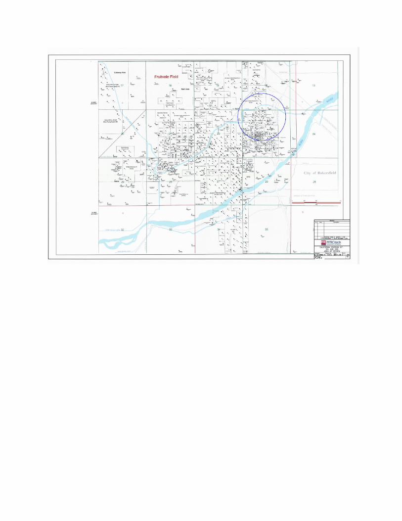
Appendix A

Project Location Maps

UIC Permit R9UIC-CA1-FY16-1

Appendix B

Well Schematics


Appendix C

EPA Reporting Forms


APPENDIX C – EPA Reporting Forms

Form 7520-8: Quarterly Injection Well Monitoring Report

Form 7520-18: Completion Report for Injection Wells

Form 7520-19: Well Rework Record, Plugging and Abandonment Plan, or Plugging and Abandonment Affidavit

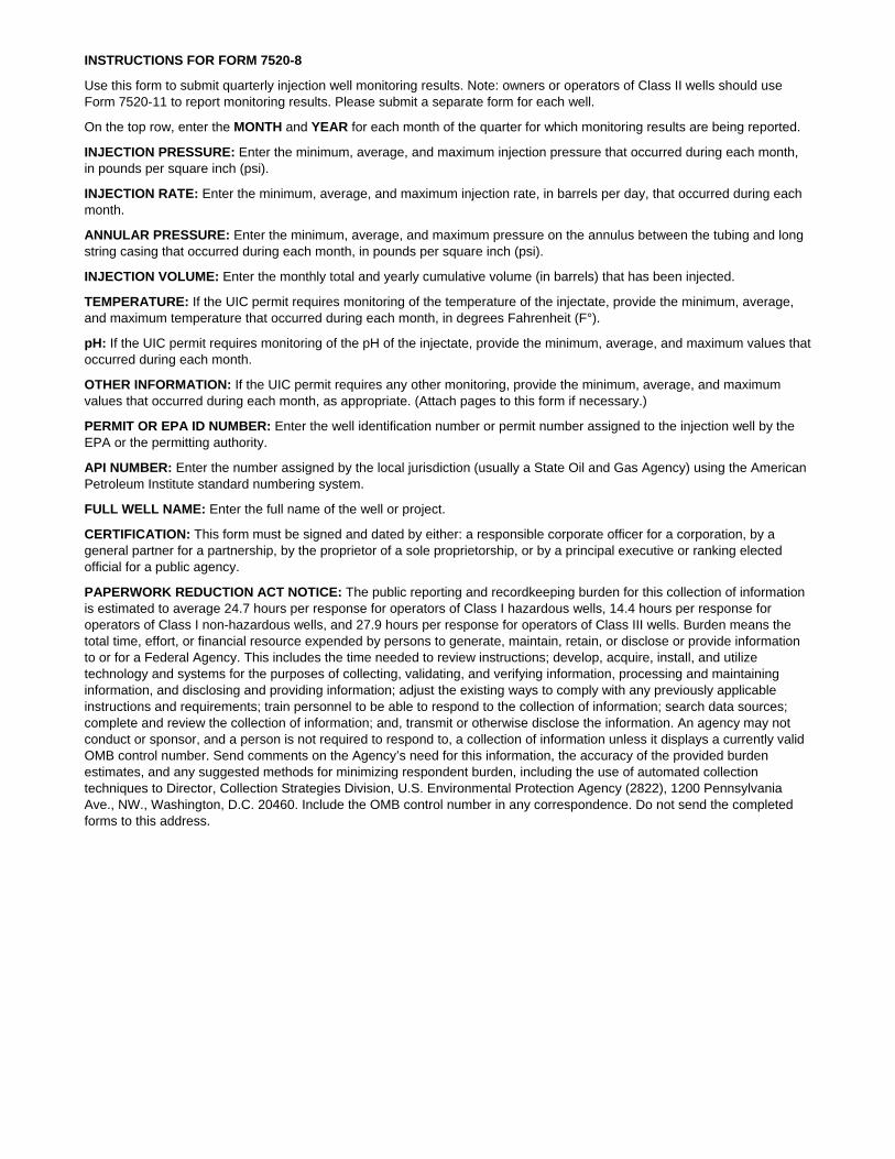
SEPA

OMB No. 2040-0042 Approval Expires 4/30/2022

United States Environmental Protection Agency

Quarterly Injection Well Monitoring Report

Month/Year Month/Year Month/Year

Injection Pressure (PSI)

1. Minimum

2. Average

3. Maximum

Injection Rate (Barrels/Day)

1. Minimum

2. Average

3. Maximum

Annular Pressure (PSI)

1. Minimum

2. Average

3. Maximum

Injection Volume (Barrels)

1. Monthly Total

2. Yearly Cumulative

Temperature (F °) - If Specified in UIC Permit

1. Minimum

2. Average

3. Maximum

pH - If Specified in UIC Permit

1. Minimum

2. Average

3. Maximum

Other Information Specified in the Permit (Attach Pages if Necessary)

Permit (or EPA ID) Number API Number Full Well Name

Certification I certify under the penalty of law that I have personally examined and am familiar with the information submitted in this document and all attachments and that, based on my inquiry of those individuals immediately responsible for obtaining the information, I believe that the information is true, accurate, and complete. I am aware that there are significant penalties for submitting false information, including the possibility of fine and imprisonmentt. (Ref. 40 CFR § 144.32)

Name and Official Title (Please type or print) Signature Date Signed

EPA Form 7520-8 (Rev. 4-19)

INSTRUCTIONS FOR FORM 7520-8

Use this form to submit quarterly injection well monitoring results. Note: owners or operators of Class II wells should use Form 7520-11 to report monitoring results. Please submit a separate form for each well.

On the top row, enter the MONTH and YEAR for each month of the quarter for which monitoring results are being reported.

INJECTION PRESSURE: Enter the minimum, average, and maximum injection pressure that occurred during each month, in pounds per square inch (psi).

INJECTION RATE: Enter the minimum, average, and maximum injection rate, in barrels per day, that occurred during each month.

ANNULAR PRESSURE: Enter the minimum, average, and maximum pressure on the annulus between the tubing and long string casing that occurred during each month, in pounds per square inch (psi).

INJECTION VOLUME: Enter the monthly total and yearly cumulative volume (in barrels) that has been injected.

TEMPERATURE: If the UIC permit requires monitoring of the temperature of the injectate, provide the minimum, average, and maximum temperature that occurred during each month, in degrees Fahrenheit (F°).

pH: If the UIC permit requires monitoring of the pH of the injectate, provide the minimum, average, and maximum values that occurred during each month.

OTHER INFORMATION: If the UIC permit requires any other monitoring, provide the minimum, average, and maximum values that occurred during each month, as appropriate. (Attach pages to this form if necessary.)

PERMIT OR EPA ID NUMBER: Enter the well identification number or permit number assigned to the injection well by the EPA or the permitting authority.

API NUMBER: Enter the number assigned by the local jurisdiction (usually a State Oil and Gas Agency) using the American Petroleum Institute standard numbering system.

FULL WELL NAME: Enter the full name of the well or project.

CERTIFICATION: This form must be signed and dated by either: a responsible corporate officer for a corporation, by a general partner for a partnership, by the proprietor of a sole proprietorship, or by a principal executive or ranking elected official for a public agency.

PAPERWORK REDUCTION ACT NOTICE: The public reporting and recordkeeping burden for this collection of information is estimated to average 24.7 hours per response for operators of Class I hazardous wells, 14.4 hours per response for operators of Class I non-hazardous wells, and 27.9 hours per response for operators of Class III wells. Burden means the total time, effort, or financial resource expended by persons to generate, maintain, retain, or disclose or provide information to or for a Federal Agency. This includes the time needed to review instructions; develop, acquire, install, and utilize technology and systems for the purposes of collecting, validating, and verifying information, processing and maintaining information, and disclosing and providing information; adjust the existing ways to comply with any previously applicable instructions and requirements; train personnel to be able to respond to the collection of information; search data sources; complete and review the collection of information; and, transmit or otherwise disclose the information. An agency may not conduct or sponsor, and a person is not required to respond to, a collection of information unless it displays a currently valid OMB control number. Send comments on the Agency’s need for this information, the accuracy of the provided burden estimates, and any suggested methods for minimizing respondent burden, including the use of automated collection techniques to Director, Collection Strategies Division, U.S. Environmental Protection Agency (2822), 1200 Pennsylvania Ave., NW., Washington, D.C. 20460. Include the OMB control number in any correspondence. Do not send the completed forms to this address.

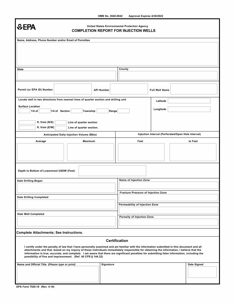
SEPA



COMPLETION REPORT FOR INJECTION WELLS

Name, Address, Phone Number and/or Email of Permittee

State County

Permit (or EPA ID) Number API Number Full Well Name

Locate well in two directions from nearest lines of quarter section and drilling unit

Surface Location

1/4 of 1/4 of Section Township Range

ft. from (N/S) Line of quarter section

ft. from (E/W) Line of quarter section.

Latitude

Longitude

Anticipated Daily Injection Volume (Bbls) Injection Interval (Perforated/Open Hole Interval)

Average Maximum Feet to Feet

Depth to Bottom of Lowermost USDW (Feet)

Date Drilling Began Name of Injection Zone

Fracture Pressure of Injection Zone

Date Drilling Completed

Permeability of Injection Zone

Date Well Completed Porosity of Injection Zone

Complete Attachments; See Instructions.

Certification I certify under the penalty of law that I have personally examined and am familiar with the information submitted in this document and all attachments and that, based on my inquiry of those individuals immediately responsible for obtaining the information, I believe that the information is true, accurate, and complete. I am aware that there are significant penalties for submitting false information, including the possibliity of fine and imprisonment. (Ref. 40 CFR § 144.32)


EPA Form 7520-18 (Rev. 4-19)

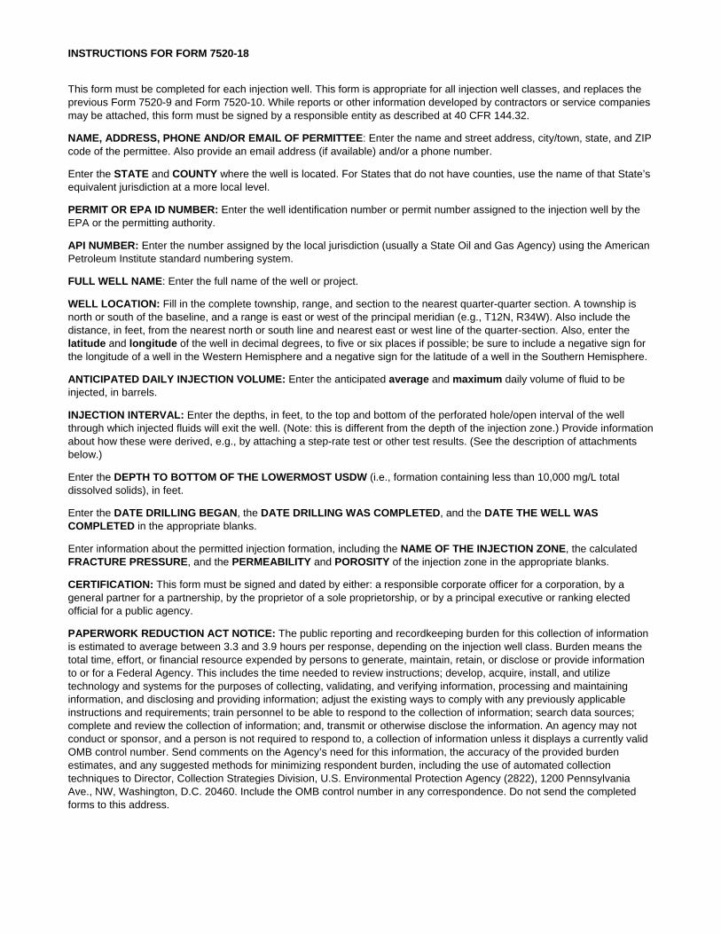
INSTRUCTIONS FOR FORM 7520-18

This form must be completed for each injection well. This form is appropriate for all injection well classes, and replaces the previous Form 7520-9 and Form 7520-10. While reports or other information developed by contractors or service companies may be attached, this form must be signed by a responsible entity as described at 40 CFR 144.32.

NAME, ADDRESS, PHONE AND/OR EMAIL OF PERMITTEE: Enter the name and street address, city/town, state, and ZIP code of the permittee. Also provide an email address (if available) and/or a phone number.

Enter the STATE and COUNTY where the well is located. For States that do not have counties, use the name of that State’s equivalent jurisdiction at a more local level.

PERMIT OR EPA ID NUMBER: Enter the well identification number or permit number assigned to the injection well by the EPA or the permitting authority.



WELL LOCATION: Fill in the complete township, range, and section to the nearest quarter-quarter section. A township is north or south of the baseline, and a range is east or west of the principal meridian (e.g., T12N, R34W). Also include the distance, in feet, from the nearest north or south line and nearest east or west line of the quarter-section. Also, enter the latitude and longitude of the well in decimal degrees, to five or six places if possible; be sure to include a negative sign for the longitude of a well in the Western Hemisphere and a negative sign for the latitude of a well in the Southern Hemisphere.

ANTICIPATED DAILY INJECTION VOLUME: Enter the anticipated average and maximum daily volume of fluid to be injected, in barrels.

INJECTION INTERVAL: Enter the depths, in feet, to the top and bottom of the perforated hole/open interval of the well through which injected fluids will exit the well. (Note: this is different from the depth of the injection zone.) Provide information about how these were derived, e.g., by attaching a step-rate test or other test results. (See the description of attachments below.)

Enter the DEPTH TO BOTTOM OF THE LOWERMOST USDW (i.e., formation containing less than 10,000 mg/L total dissolved solids), in feet.

Enter the DATE DRILLING BEGAN, the DATE DRILLING WAS COMPLETED, and the DATE THE WELL WAS COMPLETED in the appropriate blanks.

Enter information about the permitted injection formation, including the NAME OF THE INJECTION ZONE, the calculated FRACTURE PRESSURE, and the PERMEABILITY and POROSITY of the injection zone in the appropriate blanks.


PAPERWORK REDUCTION ACT NOTICE: The public reporting and recordkeeping burden for this collection of information is estimated to average between 3.3 and 3.9 hours per response, depending on the injection well class. Burden means the total time, effort, or financial resource expended by persons to generate, maintain, retain, or disclose or provide information to or for a Federal Agency. This includes the time needed to review instructions; develop, acquire, install, and utilize technology and systems for the purposes of collecting, validating, and verifying information, processing and maintaining information, and disclosing and providing information; adjust the existing ways to comply with any previously applicable instructions and requirements; train personnel to be able to respond to the collection of information; search data sources; complete and review the collection of information; and, transmit or otherwise disclose the information. An agency may not conduct or sponsor, and a person is not required to respond to, a collection of information unless it displays a currently valid OMB control number. Send comments on the Agency’s need for this information, the accuracy of the provided burden estimates, and any suggested methods for minimizing respondent burden, including the use of automated collection techniques to Director, Collection Strategies Division, U.S. Environmental Protection Agency (2822), 1200 Pennsylvania Ave., NW, Washington, D.C. 20460. Include the OMB control number in any correspondence. Do not send the completed forms to this address.

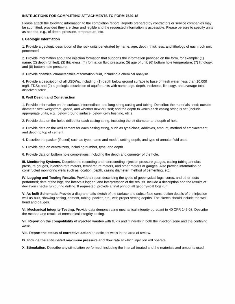
INSTRUCTIONS FOR COMPLETING ATTACHMENTS TO FORM 7520-18

Please attach the following information to the completion report. Reports prepared by contractors or service companies may be submitted, provided they are clear and legible and the requested information is accessible. Please be sure to specify units as needed, e.g., of depth, pressure, temperature, etc.

I. Geologic Information

1. Provide a geologic description of the rock units penetrated by name, age, depth, thickness, and lithology of each rock unit penetrated.

2. Provide information about the injection formation that supports the information provided on the form, for example: (1) name; (2) depth (drilled); (3) thickness; (4) formation fluid pressure; (5) age of unit; (6) bottom hole temperature; (7) lithology; and (8) bottom hole pressure.

3. Provide chemical characteristics of formation fluid, including a chemical analysis.

4. Provide a description of all USDWs, including: (1) depth below ground surface to base of fresh water (less than 10,000 mg/L TDS); and (2) a geologic description of aquifer units with name, age, depth, thickness, lithology, and average total dissolved solids.

II. Well Design and Construction

1. Provide information on the surface, intermediate, and long string casing and tubing. Describe: the materials used; outside diameter size; weight/foot, grade, and whether new or used; and the depth to which each casing string is set (include appropriate units, e.g., below ground surface, below Kelly bushing, etc.).

2. Provide data on the holes drilled for each casing string, including the bit diameter and depth of hole.

3. Provide data on the well cement for each casing string, such as type/class, additives, amount, method of emplacement, and depth to top of cement.

4. Describe the packer (if used) such as type, name and model, setting depth, and type of annular fluid used.

5. Provide data on centralizers, including number, type, and depth.

6. Provide data on bottom hole completions, including the depth and diameter of the hole.

III. Monitoring Systems. Describe the recording and nonrecording injection pressure gauges, casing-tubing annulus pressure gauges, injection rate meters, temperature meters, and other meters or gauges. Also provide information on constructed monitoring wells such as location, depth, casing diameter, method of cementing, etc.

IV. Logging and Testing Results. Provide a report describing the types of geophysical logs, cores, and other tests performed; date of the logs; the intervals logged; and interpretation of the results. Include a description and the results of deviation checks run during drilling. If requested, provide a final print of all geophysical logs run.

V. As-built Schematic. Provide a diagrammatic sketch of the surface and subsurface construction details of the injection well as-built, showing casing, cement, tubing, packer, etc., with proper setting depths. The sketch should include the well head and gauges.

VI. Mechanical Integrity Testing. Provide data demonstrating mechanical integrity pursuant to 40 CFR 146.08. Describe the method and results of mechanical integrity testing.

VII. Report on the compatibility of injected wastes with fluids and minerals in both the injection zone and the confining zone.

VIII. Report the status of corrective action on deficient wells in the area of review.

IX. Include the anticipated maximum pressure and flow rate at which injection will operate.

X. Stimulation. Describe any stimulation performed, including the interval treated and the materials and amounts used.

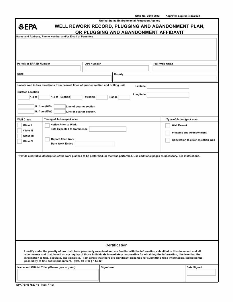
~EPA

I I I



WELL REWORK RECORD, PLUGGING AND ABANDONMENT PLAN, OR PLUGGING AND ABANDONMENT AFFIDAVIT

Name and Address, Phone Number and/or Email of Permittee

Permit or EPA ID Number API Number Full Well Name

State County

Locate well in two directions from nearest lines of quarter section and drilling unit Latitude

Surface Location Longitude

1/4 of 1/4 of Section Township Range

ft. from (N/S) Line of quarter section

ft. from (E/W) Line of quarter section.

Well Class Timing of Action (pick one) Type of Action (pick one)

Class I

Class II

Class III

Class V

Notice Prior to Work

Date Expected to Commence

Report After Work

Date Work Ended

Well Rework

Plugging and Abandonment

Conversion to a Non-Injection Well

Provide a narrative description of the work planned to be performed, or that was performed. Use additional pages as necessary. See instructions.

Certification I certify under the penalty of law that I have personally examined and am familiar with the information submitted in this document and all attachments and that, based on my inquiry of those individuals immediately responsible for obtaining the information, I believe that the information is true, accurate, and complete. I am aware that there are significant penalties for submitting false information, including the possibliity of fine and imprisonment. (Ref. 40 CFR § 144.32)


EPA Form 7520-19 (Rev. 4-19)

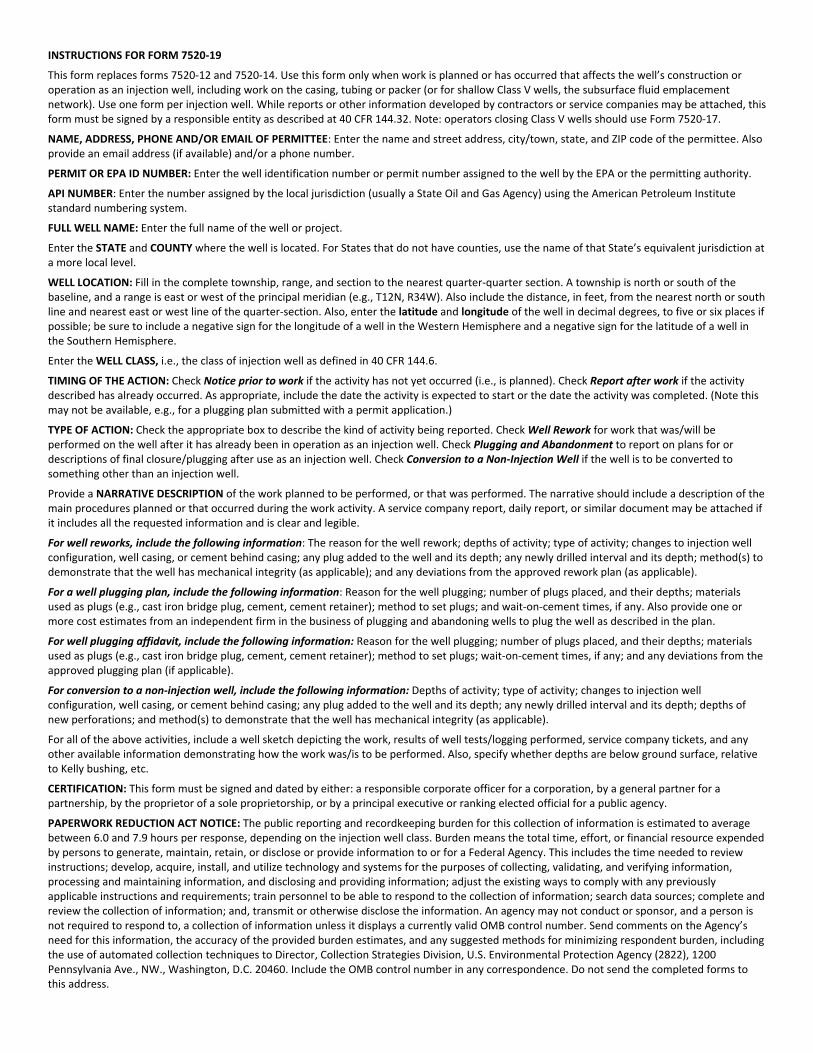
INSTRUCTIONS FOR FORM 7520‐19

This form replaces forms 7520‐12 and 7520‐14. Use this form only when work is planned or has occurred that affects the well’s construction or operation as an injection well, including work on the casing, tubing or packer (or for shallow Class V wells, the subsurface fluid emplacement network). Use one form per injection well. While reports or other information developed by contractors or service companies may be attached, this form must be signed by a responsible entity as described at 40 CFR 144.32. Note: operators closing Class V wells should use Form 7520‐17.

NAME, ADDRESS, PHONE AND/OR EMAIL OF PERMITTEE: Enter the name and street address, city/town, state, and ZIP code of the permittee. Also provide an email address (if available) and/or a phone number.

PERMIT OR EPA ID NUMBER: Enter the well identification number or permit number assigned to the well by the EPA or the permitting authority.



Enter the STATE and COUNTY where the well is located. For States that do not have counties, use the name of that State’s equivalent jurisdiction at a more local level.

WELL LOCATION: Fill in the complete township, range, and section to the nearest quarter‐quarter section. A township is north or south of the baseline, and a range is east or west of the principal meridian (e.g., T12N, R34W). Also include the distance, in feet, from the nearest north or south line and nearest east or west line of the quarter‐section. Also, enter the latitude and longitude of the well in decimal degrees, to five or six places if possible; be sure to include a negative sign for the longitude of a well in the Western Hemisphere and a negative sign for the latitude of a well in the Southern Hemisphere.

Enter the WELL CLASS, i.e., the class of injection well as defined in 40 CFR 144.6.

TIMING OF THE ACTION: Check Notice prior to work if the activity has not yet occurred (i.e., is planned). Check Report after work if the activity described has already occurred. As appropriate, include the date the activity is expected to start or the date the activity was completed. (Note this may not be available, e.g., for a plugging plan submitted with a permit application.)

TYPE OF ACTION: Check the appropriate box to describe the kind of activity being reported. Check Well Rework for work that was/will be performed on the well after it has already been in operation as an injection well. Check Plugging and Abandonment to report on plans for or descriptions of final closure/plugging after use as an injection well. Check Conversion to a Non‐Injection Well if the well is to be converted to something other than an injection well.

Provide a NARRATIVE DESCRIPTION of the work planned to be performed, or that was performed. The narrative should include a description of the main procedures planned or that occurred during the work activity. A service company report, daily report, or similar document may be attached if it includes all the requested information and is clear and legible.

For well reworks, include the following information: The reason for the well rework; depths of activity; type of activity; changes to injection well configuration, well casing, or cement behind casing; any plug added to the well and its depth; any newly drilled interval and its depth; method(s) to demonstrate that the well has mechanical integrity (as applicable); and any deviations from the approved rework plan (as applicable).

For a well plugging plan, include the following information: Reason for the well plugging; number of plugs placed, and their depths; materials used as plugs (e.g., cast iron bridge plug, cement, cement retainer); method to set plugs; and wait‐on‐cement times, if any. Also provide one or more cost estimates from an independent firm in the business of plugging and abandoning wells to plug the well as described in the plan.

For well plugging affidavit, include the following information: Reason for the well plugging; number of plugs placed, and their depths; materials used as plugs (e.g., cast iron bridge plug, cement, cement retainer); method to set plugs; wait‐on‐cement times, if any; and any deviations from the approved plugging plan (if applicable).

For conversion to a non‐injection well, include the following information: Depths of activity; type of activity; changes to injection well configuration, well casing, or cement behind casing; any plug added to the well and its depth; any newly drilled interval and its depth; depths of new perforations; and method(s) to demonstrate that the well has mechanical integrity (as applicable).

For all of the above activities, include a well sketch depicting the work, results of well tests/logging performed, service company tickets, and any other available information demonstrating how the work was/is to be performed. Also, specify whether depths are below ground surface, relative to Kelly bushing, etc.


PAPERWORK REDUCTION ACT NOTICE: The public reporting and recordkeeping burden for this collection of information is estimated to average between 6.0 and 7.9 hours per response, depending on the injection well class. Burden means the total time, effort, or financial resource expended by persons to generate, maintain, retain, or disclose or provide information to or for a Federal Agency. This includes the time needed to review instructions; develop, acquire, install, and utilize technology and systems for the purposes of collecting, validating, and verifying information, processing and maintaining information, and disclosing and providing information; adjust the existing ways to comply with any previously applicable instructions and requirements; train personnel to be able to respond to the collection of information; search data sources; complete and review the collection of information; and, transmit or otherwise disclose the information. An agency may not conduct or sponsor, and a person is not required to respond to, a collection of information unless it displays a currently valid OMB control number. Send comments on the Agency’s need for this information, the accuracy of the provided burden estimates, and any suggested methods for minimizing respondent burden, including the use of automated collection techniques to Director, Collection Strategies Division, U.S. Environmental Protection Agency (2822), 1200 Pennsylvania Ave., NW., Washington, D.C. 20460. Include the OMB control number in any correspondence. Do not send the completed forms to this address.

Appendix D

Logging Requirements


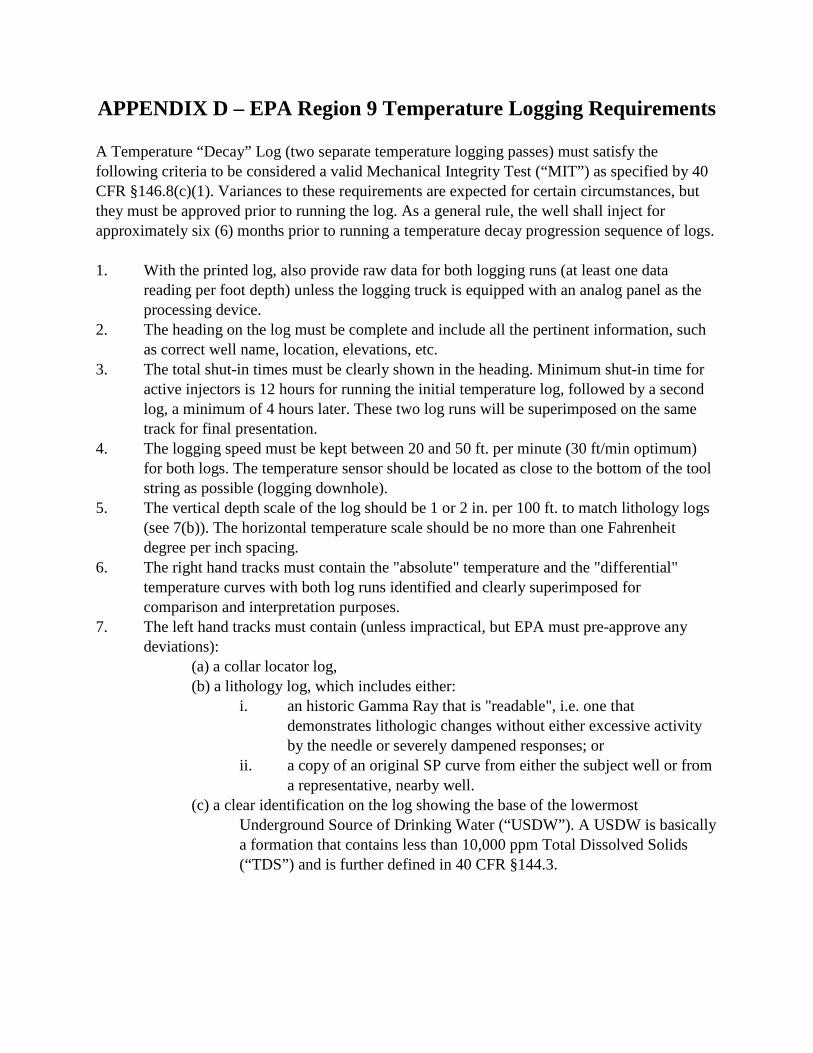
APPENDIX D – EPA Region 9 Temperature Logging Requirements

A Temperature “Decay” Log (two separate temperature logging passes) must satisfy the following criteria to be considered a valid Mechanical Integrity Test (“MIT”) as specified by 40 CFR §146.8(c)(1). Variances to these requirements are expected for certain circumstances, but they must be approved prior to running the log. As a general rule, the well shall inject for approximately six (6) months prior to running a temperature decay progression sequence of logs.

1. With the printed log, also provide raw data for both logging runs (at least one data reading per foot depth) unless the logging truck is equipped with an analog panel as the processing device.

2. The heading on the log must be complete and include all the pertinent information, such as correct well name, location, elevations, etc.

3. The total shut-in times must be clearly shown in the heading. Minimum shut-in time for active injectors is 12 hours for running the initial temperature log, followed by a second log, a minimum of 4 hours later. These two log runs will be superimposed on the same track for final presentation.

4. The logging speed must be kept between 20 and 50 ft. per minute (30 ft/min optimum) for both logs. The temperature sensor should be located as close to the bottom of the tool string as possible (logging downhole).

5. The vertical depth scale of the log should be 1 or 2 in. per 100 ft. to match lithology logs (see 7(b)). The horizontal temperature scale should be no more than one Fahrenheit degree per inch spacing.

6. The right hand tracks must contain the "absolute" temperature and the "differential" temperature curves with both log runs identified and clearly superimposed for comparison and interpretation purposes.

7. The left hand tracks must contain (unless impractical, but EPA must pre-approve any deviations):

(a) a collar locator log, (b) a lithology log, which includes either:

i. an historic Gamma Ray that is "readable", i.e. one that demonstrates lithologic changes without either excessive activity by the needle or severely dampened responses; or

ii. a copy of an original SP curve from either the subject well or from a representative, nearby well.

(c) a clear identification on the log showing the base of the lowermost Underground Source of Drinking Water (“USDW”). A USDW is basically a formation that contains less than 10,000 ppm Total Dissolved Solids (“TDS”) and is further defined in 40 CFR §144.3.

Appendix E

Region 9 UIC Pressure Falloff Requirements


EPA Region 9 UIC PRESSURE FALLOFF

REQUIREMENTS

Condensed version of the EPA Region 6

UIC PRESSURE FALLOFF TESTING GUIDELINE

Third Revision

• t, z w $i

August 8, 2002

TABLE OF CONTENTS

1.0 Background 2.0 Purpose of Guideline 3.0 Timing of Falloff Tests and Report Submission 4.0 Falloff Test Report Requirements 5.0 Planning

General Operational Concerns Site Specific Pretest Planning

6.0 Conducting the Falloff Test 7.0 Evaluation of the Falloff Test

1. Cartesian Plot 2. Log-log Plot 3. Semilog Plot 4. Anomalous Results

8.0 Technical References

APPENDIX Pressure Gauge Usage and Selection

Usage Selection

Test Design General Operational Considerations Wellbore and Reservoir Data Needed to Simulate or Analyze the Falloff Test Design Calculations Considerations for Offset Wells Completed in the Same Interval

Falloff Test Analysis Cartesian Plot Log-log Diagnostic Plot Identification of Test Flow Regimes Characteristics of Individual Test Flow Regimes

Wellbore Storage Radial Flow Spherical Flow Linear Flow Hydraulically Fractured Well Naturally Fractured Rock Layered Reservoir

Page 2 of 27

Semilog Plot Determination of the Appropriate Time Function for the Semilog Plot Parameter Calculations and Considerations Skin Radius of Investigation Effective Wellbore Radius Reservoir Injection Pressure Corrected for Skin Effects Determination of the Appropriate Fluid Viscosity Reservoir Thickness Use of Computer Software

Common Sense Check

Page 3 of 27

REQUIREMENTS

UIC PRESSURE FALLOFF TESTING GUIDELINE Third Revision August 8, 2002

1.0 Background

Region 9 has adopted the Region 6 UIC Pressure Falloff Testing Guideline requirements for monitoring Class 1 Non Hazardous waste disposal wells. Under 40 CFR 146.13(d)(1), operators are required annually to monitor the pressure buildup in the injection zone, including at a minimum, a shut down of the well for a time sufficient to conduct a valid observation of the pressure falloff curve.

All of the following parameters (Test, Period, Analysis) are critical for evaluation of technical adequacy of UIC permits: A falloff test is a pressure transient test that consists of shutting in an injection well and

measuring the pressure falloff. The falloff period is a replay of the injection preceding it; consequently, it is impacted by the magnitude, length, and rate fluctuations of the injection period. Falloff testing analysis provides transmissibility, skin factor, and well flowing and static pressures.

2.0 Purpose of Guideline

This guideline has been adopted by the Region 9 office of the Evironmental Protection Agency (EPA) to assist operators in planning and conducting the falloff test and preparing the annual monitoring report.

Falloff tests provide reservoir pressure data and characterize both the injection interval reservoir and the completion condition of the injection well. Both the reservoir parameters and pressure data are necessary for UIC permit demonstrations. Additionally, a valid falloff test is a monitoring requirement under 40 CFR Part 146 for all Class I injection wells.

The ultimate responsibility of conducting a valid falloff test is the task of the operator. Operators should QA/QC the pressure data and test results to confirm that the results “make sense” prior to submission of the report to the EPA for review.

Page 4 of 27

3.0 Timing of Falloff Tests and Report Submission

Falloff tests must be conducted annually. The time interval for each test should not be less than 9 months or greater than 15 months from the previous test. This will ensure that the tests will be performed at relatively even intervals.

The falloff testing report should be submitted no later than 60 days following the test. Failure to submit a falloff test report will be considered a violation and may result in an enforcement action. Any exceptions should be approved by EPA prior to conducting the test.

4.0 Falloff Test Report Requirements

In general, the report to EPA should provide: (1) general information and an overview of the falloff test, (2) an analysis of the pressure data obtained during the test, (3) a summary of the test results, and (4) a comparison of those results with previously used parameters.

Some of the following operator and well data will not change so once acquired, it can be copied and submitted with each annual report. The falloff test report should include the following information:

1. Company name and address 2. Test well name and location 3. The name and phone number of the facility contact person. The contractor contact may

be included if approved by the facility in addition to a facility contact person. 4. A photocopy of an openhole log (SP or Gamma Ray) through the injection interval

illustrating the type of formation and thickness of the injection interval. The entire log is not necessary.

5. Well schematic showing the current wellbore configuration and completion information: Χ Wellbore radius Χ Completed interval depths Χ Type of completion (perforated, screen and gravel packed, openhole)

6. Depth of fill depth and date tagged. 7. Offset well information:

Χ Distance between the test well and offset well(s) completed in the same interval or involved in an interference test

Χ Simple illustration of locations of the injection and offset wells 8. Chronological listing of daily testing activities. 9. Electronic submission of the raw data (time, pressure, and temperature) from all

pressure gauges utilized on CD-ROM. A READ.ME file or the disk label should list all files included and any necessary explanations of the data. A separate file containing any

Page 5 of 27

edited data used in the analysis can be submitted as an additional file. 10. Tabular summary of the injection rate or rates preceding the falloff test. At a

minimum, rate information for 48 hours prior to the falloff or for a time equal to twice the time of the falloff test is recommended. If the rates varied and the rate information is greater than 10 entries, the rate data should be submitted electronically as well as a hard copy of the rates for the report. Including a rate vs time plot is also a good way to illustrate the magnitude and number of rate changes prior to the falloff test.

11. Rate information from any offset wells completed in the same interval. At a minimum, the injection rate data for the 48 hours preceding the falloff test should be included in a tabular and electronic format. Adding a rate vs time plot is also helpful to illustrate the rate changes.

12. Hard copy of the time and pressure data analyzed in the report. 13. Pressure gauge information: (See Appendix, page A-1 for more information on

pressure gauges) Χ List all the gauges utilized to test the well Χ Depth of each gauge Χ Manufacturer and type of gauge. Include the full range of the gauge. Χ Resolution and accuracy of the gauge as a % of full range. Χ Calibration certificate and manufacturer's recommended frequency of calibration

14. General test information: Χ Date of the test Χ Time synchronization: A specific time and date should be synchronized to an

equivalent time in each pressure file submitted. Time synchronization should also be provided for the rate(s) of the test well and any offset wells.

Χ Location of the shut-in valve (e.g., note if at the wellhead or number of feet from the wellhead)

15. Reservoir parameters (determination): Χ Formation fluid viscosity, μf cp (direct measurement or correlation) Χ Porosity, φ fraction (well log correlation or core data) Χ Total compressibility, ct psi-1 (correlations, core measurement, or well test) Χ Formation volume factor, rvb/stb (correlations, usually assumed 1 for water) Χ Initial formation reservoir pressure - See Appendix, page A-1 Χ Date reservoir pressure was last stabilized (injection history) Χ Justified interval thickness, h ft - See Appendix, page A-15

16. Waste plume: Χ Cumulative injection volume into the completed interval Χ Calculated radial distance to the waste front, rwaste ft Χ Average historical waste fluid viscosity, if used in the analysis, μwaste cp

Page 6 of 27

17. Injection period: Χ Time of injection period Χ Type of test fluid Χ Type of pump used for the test (e.g., plant or pump truck) Χ Type of rate meter used Χ Final injection pressure and temperature

18. Falloff period: Χ Total shut-in time, expressed in real time and Δt, elapsed time Χ Final shut-in pressure and temperature Χ Time well went on vacuum, if applicable

19. Pressure gradient: Χ Gradient stops - for depth correction

20. Calculated test data: include all equations used and the parameter values assigned for each variable within the report Χ Radius of investigation, ri ft Χ Slope or slopes from the semilog plot Χ Transmissibility, kh/μ md-ft/cp Χ Permeability (range based on values of h) Χ Calculation of skin, s Χ Calculation of skin pressure drop, ΔPskin

Χ Discussion and justification of any reservoir or outer boundary models used to simulate the test

Χ Explanation for any pressure or temperature anomaly if observed 21. Graphs:

Χ Cartesian plot: pressure and temperature vs. time Χ Log-log diagnostic plot: pressure and semilog derivative curves. Radial flow

regime should be identified on the plot Χ Semilog and expanded semilog plots: radial flow regime indicated and the

semilog straight line drawn Χ Injection rate(s) vs time: test well and offset wells (not a circular or strip chart)

22. A copy of the latest radioactive tracer run and a brief discussion of the results.

5.0 Planning

The radial flow portion of the test is the basis for all pressure transient calculations. Therefore the injectivity and falloff portions of the test should be designed not only to reach radial flow, but to sustain a time frame sufficient for analysis of the radial flow period.

General Operational Concerns Χ Adequate storage for the waste should be ensured for the duration of the test

Page 7 of 27

Χ Offset wells completed in the same formation as the test well should be shut-in, or at a minimum, provisions should be made to maintain a constant injection rate prior to and during the test

Χ Install a crown valve on the well prior to starting the test so the well does not have to be shut-in to install a pressure gauge

Χ The location of the shut-in valve on the well should be at or near the wellhead to minimize the wellbore storage period

Χ The condition of the well, junk in the hole, wellbore fill or the degree of wellbore damage (as measured by skin) may impact the length of time the well must be shut-in for a valid falloff test. This is especially critical for wells completed in relatively low transmissibility reservoirs or wells that have large skin factors.

Χ Cleaning out the well and acidizing may reduce the wellbore storage period and therefore the shut-in time of the well

Χ Accurate recordkeeping of injection rates is critical including a mechanism to synchronize times reported for injection rate and pressure data. The elapsed time format usually reported for pressure data does not allow an easy synchronization with real time rate information. Time synchronization of the data is especially critical when the analysis includes the consideration of injection from more than one well.

Χ Any unorthodox testing procedure, or any testing of a well with known or anticipated problems, should be discussed with EPA staff prior to performing the test.

Χ If more than one well is completed into the same reservoir, operators are encouraged to send at least two pulses to the test well by way of rate changes in the offset well following the falloff test. These pulses will demonstrate communication between the wells and, if maintained for sufficient duration, they can be analyzed as an interference test to obtain interwell reservoir parameters.

Site Specific Pretest Planning

1. Determine the time needed to reach radial flow during the injectivity and falloff portions of the test: Χ Review previous welltests, if available Χ Simulate the test using measured or estimated reservoir and well completion

parameters Χ Calculate the time to the beginning of radial flow using the empirically-based

equations provided in the Appendix. The equations are different for the injectivity and falloff portions of the test with the skin factor influencing the falloff more than the injection period. (See Appendix, page A-4 for equations)

Χ Allow adequate time beyond the beginning of radial flow to observe radial flow so that a well developed semilog straight line occurs. A good rule of thumb is 3 to 5 times the time to reach radial flow to provide adequate radial flow data for analysis.

2. Adequate and consistent injection fluid should be available so that the injection rate into the test well can be held constant prior to the falloff. This rate should be high enough to

Page 8 of 27

produce a measurable falloff at the test well given the resolution of the pressure gauge selected. The viscosity of the fluid should be consistent. Any mobility issues (k/μ) should be identified and addressed in the analysis if necessary.

3. Bottomhole pressure measurements are required. (See Appendix, page A-2 for additional information concerning pressure gauge selection.)

4. Use two pressure gauges during the test with one gauge serving as a backup, or for verification in cases of questionable data quality. The two gauges do not need to be the same type. (See Appendix, page A-1 for additional information concerning pressure gauges.)

6.0 Conducting the Falloff Test

1. Tag and record the depth to any fill in the test well

2. Simplify the pressure transients in the reservoir Χ Maintain a constant injection rate in the test well prior to shut-in. This injection

rate should be high enough and maintained for a sufficient duration to produce a measurable pressure transient that will result in a valid falloff test.

Χ Offset wells should be shut-in prior to and during the test. If shut-in is not feasible, a constant injection rate should be recorded and maintained during the test and then accounted for in the analysis.

Χ Do not shut-in two wells simultaneously or change the rate in an offset well during the test.

3. The test well should be shut-in at the wellhead in order to minimize wellbore storage and afterflow. (See Appendix, page A-3 for additional information.)

4. Maintain accurate rate records for the test well and any offset wells completed in the same injection interval.

5. Measure and record the viscosity of the injectate periodically during the injectivity portion of the test to confirm the consistency of the test fluid.

7.0 Evaluation of the Falloff Test

1. Prepare a Cartesian plot of the pressure and temperature versus real time or elapsed time. Χ Confirm pressure stabilization prior to shut-in of the test well Χ Look for anomalous data, pressure drop at the end of the test, determine if

pressure drop is within the gauge resolution

2. Prepare a log-log diagnostic plot of the pressure and semilog derivative. Identify the Page 9 of 27

flow regimes present in the welltest. (See Appendix, page A-6 for additional information.) Χ Use the appropriate time function depending on the length of the injection period

and variation in the injection rate preceding the falloff (See Appendix, page A-10 for details on time functions.)

Χ Mark the various flow regimes - particularly the radial flow period Χ Include the derivative of other plots, if appropriate (e.g., square root of time for

linear flow) Χ If there is no radial flow period, attempt to type curve match the data

3. Prepare a semilog plot. Χ Use the appropriate time function depending on the length of injection period and

injection rate preceding the falloff Χ Draw the semilog straight line through the radial flow portion of the plot and

obtain the slope of the line Χ Calculate the transmissibility, kh/μ Χ Calculate the skin factor, s, and skin pressure drop, ΔP skin

Χ Calculate the radius of investigation, ri

4. Explain any anomalous results.

8.0 Technical References

1. SPE Textbook Series No. 1, “Well Testing,” 1982, W. John Lee 2. SPE Monograph 5, “Advances in Well Test Analysis,” 1977, Robert Earlougher, Jr. 3. SPE Monograph 1, “Pressure Buildup and Flow Tests in Wells,” 1967, C.S. Matthews

and D.G. Russell 4. “Well Test Interpretation In Bounded Reservoirs,” Hart’s Petroleum Engineer

International, Spivey, and Lee, November 1997 5. “Derivative of Pressure: Application to Bounded Reservoir Interpretation,” SPE Paper

15861, Proano, Lilley, 1986 6. “Well Test Analysis,” Sabet, 1991 7. “Pressure Transient Analysis,” Stanislav and Kabir, 1990 8. “Well Testing: Interpretation Methods,” Bourdarot, 1996 9. “A New Method To Account For Producing Time Effects When Drawdown Type Curves

Are Used To Analyze Pressure Buildup And Other Test Data,” SPE Paper 9289, Agarwal, 1980

10. “Modern Well Test Analysis – A Computer-Aided Approach,” Roland N. Horne, 1990 11. Exxon Monograph, “Well Testing in Heterogeneous Formations,” Tatiana Streltsova,

1987 12. EPA Region 6 Falloff Guidelines 13. “Practical Pressure Gauge Specification Considerations In Practical Well Testing,” SPE

Paper No. 22752, Veneruso, Ehlig-Economides, and Petitjean, 1991

Page 10 of 27

14. “Guidelines Simplify Well Test Interpretation,” Oil and Gas Journal, Ehlig-Economides, Hegeman, and Vik, July 18, 1994

15. Oryx Energy Company, Practical Pressure Transient Testing, G. Lichtenberger and K. Johnson, April 1990 (Internal document)

16. Pressure-Transient Test Design in Tight Gas Formations, SPE Paper 17088, W.J. Lee, October 1987

17. “Radius-of-Drainage and Stabilization-Time Equations,” Oil and Gas Journal, H.K. Van Poollen, Sept 14, 1964

18. “Effects of Permeability Anisotropy and Layering On Well Test Interpretation,” Hart’s Petroleum Engineer International, Spivey, Aly, and Lee, February 1998

19. “Three Key Elements Necessary for Successful Testing,” Oil and Gas Journal, Ehlig-Economides, Hegeman, Clark, July 25, 1994

20. “Introduction to Applied Well Test Interpretation,” Hart’s Petroleum Engineer International, Spivey, and Lee, August 1997

21. “Recent Developments In Well Test Analysis,” Hart’s Petroleum Engineer International, Stewart, August 1997

22. “Fundamentals of Type Curve Analysis,” Hart’s Petroleum Engineer International, Spivey, and Lee, September 1997

23. “Identifying Flow Regimes In Pressure Transient Tests,” Hart’s Petroleum Engineer International, Spivey and Lee, October 1997

24. “Selecting a Reservoir Model For Well Test Interpretation,” Hart’s Petroleum Engineer International, Spivey, Ayers, Pursell,and Lee, December 1997

27. “Use of Pressure Derivative in Well-Test Interpretation,” SPE Paper 12777, SPE Formation Evaluation Journal, Bourdet, Ayoub, and Pirard, June 1989

28. “A New Set of Type Curves Simplifies Well Test Analysis,” World Oil, Bourdet, Whittle, Douglas, and Pirard, May 1983

Page 11 of 27

APPENDIX Pressure Gauge Usage and Selection

Usage Χ EPA recommends that two gauges be used during the test with one gauge serving as a

backup. Χ Downhole pressure measurements are less noisy and are required. Χ A bottomhole surface readout gauge (SRO) allows tracking of pressures in real time.

Analysis of this data can be performed in the field to confirm that the well has reached radial flow prior to ending the test.

Χ The derivative function plotted on the log-log plot amplifies noise in the data, so the use of a good pressure recording device is critical for application of this curve.

Χ Mechanical gauges should be calibrated before and after each test using a dead weight tester.

Χ Electronic gauges should also be calibrated according to the manufacturer’s recommendations. The manufacturer's recommended frequency of calibration, and a copy of the gauge calibration certificate should be provided with the falloff testing report demonstrating this practice has been followed.

Selection Χ The pressures must remain within the range of the pressure gauge. The larger percent of

the gauge range utilized in the test, the better. Typical pressure gauge limits are 2000, 5000, and 10000 psi. Note that gauge accuracy and resolution are typically a function of percent of the full gauge range.

Χ Electronic downhole gauges generally offer much better resolution and sensitivity than a mechanical gauge but cost more. Additionally, the electronic gauge can generally run for a longer period of time, be programmed to measure pressure more frequently at various intervals for improved data density, and store data in digital form.

Χ Resolution of the pressure gauge must be sufficient to measure small pressure changes at the end of the test.

Test Design

General Operational Considerations Χ The injection period controls what is seen on the falloff since the falloff is replay of the

injection period. Therefore, the injection period must reach radial flow prior to shut-in of the well in order for the falloff test to reach radial flow

Χ Ideally to determine the optimal lengths of the injection and falloff periods, the test should be simulated using measured or estimated reservoir parameters. Alternatively, injection and falloff period lengths can be estimated from empirical equations using assumed reservoir and well parameters.

Page 12 of 27

Χ The injection rate dictates the pressure buildup at the injection well. The pressure buildup from injection must be sufficient so that the pressure change during radial flow, usually occurring toward the end of the test, is large enough to measure with the pressure gauge selected.

Χ Waste storage and other operational issues require preplanning and need to be addressed prior to the test date. If brine must be brought in for the injection portion of the test, operators should insure that the fluid injected has a consistent viscosity and that there is adequate fluid available to obtain a valid falloff test. The use of the wastestream as the injection fluid affords several distinct advantages: 1. Brine does not have to be purchased or stored prior to use. 2. Onsite waste storage tanks may be used. 3. Plant wastestreams are generally consistent, i.e., no viscosity variations

Χ Rate changes cause pressure transients in the reservoir. Constant rate injection in the test well and any offset wells completed in the same reservoir are critical to simplify the pressure transients in the reservoir. Any significant injection rate fluctuations at the test well or offsets must be recorded and accounted for in the analysis using superposition.

Χ Unless an injectivity test is to be conducted, shutting in the well for an extend period of time prior to conducting the falloff test reduces the pressure buildup in the reservoir and is not recommended.

Χ Prior to conducting a test, a crown valve should be installed on the wellhead to allow the pressure gauge to be installed and lowered into the well without any interruption of the injection rate.

Χ The wellbore schematic should be reviewed for possible obstructions located in the well that may prevent the use or affect the setting depth of a downhole pressure gauge. The fill depth in the well should also be reported. The fill depth may not only impact the depth of the gauge, but usually prolongs the wellbore storage period and depending on the type of fill, may limit the interval thickness by isolating some of the injection intervals. A wellbore cleanout or stimulation may be needed prior to conducting the test for the test to reach radial flow and obtain valid results.

Χ The location of the shut-in valve can impact the duration of the wellbore storage period. The shut-in valve should be located near the wellhead. Afterflow into the wellbore prolongs the wellbore storage period.

Χ The area geology should be reviewed prior to conducting the test to determine the thickness and type of formation being tested along with any geological features such as natural fractures, a fault, or a pinchout that should be anticipated to impact the test.

Wellbore and Reservoir Data Needed to Simulate or Analyze the Falloff Test Χ Wellbore radius, rw - from wellbore schematic

Page 13 of 27

⋅ ⋅

Χ Net thickness, h - See Appendix, page A-15 Χ Porosity, φ - log or core data Χ Viscosity of formation fluid, μf - direct measurement or correlations Χ Viscosity of waste, μwaste - direct measurement or correlations Χ Total system compressibility, ct - correlations, core measurement, or well test Χ Permeability, k - previous welltests or core data Χ Specific gravity of injection fluid, s.g. - direct measurement Χ Injection rate, q - direct measurement

Design Calculations When simulation software is unavailable the test periods can be estimated from empirical equations. The following are set of steps to calculate the time to reach radial flow from empirically-derived equations:

1. Estimate the wellbore storage coefficient, C (bbl/psi). There are two equations to calculate the wellbore storage coefficient depending on if the well remains fluid filled (positive surface pressure) or if the well goes on a vacuum (falling fluid level in the well): a. Well remains fluid filled:

C V c= ⋅w waste where, Vw is the total wellbore volume, bbls cwaste is the compressibility of the injectate, psi-1

b. Well goes on a vacuum: V uC = ρ⋅ g

144 ⋅ g c where, Vu is the wellbore volume per unit length, bbls/ft

ρ is the injectate density, psi/ft g and gc are gravitational constants

2. Calculate the time to reach radial flow for both the injection and falloff periods. Two different empirically-derived equations are used to calculate the time to reach radial flow, tradial flow, for the injectivity and falloff periods: a. Injectivity period:

200000 +12000s C⋅( )t > hoursradial flow k h⋅

μ b. Falloff period:

0.14⋅s170000 C et > hoursradial flow k h⋅ μ

The wellbore storage coefficient is assumed to be the same for both the injectivity and falloff periods. The skin factor, s, influences the falloff more than the injection period. Use these equations with caution, as they tend to fall apart for a well with a large

Page 14 of 27

permeability or a high skin factor. Also remember, the welltest should not only reach radial flow, but also sustain radial flow for a timeframe sufficient for analysis of the radial flow period. As a rule of thumb, a timeframe sufficient for analysis is 3 to 5 times the time needed to reach radial flow.

3. As an alternative to steps 1 and 2, to look a specific distance “L” into the reservoir and possibly confirm the absence or existence of a boundary, the following equation can be used to estimate the time to reach that distance:

948 ⋅φ ⋅ μ ⋅ c ⋅ Lt boundaryt = hoursboundary k where, Lboundary = feet to boundary

tboundary = time to boundary, hrs

Again, this is the time to reach a distance “L” in the reservoir. Additional test time is required to observe a fully developed boundary past the time needed to just reach the boundary. As a rule of thumb, to see a fully developed boundary on a log-log plot, allow at least 5 times the time to reach it. Additionally, for a boundary to show up on the falloff, it must first be encountered during the injection period.

4. Calculate the expected slope of the semilog plot during radial flow to see if gauge resolution will be adequate using the following equation:

162.6 ⋅ ⋅q Β m = semilog k h⋅ μ

where, q = the injection rate preceding the falloff test, bpd B = formation volume factor for water, rvb/stb (usually assumed to be 1)

Considerations for Offset Wells Completed in the Same Interval Rate fluctuations in offset wells create additional pressure transients in the reservoir and complicate the analysis. Always try to simplify the pressure transients in the reservoir. Do not simultaneously shut-in an offset well and the test well. The following items are key considerations in dealing with the impact of offset wells on a falloff test:

Χ Shut-in all offset wells prior to the test Χ If shutting in offset wells is not feasible, maintain a constant injection rate prior to and

during the test Χ Obtain accurate injection records of offset injection prior to and during the test Χ At least one of the real time points corresponding to an injection rate in an offset well

should be synchronized to a specific time relating to the test well Χ Following the falloff test in the test well, send at least two pulses from the offset well

to the test well by fluctuating the rate in the offset well. The pressure pulses can confirm communication between the wells and can be simulated in the analysis if observed at the test well. The pulses can also be analyzed as an interference test using an Ei type curve.

Page 15 of 27

Χ If time permits, conduct an interference test to allow evaluation of the reservoir without the wellbore effects observed during a falloff test.

Falloff Test Analysis

In performing a falloff test analysis, a series of plots and calculations should be prepared to QA/QC the test, identify flow regimes, and determine well completion and reservoir parameters. Individual plots, flow regime signatures, and calculations are discussed in the following sections.

Cartesian Plot Χ The pressure data prior to shut-in of the well should be reviewed on a Cartesian plot to

confirm pressure stabilization prior to the test. A well that has reached radial flow during the injectivity portion of the test should have a consistent injection pressure.

Χ A Cartesian plot of the pressure and temperature versus real time or elapsed time should be the first plot made from the falloff test data. Late time pressure data should be expanded to determine the pressure drop occurring during this portion of the test. The pressure changes should be compared to the pressure gauges used to confirm adequate gauge resolution existed throughout the test. If the gauge resolution limit was reached, this timeframe should be identified to determine if radial flow was reached prior to reaching the resolution of the pressure gauge. Pressure data obtained after reaching the resolution of the gauge should be treated as suspect and may need to be discounted in the analysis.

Χ Falloff tests conducted in highly transmissive reservoirs may be more sensitive to the temperature compensation mechanism of the gauge because the pressure buildup response evaluated is smaller. Region 6 has observed cases in which large temperature anomalies were not properly compensated for by the pressure gauge, resulting in erroneous pressure data and an incorrect analysis. For this reason, the Cartesian plot of the temperature data should be reviewed. Any temperature anomalies should be noted to determine if they correspond to pressure anomalies.

Χ Include the injection rate(s) of the test well 48 hours prior to shut-in on the Cartesian plot to illustrate the consistency of the injection rate prior to shut-in and to determine the appropriate time function to use on the log-log and semilog plots. (See Appendix, page A10 for time function selection)

Page 16 of 27

10000

1 ODO

a. 100 2 ai 0

10

~

,,,,,,,_ ..

~ 0.001

~

~ I

.... I

I

I 0.01

I oil!, ,... ' ,,,, \ ,.A"

r E .. ... I(

--

1111

0.1 10 Elapsed Time (hours) - Tp=24.0

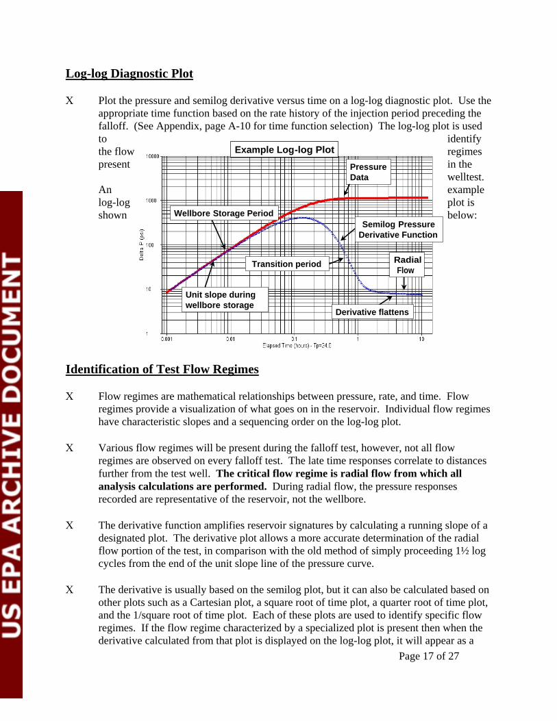
to identifythe flow Example Log-log Plot regimes present Pressure in the

Data welltest. An examplelog-log plot isshown Wellbore Storage Period below:

Transition period

Unit slope during wellbore storage

Radial Flow

Semilog Pressure Derivative Function

Derivative flattens

Log-log Diagnostic Plot

Χ Plot the pressure and semilog derivative versus time on a log-log diagnostic plot. Use the appropriate time function based on the rate history of the injection period preceding the falloff. (See Appendix, page A-10 for time function selection) The log-log plot is used

Identification of Test Flow Regimes

Χ Flow regimes are mathematical relationships between pressure, rate, and time. Flow regimes provide a visualization of what goes on in the reservoir. Individual flow regimes have characteristic slopes and a sequencing order on the log-log plot.

Χ Various flow regimes will be present during the falloff test, however, not all flow regimes are observed on every falloff test. The late time responses correlate to distances further from the test well. The critical flow regime is radial flow from which all analysis calculations are performed. During radial flow, the pressure responses recorded are representative of the reservoir, not the wellbore.

Χ The derivative function amplifies reservoir signatures by calculating a running slope of a designated plot. The derivative plot allows a more accurate determination of the radial flow portion of the test, in comparison with the old method of simply proceeding 1½ log cycles from the end of the unit slope line of the pressure curve.

Χ The derivative is usually based on the semilog plot, but it can also be calculated based on other plots such as a Cartesian plot, a square root of time plot, a quarter root of time plot, and the 1/square root of time plot. Each of these plots are used to identify specific flow regimes. If the flow regime characterized by a specialized plot is present then when the derivative calculated from that plot is displayed on the log-log plot, it will appear as a

Page 17 of 27

“flat spot” during the portion of the falloff corresponding to the flow regime.

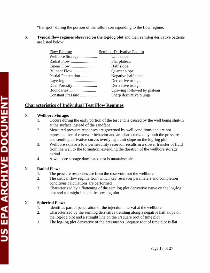
Χ Typical flow regimes observed on the log-log plot and their semilog derivative patterns are listed below:

Flow Regime Semilog Derivative Pattern Wellbore Storage ................. Unit slope Radial Flow ......................... Flat plateau Linear Flow ......................... Half slope Bilinear Flow ....................... Quarter slope Partial Penetration ............... Negative half slope Layering .............................. Derivative trough Dual Porosity ....................... Derivative trough Boundaries .......................... Upswing followed by plateau Constant Pressure ................ Sharp derivative plunge

Characteristics of Individual Test Flow Regimes

Χ Wellbore Storage: 1. Occurs during the early portion of the test and is caused by the well being shut-in

at the surface instead of the sandface 2. Measured pressure responses are governed by well conditions and are not

representative of reservoir behavior and are characterized by both the pressure and semilog derivative curves overlying a unit slope on the log-log plot

3. Wellbore skin or a low permeability reservoir results in a slower transfer of fluid from the well to the formation, extending the duration of the wellbore storage period

4. A wellbore storage dominated test is unanalyzable

Χ Radial Flow: 1. The pressure responses are from the reservoir, not the wellbore 2. The critical flow regime from which key reservoir parameters and completion

conditions calculations are performed 3. Characterized by a flattening of the semilog plot derivative curve on the log-log

plot and a straight line on the semilog plot

Χ Spherical Flow: 1. Identifies partial penetration of the injection interval at the wellbore 2. Characterized by the semilog derivative trending along a negative half slope on

the log-log plot and a straight line on the 1/square root of time plot 3. The log-log plot derivative of the pressure vs 1/square root of time plot is flat

Page 18 of 27

Χ Linear Flow: 1. May result from flow in a channel, parallel faults, or a highly conductive fracture 2. Characterized by a half slope on both the log-log plot pressure and semilog

derivative curves with the derivative curve approximately 1/3 of a log cycle lower than the pressure curve and a straight line on the square root of time plot. 3.

The log-log plot derivative of the pressure vs square root of time plot is flat

Χ Hydraulically Fractured Well: 1. Multiple flow regimes present including wellbore storage, fracture linear flow,

bilinear flow, pseudo-linear flow, formation linear flow, and pseudo-radial flow 2. Fracture linear flow is usually hidden by wellbore storage 3. Bilinear flow results from simultaneous linear flows in the fracture and from the

formation into the fracture, occurs in low conductivity fractures, and is characterized by a quarter slope on both the pressure and semilog derivative curves on the log-log plot and by a straight line on a pressure versus quarter root of time plot

4. Formation linear flow is identified by a half slope on both the pressure and semilog derivative curves on the log-log plot and by a straight line on a pressure versus square root of time plot

5. Psuedo-radial flow is analogous to radial flow in an unfractured well and is characterized by flattening of semilog derivative curve on the log-log plot and a straight line on a semilog pressure plot

Χ Naturally Fractured Rock: 1. The fracture system will be observed first on the falloff test followed by the total

system consisting of the fractures and matrix. 2. The falloff analysis is complex. The characteristics of the semilog derivative

trough on the log-log plot indicate the level of communication between the fractures and the matrix rock.

Χ Layered Reservoir: 1. Analysis of a layered system is complex because of the different flow regimes,

skin factors or boundaries that may be present in each layer. 2. The falloff test objective is to get a total tranmissibility from the whole reservoir

system. 3. Typically described as commingled (2 intervals with vertical separation) or

crossflow (2 intervals with hydraulic vertical communication)

Semilog Plot

Χ The semilog plot is a plot of the pressure versus the log of time. There are typically four different semilog plots used in pressure transient and falloff testing analysis. After plotting the appropriate semilog plot, a straight line should be drawn through the points located within the equivalent radial flow portion of the plot identified from the log-log

Page 19 of 27

plot.

Χ Each plot uses a different time function depending on the length and variation of the injection rate preceding the falloff. These plots can give different results for the same test, so it is important that the appropriate plot with the correct time function is used for the analysis. Determination of the appropriate time function is discussed below.

Χ The slope of the semilog straight line is then used to calculate the reservoir transmissibility - kh/μ, the completion condition of the well via the skin factor - s, and also the radius of investigation - ri of the test.

Determination of the Appropriate Time Function for the Semilog Plot The following four different semilog plots are used in pressure transient analysis: 1. Miller Dyes Hutchinson (MDH) Plot 2. Horner Plot 3. Agarwal Equivalent Time Plot 4. Superposition Time Plot These plots can give different results for the same test. Use of the appropriate plot with the correct time function is critical for the analysis.

Χ The MDH plot is a semilog plot of pressure versus Δt, where Δt is the elapsed shut-in time of the falloff. 1. The MDH plot only applies to wells that reach psuedo-steady state during

injection. Psuedo-steady state means the pressure response from the well has encountered all the boundaries around the well.

2. The MDH plot is only applicable to injection wells with a very long injection period at a constant rate. This plot is not recommended for use by EPA Region 6.

Χ The Horner plot is a semilog plot of pressure versus (tp+Δt)/Δt. The Horner plot is only used for a falloff preceded by a single constant rate injection period. 1. The injection time, tp=Vp/q in hours, where Vp=injection volume since the last

pressure equalization and q is the injection rate prior to shut-in for the falloff test. The injection volume is often taken as the cumulative injection since completion.

2. The Horner plot can result in significant analysis error if the injection rate varies prior to the falloff.

Χ The Agarwal equivalent time plot is a semilog plot of the pressure versus Agarwal equivalent time, Δte. 1. The Agarwal equivalent time function is similar to the Horner plot, but scales the

falloff to make it look like an injectivity test. 2. It is used when the injection period is a short, constant rate compared to the length

of the falloff period. 3. The Agarwal equivalent time is defined as: Δte=log(tp Δt)/(tp+Δt), where tp is

calculated the same as with the Horner plot. Page 20 of 27

Χ The superposition time function accounts for variable rate conditions preceding the falloff.

1. It is the most rigorous of all the time functions and is usually calculated using welltest software.

2. The use of the superposition time function requires the operator to accurately track the rate history. As a rule of thumb, at a minimum, the rate history for twice the length of the falloff test should be included in the analysis.

The determination of which time function is appropriate for the plotting the welltest on semilog and log-log plots depends on available rate information, injection period length, and software: 1. If there is not a rate history other than a single rate and cumulative injection, use a Horner

time function 2. If the injection period is shorter than the falloff test and only a single rate is available, use

the Agarwal equivalent time function 3. If you have a variable rate history use superposition when possible. As an alternative to

superposition, use Agarwal equivalent time on the log-log plot to identify radial flow. The semilog plot can be plotted in either Horner or Agarwal time if radial flow is observed on the log-log plot.

Parameter Calculations and Considerations

Χ Transmissibility - The slope of the semilog straight line, m, is used to determine the transmissibility (kh/μ) parameter group from the following equation:

k h⋅ 162.6 ⋅ ⋅q Β =

μ m

where, q = injection rate, bpd (negative for injection) B = formation volume factor, rvb/stb (Assumed to be 1 for formation fluid) m = slope of the semilog straight line through the radial flow portion of the plot in psi/log cycle k = permeability, md h = thickness, ft (See Appendix, page A-15) μ = viscosity, cp

Χ The viscosity, μ , is usually that of the formation fluid. However, if the waste plume size is massive, the radial flow portion of the test may remain within the waste plume. (See Appendix, page A-14) 1. The waste and formation fluid viscosity values usually are similar, however, if the

wastestream has a significant viscosity difference, the size of the waste plume and distance to the radial flow period should be calculated.

2. The mobility, k/μ, differences between the fluids may be observed on the derivative curve.

Page 21 of 27

Χ The permeability, k, can be obtained from the calculated transmissibility (kh/μ) by substituting the appropriate thickness, h, and viscosity, μ, values.

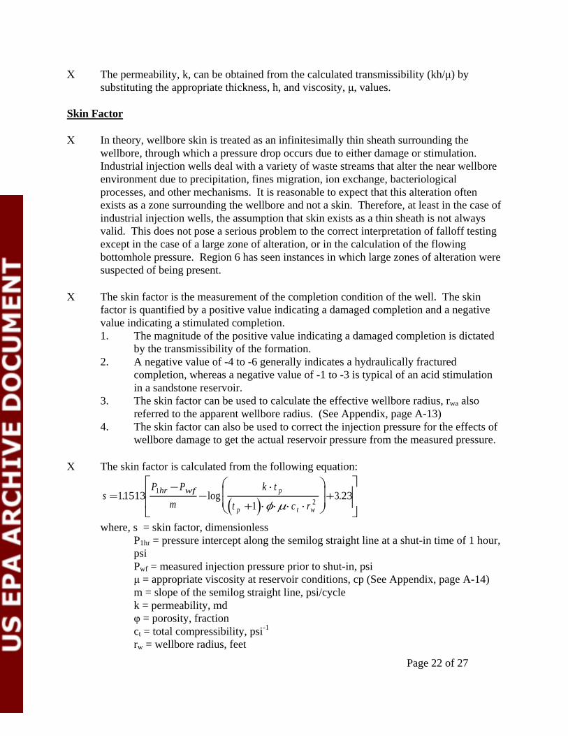
Skin Factor

Χ In theory, wellbore skin is treated as an infinitesimally thin sheath surrounding the wellbore, through which a pressure drop occurs due to either damage or stimulation. Industrial injection wells deal with a variety of waste streams that alter the near wellbore environment due to precipitation, fines migration, ion exchange, bacteriological processes, and other mechanisms. It is reasonable to expect that this alteration often exists as a zone surrounding the wellbore and not a skin. Therefore, at least in the case of industrial injection wells, the assumption that skin exists as a thin sheath is not always valid. This does not pose a serious problem to the correct interpretation of falloff testing except in the case of a large zone of alteration, or in the calculation of the flowing bottomhole pressure. Region 6 has seen instances in which large zones of alteration were suspected of being present.

Χ The skin factor is the measurement of the completion condition of the well. The skin factor is quantified by a positive value indicating a damaged completion and a negative value indicating a stimulated completion. 1. The magnitude of the positive value indicating a damaged completion is dictated

by the transmissibility of the formation. 2. A negative value of -4 to -6 generally indicates a hydraulically fractured

completion, whereas a negative value of -1 to -3 is typical of an acid stimulation in a sandstone reservoir.

3. The skin factor can be used to calculate the effective wellbore radius, rwa also referred to the apparent wellbore radius. (See Appendix, page A-13)

4. The skin factor can also be used to correct the injection pressure for the effects of wellbore damage to get the actual reservoir pressure from the measured pressure.

Χ The skin factor is calculated from the following equation: ⎡ ⎛ ⎞ ⎤P −P k t⋅1hr wf ps =1.1513⎢ −log ⎜

2 ⎟⎟

+3.23⎥ + ⋅ ⋅ ⋅ ⋅r⎢ m ⎜ t 1 φ μ c ⎥

⎣ ⎝( p ) t w ⎠ ⎦ where, s = skin factor, dimensionless

P1hr = pressure intercept along the semilog straight line at a shut-in time of 1 hour, psi Pwf = measured injection pressure prior to shut-in, psi μ = appropriate viscosity at reservoir conditions, cp (See Appendix, page A-14) m = slope of the semilog straight line, psi/cycle k = permeability, md φ = porosity, fraction ct = total compressibility, psi-1

rw = wellbore radius, feet

Page 22 of 27

✓-

tp = injection time, hours Note that the term tp/(tp +Δt), where Δt=1 hr, appears in the log term. This term is usually assumed to result in a negligible contribution and typically is taken as 1 for large t. However, for relatively short injection periods, as in the case of a drill stem test (DST), this term can be significant.

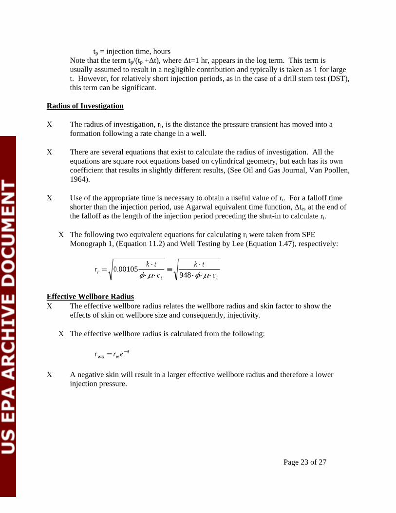
Radius of Investigation

Χ The radius of investigation, ri, is the distance the pressure transient has moved into a formation following a rate change in a well.

Χ There are several equations that exist to calculate the radius of investigation. All the equations are square root equations based on cylindrical geometry, but each has its own coefficient that results in slightly different results, (See Oil and Gas Journal, Van Poollen, 1964).

Χ Use of the appropriate time is necessary to obtain a useful value of ri. For a falloff time shorter than the injection period, use Agarwal equivalent time function, Δte, at the end of the falloff as the length of the injection period preceding the shut-in to calculate ri.

Χ The following two equivalent equations for calculating ri were taken from SPE Monograph 1, (Equation 11.2) and Well Testing by Lee (Equation 1.47), respectively:

k t⋅ k t⋅ ri = 0.00105 ≡φ μ⋅ ⋅c t 948 ⋅ ⋅φ μ⋅c t

Effective Wellbore Radius Χ The effective wellbore radius relates the wellbore radius and skin factor to show the

effects of skin on wellbore size and consequently, injectivity.

Χ The effective wellbore radius is calculated from the following:

−sr = r e wa w

Χ A negative skin will result in a larger effective wellbore radius and therefore a lower injection pressure.

Page 23 of 27

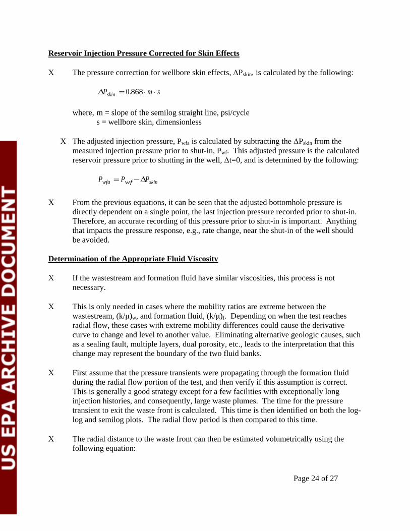
Reservoir Injection Pressure Corrected for Skin Effects

Χ The pressure correction for wellbore skin effects, ΔPskin, is calculated by the following:

ΔP = 0.868 ⋅m ⋅ sskin

where, m = slope of the semilog straight line, psi/cycle s = wellbore skin, dimensionless

Χ The adjusted injection pressure, Pwfa is calculated by subtracting the ΔPskin from the measured injection pressure prior to shut-in, Pwf. This adjusted pressure is the calculated reservoir pressure prior to shutting in the well, Δt=0, and is determined by the following:

P = P −ΔPwfa wf skin

Χ From the previous equations, it can be seen that the adjusted bottomhole pressure is directly dependent on a single point, the last injection pressure recorded prior to shut-in. Therefore, an accurate recording of this pressure prior to shut-in is important. Anything that impacts the pressure response, e.g., rate change, near the shut-in of the well should be avoided.

Determination of the Appropriate Fluid Viscosity

Χ If the wastestream and formation fluid have similar viscosities, this process is not necessary.

Χ This is only needed in cases where the mobility ratios are extreme between the wastestream, (k/μ)w, and formation fluid, (k/μ)f. Depending on when the test reaches radial flow, these cases with extreme mobility differences could cause the derivative curve to change and level to another value. Eliminating alternative geologic causes, such as a sealing fault, multiple layers, dual porosity, etc., leads to the interpretation that this change may represent the boundary of the two fluid banks.

Χ First assume that the pressure transients were propagating through the formation fluid during the radial flow portion of the test, and then verify if this assumption is correct. This is generally a good strategy except for a few facilities with exceptionally long injection histories, and consequently, large waste plumes. The time for the pressure transient to exit the waste front is calculated. This time is then identified on both the log-log and semilog plots. The radial flow period is then compared to this time.

Χ The radial distance to the waste front can then be estimated volumetrically using the following equation:

Page 24 of 27

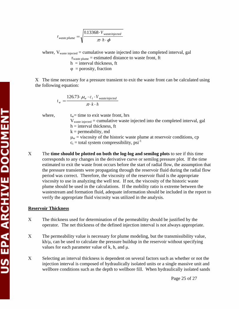
✓-0.13368 ⋅V wasteinjectedr = waste plume ⋅ ⋅hπ φ

where, Vwaste injected = cumulative waste injected into the completed interval, gal rwaste plume = estimated distance to waste front, ft h = interval thickness, ft φ = porosity, fraction

Χ The time necessary for a pressure transient to exit the waste front can be calculated using the following equation:

. ⋅μ c V126 73 ⋅ ⋅ w t wasteinjectedt w = π⋅ ⋅k h

where, tw= time to exit waste front, hrs Vwaste injected = cumulative waste injected into the completed interval, gal h = interval thickness, ft k = permeability, md μw = viscosity of the historic waste plume at reservoir conditions, cp ct = total system compressibility, psi-1

Χ The time should be plotted on both the log-log and semilog plots to see if this time corresponds to any changes in the derivative curve or semilog pressure plot. If the time estimated to exit the waste front occurs before the start of radial flow, the assumption that the pressure transients were propagating through the reservoir fluid during the radial flow period was correct. Therefore, the viscosity of the reservoir fluid is the appropriate viscosity to use in analyzing the well test. If not, the viscosity of the historic waste plume should be used in the calculations. If the mobility ratio is extreme between the wastestream and formation fluid, adequate information should be included in the report to verify the appropriate fluid viscosity was utilized in the analysis.

Reservoir Thickness

Χ The thickness used for determination of the permeability should be justified by the operator. The net thickness of the defined injection interval is not always appropriate.

Χ The permeability value is necessary for plume modeling, but the transmissibility value, kh/μ, can be used to calculate the pressure buildup in the reservoir without specifying values for each parameter value of k, h, and μ.

Χ Selecting an interval thickness is dependent on several factors such as whether or not the injection interval is composed of hydraulically isolated units or a single massive unit and wellbore conditions such as the depth to wellbore fill. When hydraulically isolated sands

Page 25 of 27

are present, it may be helpful to define the amount of injection entering each interval by conducting a flow profile survey. Temperature logs can also be reviewed to evaluate the intervals receiving fluid. Cross-sections may provide a quick look at the continuity of the injection interval around the injection well.

Χ A copy of a SP/Gamma Ray well log over the injection interval, the depth to any fill, and the log and interpretation of available flow profile surveys run should be submitted with the falloff test to verify the reservoir thickness value assumed for the permeability calculation.

Use of Computer Software

Χ To analyze falloff tests, operators are encouraged to use well testing software. Most software has type curve matching capabilities. This feature allows the simulation of the entire falloff test results to the acquired pressure data. This type of analysis is particularly useful in the recognition of boundaries, or unusual reservoir characteristics, such as dual porosity. It should be noted that type curve matching is not considered a substitute, but is a compliment to the analysis.

Χ All data should be submitted on a CD-ROM with a label stating the name of the facility, the well number(s), and the date of the test(s). The label or READ.Me file should include the names of all the files contained on the CD, along with any necessary explanations of the information. The parameter units format (hh:mm:ss, hours, etc.) should be noted for the pressure file for synchronization to the submitted injection rate information. The file containing the gauge data analyzed in the report should be identified and consistent with the hard copy data included in the report. If the injection rate information for any well included in the analysis is greater than 10 entries, it should also be included electronically.

Common Sense Check

Χ After analyzing any test, always look at the results to see if they “make sense” based on the type of formation tested, known geology, previous test results, etc. Operators are ultimately responsible for conducting an analyzable test and the data submitted to the regulatory agency.

Χ If boundary conditions are observed on the test, review cross-sections or structure maps to confirm if the presence of a boundary is feasible. If so, the boundary should be considered in the AOR pressure buildup evaluation for the well.

Χ Anomalous data responses may be observed on the falloff test analysis. These data anomalies should be evaluated and explained. The analyst should investigate physical causes in addition to potential reservoir responses. These may include those relating to the well equipment, such as a leaking valve, or a channel, and those relating to the data

Page 26 of 27

acquisition hardware such as a faulty gauge. An anomalous response can often be traced to a brief, but significant rate change in either the test well or an offset well.

Χ Anomalous data trends have also been caused by such things as ambient temperature changes in surface gauges or a faulty pressure gauge. Explanations for data trends may be facilitated through an examination of the backup pressure gauge data, or the temperature data. It is often helpful to qualitatively examine the pressure and/or temperature channels from both gauges. The pressure data should overlay during the falloff after being corrected for the difference in gauge depths. On occasion, abrupt temperature changes can be seen to correspond to trends in the pressure data. Although the source of the temperature changes may remain unexplainable, the apparent correlation of the temperature anomaly to the pressure anomaly can be sufficient reason to question the validity of the test and eliminate it from further analysis.

Χ The data that is obtained from pressure transient testing should be compared to permit parameters. Test derived transmissibilities and static pressures can confirm compliance with non-endangerment (Area Of Review) conditions.

Page 27 of 27

Appendix F

EPA Region 9 Step Rate Test Procedure Guidelines


APPENDIX F – Region 9 Step Rate Test Policy

For reference please refer to:

Society of Petroleum Engineers (SPE) Paper #16798, Systematic Design and Analysis of Step-Rate Tests to Determine Formation Parting Pressure

(This paper may be obtained from the SPE.)

Appendix G

Plugging and Abandonment Plans


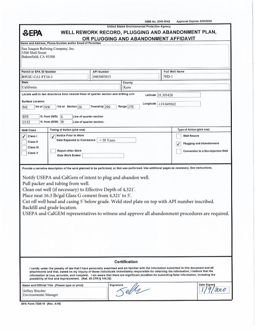
Notify USEPA and CalGem of intent to plug and abandon well. Pull packer and tubing from well. Clean out well (if necessary) to Effective Depth of 4,321'. Place neat 16.3 lb/gal Glass G cement from 4,321' to 5'. Cut off well head and casing 5' below grade. Weld steel plate on top with API number inscribed. Backfill and grade location. USEPA and CalGEM representatives to witness and approve all abandonment procedures are required.

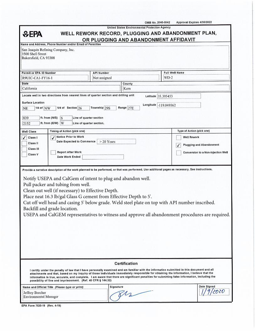
Notify USEPA and CalGem of intent to plug and abandon well. Pull packer and tubing from well. Clean out well (if necessary) to Effective Depth. Place neat 16.3 lb/gal Glass G cement from Effective Depth to 5'. Cut off well head and casing 5' below grade. Weld steel plate on top with API number inscribed. Backfill and grade location. USEPA and CalGEM representatives to witness and approve all abandonment procedures are required.

Appendix H

Operating Data


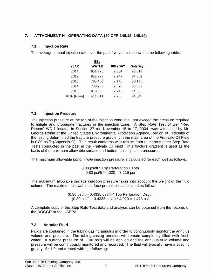
7. ATTACHMENT H - OPERATING DATA (40 CFR 146.12, 146.14)

7.1. Injection Rate The average annual injection rate over the past five years is shown in the following table:

BBL YEAR WATER BBL/DAY Gal/Day 2011 851,776 2,334 98,013 2012 822,299 2,247 94,362 2013 783,403 2,146 90,145 2014 739,239 2,025 85,063 2015 819,565 2,245 94,306

2016 (6 mo) 411,011 2,258 94,849

7.2. Injection Pressure The injection pressure at the top of the injection zone shall not exceed the pressure required to initiate and propagate fractures in the injection zone. A Step Rate Test of well “Red Ribbon” WD-1 located in Section 27 run November 15 to 17, 2004 was witnessed by Mr. George Robin of the United States Environmental Protection Agency, Region IX. Results of the testing determined the fracture pressure gradient in the main area of the Fruitvale Oil Field is 0.80 psi/ft (Appendix O). This result conforms with results from numerous other Step Rate Tests conducted in the past in the Fruitvale Oil Field This fracture gradient is used as the basis of the maximum allowable surface and bottom hole injection pressures.

The maximum allowable bottom hole injection pressure is calculated for each well as follows:

0.80 psi/ft * Top Perforation Depth 0.80 psi/ft * 4,020 = 3,216 psi

The maximum allowable surface injection pressure takes into account the weight of the fluid column. The maximum allowable surface pressure is calculated as follows:

(0.80 psi/ft – 0.4335 psi/ft) * Top Perforation Depth (0.80 psi/ft – 0.4335 psi/ft) * 4,020 = 1,473 psi

A complete copy of the Step Rate Test data and analysis can be obtained from the records of the DOGGR or the USEPA.

7.3. Annular Fluid Fluids are contained in the tubing-casing annulus in order to continuously monitor the annulus volume and pressure. The tubing-casing annulus will remain completely filled with fresh water. A surface pressure of ~100 psig will be applied and the annulus fluid volume and pressure will be continuously monitored and recorded. The fluid will typically have a specific gravity of ~1.0 and treated with the following:

San Joaquin Refining Company, Inc. Class I UIC Permit Application 9 PETROtech Resources Company

2% potassium chloride (KCl). Corrosion inhibitor (see above). Oxygen scavenger (sodium sulfite, hydrazine) Biocide (sodium chromate, mercuric chloride, silver nitrate, coco primary amine

acetate, coco trimethylene diamine, alkyl trimethyl quaternary ammonium chlorite, 1-phynyl-4, 4-dimethyl imidazoline, sodium tetrachlorphenate, acrolein, peracetic acid)

Nitrogen is used at the surface to maintain a constant pressure of approximately 100 psig on the annular fluid. The specific gravity of fluid is approximately 1.0.

These monitoring fluids are available through various commercial chemical suppliers and are often proprietary. The typical chemical composition of the annulus fluid is:

Material % Concentration Methanol 0.2 to 0.4 Alkylpyridine salts 0.02 to 0.06 Fatty quarternary NH4Cl 0.005 to 0.03 Potassium chloride (KCl) 1.0 to 3.0

7.4. Injection Fluid Characteristics Laboratory analytical results for injection fluid samples for calendar year 2016 are contained in Appendix E. The analytical data includes water quality information including the Title 22 metals, phenols, total dissolved solids, electrical conductivity, pH, fluoride, sulfate, chloride, potassium, sodium, magnesium. and calcium. Analysis is conducted by a state certified laboratory.

7.5. Source of Water The waste stream sent to the injection wells for disposal is the treated effluent of the wastewater treatment plant. No other waste streams are discharged to the injection wells.

San Joaquin Refining Company, Inc. Class I UIC Permit Application 10 PETROtech Resources Company

Documents

Appendices: UIC Permit R9UIC-CA1-FY16-1 · UIC Permit R9UIC-CA1-FY16-1 . APPENDIX C – EPA Reporting Forms Form 7520-8: Quarterly Injection WellMonitoring Report Form 7520-18: Completion