Appendix 1 Cartesian Tensor Analysis - Home - Springer978-1-4615-3110...554 Appendix 1. Cartesian Tensor Analysis X3, which may stand for Cartesian x, y, z or cylindrical r, 0, and

Appendix 1

Cartesian Tensor Analysis

Al.l ARE TENSORS FOR REAL?

Tensor analysis and calculus is a branch of mathematics that deals with coordinate transformation, and the appearance of the laws of physics in various coordinate systems. This appendix is a cursory review of the basics of tensor analysis. Additional reading is necessary for a fuller understanding. References listed at the end are only moderately complex since they discuss the application of tensors to elasticity theory.

Tensors are physically real quantities. They are a class of quantities which are more general than vectors. The fact that stress and strain are tensor quantities and not vectors gave rise to the name. The word tensor means tension.

Tensors use a notation that is intimidating to some. It is a system of subscript notation generalized to a great extent, so that a high degree of brevity is achieved. However, brevity is not its basic purpose. It is a way of transforming a set of quantities from one coordinate system to another. The expressibility of physical laws in tensor form is a guarantee of their coordinate independence and absoluteness. Fundamental laws of nature such as the laws of electromagnetism, conservation of energy, conservation of mass, etc. are expressible in tensor form. So is elasticity theory, which verifies its absoluteness. That is, elasticity theory is valid on earth and in space as well.

AI.2 THE SUBSCRIPT NOTATION

Instead on naming the coordinate axes as x, y, and z, we just label them "first," "second," and "third." The coordinates are denoted by Xl' x z, and

553

554 Appendix 1. Cartesian Tensor Analysis

X 3, which may stand for Cartesian x, y, z or cylindrical r, 0, and z, or any curvilinear u, v, and w. In this appendix, we stick to the Cartesian coordinates of different orientations and positions. Thus, coordinates are denoted by

Xi' (i = 1,2, and 3)

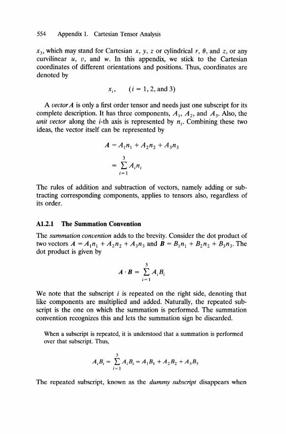
A vector A is only a first order tensor and needs just one subscript for its complete description. It has three components, AI' A 2 , and A 3. Also, the unit vector along the i-th axis is represented by ni. Combining these two ideas, the vector itself can be represented by

3

= " A·n· '-- I I

;=1

The rules of addition and subtraction of vectors, namely adding or subtracting corresponding components, applies to tensors also, regardless of its order.

A1.2.t The Summation Convention

The summation convention adds to the brevity. Consider the dot product of two vectors A = Aini + A 2nZ + A3n3 and B = Bini + B2nZ + B3n3. The dot product is given by

3

A·B = EAiBi ;= 1

We note that the subscript i is repeated on the right side, denoting that like components are multiplied and added. Naturally, the repeated subscript is the one on which the summation is performed. The summation convention recognizes this and lets the summation sign be discarded.

When a subscript is repeated, it is understood that a summation is performed over that subscript. Thus,

3

AiBi = LAiBi =AjBj +AzB2 +A3 B3 i= 1

The repeated subscript, known as the dummy subscript disappears when

Al.2 The Subscript Notation 555

the summation is performed. Any other symbol is just the same. Hence the name "dummy."

Matrices are two-dimensional arrays, and can be represented by two subscripts, the first one for the row number, and the second for the column. The matrix itself may represent a tensor or not. The rule of matrix multiplication is represented by

C ij = LAikBkj k

Using the summation convention, this can be written as

The multiplication of a matrix by a column vector is represented as

A1.2.2 The Kronecker Delta

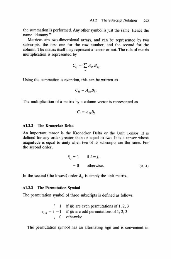
An important tensor is the Kronecker Delta or the Unit Tensor. It is defined for any order greater than or equal to two. It is a tensor whose magnitude is equal to unity when two of its subscripts are the same. For the second order,

if i = j,

=0 otherwise.

In the second (the lowest) order 8ij is simply the unit matrix.

A1.2.3 The Permutation Symbol

The permutation symbol of three subscripts is defined as follows.

if ijk are even permutations of 1, 2, 3 if ijk are odd permutations of 1, 2, 3 otherwise

(AU)

The permutation symbol has an alternating sign and is convenient in


calculating the determinant of a matrix, or the curl of a vector. This symbol is used wherever there is rotation.

The same equation can be expressed in subscript notation as,

Al.2.4 The Formal Definition of a Tensor

The important characteristic that identifies and defines a tensor is the rule it obeys under transformation of coordinates. Coordinates transform according to the rule

where Lij is the matrix of the direction cosines.

The matrix Lij is central to the tensor definition. If Aj are the components of a first order tensor in the x' coordinates,

and Ai are its components in the x coordinate system, then

(Al.2)

This rule, identical to the vector transformation, does not tell much about tensors in particular. Consider the second and higher order transformation rules. For second order tensors (which stress and strain are),

(A1.3)

(Al.4)

(A1.5)

The second and higher order transformations really define the tensor. The rule for the second order tensor transformation is identical to what we learned as the Mohr's circle. Higher orders are generalizations.

A1.2.S The Stress Strain, and Elastic Moduli Tensors-The Quotient Law

From Chapter 1, we have a definition of stress as the density of force distribution 1j on a small are dAi' The force distribution vector 1j is

Al.2 The Subscript Notation 557

referred to sometimes as the traction vector. The definition of stress given in Chapter 1 in terms of traction vectors may be written in tensor notation as

The fact that aij = Oji is a consequence of moment equilibrium of stress at a vanishingly small volume.

Strain as defined in Chapter 1 is not a tensor. However, the mathematical definition of strain is equivalent to halving the shear strains. The displacements u, v, and w may be denoted as U i ' (i = 1,2,3). In tensor notation, the definition of strain may be written in terms of displacements as

When i = j, the engineering and mathematical definitions of normal strains coincide, but not for shear strains. Also, the symmetry of strains is seen straightaway, since interchange of i and j leaves the definition unchanged.

Hooke's laws for isotropic materials can be expressed in tensor notation in terms of G and A (usually called Lame's constants).

This is identical to the six Equations 1.23 and 1.24. Stress and strains are tensors, because the rule of their transformation

conforms to that of tensors. Initially, knowing nothing about the way they are related, we may assume the strain €kl and stress aij are linearly related. Hence, we may write the generalized Hooke's law in the form

where the elastic moduli Eijkl is a fourth order tensor, which contracts to second order by multiplication and summation on the right side. There is no a priori reason to know that elastic moduli are tensors. The form of the equation relating them is the only clue. Guessing the higher order of the tensor from the form of the physical rules as above is called the quotient rule.

The four subscripts in three dimensions imply 34 = 81 components of


moduli. However, for three-dimensional orthotropic composites (which is the most general form for practical engineering purposes), the number of independent elastic constants reduces to only 9. As mentioned in Chapter 7, other physical principles such as symmetry, equivalence of left- and right-handed coordinate systems, etc. need to be exercised. Reference 2 is recommended in this context.

A1.2.6 Differentiation and Equilibrium Equations

Partial differential coefficients with respect to a coordinate is represented by a comma, followed by the coordinate index. Thus

However, if k = i or j, then a summation is indicated, III addition. Therefore,

Utilizing the notation, the equilibrium equations of Chapter 1 can be summarized by a single statement.

(i=I,2,3)

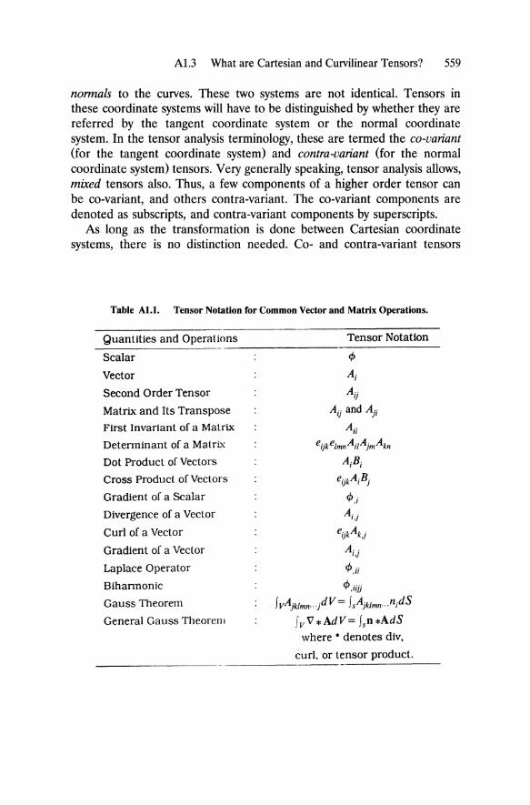
Furthermore, the identities listed in Table A1.1 may be verified.

AI.3 WHAT ARE CARTESIAN AND CURVILINEAR TENSORS?

Many text books in tensor analysis use the two terms "Cartesian" and "curvilinear" tensors. Many times, some knowledge of curvilinear coordinates and vector calculus in such coordinates is assumed.

What we discussed above are "Cartesian" tensors. The matrices Lij are the direction cosine matrices for transformation between Cartesian coordinates. If instead, we had a cylindrical or spherical coordinate system or any other system as our destination coordinate system, then the transformation matrix would change from point to point.

It is easy to expect that the local tangents to the coordinate curves will form the new coordinate axis. An equally valid system is the set of local

Al.3 What are Cartesian and Curvilinear Tensors? 559

nonnals to the curves. These two systems are not identical. Tensors in these coordinate systems will have to be distinguished by whether they are referred by the tangent coordinate system or the normal coordinate system. In the tensor analysis terminology, these are termed the co-variant (for the tangent coordinate system) and contra-variant (for the normal coordinate system) tensors. Very generally speaking, tensor analysis allows, mixed tensors also. Thus, a few components of a higher order tensor can be co-variant, and others contra-variant. The co-variant components are denoted as subscripts, and contra-variant components by superscripts.

As long as the transformation is done between Cartesian coordinate systems, there is no distinction needed. Co- and contra-variant tensors

Table AI.I. Tensor Notation for Common Vector and Matrix Operations.

Quantities and Operations Tensor Notation -------------------------------

Scalar

Vector

Second Order Tensor

Matrix and Its Transpose

First Invariant of a Matrix

Detenninant of a Matrix

Dot Product of Vectors

Cross Product of Vectors

Gradient of a Scalar

Divergence of a Vector

Curl of a Vector

Gradient of a Vector

Laplace Operator

Bihannonic

Gauss Theorem

General Gauss Theorem

A;

Aij

Aij and Aj;

A;;

e;jkelmnAi/AjmAkn

A;B;

e;jkA;Bj

cf>,;

A;,j

e;jkAk,j

A· 1,)

cf>,i;

cf>,;;jj

IVAjklmn .. -jdV= IsAjklmn ... n;dS

Iv V *AdV= Iso *AdS where • denotes diY,

curl. or tensor product.


represent one and the same set of components, and hence only subscripts are used throughout. Rigorous validation of the absoluteness of elasticity theory requires the use of curvilinear tensors.

References 1. Chou, P. C. and Pagano, N. J., Elasticity, Tensor, Dyadic and Engineering

Approaches, 1967, D. Van Nostrand Company, Inc., Princeton, N.J. 2. Agarwal, B. D. and Broutman, L. J., Analysis and Performance of Fiber Compos

ites, 2nd Edn. 1990, John Wiley & Sons, New York, NY.

Appendix 2

Methods in Beam Theory

Formulas for the deflection and stress in (statically determinate) beams are available as appendices and tables in several text books. See Reference 1 for the basic ones and Reference 2 for more complex formulas. The purpose of this appendix is to illustrate the use of the so-called superposition method for beams. The salient parameters needed in a beam problem are the bending moment (M), shear force (V), deflection (8), and slope of the deflected shape «(}). All of these are related to distance x along the axis of the beam by linear differential equations.

The variables M, V, 8, () and consequently the bending stress u are alliineady additive. Thus, if two loads cause deflections 81 and 82 , acting separately, then they cause a deflection (81 + 82 ) acting concurrently. The only requirement is that the support conditions must remain same.

Nomenclature

f: Moment of area of cross section about its neutral axis z: Modulus of cross section = fly E: Young's modulus of the material M: Bending moment at a point R: Support reaction a: Bending stress 8,0: Deflection and slope of the beam

Example A2.1

Find the deflection at the center of a simply supported beam loaded on only one half of its span.

561

562 Appendix 2. Methods in Beam Theory

Case

2

3

4

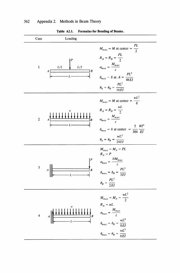
Table A2.1. Formulas for Bending of Beams.

Loading

L/2 r L/2 AI IB

I· L 1

"' JHH!HHHHB

I· L ·1

"'

'1111111111111 t· • L 1

PL Mmax = M at center = 2

PL RA =RB = 2

Mmax (J'max = -z-

WL2

Mmax = M at center = -8-

wL RA =RB = 2

Mmax (Tmax =-

Z

8max = 8 at center

wL3

°A = °B = 24El

Mmax = MA = PL

RA =P

(Tmax =--Z

PL3

8max = 8B = 3El

PL2

0=-B 2EI

WL2

Mmax =MA = 2 RA =wL

lTmax =--Z

wL4

8max = 8B = 8El

wL3

°max = °B = 6El

5 W/ 4

384 EI

Appendix 2. Methods in Beam Theory 563

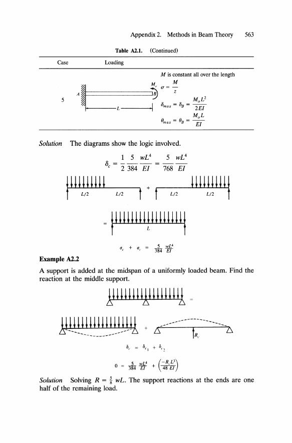
Table A2.1. (Continued)

Case Loading

M is constant all over the length

5

A i':~ M M .. ~=======~; u = -; M L2

I {) - {) - _0_

I-----L -----I. max - B - 2EI

MoL ()max = ()B = EI

Solution The diagrams show the logic involved.

1 5 wL4 5 WL4 8 =---=--

c 2 384 EI 768 EI

jllllllill Ll2 L/2 Ll2

1I1111111j Ll2

jllllllll!llllllllj

Example A2.2

A support is added at the midspan of a uniformly loaded beam. Find the reaction at the middle support.

1UJ!} 111111l}JJJ!1 ---------

5 wL4 (-ReO) o = 384 ET + \ 48 EI

--------6

Solution Solving R = % wL. The support reactions at the ends are one half of the remaining load.

564 Appendix 2. Methods in Beam Theory

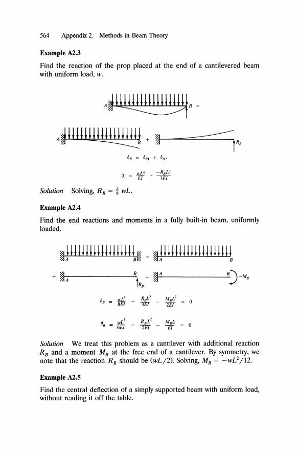
Example A2.3

Find the reaction of the prop placed at the end of a cantilevered beam with uniform load, w.

AJ~,

A~ II III III ~ + ~----==----=------'rB

Solution Solving, RB = ~ wL.

Example A2.4

Find the end reactions and moments in a fully built-in beam, uniformly loaded.

+ ~~ ____________ ~B ~rA--------------~~~-M8 ~A t + ~ ~

R8

Solution We treat this problem as a cantilever with additional reaction RB and a moment MB at the free end of a cantilever. By symmetry, we note that the reaction RB should be (wLI2). Solving, MB = -wL2/12.

Example A2.S

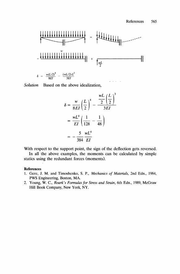
Find the central deflection of a simply supported beam with uniform load, without reading it off the table.

References 565

w

=UH!HHUHHHH~ + c-------~ t wL 2

4 3 {, _ w(L!2) _ (wL!2) L

- 8ifI ----w.I

Solution Based on the above idealization,

W (L)4 0= 8EI "2

~(~r 3EI

5 wL4

384 EI

With respect to the support point, the sign of the deflection gets reversed. In all the above examples, the moments can be calculated by simple

statics using the redundant forces (moments).

References 1. Gere, J. M. and Timoshenko, S. P., Mechanics of Materials, 2nd Edn., 1984,

PWS Engineering, Boston, MA. 2. Young, W. c., Roark's Formulas for Stress and Strain, 6th Edn., 1989, McGraw

Hill Book Company, New York, NY.

Appendix 3

Laplace Transforms

A3.1 DEFINITION

The Laplace transform is a mathematical technique for transforming differential equations into algebraic equations. Usually, time dependent differential equations are transformed by this process into algebraic equations in a dummy variable s, whose physical meaning is undefined. As such it is a very useful tool for solving problems involving rate processes.

Let t(t) be a given function for all t ~ O. Its Laplace transform ..21t(t )], denoted by j(s), is defined as,

if j(s) exists.

Conversely, if ..21t(t)] = j(s), then the inverse transform restores t(t). It is written as y-l[j(S)] = t(t). The technique of inverse transformation of j(s) is simply to use a few properties of Laplace transforms, reduce it to well known standard forms, and then to look up a table of transforms. This procedure is the engineer's approach, however, and not the mathematician's.

A3.2 TRANSFORMS OF ELEMENTARY FUNCTIONS

Taking transforms is simply an exercise in integral calculus. A few examples are listed below. Many others are given in Table A3.I at the end of this appendix.

566

A3.2 Transforms of Elementary Functions 567

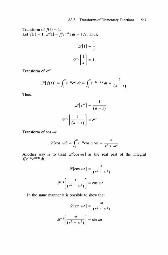
Transform of J(t) = 1. Let J(t) = 1. 2'[1] = f;e- S!l dt = l/s. Thus,

1 2'[1] = -

s

Transform of eat.

Thus,

00 00 1 2'[f(t)] = { e-steat dt = { e-(s-a)t dt = ---

Jo Jo (a - s)

1 2'[e at ] = --

(a - s)

y-l [ 1 ] = eat (a - s)

Transform of cos wt.

00 s ..2"[cos wt] = ( e-stcos wtdt = 2 2

Jo s + w

Another way is to treat 2'[cos wt] as the real part of the integral f;e-ste(iwt) dt.

s 2'[cos wt] = (2 2

S + w )

y-l [ 2 S 2 ] = cos wt (s + w )

In the same manner it is possible to show that

w ..2"[sin wt] = 2 2

(s + w )

yl[ (S2: W2)] = sin wt

568 Appendix 3. Laplace Transforms

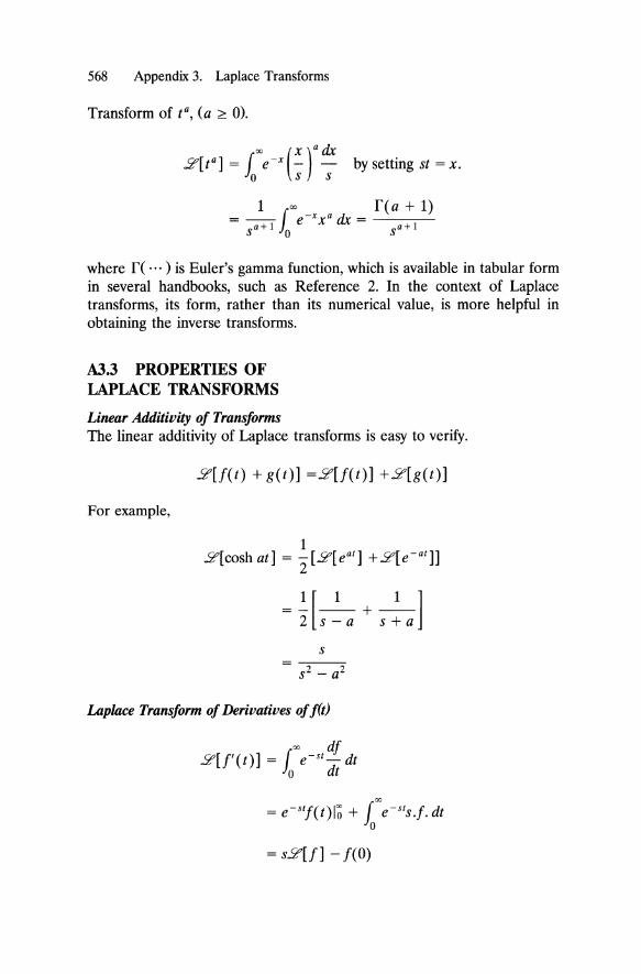
Transform of ta, (a ~ 0).

where f( ... ) is Euler's gamma function, which is available in tabular form in several handbooks, such as Reference 2. In the context of Laplace transforms, its form, rather than its numerical value, is more helpful in obtaining the inverse transforms.

A3.3 PROPERTIES OF LAPLACE TRANSFORMS

Linear Additivity of Transforms The linear additivity of Laplace transforms is easy to verify.

2[f(t) + get)] =2[f(t)] +2[g(t)]

For example,

s

Laplace Transform of Derivatives of f(t)

00 df 2[f'(t)] = 1 e- st _ dt

o dt

= s2[f] - f(O)

A3.3 Properties of Laplace Transforms 569

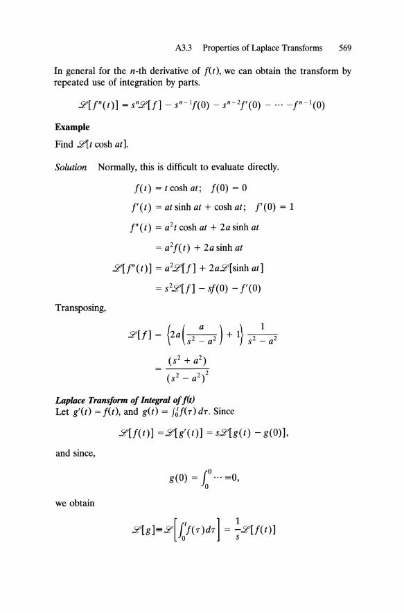
In general for the n-th derivative of J(t), we can obtain the transform by repeated use of integration by parts.

Example

Find 21t cosh at].

Solution Normally, this is difficult to evaluate directly.

Transposing,

J(t) = t cosh at; J(O) = 0

['(t) = at sinh at + cosh at; ['(0) = 1

f"(t) = a2t cosh at + 2a sinh at

= a2J(t) + 2a sinh at

2'[f"(t)] = a22'[f] + 2a2'[sinh at]

= s22'[ f] - sJ(O) - [' (0)

..2"[f] = {2a( 2 a 2) + I} 2 1 2 S -a s -a

(S2 + a2) 2

(S2 - a2)

Laplace Transform of Integral of f(t) Let g'(t) = J(t), and get) = fci!(r) dr. Since

2'[f(t)] =2'[g'(t)] = s2'[g(t) - g(O)],

and since,

we obtain


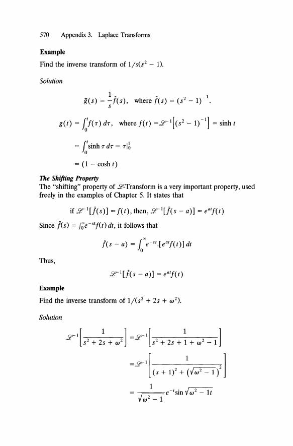
Example

Find the inverse transform of l/s(s2 - 1).

Solution

1 - 1 g(S) = -f(s), where !(s) = (S2 - 1) - .

s

it . 1 = smhrdr=rlo

o

= (1 - cosh t)

The Shifting Property The "shifting" property of 2-Transform is a very important property, used freely in the examples of Chapter 5. It states that

if y-l[f(S)] = f(t), then, y-l[f(S - a)] = eatf(t)

Since !(s) = J;e-stf(t) dt, it follows that

Thus,

Example

Find the inverse transform of 1/(s2 + 2s + w2).

Solution

References 571

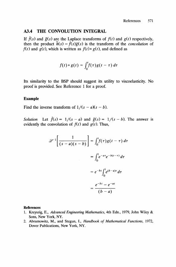
A3.4 THE CONVOLUTION INTEGRAL

If j(s) and g(s) are the Laplace transforms of !(t) and g(t) respectively, then the product h(s) = !(s)g(s) is the transform of the convolution of !(t) and g(t), which is written as !(t) * g(t), and defined as

!(t)*g(t) = [!(T)g(t- T)dT o

Its similarity to the BSP should suggest its utility to viscoelasticity. No proof is provided. See Reference 1 for a proof.

Example

Find the inverse transform of l/(s - aXs - b).

Solution Let !(s) = l/(s - a) and g(s) = l/(s - b). The answer is evidently the convolution of !(t) and g(t). Thus,

(b - a)

References 1. Kreyszig, E., Advanced Engineering Mathematics, 4th Edn., 1979, John Wiley &

Sons, New York, NY. 2. Abramowitz, M., and Stegun, I., Handbook of Mathematical Functions, 1972,

Dover Publications, New York, NY.


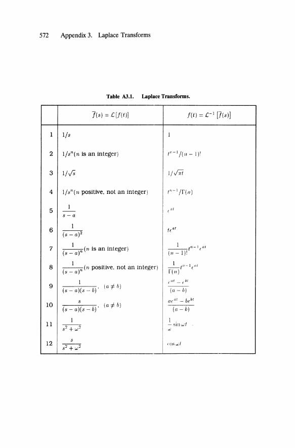
Table AJ.1. Laplace Transforms.

/(s) = [[f(t)l .r(t) = [-I [/(s)]

1 l/s

2 l/sn(n is an integer)

3 1/0

4 l/s"(11 positive, not an integer)

5 1

--s-o

6 1

(s - 0)2

1 7 -( --)-n (11 is an integer)

s-o

8 1

---. (n positive. not an integer) (8 - 0)"

9 1

(0 i- h) (s - o)(s - b)'

10 s

(a i- b) (s - a)( 8 - b) ,

11 1

s2 + w2

12 s

-,-, --0

s- + (;,r

I/J;i

1,,-I/f(lI)

1 n-I at ---t f (11 - 1)'

1 t,,-1 "I --. e ['( 11 )

(a - h)

(a - b)

1 . - Sill wi W

(·os .... :1

References 573

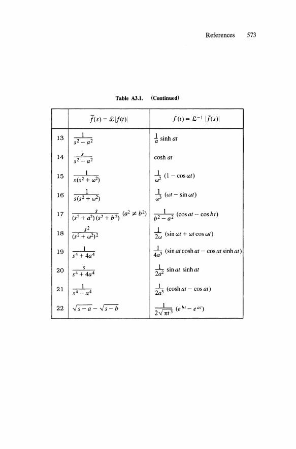
Table A3.1. (Continued)

l(s) = £IJ(t)1 J(t) = £-1 IRs)1

13 1 ~ sinh at s2 - a 2

14 s cosh at s2 - a 2

15 1 1 s(s2 + w2)

"2 (1- coswt) w

16 1 ~ (wt - sin wt)

s(s2 + w2) w

17 s (a2 ,c. b 2) b2~a2 (cosat-cosbt) (s2 + a2) (s2 + b 2) ,

18 s2 1 .

(s2 + w2)2 2w (sm wt + wtcos wt)

19 1 4!3 (sin at cosh at - cos at sinh at) s4 + 4a 4

20 s 2!2 sin at sinh at S4 + 4a 4

21 _1_ 2!3 (cosh at - cos at) S4 - a 4

22 ~-~ 1 ~ (ebt-e at )

2 trt 3

Appendix 4

Stress Intensity Factors for a Few Cases

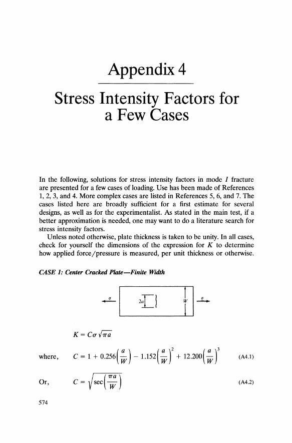
In the following, solutions for stress intensity factors in mode I fracture are presented for a few cases of loading. Use has been made of References 1,2,3, and 4. More complex cases are listed in References 5, 6, and 7. The cases listed here are broadly sufficient for a first estimate for several designs, as well as for the experimentalist. As stated in the main test, if a better approximation is needed, one may want to do a literature search for stress intensity factors.

Unless noted otherwise, plate thickness is taken to be unity. In all cases, check for yourself the dimensions of the expression for K to determine how applied force/pressure is measured, per unit thickness or otherwise.

CASE 1: Center Cracked Plate-Finite Width

-L-I '-----2L_1 ---I---J! I ~ K = C(T'/7Ta

where, C = 1 + O.256( ~ ) - 1.152( ~ r + 12.200( ~ r (A4.1)

Or, (A4.2)

574

Appendix 4. Stress Intensity Factors for a Few Cases 575

1 Or, C = ---;====-

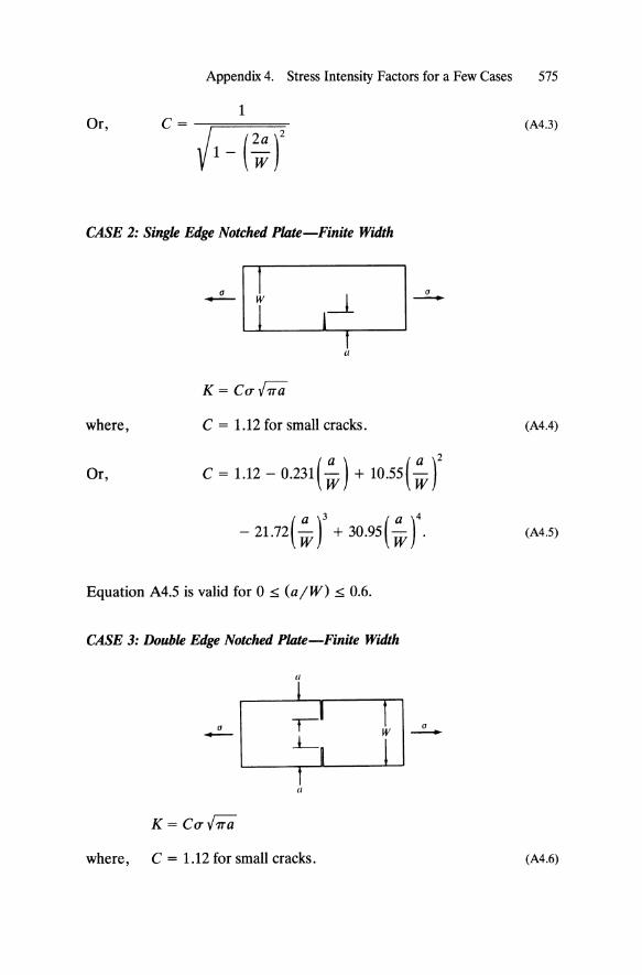
/1- (~ r CASE 2: Single Edge Notched Plate-Finite Width

where,

u -

K=Cuhra

1I

C = 1.12 for small cracks.

u -

Or, C = 1.12 - 0.231( ~ ) + 10.55 ( ~ r - 21.72 ( ~ r + 30.95 ( ~ r.

Equation A4.5 is valid for 0 ~ (a jW) ~ 0.6.

CASE 3: Double Edge Notched Plate-Finite Width

u -

K=Cuhra

1I

1I

where, C = 1.12 for small cracks.

u -

(A4.3)

(A4.4)

(A4.S)

(A4.6)

576 Appendix 4. Stress Intensity Factors for a Few Cases

Or, ( a) - 1 /2 [ ( a ) ( a )2 C = 1 - W 1.122 - 0.561 W - 0.205 W

+ 0.471 ( ~ r -0.190( ~ n (A4.7)

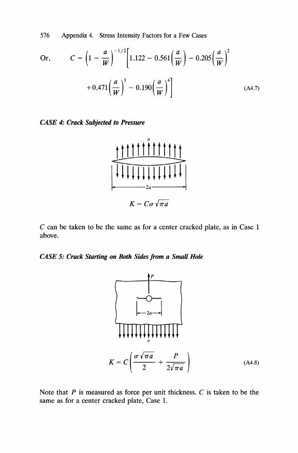
CASE 4: Crack Subjected to Pressure

(J

t t t t t t t t t t t t t <::::::: :=:::>-

~2~~ K = CO' V7Ta

C can be taken to be the same as for a center cracked plate, as in Case 1 above.

CASE 5: Crack Starting on Both Sides from a Small Hole

r (J

K=C +--( 0' (ii(i p)

2 2V7Ta (A4.8)

Note that P is measured as force per unit thickness. C is taken to be the same as for a center cracked plate, Case 1.


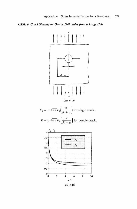
CASE 6: Crack Starting on One or Both Sides from a Large Hole

a

Itt t t t t t t I

~ ~ I

a

Case 6 (a)

KI = (J''; 'TT'a FI (_a_ ) for single crack. R +a

K = (J''; 'TT'a F2 (_a_) for double crack. R +a

0.5

o~--~--~--~----~--~

o 2 4 6 8 10 (aIr)

Case 6 (b)


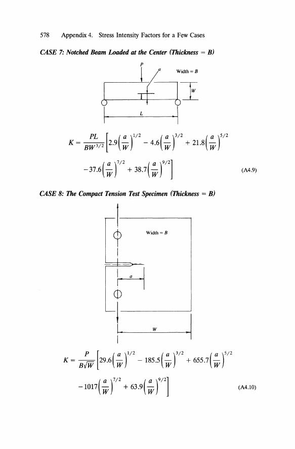
CASE 7: Notched Beam Loaded at the Center (Thickness = B)

p

1 ~'iJi I. L .\

K = B;~/2 [2.9(~ f/2 - 4.6( ~ f/2 + 21.8( ~ f/2

( a )7/2 ( a )9/2] -37.6 W + 38.7 W (A4.9)

CASE 8: The Compact Tension Test Specimen (Thickness = B)

1 cp Width = B

i

H CD

j

·1 I • w

I

p [ ( a )1/2 ( a )3/2 ( a )5/2 K = BIW 29.6 w - 185.5 W + 655.7 W

( a )7/2 ( a )9/2] -1017 W + 63.9 W (A4.1O)


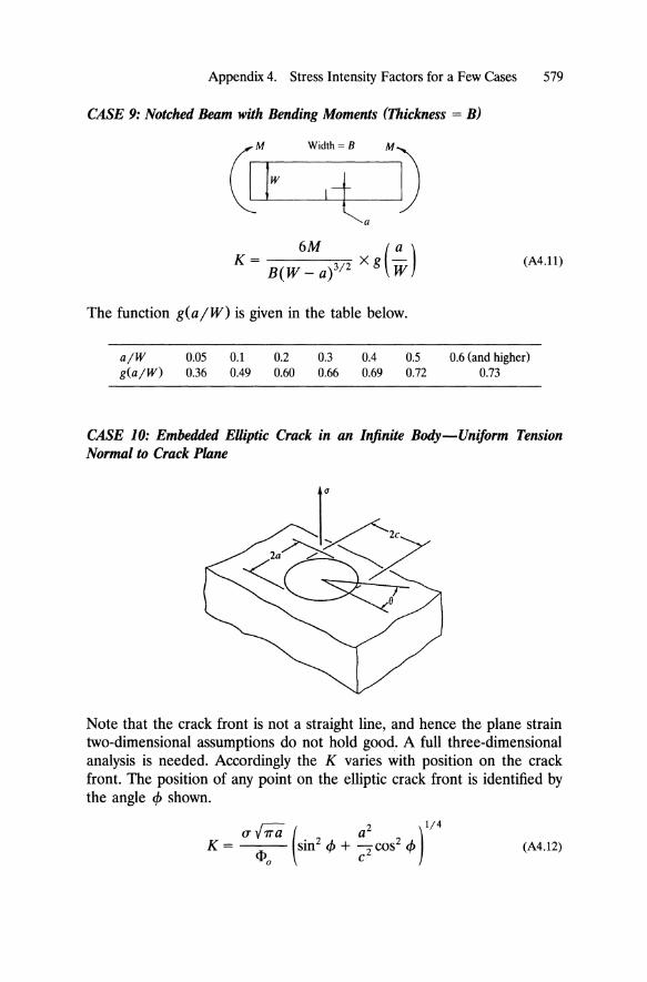
CASE 9: Notched Beam with Bending Moments (Thickness = B)

(A4.11)

The function g(a /W) is given in the table below.

a/W 0.05 0.1 0.2 0.3 0.4 0.5 0.6 (and higher) g(a/W) 0.36 0.49 0.60 0.66 0.69 0.72 0.73

CASE 10: Embedded Elliptic Crack in an Infinite Body-Uniform Tension Normal to Crack Plane

Note that the crack front is not a straight line, and hence the plane strain two-dimensional assumptions do not hold good. A full three-dimensional analysis is needed. Accordingly the K varies with position on the crack front. The position of any point on the elliptic crack front is identified by the angle 4> shown.

~ 2 1/4 aV7Ta( a )

K = <1>0 sin2 4> + c2 cos2 4> (A4.12)


In the above, the parameter CPo is the so-called elliptic integral defined by

[ ( 2 2 ) ]1/2 1T/2 C - a 4>0 = fa 1 - C2 sin2 () d() (A4.13)

This function is available in tabular form in several mathematical handbooks. Handbook of Mathematical Functions by Abramowitz and Stegun (Dover) is one such reference. More often its square Q = 4>; is used in some equations in the form

The function Q-called the Flaw Shape Parameter-is presented in Figure 6.22 for convenience.

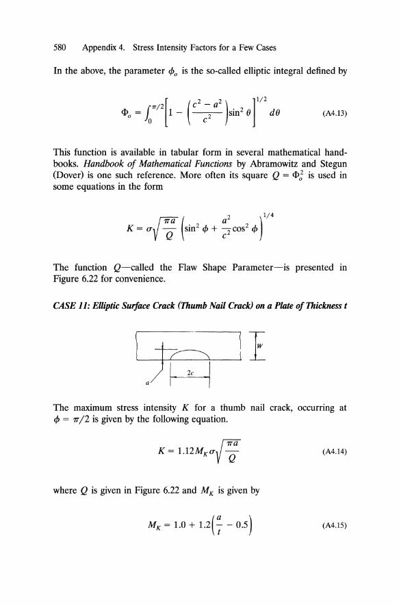
CASE 11: EUiptic Surface Crack (Thumb Nail Crack) on a Plate of Thickness t

The maximum stress intensity K for a thumb nail crack, occurring at cp = 7T /2 is given by the following equation.

(A4.14)

where Q is given in Figure 6.22 and M K is given by

(A4.15)


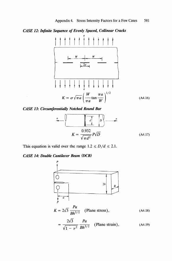
CASE 12: Infinite Sequence of Evenly Spaced, CoUinear Cracks a

tttiltltttttt

( W 1Ta )1/2

K = (r/1Ta -tan-1Ta W

CASE 13: CircumferentiaUy Notched Round Bar

0.932 In K= --PvD

V1Td 2

-

This equation is valid over the range 1.2 ~ D / d ~ 2.1.

CASE 14: Double Cantilever Beam (DCB) p

p

Pa K = 2/3 Bh3/ 2 (Plane stress),

2/3 Pa -;===7 -- (Plane strain), Jt - ,,2 Bh 3/ 2

(A4.16)

(A4.17)

(A4.18)

(A4.19)


CASE 15: Arc-Shaped Specimen

(/

w

x

p--+-

K= B~[1+1.54(~)+0.50(~)] (A4.20)

where,

(a) [ ( a )1/2 ( a )3/2 ( a )5/2 f W = 18.23 W - 106.2 W + 389.7 W

(A4.21)

( a )7/2 ( a )9/2] -582.0 W + 369.1 W


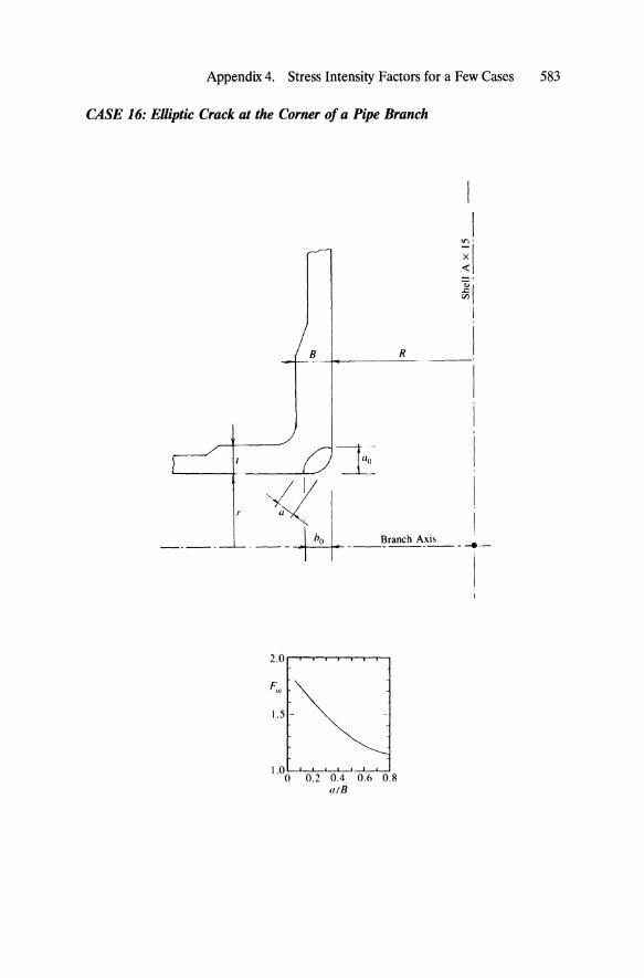
CASE 16: Elliptic Crack at the Corner of a Pipe Branch

B -+-___ R_

I I

~I ~I

I

I ~--'

I I ,

~~G_-=E~ !

, '~ I . --U ___ ~r_an_ch_A!_is_ -_t�-I

1.5 -

1.00 0.2 0.4 0.6 0.8 alB


For pressure containers of cylindrical shape and with branch pipes, it is known that cracks in the longitudinal plane (that is, those subjected to the full hoop stress) are the critical ones. They are located in otherwise high stress areas too, namely the junction of the branch pipe and the vessel. The solution for K for such cases is very important in pressurized container designs.

(A4.22)

In the above equation (Th stands for the hoop stress in the vessel. The parameter Fm is given in the adjoining figure.

References 1. Barsom, J. M. and Rolfe, S. T., Fatigue and Fracture Control in Structures, 2nd

Edn. 1987, Prentice Hall Inc., Englewood Cliffs, NJ. 2. Broek, D., Elementary Engineering Fracture Mechanics, 3rd Edn., 1982, Martinus

Nijhoff Publishers, Boston, MA. 3. Ewalds, H. L. and Wanhill, R. J. H., Fracture Mechanics, 1984, Co-published by

Edward Arnold and Delftse Uitgevers Maatschappij, Delft, Netherlands. 4. Paris, P. C. and Sih, G. c., ASTM STP 381, American Society for Testing and

Materials, 1964, Philadelphia, P A. 5. Sih, G. c., Handbook of Stress-Intensity Factors-Stress Intensity Factor Solutions

and Formulas for Reference, 1973, Institute of Fracture and Solid Mechanics, Lehigh University, Bethlehem, P A.

6. Rooke, D. O. and Cartwright, D. J., Compendium of Stress Intensity Factors, 1974, Her Majesty's Stationery Office, London.

7. Tada, H., Paris, P. c., and Irwin, G. R., The Stress Analysis of Cracks Handbook, 1973, Del Research Corporation.

Index*

ABAQUS, 451 Abstract elements, in FEM, 463 Adhesive bonding, rotating components, 114,

115 ADINA, 451 Aligned fiber reinforcement, 356 American Water Works Association, 89 ANSYS, 451 Argyris, J. H., 451 ASKA,451 Assembly of stiffness matrix, 482-485

for shared nodes, 485 ASTM

D-2344,443 D-790,79 D-790, see also Beams, commentary on

flexural testing F845, fittings, 126 requirements on K[c specimens, 321

Attenuation parameter, beta, 120 AWWA, see also American Water Works

Association C950-88,89

Axisymmetric shells, 116 membrane stresses in, Table 2.3, 117,

118

Back substitution, see Gauss elimination method example

Band storage, 496 Bandwidth, 486

minimization of, 496 Bauschinger effect, 152, 153 Beam theory, limitations of, 74 Beams, 66

commentary on flexural testing, 76 criteria for long beams, 74 made of nonlinear materials, 76 see also Euler beam theory statically determinate, 66 statically indeterminate, 66

Bending moments in shells, 119 vis a vis in pipes, 119n

Bezier curves, 525 Bezier surfaces, 527 Boltzmann's superposition principle, 206 Boolean operations, 527-529 Boundary condition, application of, 489, 490

interactive application, 531 BSP, see also Boltzmann's superposition

principle as integral representation, 206 derivation, 231-233

'References to specific matrices appear after the letter z.

585

586 Index

BSP (continued) for strain input history, Example 5.7,

236,237 for stress input history, Example 5.8,

238-240 to predict effects of cycling, 235, 236 to predict viscoelastic behavior, 233-235

Buckling, eigenvalue, Table 1.1, 5 of cylinders, 124 factor of safety, see FOS non-linear, Table 1.1, 5 strength of plastic components, Table

4.1,173 types of, 181

Bulk modulus, 149

CAD, see Computer Aided Design CAD files, cleanup, 533 CAD-to-FEM interface, 453 Cartesian tensors, 558 Cauchy, A. L., 16, 17 Centrifugal force, 111 Cheung, Y. K., 451 Choice of (FEM) elements, Figure 8.3,

460-462 Chopped fibers, random orientation, 363 Clough, R. W., 451 Compatibility, in elasticity, 44 Compatibility, equations, derivation of, 45 Complex compliance, 225 Complex modulus, 225 Composite wedge elements, 535 Composites, 342

balanced, 344 compliance matrix, 347 factors affecting properties, 355 material coordinate system, 344

Composites mathematical moduli, 349 micromechanics of, 354-371 orthotropic of, 344 quasi-isotropic, 344 specific moduli of, 346 specific strengths of, 346 stiffness matrix of, 349 strengths in material axes, 389 types of failure, 389-390

Computer Aided Design, 453 Considier, condition for instability, 148

Considier construction, 147 Constancy of volume, in yielding, 146 Constraint factor, 319 Contained plasticity, 323 Convolution integral, 571 Correspondence principle, 242-245

applications of, 247-251 in 3-dimensions, 246

COSMOS 7, 451 Coupled problems, 543

examples of, 172 Coupling constants of composites, meaning,

383-386 Courant, R., 450 Crack growth, catastrophic, 169 Crack initiation, 328 Crack propagation, cycle-dependent, Table

1.1,5 Crack propagation, time-dependent, Table

1.1,5 Crack tip opening displacement, 278 Crack tip plasticity, 317 Craze, a stress criterion for, 330

cusp shape as proof of Dugdale correction,329

porosity in, 164, 328 Craze stress, 329 Crazing, 145,328

micromechanism, 328 Creep, 3, 201

of standard viscoelastic model, 211 Creep buckling, 173 Creep compliance, 203

fully relaxed, 203 unrelaxed, 203

Creep, factor of safety on, see FOS Creep, linear, definition, 202 Creep modulus, methods for determination

of, 270 Creep strains, transient, 6 CTOD, see Crack tip opening displacement CTOD, as a fracture criterion, 287

for time dependent crack propagation, 335

Curves, in FEA modeling, 524, 525 Curvilinear tensors, 559

Degree of freedom, 454 Delrin, 148n

Design by analysis, 168 by rules, 168 causes of uncertainties, 170-74

Design rules, for long term, 268 Differentiation of tensors, 558 Diffusion problems, 450 Discontinuity, calculation of stresses at, 129 Discontinuity, structural, concept of, 127 Discontinuity, structural, use in design, 130 Displacement controlled problems, 47

influence on FOS, 179, 180 properties of, 92

Displacement vector, global, 458 Display of graphics, 529, 530 Distortion strain energy, 152 Distortion strain energy, see also Von Mises

criterion Do's and dont's, FEA, 531-542 DOF, see also Degree of freedom

per node, 454, 455 Double cantilever specimen, 291 Double torsion specimen, 291 Dugdale's correction for K1 , 325, 326

Effective length, in ASMEj ANSI Band PV Code, 123

Effective length, of a cylindrical shell, 122 Effectiveness, of ribs at a distance, 124 Eigenvalues, equal, see Principal stress, equal Elastic modulus tensor, 557, 558 Elasticity matrix, see [D] matrix Elasticity, theory of, 7, 64

equations, in polar coordinates, 97 Element

aspect ratios, good and poor, 539 connectivity, 459 coordinate system, 536 load vector, calculation of, 479-482 population density, 524 technology, 457 topology, 459 types, Figure 8.3, 460-462

Engineering moduli of plies, calculation of, 376

Environmental stress cracking, 328 Equations, bending of a laminate, 409-411 Equilibrium

equations, 19

Index 587

of forces and moments on a laminate, 412-414

problems, 450 of stresses at a point, 17

Euler, L., 64 Euler beam theory, 64 Expansion stress, 196 Extension ratio, 146 Extensive quantities, 16

Factor of safety, 174 applied to composite ply, 398

Failure criteria for composites for composites, 402-407 examples, 392-398 maximum strain criterion, 403 maximum stress criterion, 402 most restrictive, 405-407 Tsai-Hill criterion, 404 Tsai-Wu criterion, 405

Failures relation to stress categories, 187-191 various modes of, 169

Fatigue, 169, 332 crack propagation, 331 loading, Factor of safety on, see FOS

FCP, see Fatigue crack propagation FEA, see Finite element analysis FEA, steps involved, Table 8.1, 458 FEM, see Finite element method Fiber diameter, 342 Fibrils, 164, see also Crazing Findley's constants, 259

use of 259-265 Finite difference, 455 Finite element analysis, 452 Finite element method, 450 Finlayson, B. A., 457 First ply failure of laminates, 430 Flexibility matrix, 94 Fluid flow problems, 450 Force, body, 18 Forward reduction, see Gauss elimination

method, example FOS, see also Factor of safety, 174

based on severity of consequences of failure, 183

basis for, 183, 184 for buckling, 180, 181

588 Index

FOS (continued) for creep problems, 178, 179 for fatigue loading, 178 for local buckling, 182 for nonlinear material behavior, 179 for normal and overload conditions, 185 on short term strength, 175 on stiffness, 176 sizes of, for various conditions, Table

4.2,176 sizes of, for various conditions, 175-83 for thermal stress, intermittent, 177, 178 for thermal stress, sustained, 177

Fourier transforms use in rheological testing, 271, 272 use of, 223

FPF, see also First ply failure as the beginning of failure, 431 load calculation, examples, 432, 433 safety factor for, 431 strength of laminates, 430

Fracture, the three modes, 278, 279 Fracture criteria, general comments, 288 Fracture toughness, 2

plane strain, KIe , 285 Frontal solver, 498

G and crOD, relation, 327 G and I relation, 294, 295 G and K relation, 292, 294 G, for distributed loads, 291-292 Gauss elimination method, example, 490,

491-494,495 Gauss points, 510, 511 Gauss quadrature, 510, 513-514 Ge as a fracture criterion, 282

for a cracked body, 281 measurement of, 289-290 specimens of constant value, Figure 6.9,

291 Gradient matrix, see [B] matrix.

Halpin-Tsai formulas, 356, 365, 369 Heat conduction problems, 450 Helmholtz equation, 456 Hertzberg, R. W., 332 Hidden line removal, in FEM, 502 Hooke's law, 19, 20

for orthotropy, 345 inverted equations, 20 matrix form, 28

Hrenikoff, A, 450 Hydrostatic stress, sensitivity of materials to,

158 Hygroscopic coefficient, of laminates, 438 Hygrothermal coefficients

apparent, 442 definition of, 439

Hygrothermal effects, 437 Hygrothermal stresses, derivation, 439, 440

I/O operations, 452 Impact, 71

of bumpers, 71-72 energy absorption in, 73 kinetic energy of, 72

In-core procedures, 452 Instability problems, 450 Intensive quantities, 16 Inter-element compatibility, 469, 519 Interactive input, 452 Interlaminar shear

strength, 443 stress, 443

Interpolation functions, 464 calculation of, 468 computer coding, 470-472 forms of, 465 properties of, 469

Inverse approach, as a solution technique, 132

Irons, B. M., 451 Irwin's correction for KJ> 324 Isochronous curves, 202 Isoparametric elements, 503

linear quadrilateral, 508 linear triangle, 505 quadratic quadrilateral, 509 quadratic triangle, 507

Isotropy, see Exercise 1.23, 60 transverse, 347

J-Integral, 278 statement, 285-286

Jacobian determinant, 505 JIe , as a fracture criterion, 286

Keypoints, in FEA modeling, 524, 525 K1c' stress intensity factor, 278

arc-shaped specimen, 582 calculation of, 296, Appendix-4, 574 center cracked plate, 574 circumferential notched bar, 581 compact tension specimen, 578 crack(s) starting from a large hole, 577 cracked beam, moments, 579 cracked beam, central load, 578 for a crack in infinite plate, 297 cracks starting from a small hole, 576 double cantilever beam, 581 double edge crack, 575 elliptic crack at pipe branch, 583 for a few cases, 296-298 for line load on a crack face, 298 infinite sequence of cracks, 581 plane embedded elliptic crack, 579 pressurized crack faces, 576 properties of, 284 single edge crack, 575 superposition, examples, 298, 299-304 thumb nail crack, 580 as yield-or-break index, 312

K 1c ' ASTM Draft Standard for, 285 examples of non-dimensional form,

308-313 for a few materials, Table 6.1, 306 in light weight designs, 317 use in defect tolerant designs, Table

6.1,306 Kronecker delta, 555

Laminate point, stress analysis of, 408 Laminate thickness, design of, 436 Laminates, 407

symmetric, motivation for, 427 Laplace equation, 456 Laplace transforms, 566

for common functions, Table A3.1, 572-573

of derivatives, 568-569 of integrals, 569 linear additivity, 568 properties of, 568-570 shifting property, 570 use in viscoelasticity, 240

Leak-before-break, Example 6.13,313-316

Index 589

LEFM (Linear Elastic Fracture Mechanics), 542

Levy-Mises criterion, 163 Life Prediction, by Paris law, 332

examples, 333 Linear elastic behavior, basis for SCF, Exer

cise 1.27,6 Lines, in FEA modeling, 524, 525 Load-controlled problems, 44

influence on FOS, 179, 180 Long fibers, 357

Macromechanics, of UDL, 371-388 Mandates, influence on design, 171 Manipulation of geometric entities, 524-527 Manufacturing methods, effect on plastics

stress analysis, 3 MARC, 451 Master and slave nodes, 537 Matrix,342

orthogonal,31 Maximum strain criterion, for composites,

391 Maximum stress criterion, 149

for composites, 390, 391 Maximum work criterion, 391 Maxwell model, 208 Meshing, 530

adaptive, 530, 544 Metal inserts, use against creep, Example

5.3,219-221 Micromechanics,

chopped fiber reinforcement, 356-362 variables of, 370

Modeler software, 522 Modeling modules, 454 Moduli

apparent, of laminates 419, 420 flexural, Example 7.21, 422-424 in-plane, 420

Modulus, effect on plastics stress analysis, 2 elastic, 2 flexural, 76

dependence on specimen depth, 79, 80

use in stress analysis, 80 Mohr's circle, 23

for three dimensions, 32 kitchen rule, 25

590 Index

Mohr's circle (continued) procedure of construction, 24, 25

Moments, body, 18 Mooney-Rivlin equations, 21n Moving boundary problems, 543

NASTRAN, 453 Natural coordinates, 465, 504 Navier-Stokes equation, 456 Neutral plane, 64 Newmark, N. M., 450 Nielsen's formula, 356 NISA,451 Nodal displacement, 457 Nodal DOF, 455 Nodal force vector, global, 458 Nodal reactions,

solution for, 499 Nodes, 454 Nonlinear elastic materials, factor of safety,

see FOS Nonlinearity, effect on plastics stress analy

sis, 2 Numerically integrated elements, 505

Offset method for yield point, 175 Operation counts, in FEM, 497 Operator method, 208 Orthotropic composites, 344 Orthotropic plates, 134

solution approach, 134 Orthotropy, 343

full, 347 in-plane, 343, 345 of moduli, 343

Overlapping elements in a model, 540

p- and h-versions of FEA, 544 Packing fraction, maximum Vr,max' Table 7.3,

357 PAFEC, 451 Parametric generation, 538 Paris law for FCP, 331 Particle filled composites, 365 Permutation symbol, 555 Peterson, tables of stress concentration fac

tors, 6

Pipe Research Institute, creep tests, 142 Piping flexibility analysis, 88 Plane strain, 21

Hooke's law for, 22 Plane strain fracture toughness, 285 Plane stress, 21

Hooke's law for, 21 Plastic zone radius, for classification of crack

tip plasticity, 322 Plastic zone shape, at crack tips, 320, 322 Plasticity, at crack tip, 318 Plasticity corrections, for K1 , 321, 322 Plastics, in plumbing, 89 Plate theory, 132

derivation of governing equation, 133 underlying assumptions, 132

Plates, thin, definition of, 132 Ply stresses, calculation of, Example 7.22,

425 Points, in FEA modeling, see Keypoint in

FEA modeling Poisson's ratio, of elastomers, 21 Polar coordinates, 96 Post processing

capabilities, 501-503 color contours, 502 mode shapes, 502 path operations, 503 subset operations, 501

Post-processor, 452 Power dissipation, in viscoelastic materials,

228-230 Pre-processor, 452 Press fits, solution for stresses, 101 PRI, see Pipe Research Institute creep tests Primitives, 524 Principal axes, identity of 27 Principal direction as eigenvector, 32, 40, 42 Principal stress, as eigenvalues, 32, 40, 42

equal,43 Principle of minimum potential energy, 456 Profile storage, 497 Pseudo-elasticity, 3, 251, 533

for creep buckling, 256, 257 examples, 252-254 limitations, 255-256 for relaxation, Example 5.17, 258, 259

Quasi-isotropic laminates, 430 Quotient rule, 557, 558

Random oriented fiber reinforcement, 362, 363

Ranking materials, for long term performance, 269

Real time rotation, of views, FEM, 502 Recovery, 201, 205

as negative creep, 215 of standard viscoelastic model, 215

Reinforced plastics, 342 Reinforcement, 342

types of, 343 Relaxation, 3, 201, 203

linearity of, 204 of standard viscoelastic model, 212

Relaxation modulus, 205, 214 fully relaxed, 205, 212, 214 unrelaxed, 205, 212, 214

Relaxation time, 211 Retardation time, 214 Ribbon reinforced composites, 368 Rotating cylinders, 111 Rotating disks, 111

solution for stresses, 112 Rule of mixtures, 357

SAE, see Society of Automotive Engineers SAP 4, 451 Scalars, 7 SCF, see Stress concentration factor and

Linear elastic behavior Secondary structural behaviors, 173 Semi-bandwidth, 486 Shells of revolution, see Axisymmetric shells Short fibers, 357 Skyline storage, 497 Snap fit, Example 2.1, 66 Society of Automotive Engineers, 72 Software, CAD, 168

for composites, 443 for moldflow, 168

Solid angles, 540 Solution, for displacements, (FEM), 490 Solver (FEA), 452 Standard viscoelastic model, 207

inadequacy of, 216-217, 230

Stereo-lithography, 527 Stemstein, S. S., 165

Index 591

Stiffness, definition of, in FEM, 472 Stiffness, factor of safety on, see FOS Stiffness matrix (FEM), calculation of, 478

global, 458 Strain,

basis of failures, 2 definition of, 11, 13 engineering shear, 14 mathematical definition of shear

component, 26 matrix representation of, 28 normal, 11 physical meaning of subscripts, 15 principal, 27 shear, 12 symmetry of shear components, 14, 16 transformation of coordinate systems,

26 Strain concentration, 145 Strain cycling, in standard models, 224 Strain energy release rate, Go 278-282 Strain in a finite element,

solution for, 499, 500 Strain gage, use on plastics, 170 Strain rates,

effects of, Exercise 1.29, 62 use in standard model, Example 5.2,

217 Strain tensor, 557, 558 Strength, tensile, 2 Stress

analysis of cracks, 282 analysis at a point, 22 axes transformation in three dimen

sions,30 at crack tip,

eigensolutions, 283 definition of, 8 deviatoric component, 149 expansion, see Expansion stress

Stress functions, 282n hydrostatic component, 149 invariant, 26, Exercises 1.13, 1.18, 59,

60, 151 first, second and third, 151

matrix representation of, 27 nine components, 9 normal, 9

592 Index

Stress functions (continued) physical meaning of subscripts, 10 principal, 25 principal components in three dimen-

sions,32 properties of, 9 properties of principal, 25, 26 shear, 9 unobservability of, 10 sufficiency of six components, 10 symmetry of shear components, 18 transformation of coordinate systems,

23 true, 146

Stress categories, 186 identification of, 191, 192 peak, 186, 187

characteristics of, 187 primary, 186

characteristics of, 187 primary bending, 188 primary membrane, 188 relation to failure modes, Table 4.4,

187-191 secondary, 186, 187 characteristics of, 187

Stress concentration effect on brittle materials, 149 elliptic hole, 283

Stress concentration factors, 6 Stress cycling,

in standard viscoelastic models, 223 Stress rates,

in standard viscoelastic model, 217 Stress in a finite element,

solve for, 500 Stress tensor, 557, 558 STRUDL,451 Summation convention, in tensors, 554 Superposition method for beams, 561-565 Surfaces, in FEA modeling, 524, 526

Tensor, 7 formal definition, 556

Tensor, natur.e of elastic moduli, 371 Tensor operations, Table A1.1, 559 Thermal cycling, of stressed plastics, 171 Thermal expansion coefficient, laminates,

438

Thermal stress, factor of safety on, see FOS Thick pipes, 98

under pressure, solution for, 99

Tightness enhancement of, 114, 115 of press fits, 114

Time spectra, relaxation and retardation, 221, 222

Time spectral densities, definition, 222 Time-temperature transformation, 230 Transformation, of elastic moduli, 371-375 Transformation

of strain, 373 of stress, 371

properties of, 33 Translators, see CAD-to-FEM interface Tresca yield criterion, 160 Tsai-Hill criterion, see Maximum work crite

rion Tsai-Wu criterion, 392 Turner, et al., 451

UDL,342 ULF, see Ultimate laminate failure ULF strength, calculation of 433 ULM, see Unit load method Uni-directionallamina, see UDL Uniqueness, of stress in FEM, 500 Unit load method, 80, 81, 84

for displacement controlled problems, 92

for load-controlled problems, Examples 2.5,2.6

use in piping flexibility problems, 92 (Example 2.7)

Unit step function, 215

Vectors, 7 Vibration, forced, Table 1.1, 5 Vibration, Table 1.1, 5 View in local coordinate system, 502 Viscoelastic limits, 262, 263 Viscoelastic models, 206

as differential representation, 206 Viscoelastic strain limit, 178 Viscoelastic stress limit, 178

Viscoelasticity, 201 writing the differential equation, 208,

see also Table 5.1, 209 effect on plastics stress analysis, 2

Voigt model, 208 Volumes, in FEA modeling, 524, 526 Von Mises criterion, 149

modified for sensitivity to hydrostatic stress, 159, 160

geometric representation, 153, 154

Wave propagation problems, 450 WLF (Williams-Landel-Ferry) equation, 230

use in long term experiments, 270 see also Time-temperature transforma

tion

Xytel,148n

Yield point, 2, 3, Table 1.1 Yielding, 145

flow in, see Levy-Mises criterion

local, 169 onset, 149

Zener model, 207 Zienkiewicz, O. c., 451

[ABD] matrix, 414 examples, 415-418

Index 593

for symmetric laminates, 428 for anti-symmetric laminates, 428, 429 uses of, 419

[B] matrix, in FEA, 474 calculation of, in FEA, 475

[D] matrix, calculation of, 477 definition, 476

[K] matrix, bandedness, 485-486 properties of, 485 see Stiffness matrix singularity of, 485, 488 symmetry of, 485, 487, 488

[R] matrix for composites, 374

Documents

Appendix 1 Cartesian Tensor Analysis - Home - Springer978-1-4615-3110...554 Appendix 1. Cartesian Tensor Analysis X3, which may stand for Cartesian x, y, z or cylindrical r, 0, and