Embed Size (px)
Citation preview
Appendix 2A
The Nature of the Ozone Air Quality Problem in the Ozone Transport Region: A Conceptual Description
NESCAUM, October 2006
The Nature of the Ozone Air Quality Problem
in the Ozone Transport Region: A Conceptual Description
Prepared for the Ozone Transport Commission
Prepared by NESCAUM Boston, MA
Final October 2006
Contributing Authors
Tom Downs, Maine Department of Environmental Protection Richard Fields, Massachusetts Department of Environmental Protection
Prof. Robert Hudson, University of Maryland Iyad Kheirbek, NESCAUM Gary Kleiman, NESCAUM
Paul Miller, NESCAUM Leah Weiss, NESCAUM
iii
Acknowledgements
NESCAUM thanks the Mid-Atlantic Regional Air Management Association for providing the foundational basis of this report. NESCAUM also thanks the following people for their comments and input during the development of this report: Tad Aburn, Maryland Department of the Environment Michael Geigert, Connecticut Department of Environmental Protection Kurt Kebschull, Connecticut Department of Environmental Protection Tonalee Key, New Jersey Department of Environmental Protection Mohammed A. Majeed, Delaware Department of Natural Resources and Environmental Conservation Charles Pietarinen, New Jersey Department of Environmental Protection Jeff Underhill, New Hampshire Department of Environmental Services David Wackter, Connecticut Department of Environmental Protection Martha Webster, Maine Department of Environmental Protection Danny Wong, New Jersey Department of Environmental Protection Jung-Hun Woo, NESCAUM Michael Woodman, Maryland Department of the Environment
iv
TABLE OF CONTENTS Executive Summary .......................................................................................................... vii 1. Introduction.............................................................................................................. 1-1
1.1. Background...................................................................................................... 1-1 1.2. Ozone formation .............................................................................................. 1-2 1.3. Spatial pattern of ozone episodes in the OTR.................................................. 1-3 1.4. The regional extent of the ozone problem in the OTR .................................... 1-4 1.5. Ozone trends in the OTR ................................................................................. 1-6 1.6. History of ozone transport science................................................................... 1-7
1.6.1. From the 1970s to the National Research Council report, 1991.............. 1-7 1.6.2. Ozone Transport Assessment Group (OTAG) 1995-1997 ...................... 1-8 1.6.3. Northeast Oxidant and Particle Study (NE-OPS) 1998-2002.................. 1-9 1.6.4. NARSTO 2000....................................................................................... 1-10 1.6.5. New England Air Quality Study (NEAQS) 2002-2004......................... 1-13 1.6.6. Regional Atmospheric Measurement, Modeling, and Prediction Program (RAMMPP) 2003................................................................................................... 1-14
1.7. Summary ........................................................................................................ 1-14 2. Meteorology and Evolution of Ozone Episodes in the Ozone Transport Region.... 2-1
2.1. Large-scale weather patterns............................................................................ 2-1 2.2. Meteorological mixing processes .................................................................... 2-2
2.2.1. Nocturnal inversions ................................................................................ 2-3 2.2.2. Subsidence inversions.............................................................................. 2-3
2.3. Meteorological transport processes.................................................................. 2-3 2.3.1. Introduction.............................................................................................. 2-3 2.3.2. Ground level winds .................................................................................. 2-5 2.3.3. Mid-level winds: Nocturnal low level jets............................................... 2-7 2.3.4. Upper level winds: Ozone and precursors aloft ....................................... 2-9
2.4. Atmospheric modeling of regional ozone transport....................................... 2-11 2.5. Summary ........................................................................................................ 2-14
3. Ozone-forming Pollutant Emissions ........................................................................ 3-1 3.1. Emissions inventory characteristics in the OTR.............................................. 3-1
3.1.1. Volatile organic compounds (VOCs)....................................................... 3-1 3.1.2. Oxides of nitrogen (NOX) ........................................................................ 3-2
3.2. Emissions inventory characteristics outside the OTR ..................................... 3-5 3.3. Are NOX or VOC control strategies most effective at reducing ozone?.......... 3-7 3.4. Summary .......................................................................................................... 3-8
4. What Will It Take to Clean the Air? – Linking the Science to Policy .................... 4-1 4.1. The three phases of a bad ozone day and the ozone reservoir ......................... 4-1 4.2. Chronology of an ozone episode – August 2002............................................. 4-3 4.3. Clean Air Act provisions ................................................................................. 4-9 4.4. Past regional efforts ....................................................................................... 4-10 4.5. Summary: Building upon success.................................................................. 4-11
Appendix A: USEPA Guidance on Ozone Conceptual Description .............................. A-1 Appendix B: Ozone pattern classifications in the OTR.................................................. B-1 Appendix C: Exceedance days by monitor in the OTR.................................................. C-1 Appendix D: 8-hour ozone design values in the OTR, 1997-2005................................. D-1
v
Appendix E: The sea breeze and flow over the ocean in-depth.......................................E-1 Appendix F: Observed nocturnal low level jet across the OTR, July 2002.....................F-1 Appendix G: Contributions to the ozone reservoir ......................................................... G-1
FIGURES Figure 1-1. Conceptual picture of ozone formation in the atmosphere ........................... 1-3 Figure 1-2. Map of 8-hour ozone baseline design values in the OTR ............................. 1-5 Figure 1-3. Trends in 8-hour ozone in the OTR 1997-2005............................................ 1-6 Figure 1-4. Conceptual picture of different transport regimes contributing to ozone
episodes in the OTR............................................................................................ 1-12 Figure 2-1. Temperature profile taken over Albany, NY, on September 1, 2006 at 7 a.m.
eastern standard time............................................................................................. 2-2 Figure 2-2. Schematic of a typical weather pattern associated with severe ozone episodes
in the OTR............................................................................................................. 2-4 Figure 2-3. Illustration of a sea breeze and a land breeze................................................ 2-5 Figure 2-4. Average 2000 – 2002 wind direction frequency associated with elevated one-
hour ozone levels in coastal Maine ....................................................................... 2-6 Figure 2-5. Ozonesonde measurements on August 5, 2005 of elevated ozone
concentrations in a nocturnal low level jet above Beltsville, MD ........................ 2-9 Figure 2-6. Altitude profiles for ozone, carbon monoxide, NOY, and SO2 taken on
July 15, 1995 ....................................................................................................... 2-10 Figure 2-7. Observed vertical ozone profile measured above Poughkeepsie, NY at about
4 a.m. EST on July 14, 1995 ............................................................................... 2-11 Figure 3-1. 2002 MANE-VU state VOC inventories in the OTR ................................... 3-2 Figure 3-2. State level nitrogen oxides emissions ........................................................... 3-3 Figure 3-3. Plot of monitored NOX trends in OTR during 1997-2005 ............................ 3-4 Figure 3-4. 2002 MANE-VU state NOX inventories in the OTR .................................... 3-5 Figure 4-1. Median ozone profiles for morning and afternoon flights from 1996 – 2003
............................................................................................................................... 4-1 Figure 4-2. Hourly ozone profiles in the southern OTR, August 12, 2002 ..................... 4-2 Figure 4-3. Hourly ozone profiles in the northern OTR, August 12, 2002...................... 4-3 Figure 4-4. Surface weather maps for August 9-16, 2002............................................... 4-6 Figure 4-5. HYSPLIT 72-hour back trajectories for August 9-16, 2002......................... 4-7 Figure 4-6. Spatially interpolated maps of maximum 8-hour surface ozone concentrations
August 9 – 16, 2002 .............................................................................................. 4-8
TABLES Table 2-1. USEPA CAIR modeling results of percent contribution to 8-hour ozone
nonattainment in OTR counties in 2010 due to transport from upwind states.... 2-12 Table 2-2. USEPA CAIR modeling results of upwind states that make a significant
contribution to 8-hour ozone in downwind OTR nonattainment counties.......... 2-13 Table 3-1. Eastern U.S. RPOs and their state members................................................... 3-6 Table 3-2. VOC emissions in eastern RPOs .................................................................... 3-6 Table 3-3. NOX emissions in eastern RPOs..................................................................... 3-7

vi
vii
Executive Summary The Ozone Transport Region (OTR) of the eastern United States covers a large
area that is home to over 62 million people living in Connecticut, Delaware, the District of Columbia, Maine, Maryland, Massachusetts, New Hampshire, New Jersey, New York, Pennsylvania, Rhode Island, Vermont, and northern Virginia. Each summer, the people who live within the OTR are subject to episodes of poor air quality resulting from ground-level ozone pollution that affects much of the region. During severe ozone events, the scale of the problem can extend beyond the OTR’s borders and include over 200,000 square miles across the eastern United States. Contributing to the problem are local sources of air pollution as well as air pollution transported hundreds of miles from distant sources outside the OTR.
To address the ozone problem, the Clean Air Act Amendments require states to develop State Implementation Plans (SIPs) detailing their approaches for reducing ozone pollution. As part of this process, states are urged by the U.S. Environmental Protection Agency (USEPA) to include in their SIPs a conceptual description of the pollution problem in their nonattainment areas. This document provides the conceptual description of the ozone problem in the OTR states, consistent with the USEPA’s guidance.
Since the late 1970s, a wealth of information has been collected concerning the regional nature of the OTR’s ground-level ozone air quality problem. Scientific studies have uncovered a rich complexity in the interaction of meteorology and topography with ozone formation and transport. The evolution of severe ozone episodes in the eastern U.S. often begins with the passage of a large high pressure area from the Midwest to the middle or southern Atlantic states, where it assimilates into and becomes an extension of the Atlantic (Bermuda) high pressure system. During its passage east, the air mass accumulates air pollutants emitted by large coal-fired power plants and other sources located outside the OTR. Later, sources within the OTR make their own contributions to the air pollution burden. These expansive weather systems favor the formation of ozone by creating a vast area of clear skies and high temperatures. These two prerequisites for abundant ozone formation are further compounded by a circulation pattern favorable for pollution transport over large distances. In the worst cases, the high pressure systems stall over the eastern United States for days, creating ozone episodes of strong intensity and long duration.
One transport mechanism that has fairly recently come to light and can play a key role in moving pollution long distances is the nocturnal low level jet. The jet is a regional scale phenomenon of higher wind speeds that often forms during ozone events a few hundred meters above the ground just above the stable nocturnal boundary layer. It can convey air pollution several hundreds of miles overnight from the southwest to the northeast, directly in line with the major population centers of the Northeast Corridor stretching from Washington, DC to Boston, Massachusetts. The nocturnal low level jet can extend the entire length of the corridor from Virginia to Maine, and has been observed as far south as Georgia. It can thus be a transport mechanism for bringing ozone and other air pollutants into the OTR from outside the region, as well as move locally formed air pollution from one part of the OTR to another.
viii
Other transport mechanisms occur over smaller scales. These include land, sea, mountain, and valley breezes that can selectively affect relatively local areas. They play a vital role in drawing ozone-laden air into some areas, such as coastal Maine, that are far removed from major source regions.
With the knowledge of the different transport scales into and within the OTR, a conceptual picture of bad ozone days emerges. After sunset, the ground cools faster than the air above it, creating a nocturnal temperature inversion. This stable boundary layer extends from the ground to only a few hundred meters in altitude. Above this layer, a nocturnal low level jet can form with higher velocity winds relative to the surrounding air. It forms from the fairly abrupt removal of frictional forces induced by the ground that would otherwise slow the wind. Absent this friction, winds at this height are free to accelerate, forming the nocturnal low level jet. Ozone above the stable nocturnal inversion layer is likewise cut off from the ground, and thus it is not subject to removal on surfaces or chemical destruction from low level emissions. Ozone in high concentrations can be entrained in the nocturnal low level jet and transported several hundred kilometers downwind overnight. The next morning as the sun heats the Earth’s surface, the nocturnal boundary layer begins to break up, and the ozone transported overnight mixes down to the surface where concentrations rise rapidly, partly from mixing and partly from ozone generated locally. By the afternoon, abundant sunshine combined with warm temperatures promotes additional photochemical production of ozone from local emissions. As a result, ozone concentrations reach their maximum levels through the combined effects of local and transported pollution.
Ozone moving over water is, like ozone aloft, isolated from destructive forces. When ozone gets transported into coastal regions by bay, lake, and sea breezes arising from afternoon temperature contrasts between the land and water, it can arrive highly concentrated.
During severe ozone episodes associated with high pressure systems, these multiple transport features are embedded within a large ozone reservoir arriving from source regions to the south and west of the OTR. Thus a severe ozone episode can contain elements of long range air pollution transport from outside the OTR, regional scale transport within the OTR from channeled flows in nocturnal low level jets, and local transport along coastal shores due to bay, lake, and sea breezes.
From this conceptual description of ozone formation and transport into and within the OTR, air quality planners need to develop an understanding of what it will take to clean the air in the OTR. Weather is always changing, so every ozone episode is unique in its specific details. The relative influences of the transport pathways and local emissions vary by hour and day during the course of an ozone episode and between episodes. The smaller scale weather patterns that affect pollution accumulation and its transport underscore the importance of local (in-state) controls for emissions of nitrogen oxides (NOX) and volatile organic compounds (VOCs), the main precursors of ozone formation in the atmosphere. Larger synoptic scale weather patterns, and pollution patterns associated with them, support the need for NOX controls across the broader eastern United States. Studies and characterizations of nocturnal low level jets also support the need for local and regional controls on NOX and VOC sources as locally generated and transported pollution can both be entrained in nocturnal low level jets

ix
formed during nighttime hours. The presence of land, sea, mountain, and valley breezes indicate that there are unique aspects of pollution accumulation and transport that are area-specific and will warrant policy responses at the local and regional levels beyond a one-size-fits-all approach.
The mix of emission controls is also important. Regional ozone formation is primarily due to NOX, but VOCs are also important because they influence how efficiently ozone is produced by NOX, particularly within urban centers. While reductions in anthropogenic VOCs will typically have less of an impact on the long-range transport of ozone, they can be effective in reducing ozone in urban areas where ozone production may be limited by the availability of VOCs. Therefore, a combination of localized VOC reductions in urban centers with additional NOX reductions across a larger region will help to reduce ozone and precursors in nonattainment areas as well as downwind transport across the entire region.
The recognition that ground-level ozone in the eastern United States is a regional problem requiring a regional solution marks one of the greatest advances in air quality management in the United States. During the 1990s, air quality planners began developing and implementing coordinated regional and local control strategies for NOX and VOC emissions that went beyond the previous emphasis on urban-only measures. These measures have resulted in significant improvements in air quality across the OTR. Measured NOX emissions and ambient concentrations have dropped between 1997 and 2005, and the frequency and magnitude of ozone exceedances have declined within the OTR. To maintain the current momentum for improving air quality so that the OTR states can meet their attainment deadlines, there continues to be a need for more regional NOX reductions coupled with appropriate local NOX and VOC controls.
The Nature of the Ozone Air Quality Problem in the Northeast: A Conceptual Description Page 1-1
1. INTRODUCTION
1.1. Background Ground-level ozone is a persistent public health problem in the Ozone Transport
Region (OTR), a large geographical area that is home to over 62 million people living in Connecticut, Delaware, the District of Columbia, Maine, Maryland, Massachusetts, New Hampshire, New Jersey, New York, Pennsylvania, Rhode Island, Vermont, and northern Virginia. Breathing ozone in the air harms lung tissue, and creates the risk of permanently damaging the lungs. It reduces lung function, making breathing more difficult and causing shortness of breath. It aggravates existing asthmatic conditions, thus potentially triggering asthma attacks that send children and others suffering from the disease to hospital emergency rooms. Ozone places at particular risk those with preexisting respiratory illnesses, such as emphysema and bronchitis, and it may reduce the body’s ability to fight off bacterial infections in the respiratory system. Ground-level ozone also affects otherwise healthy children and adults who are very active, either at work or at play, during times of high ozone levels (USEPA, 1999). In addition, recent evidence suggests that short-term ozone exposure has potential cardiovascular effects that may increase the risk of heart attack, stroke, or even death (USEPA, 2006).
The Clean Air Act requires states that have areas designated “nonattainment” of the ozone National Ambient Air Quality Standard (NAAQS) to submit State Implementation Plans (SIPs) demonstrating how they plan to attain the ozone NAAQS. The SIPs must also include regulations that will yield the necessary emission reductions to attain the national ozone health standard. As part of the SIP process, the U.S. Environmental Protection Agency (USEPA) urges states to include a conceptual description of the pollution problem in their nonattainment areas. The USEPA has provided guidance on developing a conceptual description, which is contained in Chapter 8 of the document “Guidance on the Use of Models and Other Analyses in Attainment Demonstrations for the 8-hour Ozone NAAQS” (EPA-454/R-05-002, October 2005) (Appendix A of this report reproduces Chapter 8 of the USEPA guidance document).a This document provides the conceptual description of the ozone problem in the OTR states, consistent with the USEPA’s guidance. In the guidance, the USEPA recommends addressing three questions to help define the ozone problem in a nonattainment area: (1) Is regional transport an important factor? (2) What types of meteorological episodes lead to high ozone? (3) Is ozone limited by availability of volatile organic compounds, nitrogen oxides, or combinations of the two, and therefore which source categories may be most important to control? This report addresses these
a At the time of this writing, the USEPA was incorporating Section 8 of the 8-hour ozone guidance into a new USEPA guidance document covering ozone, PM2.5, and regional haze. The new guidance is in Section 11 of Draft 3.2 “Guidance on the Use of Models and other Analyses for Demonstrating Attainment of Air Quality Goals for Ozone, PM2.5, and Regional Haze,” U.S. EPA, (Draft 3.2 – September 2006), available at http://www.epa.gov/ttn/scram/guidance_sip.htm#pm2.5 (accessed Oct. 5, 2006). The newer guidance, when finalized, may differ in some respects from the text given in Section 8 of the earlier ozone guidance.
The Nature of the Ozone Air Quality Problem in the Northeast: A Conceptual Description Page 1-2
questions, as well as provides some in-depth data and analyses that can assist states in developing conceptual descriptions tailored to their specific areas, where appropriate.
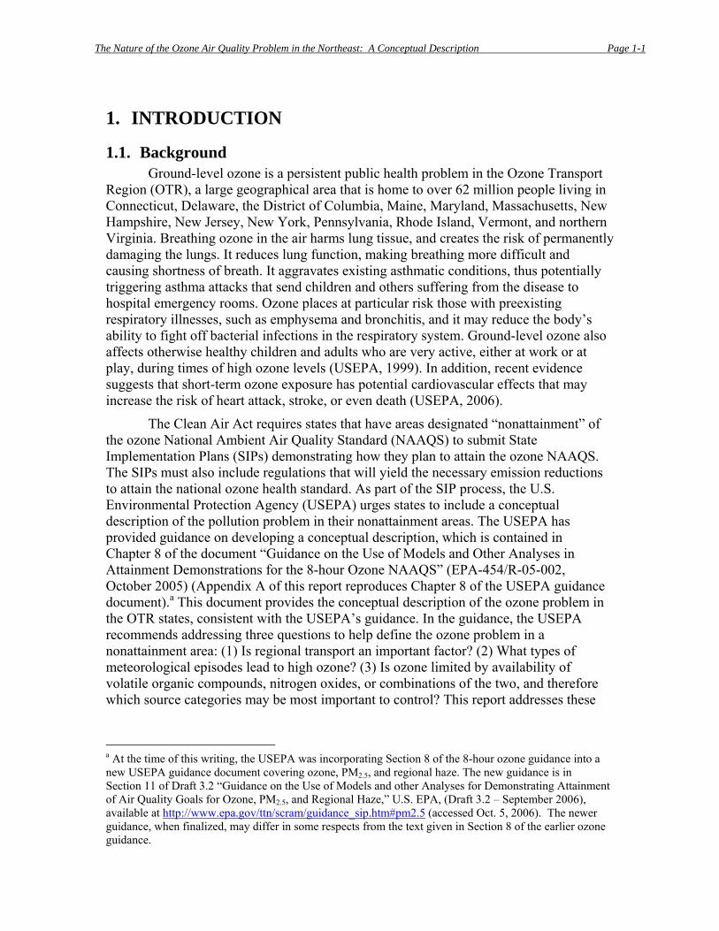
1.2. Ozone formation Ground-level ozone is formed in the atmosphere through a series of complex
chemical reactions involving sunlight, warm temperatures, nitrogen oxides (NOX) and volatile organic compounds (VOCs). Figure 1-1 is a conceptual picture of the emission sources and conditions contributing to ozone formation in the atmosphere. There are natural (biogenic) sources of NOX, such as formation by soil microbes, lightening, and forest fires, but the dominant NOX sources in the eastern United States arise from human activities, particularly the burning of fossil fuels in cars, trucks, power plants, and other combustion sources (MARAMA, 2005).
In contrast to NOX sources, there are significant biogenic sources of VOCs in the eastern United States that can play an important contributing role in ozone formation. Isoprene, a highly reactive natural VOC emitted typically by deciduous trees such as oak, is an important ozone precursor across large parts of the East. Isoprene emissions typically increase with temperature up to a point before high temperatures tend to shut off emissions as leaf stomata (pores) close to reduce water loss. The tendency for increasing isoprene emissions with increasing temperatures (up to a point) coincides with the temperature and sunlight conditions favorable for increased ozone production (MARAMA, 2005).
Human-caused (anthropogenic) VOC emissions are important and may dominate the VOC emissions by mass (weight) in an urban area, even though natural sources dominate in the overall region. Some anthropogenic VOCs, such as benzene, are toxic, and may increase risks of cancer or lead to other adverse health effects in addition to helping form ozone (MARAMA, 2005).
The Nature of the Ozone Air Quality Problem in the Northeast: A Conceptual Description Page 1-3
Figure 1-1. Conceptual picture of ozone formation in the atmosphere
Picture provided by the Maryland Department of the Environment.
The relationship between the relative importance of NOX and VOC emissions in producing ozone is complex. The relative ratio of NOX and VOC levels in the local atmosphere can affect the efficiency of local urban ozone production, and this can vary by time (hour or day) at the same urban location, as well as across locations within the same urban area. High NOX concentrations relative to VOC levels may hinder ozone production through the destruction of ozone by NOX (sometimes called “NOX scavenging”). The same NOX, however, when diluted relative to VOCs through the downwind transport and dispersal of a pollution plume, will promote ozone formation elsewhere.
1.3. Spatial pattern of ozone episodes in the OTR The day-to-day pattern of ground-level ozone varies according to meteorological
variables that include, but are not limited to, sunlight, air temperature, wind speed, and wind direction. Generally within the OTR, one would expect elevated ozone to occur more frequently in southernmost areas, where solar elevation angles are greater and cold frontal passages are fewer. A glance at monthly composite maps (for example, July-August 2002) at the USEPA AIRNOW website seems to confirm this (http://www.epa.gov/airnow/nemapselect.html). On some days, however, one notes that the highest ozone levels shift northward to mainly affect the northern part of the OTR. Other shifts are apparent between coastal and interior areas.
This variability of the daily ozone pattern is tied to variations in the atmosphere’s circulations over a range of scales, and how geographic features influence these
The Nature of the Ozone Air Quality Problem in the Northeast: A Conceptual Description Page 1-4
circulations. These features can include boundaries between land and sea, and the influence of the Appalachian Mountains on winds to their east over the Atlantic Coastal Plain.
For the OTR, Stoeckenius and Kemball-Cook (2005) have identified five general ozone patterns: (1) high ozone throughout the OTR; (2) high ozone confined to the extreme southeastern OTR; (3) high ozone along the I-95 corridor and northern New England; (4) high ozone in the western OTR; and (5) generally low ozone throughout the OTR. However, not all ozone episodes necessarily neatly fit into one of the five general patterns as daily conditions will vary and a given ozone episode may have characteristics that fall across several class types. These five general patterns, however, are a useful classification scheme for characterizing how representative an historical ozone episode is for possible use in air quality planning efforts. Appendix B presents the descriptions of the five general ozone patterns and their meteorological attributes as developed by Stoeckenius and Kemball-Cook (2005).
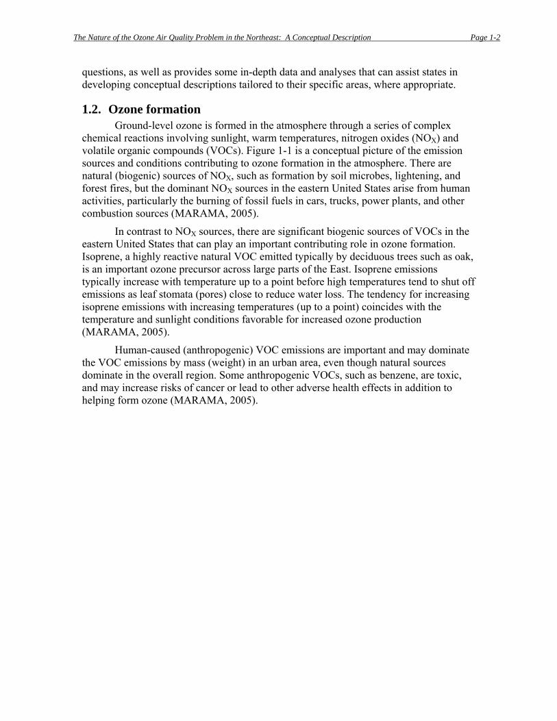
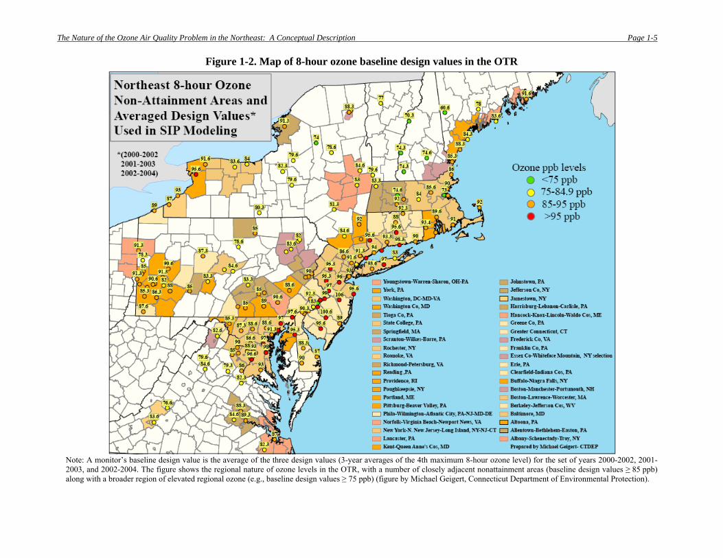
1.4. The regional extent of the ozone problem in the OTR Air monitoring demonstrates that areas with ozone problems in the OTR do not
exist in isolation. The map of Figure 1-2 shows an extensive pattern of closely adjacent ozone nonattainment in areas throughout the OTR. The 8-hour ozone baseline design values (defined in the figure caption) at the monitoring sites shown in the figure indicate extensive areas throughout the OTR with many monitors having values above the 8-hour ozone NAAQS of 0.08 ppm. In practice, this corresponds to levels equal to or greater than 0.085 ppm (equivalent to 85 ppb). The map also shows that many monitors outside the designated nonattainment areas of the OTR also record elevated ozone concentrations approaching the 8-hour ozone NAAQS (i.e., 75-84.9 ppb), even if not violating it. The many monitoring locations across that OTR measuring elevated ozone levels that approach or exceed the 8-hour ozone NAAQS give a strong indication of the regional nature of the OTR’s ozone problem.
The Nature of the Ozone Air Quality Problem in the Northeast: A Conceptual Description Page 1-5
Figure 1-2. Map of 8-hour ozone baseline design values in the OTR
Note: A monitor’s baseline design value is the average of the three design values (3-year averages of the 4th maximum 8-hour ozone level) for the set of years 2000-2002, 2001-2003, and 2002-2004. The figure shows the regional nature of ozone levels in the OTR, with a number of closely adjacent nonattainment areas (baseline design values ≥ 85 ppb) along with a broader region of elevated regional ozone (e.g., baseline design values ≥ 75 ppb) (figure by Michael Geigert, Connecticut Department of Environmental Protection).
The Nature of the Ozone Air Quality Problem in the Northeast: A Conceptual Description Page 1-6
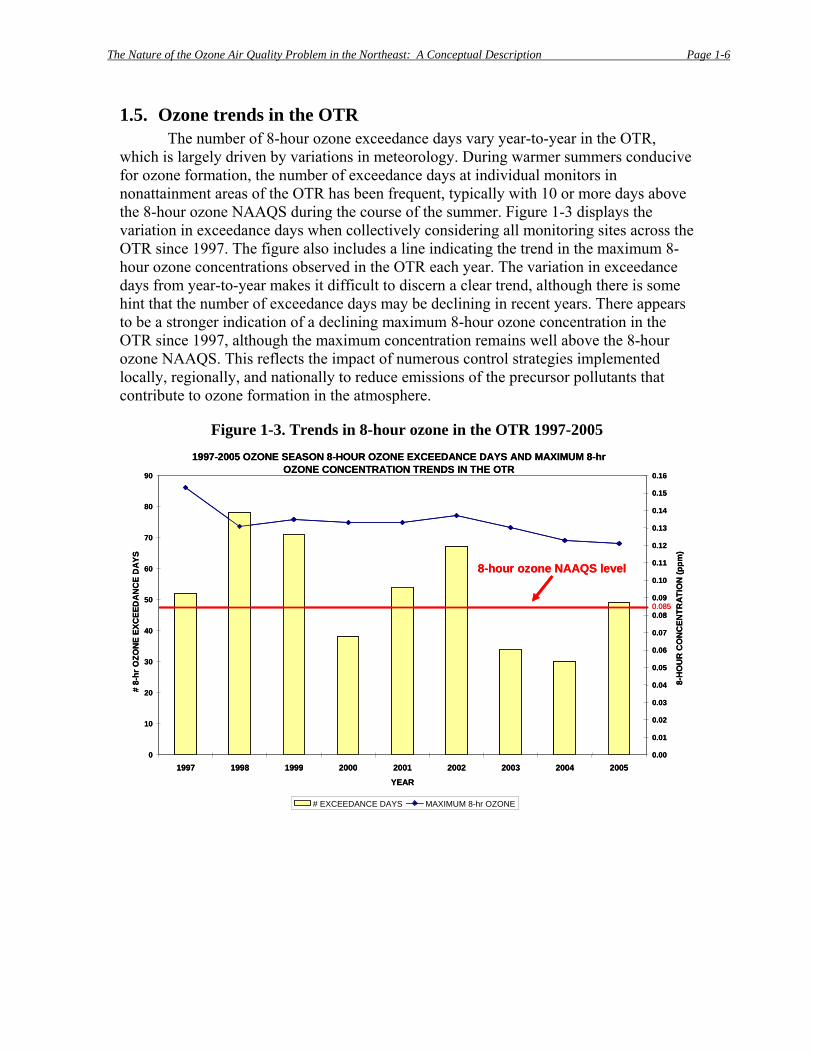
1.5. Ozone trends in the OTR The number of 8-hour ozone exceedance days vary year-to-year in the OTR,
which is largely driven by variations in meteorology. During warmer summers conducive for ozone formation, the number of exceedance days at individual monitors in nonattainment areas of the OTR has been frequent, typically with 10 or more days above the 8-hour ozone NAAQS during the course of the summer. Figure 1-3 displays the variation in exceedance days when collectively considering all monitoring sites across the OTR since 1997. The figure also includes a line indicating the trend in the maximum 8-hour ozone concentrations observed in the OTR each year. The variation in exceedance days from year-to-year makes it difficult to discern a clear trend, although there is some hint that the number of exceedance days may be declining in recent years. There appears to be a stronger indication of a declining maximum 8-hour ozone concentration in the OTR since 1997, although the maximum concentration remains well above the 8-hour ozone NAAQS. This reflects the impact of numerous control strategies implemented locally, regionally, and nationally to reduce emissions of the precursor pollutants that contribute to ozone formation in the atmosphere.
Figure 1-3. Trends in 8-hour ozone in the OTR 1997-2005
1997-2005 OZONE SEASON 8-HOUR OZONE EXCEEDANCE DAYS AND MAXIMUM 8-hr OZONE CONCENTRATION TRENDS IN THE OTR
0
10
20
30
40
50
60
70
80
90
1997 1998 1999 2000 2001 2002 2003 2004 2005
YEAR
# 8-
hr O
ZON
E EX
CEE
DA
NC
E D
AYS
0.00
0.01
0.02
0.03
0.04
0.05
0.06
0.07
0.08
0.09
0.10
0.11
0.12
0.13
0.14
0.15
0.16
8-H
OU
R C
ON
CEN
TRAT
ION
(ppm
)
# EXCEEDANCE DAYS MAXIMUM 8-hr OZONE
8-hour ozone NAAQS level
0.085
The Nature of the Ozone Air Quality Problem in the Northeast: A Conceptual Description Page 1-7
Note: The bars correspond to the number of 8-hour ozone exceedance days per year. The upper blue line indicates the trend in maximum 8-hour ozone concentrations in the OTR during 1997-2005. The lower red horizontal line indicates the level of the 8-hour ozone NAAQS (functionally 0.085 ppm). (Figure created by Tom Downs, Maine Dept. of Environmental Protection.)
The tables in Appendix C contain the frequency of ozone exceedance days for individual monitors in the OTR states from 1997 to 2005. Appendix D contains tables for the 8-hour ozone design values recorded at ozone monitors in the OTR during 1997-2005. These tables give an indication of the number of monitors in the OTR since 1997 that have exceeded the 8-hour NAAQS of 85 ppb (equal to 0.085 ppm in the tables of Appendix D) at some point in time.
1.6. History of ozone transport science
1.6.1. From the 1970s to the National Research Council report, 1991 Research studies conducted in the 1970s gave some of the earliest indications that
pollution transport plays an important role in contributing to air pollution problems in the OTR. An aircraft study in the summer of 1979 tracked a mass of ozone-laden air and its precursors leaving central Ohio, crossing the length of Pennsylvania, and entering the Northeast Corridor where it contributed upwards of 90 ppb to early morning ozone concentrations in the OTR prior to local ozone formation from local emissions (Clarke & Ching, 1983). Wolff and Lioy (1980) described a “river of ozone” extending from the Gulf Coast through the Midwest and into New England. A number of early studies also documented the role of large coal-fired power plants in forming significant amounts of ozone pollution that traveled far downwind from the power plant source and contributed to a large elevated background of regional ozone (Davis et al., 1974; Miller et al., 1978; Gillani & Wilson, 1980; Gillani et al., 1981; White et al., 1983). Section 2 below describes in more depth the observed meteorological processes identified as the ozone transport mechanisms important for the OTR.
On a regional scale, NOX emissions within areas of high VOC emissions, such as forested regions rich in isoprene, will produce elevated levels of ozone. A number of studies have now established that regional ozone formation over the eastern United States is limited primarily by the supply of anthropogenic NOX, with anthropogenic VOCs having less regional influence compared to their potential urban influence. This is due to the presence of significant amounts of natural VOCs across broad areas of the eastern United States (Trainer et al., 1987; Chameides et al., 1988; Sillman et al., 1990; McKeen et al., 1991; Chameides et al., 1992; Trainer et al., 1993; Jacob et al., 1993).
The presence of dispersed NOX emissions sources, such as coal-fired power plants, in rural regions rich in isoprene and other natural VOC emissions from trees and
The Nature of the Ozone Air Quality Problem in the Northeast: A Conceptual Description Page 1-8
other vegetation often leads to elevated regional ozone during the summer months. This ozone can then be transported into urban areas where it contributes to high background concentrations during the early morning hours before local production of ozone occurs from local precursor emissions (both NOX and VOCs).
In 1991, a National Research Council (NRC) committee, synthesizing the best available information at the time on ozone formation and transport in the eastern United States, reported (NRC, 1991):
High ozone episodes last from 3-4 days on average, occur as many as 7-10 times a year, and are of large spatial scale: >600,000 km2. Maximum values of non-urban ozone commonly exceed 90 ppb during these episodes, compared with average daily maximum values of 60 ppb in summer. An urban area need contribute an increment of only 30 ppb over the regional background during a high ozone episode to cause a violation of the National Ambient Air Quality Standard (NAAQS) in a downwind area. … Given the regional nature of the ozone problem in the eastern United States, a regional model is needed to develop control strategies for individual urban areas. [Note: The NRC discussion was in the context of the ozone NAAQS at the time of the NRC report, which was 0.12 ppm (120 ppb) averaged over one hour.] The observed ozone spatial scale of >600,000 km2 (>200,000 square miles) is
comparable to the combined size of Kentucky, Ohio, West Virginia, Pennsylvania, Maryland, New York, and New Jersey. Additional field studies and modeling efforts since the NRC report (described below) have reinforced its basic findings and provide a consistent and coherent body of evidence for transport throughout the eastern United States.
1.6.2. Ozone Transport Assessment Group (OTAG) 1995-1997 The increasing regulatory focus on broader regional approaches to ozone control
beyond the OTR began with the Ozone Transport Assessment Group (OTAG) in 1995. OTAG was a partnership between the USEPA, the Environmental Council of the States (ECOS), state and federal government officials, industry organizations, and environmental groups. OTAG’s goal was “to develop an assessment of and consensus agreement for strategies to reduce ground-level ozone and its precursors in the eastern United States” (OTAG, 1997a). The effort assessed transport of ground-level ozone across state boundaries in the 37-state OTAG region and developed a set of recommendations to the USEPA. OTAG completed its work in 1997.
OTAG supported a significant modeling effort of four regional ozone episodes across the eastern United States. OTAG’s Regional and Urban Scale Modeling Workgroup found that on a regional scale, modeled NOX reductions produced widespread ozone decreases across the eastern United States with limited ozone increases generally confined to some urban areas. Also on a regional scale, VOC reductions resulted in limited ozone decreases generally confined to urban areas (OTAG, 1997b).
The OTAG Air Quality Analysis Workgroup provided additional observational and other analytical results to inform model interpretation and the development of OTAG recommendations. Among its many finding, this Workgroup observed:
The Nature of the Ozone Air Quality Problem in the Northeast: A Conceptual Description Page 1-9
Low wind speeds (< 3 m/sec) enable the accumulation of ozone near local source areas. High winds (> 6 m/sec) reduce the concentrations but contribute to the long-range transport of ozone. The average range of ozone transport implied from an array of diverse methods is between 150 miles and 500 miles. However, the perceived range depends on whether one considers the average concentrations (300–500 miles) or peak concentrations (tens of miles at 120 ppb). The relative importance of ozone transport for the attainment of the new 80 ppb 8-hour standard is likely to be higher due to the closer proximity of nonattainment areas. (OTAG, 1997c) Based on the variety of technical work performed by multiple stakeholders during
the process, OTAG reached a number of major conclusions (OTAG, 1997d), including: • Regional NOX reductions are effective in producing ozone benefits; the more NOX reduced, the
greater the benefit. • Ozone benefits are greatest in the subregions where emissions reductions are made; the benefits
decrease with distance. • Both elevated (from tall stacks) and low-level NOX reductions are effective. • VOC controls are effective in reducing ozone locally and are most advantageous to urban
nonattainment areas. • Air quality data indicate that ozone is pervasive, that ozone is transported, and that ozone aloft is
carried over and transported from one day to the next.
The technical findings of OTAG workgroups were consistent with the modeling and observational studies of regional ozone in the eastern United States already appearing in the scientific literature at that time.
Through its work, OTAG engaged a broad group outside of the scientific community in the discussion of ozone transport. This brought a greater understanding of the role of ozone transport across the eastern United States that was then translated into air quality policy with the creation of a regional ozone control strategy focusing on the reduction of NOX emissions from power plants.
1.6.3. Northeast Oxidant and Particle Study (NE-OPS) 1998-2002 The Northeast Oxidant and Particle Study (NE-OPS) began in 1998 as a USEPA
sponsored project to study air quality issues in the Northeast. The study undertook four major field programs at a field site in northeastern Philadelphia during the summers of 1998, 1999, 2001, and 2002. It involved a collaborative effort among research groups from a number of universities, government laboratories, and representatives of the electric power industry in an investigation of the interplay between the meteorological and chemical processes that lead to air pollution events in the Northeast. A suite of measurement techniques at and above the earth’s surface gave a three-dimensional regional scale picture of the atmosphere. The studies found that horizontal transport aloft and vertical mixing to the surface are key factors in controlling the evolution and severity of air pollution episodes in the Northeast (Philbrick et al., 2003a).
At the conclusion of the 2002 summer field study, the NE-OPS researchers were able to draw several conclusions about air pollution episodes in Philadelphia and draw inferences from this to the conditions in the broader region. These include (Philbrick et al., 2003b):
• Transported air pollution from distant sources was a major contributor to all of the major summer air pollution episodes observed in the Philadelphia area.
• Regional scale meteorology is the major factor controlling the magnitude and timing of air pollution episodes.

The Nature of the Ozone Air Quality Problem in the Northeast: A Conceptual Description Page 1-10
• Knowledge of how the planetary boundary layer evolves over the course of a day is a critical input for modeling air pollutant concentrations because it establishes the mixing volume.
• Remote sensing and vertical profiling techniques are critical for understanding the processes governing air pollution episodes.
• Ground-based sensors do not detect high levels of ozone that are frequently trapped and transported in layers above the surface.
• Horizontal and vertical nighttime transport processes, such as the nocturnal low level jets and “dynamical bursting”b events, are frequent contributors of pollutants during the major episodes.
• Specific meteorological conditions are important in catalyzing the region for development of major air pollution episodes.
• Tethered balloon and lidar measurements suggest a very rapid down mixing of species from the residual boundary layer during the early morning hours that is too large to be accounted for on the basis of NOX reactions alone.
• Summer organic aerosols in Philadelphia consist of a relatively constant level of primary organic particulate matter, punctuated by extreme episodes with high levels of secondary organic aerosol during ozone events. Primary organic particulate matter is both biogenic and anthropogenic in nature, with the relative importance fluctuating from day to day, and possibly associated more strongly with northwest winds. Secondary aerosol formation events may be responsible for dramatic increases in particulate organic carbon, while the relatively constant contribution of primary sources could make a greater contribution to annual average particulate levels. More research is needed to sort out the relative contributions of anthropogenic and biogenic sources.
The findings on nocturnal low level jets occurring in concert with ozone pollution episodes are particularly salient for air quality planning for the OTR. In 19 of 21 cases where researchers observed nocturnal low level jets during the NE-OPS 2002 summer campaign in the Philadelphia area, they also saw peak 1-hour ozone levels exceeding 100 ppbv. The nocturnal low level jets were capable of transporting pollutants in air parcels over distances of 200 to 400 km. The field measurements indicating that these jets often occur during periods of large scale stagnation in the region demonstrate the important role nocturnal low level jets can play in effectively transporting air pollutants during air pollution episodes (Philbrick et al., 2003b).
The upper air observations using tethered balloons and lidar indicated the presence of high pollutant concentrations trapped in a residual layer above the surface, thus preserving the pollutants from destruction closer to the surface. Ozone, for example, when trapped in an upper layer during nighttime hours is not subject to destruction by NOX scavenging from low-level emission sources (i.e., cars and trucks) or deposition to surfaces like vegetation, hence it is available for horizontal transport by nocturnal low level jets. The following day, it can vertically transport back down to the surface through “bursting events” and daytime convection. When involving an upper layer of ozone-laden air horizontally transported overnight by a nocturnal low level jet, downward mixing can increase surface ozone concentrations in the morning that is not the result of local ozone production (Philbrick et al., 2003b).
1.6.4. NARSTO 2000 NARSTO (formerly known as the North American Research Strategy for
Tropospheric Ozone) produced “An Assessment of Tropospheric Ozone Pollution – A
b “Dynamical bursting” events occur in the early morning hours due to instabilities in the lower atmosphere caused by differences in wind speeds at different altitudes below the layer of maximum winds. Bursting events can vertically mix air downwards to the surface (see Philbrick et al., 2003b at p. 36).
The Nature of the Ozone Air Quality Problem in the Northeast: A Conceptual Description Page 1-11
North American Perspective” in 2000 to provide a policy-relevant research assessment of ozone issues in North America (NARSTO, 2000). While the NARSTO Assessment is continental in scope, it encompasses issues relevant to the OTR, including results from a NARSTO-Northeast (NARSTO-NE) field campaign.
Several policy-relevant findings from the NARSTO Assessment are of relevance to the OTR (NARSTO, 2000):
• Available information indicates that ozone accumulation is strongly influenced by extended periods of limited mixing, recirculation of polluted air between the ground and aloft, and the long-range transport of ozone and its precursors. As a result, air quality management strategies require accounting for emissions from distant as well as local sources.
• Local VOC emission reductions may be effective in reducing ozone in urban centers, while NOX emission reductions become more effective at distances removed from urban centers and other major precursor emissions.
• The presence of biogenic emissions complicates the management of controllable precursor emissions and influences the relative importance of VOC and NOX controls.
• The effectiveness of VOC and NOX control strategies is not uniquely defined by the location or nature of emissions. It is now recognized that the relative effectiveness of VOC and NOX controls may change from one location to another and even from episode to episode at the same location.
The NARSTO Assessment identified the stagnation of synoptic scale (>1000 km2) high pressure systems as a commonly occurring weather event leading to ozone pollution episodes. These systems are warm air masses associated with weak winds, subsiding air from above, and strong inversions capping the planetary boundary level in the central region of the high. The warm air mass can settle into place for days to more than a week, and in the eastern U.S. tend to slowly track from west to east during the summer. These conditions result in the build up of pollution from local sources with reduced dispersion out of the region. In terms of air quality, the overall appearance of such systems is the presence of numerous local or urban-scale ozone pollution episodes embedded within a broader regional background of elevated ozone concentrations (NARSTO, 2000 at p. 3-34).
While stagnation implies little movement, the NARSTO Assessment found that a variety of processes can lead to long-range transport of air pollutants that initially accumulated in these large-scale stagnation events. Over time, pollution plumes meander, merge, and circulate within the high pressure system. Because of the difference in pressures, pollutant plumes that eventually migrate to the edges of a high pressure system get caught in increasing winds at the edge regions, creating more homogeneous regional pollution patterns. Stronger winds aloft capture the regional pollutant load, and can transport it for hundreds of kilometers downwind of the stagnated air mass’s center (NARSTO, 2000 at p. 3-34). For example, air flow from west to east over the Appalachian Mountains can move air pollution originating within the Ohio River Valley into the OTR.
Studies undertaken by the NARSTO-NE field program also observed several regional scale meteorological features arising from geographical features in the eastern U.S. that affect pollutant transport. One important feature is the channeled flow of a nocturnal low level jet moving air pollution from the southwest to the northeast along the Northeast Corridor during overnight hours. The NARSTO-NE field program observed
The Nature of the Ozone Air Quality Problem in the Northeast: A Conceptual Description Page 1-12
nocturnal low level jets on most nights preceding regional ozone episodes in the OTR, consistent with the observations of the NE-OPS campaign.
Another important smaller scale transport mechanism is the coastal sea breeze that can sweep ashore pollutants originally transported over the ocean parallel to the coastline. An example of this is the high ozone levels seen at times along coastal Maine that move in from the Gulf of Maine after having been transported in pollution plumes from Boston, New York City, and other Northeast Corridor locations (NARSTO, 2000 at pp. 3-34 through 3-37).
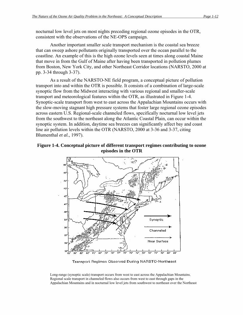
As a result of the NARSTO-NE field program, a conceptual picture of pollution transport into and within the OTR is possible. It consists of a combination of large-scale synoptic flow from the Midwest interacting with various regional and smaller-scale transport and meteorological features within the OTR, as illustrated in Figure 1-4. Synoptic-scale transport from west to east across the Appalachian Mountains occurs with the slow-moving stagnant high pressure systems that foster large regional ozone episodes across eastern U.S. Regional-scale channeled flows, specifically nocturnal low level jets from the southwest to the northeast along the Atlantic Coastal Plain, can occur within the synoptic system. In addition, daytime sea breezes can significantly affect bay and coast line air pollution levels within the OTR (NARSTO, 2000 at 3-36 and 3-37, citing Blumenthal et al., 1997).
Figure 1-4. Conceptual picture of different transport regimes contributing to ozone episodes in the OTR
Long-range (synoptic scale) transport occurs from west to east across the Appalachian Mountains. Regional scale transport in channeled flows also occurs from west to east through gaps in the Appalachian Mountains and in nocturnal low level jets from southwest to northeast over the Northeast
The Nature of the Ozone Air Quality Problem in the Northeast: A Conceptual Description Page 1-13
Corridor. Daytime sea breezes can affect local coastal areas by bringing in air pollution originally transported near the surface across water parallel to the coast (e.g., along the Maine coastline). Figure from NARSTO, 2000, citing Blumenthal et al., 1997.
1.6.5. New England Air Quality Study (NEAQS) 2002-2004 The New England Air Quality Study (NEAQS) has to date conducted field
campaigns during the summers of 2002 and 2004 to investigate air quality on the Eastern Seaboard and transport of North American emissions into the North Atlantic (NEAQS, 2002). Transport of air pollution into the Gulf of Maine and subsequently into coastal areas of northern New England received extensive attention.
High ozone levels in northern New England occur with light to moderate winds from source regions in the Northeast urban corridor, rather than under locally stagnant conditions. The most important transport pathways leading to high ozone in coastal New Hampshire and Maine are over water rather than over land. Transport over water is particularly important in this northern region of the OTR for several reasons. First, there is a persistent pool of cooler water in the northern and eastern Gulf of Maine and Bay of Fundy. This creates a smoother transport surface for air pollutants relative to land transport, with a decrease in convective (vertical) mixing. Second, deposition of pollutants to the water surface is very small compared to the more rapid deposition occurring on land. Third, the lack of convective mixing allows pollution to be transported in different directions in layers at different heights in the atmosphere (Angevine et al., 2004).
During the summer of 2002, researchers observed two transport events into coastal northern New England. The first occurring on July 22 through July 23 involved large-scale synoptic transport in a 400-600 m layer over the Gulf of Maine that was in contact with the water’s surface. The southwesterly flow brought ozone pollution up from the New York City, Boston and other northeastern urban locations into coastal northern New England. Ozone monitors on Maine’s coast extending from the New Hampshire border to Acadia National Park recorded elevated 1-hour average ozone levels between 88 and 120 ppb during this period. In a later episode during August 11-14, ozone and wind observations indicated the role of local-scale transport via a sea breeze (southeasterly flow) bringing higher ozone levels into coastal New Hampshire from a polluted layer originally transported off shore in the Gulf of Maine in a southwesterly flow arising out of the Northeast urban corridor. Transport in an elevated layer also occurred with higher ozone recorded at a monitor on Cadillac Mountain in Acadia National Park relative to two monitors located at lower elevations in the park (Angevine et al., 2004).
The results of NEAQS indicate the important conditions contributing to ozone transport along the northern New England coast. The cool waters of the Gulf of Maine allow for transport of air pollutants over distances of 20-200 km in stable layers at the water’s surface with little pollutant deposition or dilution. Sea breezes can modify large-scale synoptic transport over the ocean and bring high ozone levels into particular sites located on the coast. Transport within higher layers above the Gulf of Maine can carry pollutants over much greater distances, 200-2000 km (Angevine et al., 2004).

The Nature of the Ozone Air Quality Problem in the Northeast: A Conceptual Description Page 1-14
1.6.6. Regional Atmospheric Measurement, Modeling, and Prediction Program (RAMMPP) 2003
The Regional Atmospheric Measurement, Modeling, and Prediction Program (RAMMPP) is a program led by researchers at the University of Maryland. Its focus is developing a state-of-the-art scientific research tool to improve understanding of air quality in the mid-Atlantic region of the United States. It has a number of facets, including ozone and PM2.5 pollutant level forecasting, aircraft, and surface measurements, real-time weather forecasting, and chemical transport modeling.
During the August 2003 electrical blackout in the eastern United States, one of the largest in North American history, scientists with RAMMPP were able to obtain airborne measurements that directly recorded changes in air pollution due to the virtual shutdown of numerous coal-fired power plants across a large part of this region (Marufu et al., 2004). Initially, aircraft measurements were collected early in the day on August 15, 2003 above western Maryland, which was outside the blackout region. These measurements were compared with aircraft measurements taken later that day over central Pennsylvania, about 24 hours into the blackout. The comparison indicated a decrease in ozone concentrations of ~50 percent within the blackout region (as well as >90 percent decrease in SO2 and ~70 percent reduction in light scattered by particles). These reductions were also consistent with comparisons to measurements obtained over central Pennsylvania the previous year during a period of similar synoptic patterns as occurred during the blackout. Forward trajectories indicated that the decrease in air pollution during the blackout benefited much of the eastern United States. The decrease in ozone was greater than expected based on estimates of the relative contribution of power plant NOX emissions to ozone formation in the region. The researchers suggested that this could be due to underestimation of power plant emissions, poor representation of power plant plumes in emission models, or an incomplete set of atmospheric chemical reactions in photochemical models. This accidental “real world” experiment indicates that ozone formation across a large part of the eastern United States is sensitive to power plant NOX emissions, and may be even more sensitive to NOX reductions from these sources than currently predicted by air quality modeling.
1.7. Summary The chemistry of ozone formation in the atmosphere involves reactions of NOX
and VOC emissions from numerous sources during periods of warm temperatures and abundant sunshine. The day-to-day pattern of ground-level ozone in the OTR varies according to a number of meteorological variables, such as sunlight, temperature, wind speed, and wind direction. High levels of ozone within the OTR do not occur in isolation, indicating a broad regional air quality problem. Trends in 8-hour ozone levels since 1997 indicate improvement in air quality, a reflection of numerous control strategies implemented locally, regionally, and nationally to reduce emissions of the pollutants that contribute to ozone formation.
The scientific literature prior to 1985 contains a number of peer reviewed papers describing observed episodes of ozone and precursor pollutant transport. In 1991, a National Research Council report summarized the state-of-the-science, which further highlighted the broad regional nature of the ozone problem in the eastern U.S. Since then,

The Nature of the Ozone Air Quality Problem in the Northeast: A Conceptual Description Page 1-15
multiple collaborative efforts and field campaigns have further investigated specific aspects of the regional ozone problem affecting the OTR, and these provide a significant foundational basis for informed policy decisions to improve air quality.
The Nature of the Ozone Air Quality Problem in the Northeast: A Conceptual Description Page 1-16
References Angevine, W.M., C.J. Senff, A.B. White, E.J. Williams, J. Koermer, S.T.K. Miller, R. Talbot, P.E. Johnston, S.A. McKeen, and T. Downs. “Coastal boundary layer influence on pollutant transport in New England.” J. Applied Meteor. 43, 1425-1437, 2004. Blumenthal, D.L., F. Lurmann, N. Kumar., T. Dye, S. Ray, M. Korc, R. Londergan, and G. Moore. Transport and mixing phenomena related to ozone exceedances in the northeast U.S. EPRI Report TR-109523, Electric Power Research Institute, Palo Alto, CA, 1997. Chameides, W.L., R.W. Lindsay, J. Richardson, and C.S. Kiang. “The role of biogenic hydrocarbons in urban photochemical smog: Atlanta as a case study.” Science 241, 1473-1475, 1988. Chameides, W.L., F. Fehsenfeld, M.O. Rodgers, C. Cardelino, J. Martinez, D. Parrish, W. Lonneman, D.R. Lawson, R.A. Rasmussen, P. Zimmerman, J. Greenberg, P. Middleton, and T. Wang. “Ozone precursor relationships in the ambient atmosphere.” J. Geophys. Res. 97, 6037-6055, 1992. Clarke, J.F., and J.K.S. Ching. “Aircraft observations of regional transport of ozone in the northeastern United States.” Atmos. Envt. 17, 1703-1712, 1983. Davis, D.D., G. Smith, and G. Klauber. “Trace gas analysis of power plant plumes via aircraft measurement: O3, NOX, and SO2 chemistry.” Science 186, 733-736, 1974. Gillani, N.V., and W.E. Wilson. “Formation and transport of ozone and aerosols in power plant plumes.” Annals N.Y. Acad. Sciences 338, 276-296, 1980. Gillani, N.V., S. Kohli, and W.E. Wilson. “Gas-to-particle conversion of sulfur in power plant plumes – I. Parameterization of the conversion rate for dry, moderately polluted ambient conditions.” Atmos. Envt. 15, 2293-2313, 1981. Jacob, D.J., J.A. Logan, G.M. Gardner, R.M. Yevich, C.M. Spivakovsky, S.C. Wofsy, S. Sillman, and M.J. Prather. “Factors regulating ozone over the United States and its export to the global atmosphere.” J. Geophys. Res. 98, 14,817-14,826, 1993. MARAMA (Mid-Atlantic Regional Air Management Association). A guide to mid-Atlantic regional air quality. MARAMA. Baltimore, MD, pp. 2-3, 2005 (available on-line at www.marama.org/reports). Marufu, L.T., B.F. Taubman, B. Bloomer, C.A. Piety, B.C. Doddridge, J.W. Stehr, and R.R. Dickerson. “The 2003 North American electrical blackout: An accidental experiment in atmospheric chemistry.” Geophys. Res. Lett. 31, L13106, doi:10.1029/2004GL019771, 2004.
The Nature of the Ozone Air Quality Problem in the Northeast: A Conceptual Description Page 1-17
McKeen, S.A., E.-Y. Hsie, and S.C. Liu. “A study of the dependence of rural ozone on ozone precursors in the eastern United States.” J. Geophys. Res. 96, 15,377-15,394, 1991. Miller, D.F., A.J. Alkezweeny, J.M. Hales, and R.N. Lee. “Ozone formation related to power plant emissions.” Science 202, 1186-1188, 1978 NARSTO. An Assessment of Tropospheric Ozone Pollution. NARSTO, July 2000. NEAQS (New England Air Quality Study) 2002, http://www.al.noaa.gov/NEAQS/ (accessed June 20, 2006). NRC (National Research Council). Rethinking the ozone problem in urban and regional air pollution. National Academy Press. Washington, DC, pp. 105-106, 1991. OTAG (Ozone Transport Assessment Group). OTAG Technical Supporting Document, Appendix K – Summary of Ozone Transport Assessment Group recommendations to the U.S. Environmental Protection Agency as of June 20, 1997a. Available at http://www.epa.gov/ttn/naaqs/ozone/rto/otag/finalrpt/chp1/toc.htm. OTAG (Ozone Transport Assessment Group). OTAG Technical Supporting Document. Chapter 2 – Regional and Urban Scale Modeling Workgroup. 1997b. Available at http://www.epa.gov/ttn/naaqs/ozone/rto/otag/finalrpt/chp2_new/toc.htm. OTAG (Ozone Transport Assessment Group). OTAG Technical Supporting Document. Chapter 4 – Air Quality Analysis Workgroup. 1997c. Available at http://www.epa.gov/ttn/naaqs/ozone/rto/otag/finalrpt/chp4/toc.htm. OTAG (Ozone Transport Assessment Group). OTAG Technical Supporting Document. Chapter 1 – Overview. 1997d. Available at http://www.epa.gov/ttn/naaqs/ozone/rto/otag/finalrpt/. Philbrick, C.R., W.F. Ryan, R.D. Clark, B.G. Doddridge, P. Hopke, and S.R. McDow. “Advances in understanding urban air pollution from the NARSTO-NEOPS program.” 83rd American Meteorological Society 5th Conference on Atmospheric Chemistry, Long Beach, CA, Feb. 8-12, 2003a. Philbrick, C.S., W. Ryan, R. Clark, P. Hopke, and S. McDow. Processes controlling urban air pollution in the Northeast: Summer 2002. Final Report for the Pennsylvania Department of Environmental Protection, July 25, 2003b. Available at http://lidar1.ee.psu.edu/neopsWeb/publicSite/neopsdep/Final%20Rep-Part%201-7.pdf. Sillman, S., J.A. Logan, and S.C. Wofsy. “The sensitivity of ozone to nitrogen oxides and hydrocarbons in regional ozone episodes.” J. Geophys. Res. 95, 1837-1851, 1990.
The Nature of the Ozone Air Quality Problem in the Northeast: A Conceptual Description Page 1-18
Stoeckenius, T. and Kemball-Cook, S. “Determination of representativeness of 2002 ozone season for ozone transport region SIP modeling.” Final Report prepared for the Ozone Transport Commission, 2005. Trainer, M., E.J. Williams, D.D. Parrish, M.P. Buhr, E.J. Allwine, H.H. Westberg, F.C. Fehsenfeld, and S.C. Liu. “Models and observations of the impact of natural hydrocarbons on rural ozone.” Nature 329, 705-707, 1987. Trainer, M., D.D. Parrish, M.P. Buhr, R.B. Norton, F.C. Fehsenfeld, K.G. Anlauf, J.W. Bottenheim, Y.Z. Tang, H.A. Wiebe, J.M. Roberts, R.L. Tanner, L. Newman, V.C. Bowersox, J.F. Meagher, K.J. Olszyna, M.O. Rodgers, T. Wang, H. Berresheim, K.L. Demerjian, and U.K. Roychowdhury. “Correlation of ozone with NOy in photochemically aged air.” J. Geophys. Res. 98, 2917-2925, 1993. USEPA. Ozone and your Health, EPA-452/F-99-003, September 1999 (available at http://www.airnow.gov/index.cfm?action=static.brochure). USEPA. Technical Support Document for the Final Clean Air Interstate Rule: Air Quality Modeling. USEPA OAQPS, March 2005. Available at http://www.epa.gov/cleanairinterstaterule/pdfs/finaltech02.pdf. USEPA. Air Quality Criteria for Ozone and Related Photochemical Oxidants: Volume 1. USEPA, EPA-600/R-05/004aF, February 2006. White, W.H., D.E. Patterson, and W.E. Wilson, Jr. “Urban exports to the nonurban troposphere: Results from Project MISTT.” J. Geophys. Res. 88, 10,745-10,752, 1983. Wolff, G.T., and P.J. Lioy. “Development of an ozone river associated with synoptic scale episodes in the eastern United States.” Envtl. Sci. & Technol. 14, 1257-1260, 1980.
The Nature of the Ozone Air Quality Problem in the Northeast: A Conceptual Description Page 2-1
2. METEOROLOGY AND EVOLUTION OF OZONE EPISODES IN THE OZONE TRANSPORT REGION
The following sections describe current knowledge of the factors contributing to ozone episodes in the OTR. The general description of weather patterns comes mainly from the work of Ryan and Dickerson (2000) done for the Maryland Department of the Environment. Further information is drawn from work by Hudson (2005) done for the Ozone Transport Commission and from a mid-Atlantic regional air quality guide by MARAMA (2005). The regional nature of the observed ozone episodes in the OTR is reinforced in modeling studies by the USEPA for the Clean Air Interstate Rule.
2.1. Large-scale weather patterns Ryan and Dickerson (2000) have described the general meteorological features
conducive to ozone formation and transport that are pertinent to the OTR. On the local scale, meteorological factors on which ozone concentrations depend are the amount of available sunlight (ultraviolet range), temperature, and the amount of space (volume) in which precursor emissions mix. Sunlight drives the key photochemical reactions for ozone and its key precursors and the emissions rates of many precursors (isoprene for example) are temperature dependent. Emissions confined within a smaller volume result in higher concentrations of ozone. Winds in the lowest 2 km of the atmosphere cause horizontal mixing while vertical temperature and moisture profiles drive vertical mixing. High ozone is typically associated with weather conditions of few clouds, strong temperature inversions, and light winds.
The large-scale weather pattern that combines meteorological factors conducive to high ozone is the presence of a region of upper air high pressure (an upper air ridge) with its central axis located west of the OTR. The OTR east of the axis of the high-pressure ridge is characterized by subsiding (downward moving) air. This reduces upward motion necessary for cloud formation, increases temperature, and supports a stronger lower level inversion. While the upper air ridge is located west of the OTR, surface high pressure is typically quite diffuse across the region. This pattern occurs throughout the year but is most common and longer lived in the summer months (Ryan and Dickerson, 2000).
The large, or synoptic, scale, weather pattern sketched above has important implications for transport into and within the OTR. First, the persistence of an upper air ridge west of the OTR drives generally west to northwest winds that can carry ozone generated outside the OTR into the OTR. A key point from this wind-driven transport mode is that stagnant air is not always a factor for high ozone episodes in the OTR. Second, the region in the vicinity of the ridge axis, being generally cloud free, will experience significant radiational cooling after sunset and therefore a strong nocturnal inversion will form. This inversion, typically only a few hundred meters deep, prevents ozone and its precursors from mixing downward overnight. Above the inversion layer, there is no opportunity for destruction of the pollutants by surface deposition, thus increasing the pollutants’ lifetimes aloft and consequently their transport distances. Third, with diffuse surface high pressure, smaller scale effects can become dominant in the
The Nature of the Ozone Air Quality Problem in the Northeast: A Conceptual Description Page 2-2
lowest layers of the atmosphere. These include bay and land breezes, the Appalachian lee side trough, and the development of the nocturnal low level jet. Nocturnal low-level jets are commonly observed during high ozone events in the OTR (Ryan and Dickerson, 2000).
As previously mentioned in Section 1, Stoeckenius and Kemball-Cook (2005) have identified five ozone patterns in the OTR as a guide to an historical ozone episode’s representativeness for air quality planning purposes. They also described the meteorological conditions that are generally associated with each of these patterns. Appendix B presents the five types with the additional meteorological detail.
2.2. Meteorological mixing processes An important element in the production of severe ozone events is the ability of the
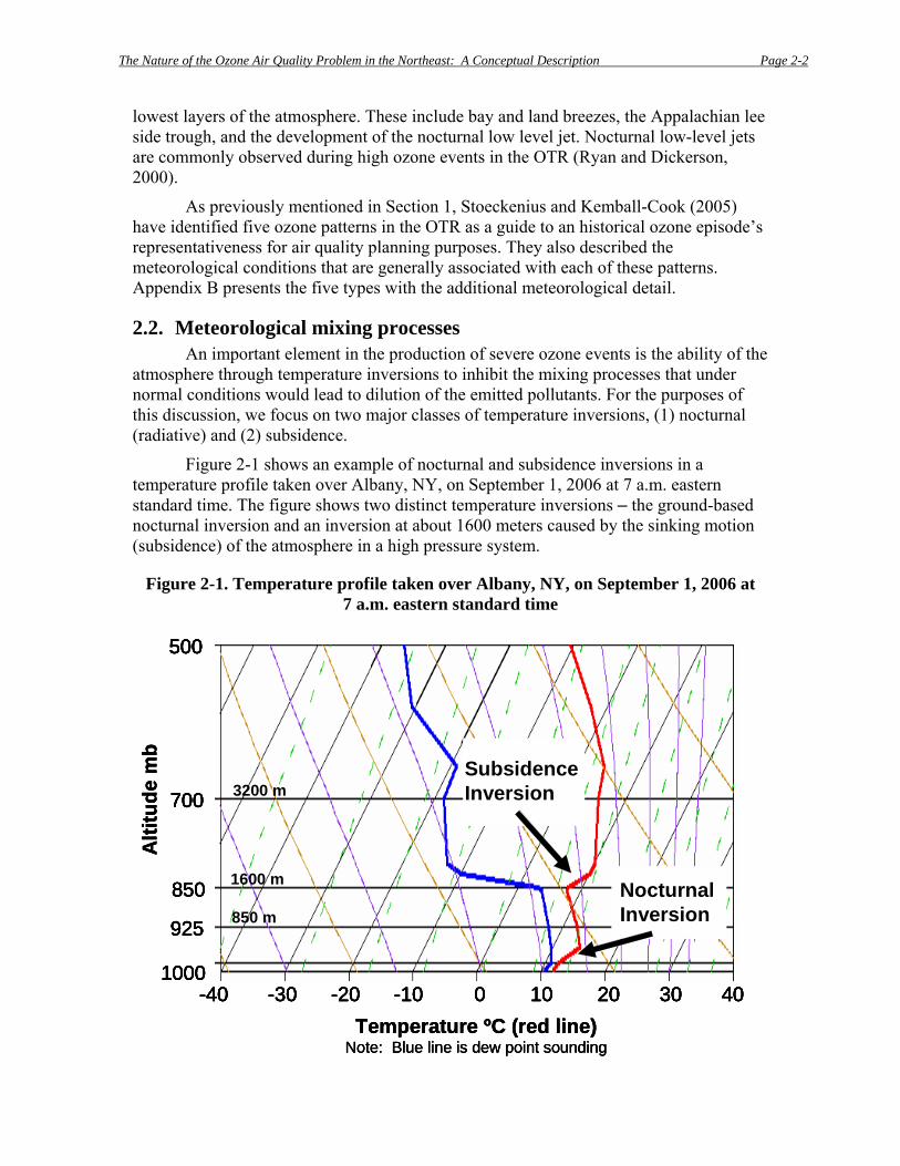
atmosphere through temperature inversions to inhibit the mixing processes that under normal conditions would lead to dilution of the emitted pollutants. For the purposes of this discussion, we focus on two major classes of temperature inversions, (1) nocturnal (radiative) and (2) subsidence.
Figure 2-1 shows an example of nocturnal and subsidence inversions in a temperature profile taken over Albany, NY, on September 1, 2006 at 7 a.m. eastern standard time. The figure shows two distinct temperature inversions – the ground-based nocturnal inversion and an inversion at about 1600 meters caused by the sinking motion (subsidence) of the atmosphere in a high pressure system.
Figure 2-1. Temperature profile taken over Albany, NY, on September 1, 2006 at 7 a.m. eastern standard time
-40 -30 -20 -10 0 10 20 30 40
1000
925
850
700
500
SubsidenceInversion
NocturnalInversion
Temperature ºC (red line)Note: Blue line is dew point sounding
Alti
tude
mb
1600 m
3200 m
850 m
-40 -30 -20 -10 0 10 20 30 401000
925
850
700
500
SubsidenceInversion
NocturnalInversion
Temperature ºC (red line)Note: Blue line is dew point sounding
Alti
tude
mb
-40 -30 -20 -10 0 10 20 30 401000
925
850
700
500
SubsidenceInversion
NocturnalInversion
-40 -30 -20 -10 0 10 20 30 401000
925
850
700
500
-40 -30 -20 -10 0 10 20 30 401000
925
850
700
500
SubsidenceInversionSubsidenceInversion
NocturnalInversionNocturnalInversion
Temperature ºC (red line)Note: Blue line is dew point sounding
Alti
tude
mb
1600 m
3200 m
850 m
The Nature of the Ozone Air Quality Problem in the Northeast: A Conceptual Description Page 2-3
2.2.1. Nocturnal inversions Land surfaces are far more efficient at radiating heat than the atmosphere above,
hence at night, the Earth’s surface cools more rapidly than the air. That temperature drop is then conveyed to the lowest hundred meters of the atmosphere. The air above this layer cools more slowly, and a temperature inversion forms. The inversion divides the atmosphere into two layers that do not mix. Below the nocturnal surface inversion, the surface winds are weak and any pollutants emitted overnight accumulate. Above the inversion, winds continue through the night and can even become stronger as the inversion isolates the winds from the friction of the rough surface.
In the morning, the sun warms the Earth’s surface, and conduction and convection transfer heat upward to warm the air near the surface. By about 10:00 – 11:00 a.m., the temperature of the surface has risen sufficiently to remove the inversion. Air from above and below the inversion can then mix freely. Depending on whether the air above the inversion is cleaner or more polluted than the air at the surface, this mixing can either lower or increase air pollution levels.
2.2.2. Subsidence inversions Severe ozone events are usually associated with high pressure systems. In the
upper atmosphere, the winds around a high pressure system move in a clockwise direction. At the ground, friction between the ground and the winds turns the winds away from the center of the system and “divergence” occurs, meaning that air at the surface moves away from the center. With the movement of air horizontally away from the center of the high at the surface, air aloft moves vertically downward (or “subsides”) to replace the air that left. Thus, the divergence away from the high pressure system gives rise to subsidence of the atmosphere above the high. The subsiding motion causes the air to warm as it moves downward and is compressed. As the warmer air meets the colder air below, it forms an inversion. A subsidence inversion is particularly strong because it is associated with this large scale downward motion of the atmosphere. The subsidence inversion caps pollution at a higher altitude in the atmosphere (typically from 1200 to 2000 meters), and it is far more difficult to break down than the nocturnal inversion. Hence the subsidence inversion limits vertical mixing in the middle of the day during an air pollution episode, keeping pollutants trapped closer to the ground.
2.3. Meteorological transport processes
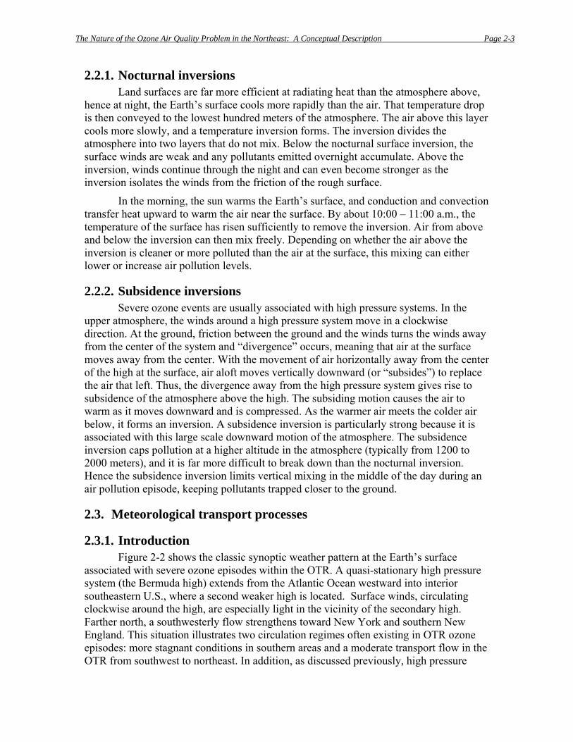
2.3.1. Introduction Figure 2-2 shows the classic synoptic weather pattern at the Earth’s surface
associated with severe ozone episodes within the OTR. A quasi-stationary high pressure system (the Bermuda high) extends from the Atlantic Ocean westward into interior southeastern U.S., where a second weaker high is located. Surface winds, circulating clockwise around the high, are especially light in the vicinity of the secondary high. Farther north, a southwesterly flow strengthens toward New York and southern New England. This situation illustrates two circulation regimes often existing in OTR ozone episodes: more stagnant conditions in southern areas and a moderate transport flow in the OTR from southwest to northeast. In addition, as discussed previously, high pressure
The Nature of the Ozone Air Quality Problem in the Northeast: A Conceptual Description Page 2-4
systems exhibit subsidence, which results in temperature inversions aloft, and cloud free skies.
Closer to the surface, the Appalachian Mountains induce changes in the wind field that also play important roles in the formation and transport of ozone in the OTR. The mountains act as a physical barrier confining, to some degree, pollution to the coastal plain. They also induce local effects such as mountain and valley breezes, which, in the case of down-slope winds, can raise surface temperatures thereby increasing chemical reactivity. In addition, mountains create a lee side trough, which helps to channel a more concentrated ozone plume, and contribute to the formation of nocturnal low level jets, the engine of rapid nighttime transport.
The Atlantic Ocean also plays a strong role during ozone episodes where sea breezes can draw either heavily ozone-laden or clean marine air into coastal areas.
Figure 2-2. Schematic of a typical weather pattern associated with severe ozone episodes in the OTR
Meteorological processes that transport ozone and its precursors into and within the OTR can roughly be broken down into three levels: ground, mid and upper. The following sections discuss the three wind levels associated with meteorological transport processes in more detail.
The Nature of the Ozone Air Quality Problem in the Northeast: A Conceptual Description Page 2-5
2.3.2. Ground level winds
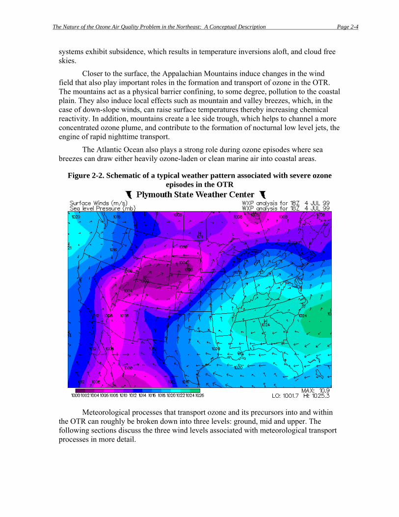
Land, sea, mountain, and valley breezes In the OTR, land and sea breezes, and mountain and valley breezes can have an
important influence on local air quality. These local winds are driven by a difference in temperature that produces a difference in pressure. Figure 2-3 shows a schematic of the formation of a sea breeze. The sea breeze forms in the afternoon when the land is considerably hotter than the ocean or bay. Air then flows from the high pressure over the ocean toward the low pressure over land. At night, the opposite may happen as the land cools to below the ocean’s temperature, and a land breeze blows out to sea. Because the nighttime land and water temperature differences are usually much smaller than in the day, the land breeze is weaker than the sea breeze. Sea breezes typically only penetrate a few kilometers inland because they are driven by temperature contrasts that disappear inland.
Figure 2-3. Illustration of a sea breeze and a land breeze
a) Sea Breeze b) Land Breeze Figure from Lutgens & Tarbuck, 2001.
Along coastlines, such as coastal New England, sea breezes bring in air pollution transported near the surface over water from urban locations located to the southwest. Figure 2-4 shows the average 2000-2002 wind direction frequency for elevated 1-hour ozone in the vicinity of the Kennebec and Penobscot Rivers in Maine. There is a clear maximum of pollution in the direction of the sea breeze. These sites are located many miles upriver from the coast, and receive ozone transported over water from the sea up through the coastal bays and rivers.
In other cases, sea breezes can affect air quality in coastal cities because, under stagnant synoptic-scale winds, a city’s emissions may be recirculated or pushed back over land after having drifted out over the sea earlier. Before sea breeze circulation begins, air pollution from a coastal city can move out over the water. In the absence of a shift in winds due to a sea breeze, the city’s air pollution will be blown away. When a sea breeze circulation sets up, however, the polluted air is pushed back toward the city. The sea breeze only pushes a few miles inland, which is where the barrier to mixing lies. Later in the day, the air may be quite clean on the ocean side of the city, but the air is
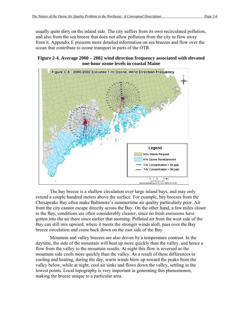
The Nature of the Ozone Air Quality Problem in the Northeast: A Conceptual Description Page 2-6
usually quite dirty on the inland side. The city suffers from its own recirculated pollution, and also from the sea breeze that does not allow pollution from the city to flow away from it. Appendix E presents more detailed information on sea breezes and flow over the ocean that contribute to ozone transport in parts of the OTR.
Figure 2-4. Average 2000 – 2002 wind direction frequency associated with elevated one-hour ozone levels in coastal Maine
The bay breeze is a shallow circulation over large inland bays, and may only
extend a couple hundred meters above the surface. For example, bay breezes from the Chesapeake Bay often make Baltimore’s summertime air quality particularly poor. Air from the city cannot escape directly across the Bay. On the other hand, a few miles closer to the Bay, conditions are often considerably cleaner, since no fresh emissions have gotten into the air there since earlier that morning. Polluted air from the west side of the Bay can still mix upward, where it meets the stronger winds aloft, pass over the Bay breeze circulation and come back down on the east side of the Bay.
Mountain and valley breezes are also driven by a temperature contrast. In the daytime, the side of the mountain will heat up more quickly than the valley, and hence a flow from the valley to the mountain results. At night this flow is reversed as the mountain side cools more quickly than the valley. As a result of these differences in cooling and heating, during the day, warm winds blow up toward the peaks from the valley below, while at night, cool air sinks and flows down the valley, settling in the lowest points. Local topography is very important in generating this phenomenon, making the breeze unique to a particular area.
The Nature of the Ozone Air Quality Problem in the Northeast: A Conceptual Description Page 2-7
Mountains and valleys also serve to isolate air in the valleys, while air at the mountaintops may be coming from very far away. Mountain winds, inversions, and mixing are quite complex. On a quiet night, the mountaintop may be in the free troposphere, open to long-range transport, while the valley below is usually capped by a nocturnal inversion, isolating pollution in the valley. Air quality measurements taken during plane flights in the Shenandoah River Valley have shown that the air pollutants in the valley may be rather different from the air at the nearby peaks. Cities on the western side of the mountains will find that the Appalachians are capable of damming pollution up against them (MARAMA, 2005 at pp. 42-43).
Appalachian lee side trough The Appalachian lee side trough forms on the leeward (downwind) side of the
Appalachian Mountains. In a sense, it is the daytime companion to the nocturnal low level jet, discussed below, because it forms under similar stagnant conditions; however, the mechanism for its formation is different. In the OTR, a lee side trough forms when winds blow over the Appalachian Mountains and down the lee side of the mountain range to the coastal plain. As the column descends down the lee side, it stretches vertically and spins faster, pulling up air and creating low pressure, thus rotating the winds to the southwest. Because the air is typically rather dry, and the trough itself is rather weak, it does not usually lead to showers and thunderstorms the way a trough associated with other weather systems would. It does cause winds to shift their direction, so a wind that comes over the mountains from the west will turn and blow from the southwest along the coastal plain. Therefore, when surface winds on the coastal plain are from the southwest, if the Appalachian lee side trough is in place, it may be that the air actually came from the west, descended, and turned. The implication for air quality policy is straightforward. Pollution making its way over the mountains from the west will turn once it reaches the coastal plain and come from the southwest. Because surface winds are then from the southwest, when the Appalachian lee side trough is in place, the limits of a nonattainment area’s airshed will be expanded farther south and west than they might otherwise be (MARAMA, 2005 at pp. 41-42). Studies have observed high ozone levels in the OTR associated with a lee side trough east of the Appalachian Mountains and aligned with the Northeast Corridor (Gaza, 1998; Kleinman et al., 2004).
2.3.3. Mid-level winds: Nocturnal low level jets The nocturnal low levelc jet is a localized region of rapid winds in the lower
atmosphere (typically 500-1500 m above the ground level) that form at night under the same calm conditions often present in a pollution episode. Forming just above the nighttime temperature inversion mentioned previously, the nocturnal low level jet depends on the isolation from the surface provided by the inversion. It is primarily a nocturnal phenomenon that occurs more frequently during the spring and summer seasons.
c “Low level” in this instance is relative to upper level jets occurring in the upper troposphere to lower stratosphere at heights of 10-15 km above the ground level. It is not a “ground level” phenomenon of the types described in the previous section.

The Nature of the Ozone Air Quality Problem in the Northeast: A Conceptual Description Page 2-8
A nocturnal low level jet is generally found where a range of mountains meets a flat plain. There is a particularly strong nocturnal low level jet in the Great Plains of the central United States on the eastern side of the Rocky Mountains. On the Eastern Seaboard, nocturnal low level jets develop along the Atlantic Coastal Plain located to the east of the Appalachian Mountains and to the west of the Atlantic Ocean. While the typical wind speed minimum of a nocturnal low level jet is often defined as more than 12 meters per second (m s-1), Ryan (2004) has proposed a weaker minimum speed criterion of 8 m s-1 in the East because of the expected weaker terrain-induced forcing in this region. The mid-Atlantic nocturnal low level jet has a width of 300-400 km (to its half peak value) and a length scale of more than 1500 km, following closely the orientation of the Appalachian Mountains.
The nocturnal low level jet forms when fronts and storm systems are far away. Surface winds are parallel to the terrain, which in the case of the OTR is southwest running over the Atlantic Coastal Plain in front of the Appalachian Mountains. The nocturnal low level jet forms because land cools quicker than the air above it at night. The quickly cooling land results in the air closest to the surface cooling quicker than the air higher above. This creates a temperature inversion that separates the atmosphere into layers. The warmer air above the inversion layer (~200-800 m above ground) loses the frictional effect of the surface and increases in speed. In the eastern United States, the nocturnal low level jet has been observed in Georgia, the Carolinas and Virginia (Weisman, 1990; Sjostedt et al., 1990) in addition to the OTR (NARSTO, 2000). Appendix F describes a specific example of an observed nocturnal low level jet occurring over the length of the OTR during a period of high ozone in July 2002.
Upper air studies have observed ozone being transported overnight in nocturnal low level jets in the OTR (Woodman et al., 2006). The Maryland Department of the Environment (MDE) operates an upper air profiler at the Howard University (HU) site located in Beltsville, Maryland. On August 5, 2005, two helium-filled balloons carrying ozone sensors (called “ozonesondes”) were launched at the HU – Beltsville site in the early morning hours. Using the upper air profiler, a nocturnal low level jet of 15 m s-1 was observed between approximately midnight and 7:30 a.m. One ozonesonde was launched at 3:30 a.m. and measured an ozone concentration of approximately 95 ppb at about 600 meters, which is within the nocturnal low level jet. Another ozonesonde was launched at 7:30 a.m. and measured an ozone concentration of approximately 90 ppb at about 1,000 meters (Figure 2-5). Each of the ozone concentrations was observed at approximately the same height as the nocturnal temperature inversion as indicated by the kink in the temperature profile. The observations indicated that elevated ozone concentrations are within the nocturnal low level jet.
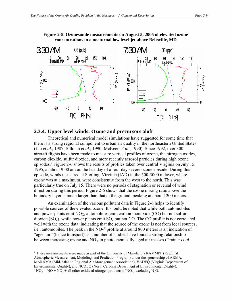
The Nature of the Ozone Air Quality Problem in the Northeast: A Conceptual Description Page 2-9
Figure 2-5. Ozonesonde measurements on August 5, 2005 of elevated ozone concentrations in a nocturnal low level jet above Beltsville, MD
2.3.4. Upper level winds: Ozone and precursors aloft Theoretical and numerical model simulations have suggested for some time that
there is a strong regional component to urban air quality in the northeastern United States (Liu et al., 1987; Sillman et al., 1990; McKeen et al., 1990). Since 1992, over 300 aircraft flights have been made to measure vertical profiles of ozone, the nitrogen oxides, carbon dioxide, sulfur dioxide, and more recently aerosol particles during high ozone episodes.d Figure 2-6 shows the results of profiles taken over central Virginia on July 15, 1995, at about 9:00 am on the last day of a four day severe ozone episode. During this episode, winds measured at Sterling, Virginia (IAD) in the 500-3000 m layer, where ozone was at a maximum, were consistently from the west to the north. This was particularly true on July 15. There were no periods of stagnation or reversal of wind direction during this period. Figure 2-6 shows that the ozone mixing ratio above the boundary layer is much larger than that at the ground, peaking at about 1200 meters.
An examination of the various pollutant data in Figure 2-6 helps to identify possible sources of the elevated ozone. It should be noted that while both automobiles and power plants emit NOX, automobiles emit carbon monoxide (CO) but not sulfur dioxide (SO2), while power plants emit SO2 but not CO. The CO profile is not correlated well with the ozone data, indicating that the source of the ozone is not from local sources, i.e., automobiles. The peak in the NOY
e profile at around 800 meters is an indication of “aged air” (hence transport) as a number of studies have found a strong relationship between increasing ozone and NOY in photochemically aged air masses (Trainer et al.,
d These measurements were made as part of the University of Maryland’s RAMMPP (Regional Atmospheric Measurement, Modeling, and Prediction Program) under the sponsorship of ARMA, MARAMA (Mid-Atlantic Regional Air Management Association), VADEQ (Virginia Department of Environmental Quality), and NCDEQ (North Carolina Department of Environmental Quality). e NOY = NO + NO2 + all other oxidized nitrogen products of NOX, excluding N2O.
7:30AM3:30AM
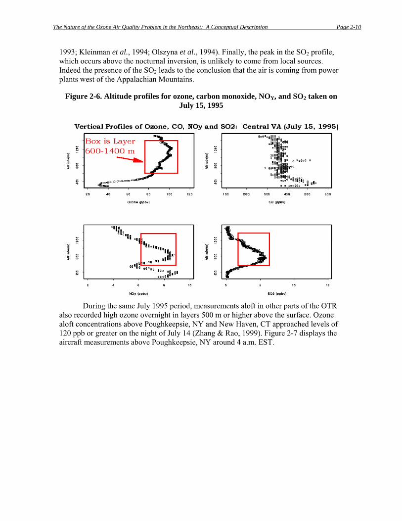
The Nature of the Ozone Air Quality Problem in the Northeast: A Conceptual Description Page 2-10
1993; Kleinman et al., 1994; Olszyna et al., 1994). Finally, the peak in the SO2 profile, which occurs above the nocturnal inversion, is unlikely to come from local sources. Indeed the presence of the SO2 leads to the conclusion that the air is coming from power plants west of the Appalachian Mountains.
Figure 2-6. Altitude profiles for ozone, carbon monoxide, NOY, and SO2 taken on July 15, 1995
During the same July 1995 period, measurements aloft in other parts of the OTR
also recorded high ozone overnight in layers 500 m or higher above the surface. Ozone aloft concentrations above Poughkeepsie, NY and New Haven, CT approached levels of 120 ppb or greater on the night of July 14 (Zhang & Rao, 1999). Figure 2-7 displays the aircraft measurements above Poughkeepsie, NY around 4 a.m. EST.
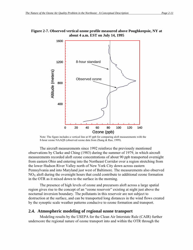
The Nature of the Ozone Air Quality Problem in the Northeast: A Conceptual Description Page 2-11
Figure 2-7. Observed vertical ozone profile measured above Poughkeepsie, NY at about 4 a.m. EST on July 14, 1995
0 20 40 60 80 100 120 140Ozone (ppb)
1600
1200
800
400
Alti
tude
(met
ers)
8-hour standard
Observed ozone
0 20 40 60 80 100 120 140Ozone (ppb)
1600
1200
800
400
Alti
tude
(met
ers)
8-hour standard
Observed ozone
Note: The figure includes a vertical line at 85 ppb for comparing aloft measurements with the 8-hour ozone NAAQS (observed ozone data from Zhang & Rao, 1999).
The aircraft measurements since 1992 reinforce the previously mentioned
observations by Clarke and Ching (1983) during the summer of 1979, in which aircraft measurements recorded aloft ozone concentrations of about 90 ppb transported overnight from eastern Ohio and entering into the Northeast Corridor over a region stretching from the lower Hudson River Valley north of New York City down across eastern Pennsylvania and into Maryland just west of Baltimore. The measurements also observed NOX aloft during the overnight hours that could contribute to additional ozone formation in the OTR as it mixed down to the surface in the morning.
The presence of high levels of ozone and precursors aloft across a large spatial region gives rise to the concept of an “ozone reservoir” existing at night just above the nocturnal inversion boundary. The pollutants in this reservoir are not subject to destruction at the surface, and can be transported long distances in the wind flows created by the synoptic scale weather patterns conducive to ozone formation and transport.
2.4. Atmospheric modeling of regional ozone transport Modeling results by the USEPA for the Clean Air Interstate Rule (CAIR) further
underscore the regional nature of ozone transport into and within the OTR through the
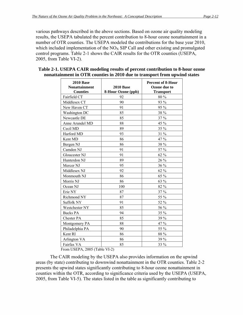
The Nature of the Ozone Air Quality Problem in the Northeast: A Conceptual Description Page 2-12
various pathways described in the above sections. Based on ozone air quality modeling results, the USEPA tabulated the percent contribution to 8-hour ozone nonattainment in a number of OTR counties. The USEPA modeled the contributions for the base year 2010, which included implementation of the NOX SIP Call and other existing and promulgated control programs. Table 2-1 shows the CAIR results for the OTR counties (USEPA, 2005, from Table VI-2).
Table 2-1. USEPA CAIR modeling results of percent contribution to 8-hour ozone nonattainment in OTR counties in 2010 due to transport from upwind states
2010 Base Nonattainment
Counties 2010 Base
8-Hour Ozone (ppb)
Percent of 8-Hour Ozone due to
Transport Fairfield CT 92 80 % Middlesex CT 90 93 % New Haven CT 91 95 % Washington DC 85 38 % Newcastle DE 85 37 % Anne Arundel MD 88 45 % Cecil MD 89 35 % Harford MD 93 31 % Kent MD 86 47 % Bergen NJ 86 38 % Camden NJ 91 57 % Gloucester NJ 91 62 % Hunterdon NJ 89 26 % Mercer NJ 95 36 % Middlesex NJ 92 62 % Monmouth NJ 86 65 % Morris NJ 86 63 % Ocean NJ 100 82 % Erie NY 87 37 % Richmond NY 87 55 % Suffolk NY 91 52 % Westchester NY 85 56 % Bucks PA 94 35 % Chester PA 85 39 % Montgomery PA 88 47 % Philadelphia PA 90 55 % Kent RI 86 88 % Arlington VA 86 39 % Fairfax VA 85 33 %
From USEPA, 2005 (Table VI-2)
The CAIR modeling by the USEPA also provides information on the upwind areas (by state) contributing to downwind nonattainment in the OTR counties. Table 2-2 presents the upwind states significantly contributing to 8-hour ozone nonattainment in counties within the OTR, according to significance criteria used by the USEPA (USEPA, 2005, from Table VI-5). The states listed in the table as significantly contributing to

The Nature of the Ozone Air Quality Problem in the Northeast: A Conceptual Description Page 2-13
downwind ozone nonattainment in the OTR counties include states outside of the OTR, indicating the broad regional scale of the ozone transport problem.
Table 2-2. USEPA CAIR modeling results of upwind states that make a significant contribution to 8-hour ozone in downwind OTR nonattainment counties Downwind
State/County Upwind States CT Middlesex MA NJ NY OH PA VA CT New Haven MD/DC NJ NY OH PA VA WV CT Fairfield MD/DC NJ NY OH PA VA WV District of Columbia MD/DC OH PA VA DE New Castle MD/DC MI NC OH PA VA WV MD Harford NC OH PA VA WV MD Kent MI NC OH PA VA WV MD Cecil MI OH PA VA WV MD Anne Arundel MI NC OH PA VA WV NJ Ocean DE MD/DC MI NY OH PA VA WV NJ Bergen MD/DC MI OH PA VA WV NJ Gloucester DE MD/DC MI OH PA VA WV NJ Morris DE MD/DC MI NY OH PA VA WV NJ Middlesex DE MD/DC MI NY OH PA VA WV NJ Hunterdon DE MD/DC OH PA VA WV NJ Camden DE MD/DC MI OH PA VA WV NJ Mercer DE MD/DC MI NY OH PA VA WV NJ Monmouth DE MD/DC MI NY OH PA VA WV NY Erie MD/DC MI NJ PA VA WI NY Westchester MD/DC NJ OH PA VA WV NY Richmond MD/DC MI NJ PA VA WV NY Suffolk CT DE MD/DC MI NC NJ OH PA VA WV PA Montgomery DE MD/DC NJ OH WV PA Philadelphia DE MD/DC MI NJ OH VA WV PA Chester DE MD/DC MI NJ OH VA WV PA Bucks DE MD/DC MI NJ OH VA WV RI Kent CT MA NJ NY OH PA VA VA Arlington MD/DC OH PA VA Fairfax MD/DC OH PA WV
From USEPA, 2005 (Table VI-5). States are listed alphabetically and not according to order of influence.
While the USEPA modeled 40 eastern U.S. counties as in nonattainment of the 8-hour ozone NAAQS in the 2010 base year (including counties not in the OTR), it projected that only three of those 40 counties would come into attainment by 2010 with the additional NOX reductions of CAIR (USEPA, 2005, p. 58). The USEPA modeling does predict that ozone will be lower in the remaining nonattainment counties by 2010 due to CAIR, with additional counties coming into attainment by 2015. The CAIR reductions, therefore, will bring the OTR nonattainment counties closer to attainment by 2010, but will not result in attainment for a large majority of OTR counties predicted to be in nonattainment in 2010 prior to implementation of CAIR.
The Nature of the Ozone Air Quality Problem in the Northeast: A Conceptual Description Page 2-14
2.5. Summary This section has summarized current knowledge of the meteorological processes
that affect local ozone levels within the OTR. A conceptual description of transport within the OTR can be divided into three principle components: ground level transport at the surface, transport by the nocturnal low level jet, and transport aloft. All three modes of transport depend on the location of the high pressure system. Ground level transport is the result of interaction between the synoptic flow and local effects, such as the sea breeze and the Appalachian lee side trough. Transport within the OTR can occur by the nocturnal low level jet that forms late at night or in the very early morning hours. This phenomenon is a result of the differential heating of the air between the Appalachian Mountains and the Atlantic Ocean. It has been observed throughout the Eastern Seaboard from Georgia to Maine. The nocturnal low level jet can transport ozone that formed within the OTR or was transported into the OTR from outside the region. Transport aloft is dominated by the anti-cyclonic flow around a high pressure system, which can lead to transport of an ozone reservoir into the OTR created by emissions in areas that lie outside the OTR. Local emissions within the OTR add to the polluted air mixing down from above that arrived from more distant locations.
Atmospheric modeling by the USEPA underscores the observations that the OTR’s ozone problem has contributions from outside and upwind of the region. Pollution sources in the Ohio River Valley and the Southeast significantly contribute to ozone nonattainment problems in various portions of the OTR.

The Nature of the Ozone Air Quality Problem in the Northeast: A Conceptual Description Page 2-15
References Clarke, J.F., and J.K.S. Ching. “Aircraft observations of regional transport of ozone in the northeastern United States.” Atmos. Envt. 17, 1703-1712, 1983. Gaza, R.S. “Mesoscale meteorology and high ozone in the northeast United States.” J. Applied Meteor. 37, 961-977, 1998. Hudson, R. “A Conceptual Model for Ozone Transport.” University of Maryland, Dept. of Atmospheric and Oceanic Science. Prepared for the Ozone Transport Commission. Draft Nov. 29, 2005. Kleinman, L., Y.N. Lee, S. Springston, L. Nunnermacker, X. Zhou, R. Brown, K. Hallock, P. Klotz, D. Leahy, J. Lee, and L. Newman. “Ozone Formation at a Rural Site in the Southeastern United States.” J. Geophys. Res. 99, 3469-3482, 1994. Kleinman, L., W.F. Ryan, P.H. Daum, S.R. Springston, Y.-N. Lee, L.J. Nunnermacker, and J. Weinstein-Lloyd. “An ozone episode in the Philadelphia metropolitan area.” J. Geophys. Res. 109, D20302, doi:10.1029/2004JD004563, 2004. Liu, S. C., M. Trainer, F. C. Fehsenfeld, D. D. Parrish, E. J. Williams, D. W. Fahey, G. Hubler, and P. C. Murphy. “Ozone production in the rural troposphere and the implications for regional and global ozone distributions.” J. Geophys. Res. 92, 4191–4207, 1987. Lutgens, F., and E. Tarbuck. The Atmosphere: An Introduction to Meteorology, 8th ed., 512 pp., Prentice Hall, Upper Saddle River, New Jersey, 2001. MARAMA (Mid-Atlantic Regional Air Management Association). A guide to mid-Atlantic regional air quality. MARAMA. Baltimore, MD, pp. 2-3, 2005 (available on-line at www.marama.org/reports). McKeen, S. A., M. Trainer, E. Y. Hsie, R. K. Tallamraju, and S. C. Liu. “On the indirect determination of atmospheric OH radical concentrations from reactive hydrocarbon measurements.” J. Geophys. Res. 95, 7493–7500, 1990. NARSTO. An Assessment of Tropospheric Ozone Pollution. NARSTO, July 2000. Olszyna, K.J., E.M. Bailey, R. Simonaitis and J.F. Meagher. “O3 and NOy Relationships at a Rural Site.” J. Geophys. Res. 99, 14,557-14,563, 1994. Ryan, W.F. and R.R. Dickerson. “Regional transport of pollutants and implications for 8-hour ozone non-attainment areas in Maryland.” Report prepared for the Maryland Department of the Environment, Final version 2.2, 2000.
The Nature of the Ozone Air Quality Problem in the Northeast: A Conceptual Description Page 2-16
Ryan, W.F. “The low level jet in Maryland: Profiler observations and preliminary climatology.” Report prepared for the Maryland Department of the Environment, Air and Radiation Administration, 2004. Sillman, S., J. A. Logan, and S. C. Wofsy. “A regional scale model for ozone in the United States with subgrid representation of urban and power plant plumes.” J. Geophys. Res. 95, 5731–5748, 1990. Sjostedt, D.W., J.T. Sigmon, and S.J. Colucci. “The Carolina nocturnal low-level jet: Synoptic climatology and a case study.” Weather and Forecasting. 5, 404-415, 1990. Stoeckenius, T. and Kemball-Cook, S. “Determination of representativeness of 2002 ozone season for ozone transport region SIP modeling.” Final Report prepared for the Ozone Transport Commission, 2005. Trainer, M., D.D. Parrish, M.P. Buhr, R.B. Norton, F.C. Fehsenfeld, K.G. Anlauf, J.W. Bottenheim, Y.Z. Tang, H.A. Wiebe, J.M. Roberts, R.L. Tanner, L. Newman, V.C. Bowersox, J.F. Meagher, K.J. Olszyna, M.O. Rodgers, T. Wang, H. Berresheim, K.L. Demerjian, and U.K. Roychowdhury. “Correlation of Ozone with NOy in Photochemically Aged Air.” J. Geophys. Res. 98, 2917-2925, 1993. Weisman, R.A. “An observational study of warm season southern Appalachian lee troughs. Part I: Boundary layer circulation.” Monthly Weather Review. 118, 950-962, 1990. Woodman, M.F., D.T. Nguyen, D.J. Krask, E. Joseph, V. Davis, R. Hoff, R. Rogers, M.G. Seybold. “Maryland Ozonesonde Campaign 2005.” Poster at EPA National Air Quality Conference, San Antonio, TX, 2006. Zhang J. and S.T. Rao. “The role of vertical mixing in the temporal evolution of ground-level ozone concentrations.” J. Applied Meteor. 38, 1674-1691, 1999.
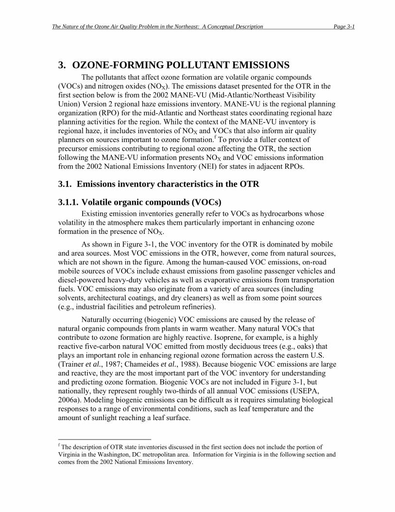
The Nature of the Ozone Air Quality Problem in the Northeast: A Conceptual Description Page 3-1
3. OZONE-FORMING POLLUTANT EMISSIONS The pollutants that affect ozone formation are volatile organic compounds
(VOCs) and nitrogen oxides (NOX). The emissions dataset presented for the OTR in the first section below is from the 2002 MANE-VU (Mid-Atlantic/Northeast Visibility Union) Version 2 regional haze emissions inventory. MANE-VU is the regional planning organization (RPO) for the mid-Atlantic and Northeast states coordinating regional haze planning activities for the region. While the context of the MANE-VU inventory is regional haze, it includes inventories of NOX and VOCs that also inform air quality planners on sources important to ozone formation.f To provide a fuller context of precursor emissions contributing to regional ozone affecting the OTR, the section following the MANE-VU information presents NOX and VOC emissions information from the 2002 National Emissions Inventory (NEI) for states in adjacent RPOs.
3.1. Emissions inventory characteristics in the OTR
3.1.1. Volatile organic compounds (VOCs) Existing emission inventories generally refer to VOCs as hydrocarbons whose
volatility in the atmosphere makes them particularly important in enhancing ozone formation in the presence of NOX.
As shown in Figure 3-1, the VOC inventory for the OTR is dominated by mobile and area sources. Most VOC emissions in the OTR, however, come from natural sources, which are not shown in the figure. Among the human-caused VOC emissions, on-road mobile sources of VOCs include exhaust emissions from gasoline passenger vehicles and diesel-powered heavy-duty vehicles as well as evaporative emissions from transportation fuels. VOC emissions may also originate from a variety of area sources (including solvents, architectural coatings, and dry cleaners) as well as from some point sources (e.g., industrial facilities and petroleum refineries).
Naturally occurring (biogenic) VOC emissions are caused by the release of natural organic compounds from plants in warm weather. Many natural VOCs that contribute to ozone formation are highly reactive. Isoprene, for example, is a highly reactive five-carbon natural VOC emitted from mostly deciduous trees (e.g., oaks) that plays an important role in enhancing regional ozone formation across the eastern U.S. (Trainer et al., 1987; Chameides et al., 1988). Because biogenic VOC emissions are large and reactive, they are the most important part of the VOC inventory for understanding and predicting ozone formation. Biogenic VOCs are not included in Figure 3-1, but nationally, they represent roughly two-thirds of all annual VOC emissions (USEPA, 2006a). Modeling biogenic emissions can be difficult as it requires simulating biological responses to a range of environmental conditions, such as leaf temperature and the amount of sunlight reaching a leaf surface.
f The description of OTR state inventories discussed in the first section does not include the portion of Virginia in the Washington, DC metropolitan area. Information for Virginia is in the following section and comes from the 2002 National Emissions Inventory.
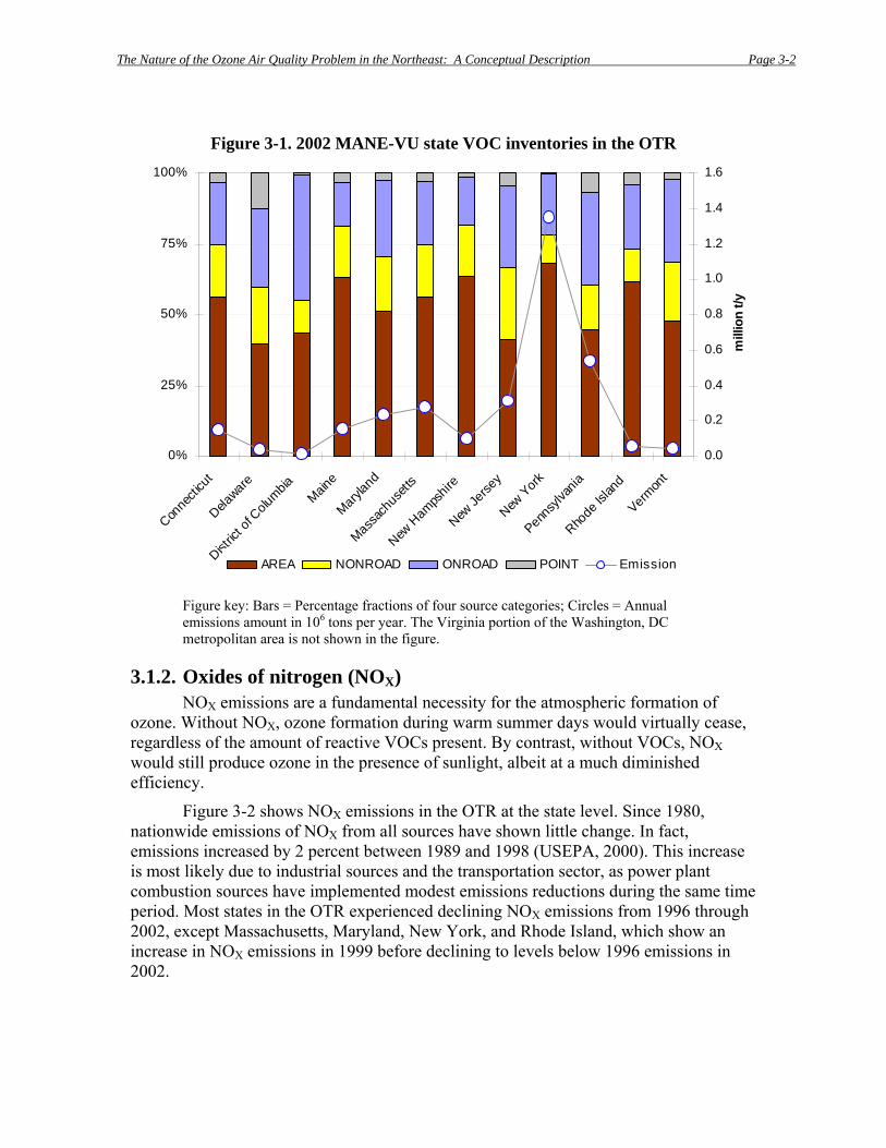
The Nature of the Ozone Air Quality Problem in the Northeast: A Conceptual Description Page 3-2
Figure 3-1. 2002 MANE-VU state VOC inventories in the OTR
0%
25%
50%
75%
100%
Conne
cticu
t
Delaware
Distric
t of C
olumbia
Maine
Marylan
d
Massa
chus
etts
New H
amps
hire
New Je
rsey
New York
Penns
ylvan
ia
Rhode
Islan
d
Vermon
t
mill
ion
t/y
0.0
0.2
0.4
0.6
0.8
1.0
1.2
1.4
1.6
AREA NONROAD ONROAD POINT Emission
Figure key: Bars = Percentage fractions of four source categories; Circles = Annual emissions amount in 106 tons per year. The Virginia portion of the Washington, DC metropolitan area is not shown in the figure.
3.1.2. Oxides of nitrogen (NOX) NOX emissions are a fundamental necessity for the atmospheric formation of
ozone. Without NOX, ozone formation during warm summer days would virtually cease, regardless of the amount of reactive VOCs present. By contrast, without VOCs, NOX would still produce ozone in the presence of sunlight, albeit at a much diminished efficiency.
Figure 3-2 shows NOX emissions in the OTR at the state level. Since 1980, nationwide emissions of NOX from all sources have shown little change. In fact, emissions increased by 2 percent between 1989 and 1998 (USEPA, 2000). This increase is most likely due to industrial sources and the transportation sector, as power plant combustion sources have implemented modest emissions reductions during the same time period. Most states in the OTR experienced declining NOX emissions from 1996 through 2002, except Massachusetts, Maryland, New York, and Rhode Island, which show an increase in NOX emissions in 1999 before declining to levels below 1996 emissions in 2002.
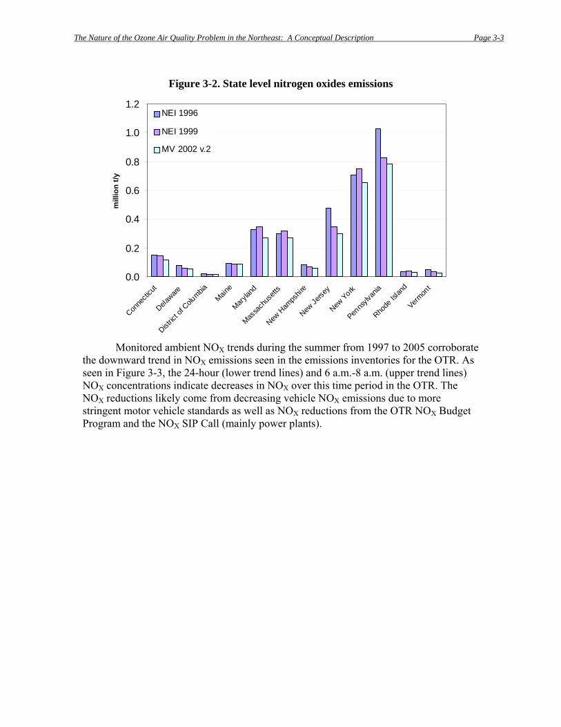
The Nature of the Ozone Air Quality Problem in the Northeast: A Conceptual Description Page 3-3
Figure 3-2. State level nitrogen oxides emissions
0.0
0.2
0.4
0.6
0.8
1.0
1.2
Conne
cticu
t
Delaware
Distric
t of C
olumbia
Maine
Marylan
d
Massa
chus
etts
New H
amps
hire
New Je
rsey
New York
Penns
ylvan
ia
Rhode
Islan
d
Vermon
t
mill
ion
t/yNEI 1996
NEI 1999
MV 2002 v.2
Monitored ambient NOX trends during the summer from 1997 to 2005 corroborate
the downward trend in NOX emissions seen in the emissions inventories for the OTR. As seen in Figure 3-3, the 24-hour (lower trend lines) and 6 a.m.-8 a.m. (upper trend lines) NOX concentrations indicate decreases in NOX over this time period in the OTR. The NOX reductions likely come from decreasing vehicle NOX emissions due to more stringent motor vehicle standards as well as NOX reductions from the OTR NOX Budget Program and the NOX SIP Call (mainly power plants).
The Nature of the Ozone Air Quality Problem in the Northeast: A Conceptual Description Page 3-4
Figure 3-3. Plot of monitored NOX trends in OTR during 1997-2005
JUNE, JULY & AUGUST 1997-2005 OTC AVERAGE NOx CONCENTRATIONS
10
15
20
25
30
35
40
45
50
1997
1998
1999
2000
2001
2002
2003
2004
2005
1997
1998
1999
2000
2001
2002
2003
2004
2005
1997
1998
1999
2000
2001
2002
2003
2004
2005
Ave
rage
Con
cent
ratio
n (p
pb)
.
JUN (all hrs)JUL (all hrs)AUG (all hrs)JUN (06-08 EST)JUL (06-08 EST)AUG (06-08 EST)
Note: Upper trend lines correspond to ambient NOX measured from 0600-0800 EST in the morning. Lower trend lines correspond to NOX measured over entire day (created by Tom Downs, Maine Department of Environmental Protection).
Power plants and mobile sources generally dominate state and national NOX
emissions inventories. Nationally, power plants account for more than one-quarter of all NOX emissions, amounting to over six million tons. The electric sector plays an even larger role, however, in parts of the industrial Midwest where high NOX emissions have a particularly significant power plant contribution. By contrast, mobile sources dominate the NOX inventories for more urbanized mid-Atlantic and New England states to a far greater extent, as shown in Figure 3-4. In these states, on-road mobile sources — a category that mainly includes highway vehicles — represent the most significant NOX source category. Emissions from non-road (i.e., off-highway) mobile sources, primarily diesel-fired engines, also represent a substantial fraction of the inventory.
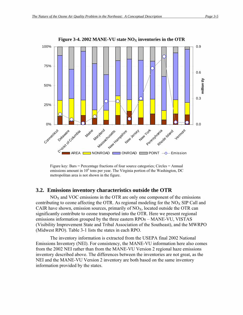
The Nature of the Ozone Air Quality Problem in the Northeast: A Conceptual Description Page 3-5
Figure 3-4. 2002 MANE-VU state NOX inventories in the OTR
0%
25%
50%
75%
100%
Conne
cticu
t
Delaware
Distric
t of C
olumbia
Maine
Marylan
d
Massa
chus
etts
New H
amps
hire
New Je
rsey
New York
Penns
ylvan
ia
Rhode
Islan
d
Vermon
t
mill
ion
t/y
0.0
0.3
0.6
0.9
AREA NONROAD ONROAD POINT Emission
Figure key: Bars = Percentage fractions of four source categories; Circles = Annual emissions amount in 106 tons per year. The Virginia portion of the Washington, DC metropolitan area is not shown in the figure.
3.2. Emissions inventory characteristics outside the OTR NOX and VOC emissions in the OTR are only one component of the emissions
contributing to ozone affecting the OTR. As regional modeling for the NOX SIP Call and CAIR have shown, emission sources, primarily of NOX, located outside the OTR can significantly contribute to ozone transported into the OTR. Here we present regional emissions information grouped by the three eastern RPOs – MANE-VU, VISTAS (Visibility Improvement State and Tribal Association of the Southeast), and the MWRPO (Midwest RPO). Table 3-1 lists the states in each RPO.
The inventory information is extracted from the USEPA final 2002 National Emissions Inventory (NEI). For consistency, the MANE-VU information here also comes from the 2002 NEI rather than from the MANE-VU Version 2 regional haze emissions inventory described above. The differences between the inventories are not great, as the NEI and the MANE-VU Version 2 inventory are both based on the same inventory information provided by the states.
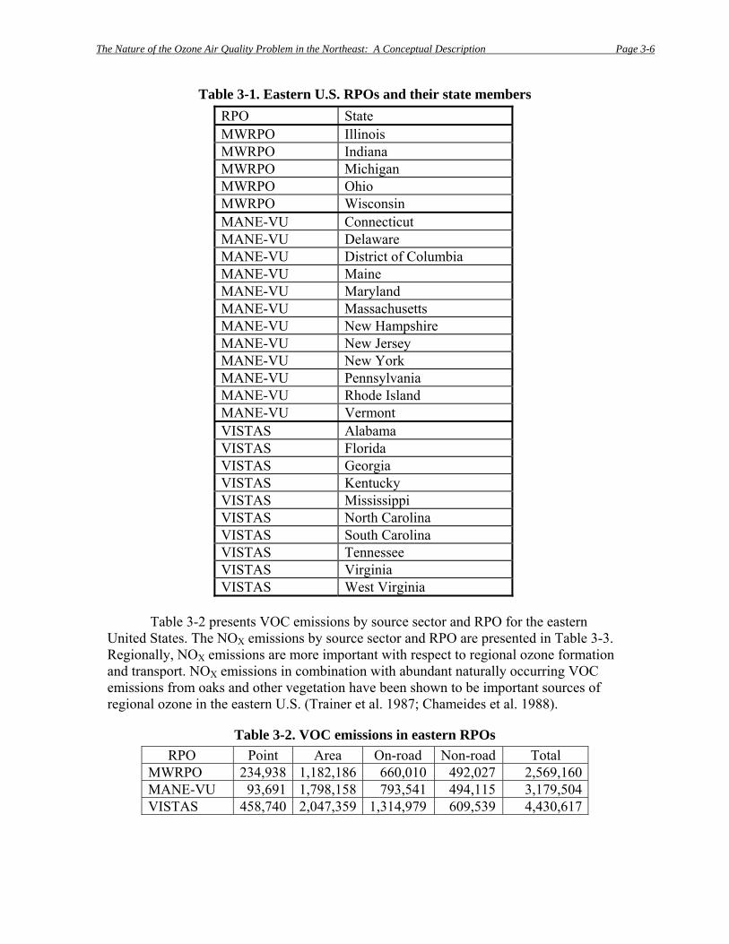
The Nature of the Ozone Air Quality Problem in the Northeast: A Conceptual Description Page 3-6
Table 3-1. Eastern U.S. RPOs and their state members RPO State MWRPO Illinois MWRPO Indiana MWRPO Michigan MWRPO Ohio MWRPO Wisconsin MANE-VU Connecticut MANE-VU Delaware MANE-VU District of Columbia MANE-VU Maine MANE-VU Maryland MANE-VU Massachusetts MANE-VU New Hampshire MANE-VU New Jersey MANE-VU New York MANE-VU Pennsylvania MANE-VU Rhode Island MANE-VU Vermont VISTAS Alabama VISTAS Florida VISTAS Georgia VISTAS Kentucky VISTAS Mississippi VISTAS North Carolina VISTAS South Carolina VISTAS Tennessee VISTAS Virginia VISTAS West Virginia
Table 3-2 presents VOC emissions by source sector and RPO for the eastern
United States. The NOX emissions by source sector and RPO are presented in Table 3-3. Regionally, NOX emissions are more important with respect to regional ozone formation and transport. NOX emissions in combination with abundant naturally occurring VOC emissions from oaks and other vegetation have been shown to be important sources of regional ozone in the eastern U.S. (Trainer et al. 1987; Chameides et al. 1988).
Table 3-2. VOC emissions in eastern RPOs RPO Point Area On-road Non-road Total
MWRPO 234,938 1,182,186 660,010 492,027 2,569,160 MANE-VU 93,691 1,798,158 793,541 494,115 3,179,504 VISTAS 458,740 2,047,359 1,314,979 609,539 4,430,617

The Nature of the Ozone Air Quality Problem in the Northeast: A Conceptual Description Page 3-7
Table 3-3. NOX emissions in eastern RPOs RPO Point Area On-road Non-road Total
MWRPO 1,437,284 184,790 1,290,178 723,844 3,636,096 MANE-VU 680,975 268,997 1,297,357 534,454 2,781,783 VISTAS 2,094,228 266,848 2,160,601 812,615 5,334,293
3.3. Are NOX or VOC control strategies most effective at reducing ozone?
The effectiveness of a NOX-focused or VOC-focused control strategy to reduce ozone is not constant by location or emissions; rather it is a changing chemical characteristic of an air parcel affecting a particular location. As a result, the effectiveness of a NOX or VOC-focused control strategy can vary within an air parcel as it dynamically evolves over time with transport, dispersion, and photochemical aging (NARSTO, 2000).
On a regional basis, OTAG, CAIR and other modeling studies have consistently shown that NOX reductions have the greatest impact on regional ozone concentrations, while VOC reductions have more local impacts. This is largely a result of significant naturally occurring VOC emissions (especially isoprene) in large forested regions of the eastern U.S. Real-world results from regional NOX reductions at power plants (i.e., the NOX SIP Call) are now indicating that significant ozone reductions are occurring on a regional basis as a result of regional NOX strategies. A recent USEPA report finds a strong association between areas with the greatest NOX emission reductions due to the NOX SIP Call and downwind sites exhibiting the greatest improvement in ozone in 2005 (USEPA, 2006b).
As a general rule, VOC reductions may be effective at reducing urban-scale ozone pollution in lieu of or in combination with local NOX reductions, while regional NOX controls are most effective at reducing regional ozone. While a general rule can be outlined in evaluating the potential effectiveness of NOX and VOC-focused control strategies, the optimal strategy for a specific location will depend on the particular circumstances of that location. Exceptions to a VOC-only strategy for an urban area can occur when the urban area has large natural VOC emissions, ozone is transported from upwind, or there is recirculation of aged local pollution (e.g., sea breeze effect). Furthermore, because the conditions causing individual ozone episodes can vary, a given urban area may change in sensitivity between a NOX and VOC-focused strategy depending on a particular episode’s conditions (NARSTO, 2000). Therefore, the appropriate combination of VOC and NOX controls at the local level depends on local circumstances with the realization that a single approach focusing on NOX or VOC-only controls is not necessarily effective for all episode types. It is clear, however, that regional NOX reductions provide regional ozone reductions, and this will influence ozone levels being transported into local urban areas.
The Nature of the Ozone Air Quality Problem in the Northeast: A Conceptual Description Page 3-8
3.4. Summary There are large emissions of VOCs and NOX within and outside the OTR that
contribute to local and regional ozone problems. Naturally occurring VOC emissions play an important role in combination with human-caused NOX emissions in forming regional ozone across large sections of the eastern U.S. Regional NOX control strategies are demonstrating success in reducing regional ozone. On a more local scale, some combination of VOC and NOX controls may be needed, with the specific combination dependent upon local circumstances.
The Nature of the Ozone Air Quality Problem in the Northeast: A Conceptual Description Page 3-9
References
Chameides, W.L., R.W. Lindsay, J. Richardson, and C.S. Kiang. “The role of biogenic hydrocarbons in urban photochemical smog: Atlanta as a case study.” Science 241, 1473-1475, 1988. NARSTO. An Assessment of Tropospheric Ozone Pollution. NARSTO, July 2000. Trainer, M., E.J. Williams, D.D. Parrish, M.P. Buhr, E.J. Allwine, H.H. Westberg, F.C. Fehsenfeld, and S.C. Liu. “Models and observations of the impact of natural hydrocarbons on rural ozone.” Nature 329, 705-707, 1987. USEPA. National Air Quality and Emission Trends Report, 1998, EPA 454/R-00-003, available online: http://www.epa.gov/oar/aqtrnd98/, 2000. USEPA. 2002 Final National Emissions Inventory (NEI), available online: ftp://ftp.epa.gov/EmisInventory/2002finalnei/, 2006a (accessed October 10, 2006) [The 2002 NEI reports national annual emissions for total anthropogenic VOC emissions as 16.8 million tons, and total biogenic VOC emissions as 41.8 million tons]. USEPA. NOX Budget Trading Program 2005 Compliance and Environmental Results, EPA430-R-06-013, available online: http://www.epa.gov/airmarkets/fednox/, 2006b.
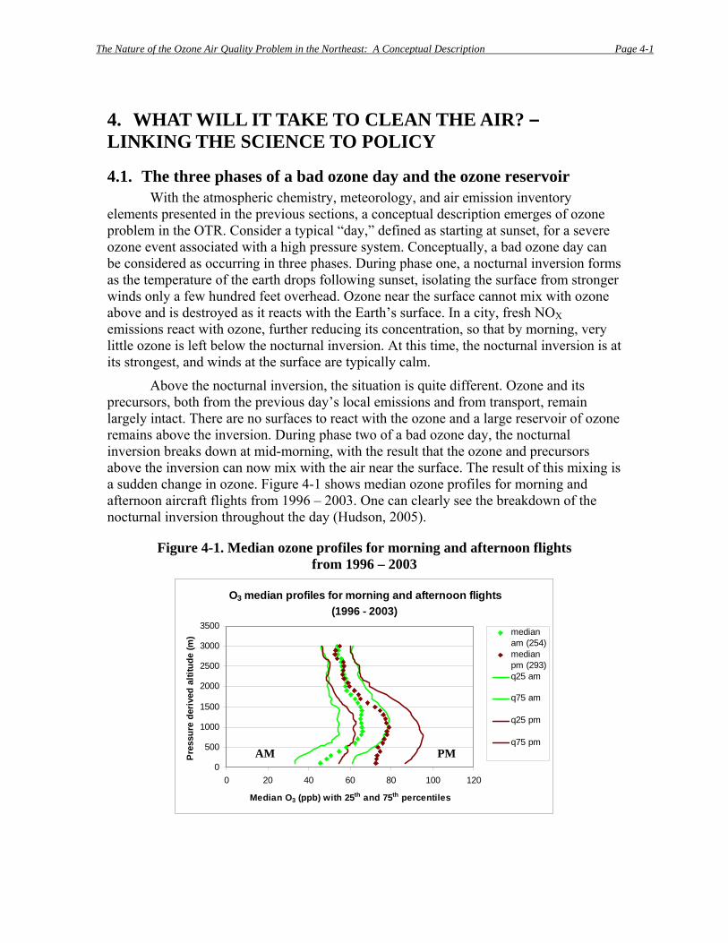
The Nature of the Ozone Air Quality Problem in the Northeast: A Conceptual Description Page 4-1
4. WHAT WILL IT TAKE TO CLEAN THE AIR? – LINKING THE SCIENCE TO POLICY
4.1. The three phases of a bad ozone day and the ozone reservoir With the atmospheric chemistry, meteorology, and air emission inventory
elements presented in the previous sections, a conceptual description emerges of ozone problem in the OTR. Consider a typical “day,” defined as starting at sunset, for a severe ozone event associated with a high pressure system. Conceptually, a bad ozone day can be considered as occurring in three phases. During phase one, a nocturnal inversion forms as the temperature of the earth drops following sunset, isolating the surface from stronger winds only a few hundred feet overhead. Ozone near the surface cannot mix with ozone above and is destroyed as it reacts with the Earth’s surface. In a city, fresh NOX emissions react with ozone, further reducing its concentration, so that by morning, very little ozone is left below the nocturnal inversion. At this time, the nocturnal inversion is at its strongest, and winds at the surface are typically calm.
Above the nocturnal inversion, the situation is quite different. Ozone and its precursors, both from the previous day’s local emissions and from transport, remain largely intact. There are no surfaces to react with the ozone and a large reservoir of ozone remains above the inversion. During phase two of a bad ozone day, the nocturnal inversion breaks down at mid-morning, with the result that the ozone and precursors above the inversion can now mix with the air near the surface. The result of this mixing is a sudden change in ozone. Figure 4-1 shows median ozone profiles for morning and afternoon aircraft flights from 1996 – 2003. One can clearly see the breakdown of the nocturnal inversion throughout the day (Hudson, 2005).
Figure 4-1. Median ozone profiles for morning and afternoon flights from 1996 – 2003
O3 median profiles for morning and afternoon flights (1996 - 2003)
0
500
1000
1500
2000
2500
3000
3500
0 20 40 60 80 100 120
Median O3 (ppb) with 25th and 75th percentiles
Pres
sure
der
ived
alti
tude
(m) median
am (254)medianpm (293)q25 am
q75 am
q25 pm
q75 pmAM PM
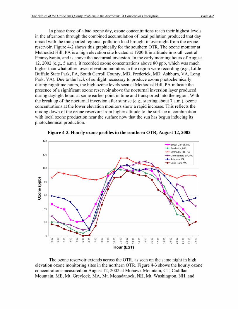
The Nature of the Ozone Air Quality Problem in the Northeast: A Conceptual Description Page 4-2
In phase three of a bad ozone day, ozone concentrations reach their highest levels in the afternoon through the combined accumulation of local pollution produced that day mixed with the transported regional pollution load brought in overnight from the ozone reservoir. Figure 4-2 shows this graphically for the southern OTR. The ozone monitor at Methodist Hill, PA is a high elevation site located at 1900 ft in altitude in south central Pennsylvania, and is above the nocturnal inversion. In the early morning hours of August 12, 2002 (e.g., 5 a.m.), it recorded ozone concentrations above 80 ppb, which was much higher than what other lower elevation monitors in the region were recording (e.g., Little Buffalo State Park, PA, South Carroll County, MD, Frederick, MD, Ashburn, VA, Long Park, VA). Due to the lack of sunlight necessary to produce ozone photochemically during nighttime hours, the high ozone levels seen at Methodist Hill, PA indicate the presence of a significant ozone reservoir above the nocturnal inversion layer produced during daylight hours at some earlier point in time and transported into the region. With the break up of the nocturnal inversion after sunrise (e.g., starting about 7 a.m.), ozone concentrations at the lower elevation monitors show a rapid increase. This reflects the mixing down of the ozone reservoir from higher altitude to the surface in combination with local ozone production near the surface now that the sun has begun inducing its photochemical production.
Figure 4-2. Hourly ozone profiles in the southern OTR, August 12, 2002
0
20
40
60
80
100
120
140
0:00
1:00
2:00
3:00
4:00
5:00
6:00
7:00
8:00
9:00
10:0
0
11:0
0
12:0
0
13:0
0
14:0
0
15:0
0
16:0
0
17:0
0
18:0
0
19:0
0
20:0
0
21:0
0
22:0
0
23:0
0
Hour (EST)
Ozo
ne (p
pb)
South Carroll, MDFrederick, MDMethodist Hill, PALittle Buffalo SP, PAAshburn, VALong Park, VA
The ozone reservoir extends across the OTR, as seen on the same night in high elevation ozone monitoring sites in the northern OTR. Figure 4-3 shows the hourly ozone concentrations measured on August 12, 2002 at Mohawk Mountain, CT, Cadillac Mountain, ME, Mt. Greylock, MA, Mt. Monadanock, NH, Mt. Washington, NH, and

The Nature of the Ozone Air Quality Problem in the Northeast: A Conceptual Description Page 4-3
Whiteface Mountain, NY. As with Methodist Hill, PA on this day, these sites show elevated ozone concentrations during nighttime hours, as compared to lower elevation sites below the nocturnal inversion (e.g., Danbury, CT). By mid-day, however, the nocturnal boundary layer has broken down, mixing the transported ozone from the reservoir above into the locally produced ozone below. Appendix G provides more detail on contributions to the ozone reservoir within and outside the OTR.
Figure 4-3. Hourly ozone profiles in the northern OTR, August 12, 2002
0
20
40
60
80
100
120
140
0:00
1:00
2:00
3:00
4:00
5:00
6:00
7:00
8:00
9:00
10:0
0
11:0
0
12:0
0
13:0
0
14:0
0
15:0
0
16:0
0
17:0
0
18:0
0
19:0
0
20:0
0
21:0
0
22:0
0
23:0
0
Hour (EST)
Ozo
ne (p
pb)
Mohawk Mtn., CTMt. Monadanock, NHMt. Greylock, MAMt. Washington, NHWhiteface Mtn., NYCadillac Mtn., MEDanbury, CT
Data provided by Tom Downs, Maine Department of Environmental Protection.
4.2. Chronology of an ozone episode – August 2002 The chronology of an historical ozone episode occurring in the OTR from August
8 to August 16, 2002 provides a real-world example that pieces together the elements of the ozone conceptual description given in this document. Surface maps from the period provide a synoptic overview of major weather systems that were influencing air quality across the OTR during that time. Meteorological insights combined with ozone concentration information provide a picture of the evolving ozone episode on a day-by-day basis. Figure 4-4, Figure 4-5, and Figure 4-6, respectively, show eight-panel displays of surface weather maps, back trajectories, and 8-hour maximum ozone concentrations from each day. The daily progression shows the formation of high ozone that shifts from west to east, and ultimately northward, during successive days of the episode according to local ozone formation and transport shaped by wind patterns within and outside of the OTR.
The August 2002 episode began with a slow-moving high pressure system centered over the Great Lakes initiating a northerly flow over the OTR on August 8. Over
The Nature of the Ozone Air Quality Problem in the Northeast: A Conceptual Description Page 4-4
the next several days, the high drifted southeastward and became extended across a large part of the eastern U.S., bringing high temperatures to the region. Calm conditions west of the OTR on August 10 were pivotal for the formation of ozone, which first began building in the Ohio River Valley. Over the next four days, 8-hour ozone concentrations climbed well above the 85 ppb (0.08 ppm) NAAQS over a wide area of the OTR. Large parts of the heavily populated Northeast Corridor experienced 8-hour ozone levels above 100 ppb during the height of the episode, which far exceeded the 85 ppb NAAQS.
The following chronology provides a day-by-day evolution of the August 2002 ozone episode. Parts of this description are taken from Ryan (2003).
August 8: A high pressure system over the Great Lakes produces NW-N prevailing surface winds (~4-8 mph) throughout the region. Maximum daily temperatures approach or exceed 80º F.
August 9: Wind speeds fall off but the direction remains NW-N as the high moves into the Pennsylvania-New York region. Temperatures rise as cloud cover declines. Background ozone levels begin to build in the Ohio River Valley with 8-hour maximum concentrations reaching the 60-80 ppb range.
August 10: High pressure is directly over the mid-Atlantic. With dew points still in the mid-50º’s F, the skies are extraordinarily clear throughout the day. Temperatures (except in northern-most areas) approach 90º F while surface-level winds turn to more southerly directions. With high pressure overhead, the back trajectories suggest very light winds and recirculation. Calm conditions through the morning hours in the lower Ohio River Valley promote increasingly higher levels of ozone noted in surface observations – now reaching above the 85 ppb 8-hour ozone NAAQS over much of Indiana, Ohio, and other states along the Ohio River, as well as states around Lake Michigan and large portions of the southeastern U.S. Ozone levels above the 8-hour NAAQS now begin appearing for the first time in the western and southern parts of the OTR.
August 11: Surface high pressure drops slowly southeastward across the mid-Atlantic with the center in western North Carolina drifting to coastal South Carolina during the day. The upper level ridge has also moved east and is located over the mid-Atlantic. Circulation around the high becomes well established. A surface-level trough descends from north of the Great Lakes during the day, passes eastward through the Ohio River Valley and stalls over the Allegheny Mountains and southward. Peak temperatures are in the low to mid-90º’s F. Morning winds are low-to-calm in the area east of the Mississippi – the area of ozone now reaches from eastern Wisconsin to Tennessee and eastward to Georgia up through the Carolinas into the OTR, covering most of Pennsylvania, New York, New Jersey, Connecticut, Rhode Island and Massachusetts. Winds are generally south to southwest as is reflected in the boundary layer back trajectories. The key factor driving local ozone production appears to be a very stable boundary layer. The 8 a.m. sounding at the Washington-Dulles airport shows a very strong low-level inversion from 950-900 mb with a deep residual layer beneath a continuing strong subsidence inversion – now based at 760 mb.
August 12: The upper level ridge remains quasi-stationary with its axis over the mid-Atlantic. The center of high pressure at 850 mb is over North Carolina and Georgia. At the surface, the characteristic Appalachian lee side trough forms. Temperatures exceed
The Nature of the Ozone Air Quality Problem in the Northeast: A Conceptual Description Page 4-5
90º F throughout the OTR except in coastal Maine. Winds are fairly strong from the northwest. This is reflected in the back trajectories that show a shift to westerly transport. Elevated upwind ozone concentrations at 11 a.m. on August 11 occur in the vicinity of the origin of the back trajectories, on the order of 78-86 ppb. Ozone concentrations fall this day west of the Appalachians but increase markedly across the mid-Atlantic. The area of highest ozone has pushed eastward and now extends from southern Maine across central Pennsylvania down through Maryland into the Carolinas, Georgia, and eastern Tennessee. Ozone builds throughout the day as circulation forces it to channel northeast between the stalled trough and a cold front approaching from the Midwest. Some of the highest 8-hour concentrations occur through the central to southern OTR on this day.
August 13: Calm conditions prevail as the trough reaches coastal New Jersey by 8 a.m. Generally clear skies allow temperatures to reach the mid-90º’s F everywhere except in coastal Maine. Dew points, which had been rising since August 8, reach the upper 60º’s F. A morning sounding at the Washington-Dulles airport showed a continuing strong low level inversion with a residual mixed layer to 850 mb ending just beneath a weak secondary inversion. The cap aloft has lifted to ~ 630 mb and the sounding is more unstable compared to previous day’s between the two inversion layers. The Appalachian lee side trough continues in place from late on August 12. As is typically the case, the highest ozone concentrations are found in proximity to this boundary. The highest 8-hour ozone concentrations are along the eastern portions of the OTR from northeastern Virginia through New Jersey, Long Island, Connecticut, and into eastern Massachusetts. By 8 p.m., showers associated with the approaching cold front have reached into Ohio.
August 14: By 8 a.m., the trough has dissipated and the high is moving offshore, resulting in an increasing southerly wind component, which pushes maritime air northward. Dew points remain in the upper 60º’s F and peak temperatures reach into the 90º’s F everywhere and top 100º F in several locations. Ozone concentrations build again, with the highest levels concentrated in the central OTR from eastern Pennsylvania across to Massachusetts. A “hotspot” of ozone appears in upstate New York at the eastern end of Lake Ontario, and may be the result of transport from the west across the lake. Ozone concentrations decrease south and west of Baltimore and along coastal New Jersey as cleaner maritime air pushes in from the south.
August 15: This episode ends in a very different manner than the standard high ozone episode. Instead of the passage of a sharp cold front, this episode ends gradually as cleaner air sweeps north, winds increase, and the atmosphere steadily destabilizes. Ozone concentrations fall across the middle and lower OTR as low level flow becomes more southeast and the Bermuda high fills in westward. The highest levels, still exceeding the 8-hour ozone NAAQS, now occur in the northern reaches of the OTR in upstate New York, Vermont, New Hampshire, and Maine.
August 16: Cloud cover spreads over the region with ozone falling further. The new high building into the upper Midwest pushes the remains of the showers out of the Northeast. A spot of high ozone persists in central New Jersey. This is the last exceedance day in a string of seven exceedance days within the OTR during this extended episode.
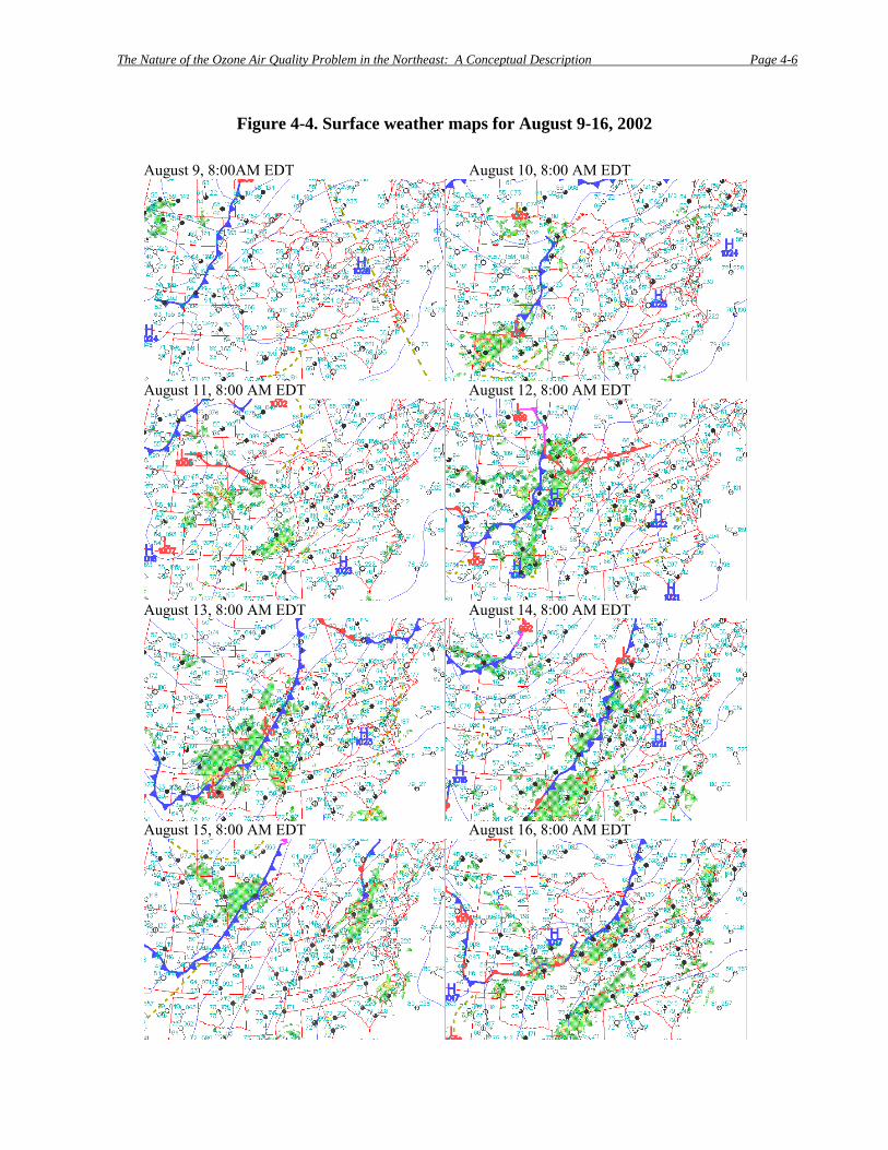
The Nature of the Ozone Air Quality Problem in the Northeast: A Conceptual Description Page 4-6
Figure 4-4. Surface weather maps for August 9-16, 2002
August 9, 8:00AM EDT August 10, 8:00 AM EDT
August 11, 8:00 AM EDT August 12, 8:00 AM EDT
August 13, 8:00 AM EDT August 14, 8:00 AM EDT
August 15, 8:00 AM EDT August 16, 8:00 AM EDT

The Nature of the Ozone Air Quality Problem in the Northeast: A Conceptual Description Page 4-7
Figure 4-5. HYSPLIT 72-hour back trajectories for August 9-16, 2002
Aug 9, 2002 8 am EDTAug 9, 2002 8 am EDT Aug 10, 2002 8 am EDTAug 10, 2002 8 am EDT
Aug 11, 2002 8 am EDTAug 11, 2002 8 am EDT Aug 12, 2002 8 am EDTAug 12, 2002 8 am EDT
Aug 13, 2002 8 am EDTAug 13, 2002 8 am EDT Aug 14, 2002 8 am EDTAug 14, 2002 8 am EDT
Aug 15, 2002 8 am EDTAug 15, 2002 8 am EDT Aug 16, 2002 8 am EDTAug 16, 2002 8 am EDT
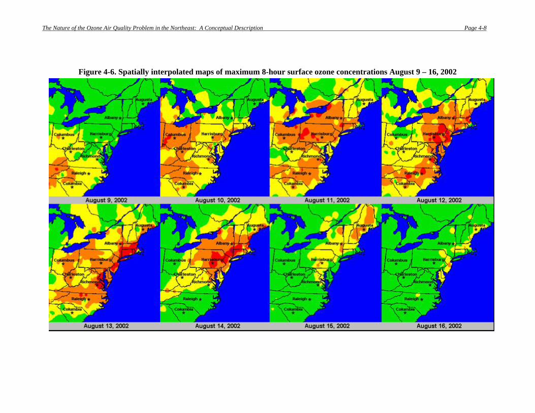
The Nature of the Ozone Air Quality Problem in the Northeast: A Conceptual Description Page 4-8
Figure 4-6. Spatially interpolated maps of maximum 8-hour surface ozone concentrations August 9 – 16, 2002
The Nature of the Ozone Air Quality Problem in the Northeast: A Conceptual Description Page 4-9
4.3. Clean Air Act provisions As is evident from the myriad source regions and transport pathways affecting the
OTR, the regional ozone nonattainment problem presents a significant challenge to air quality planners. To improve air quality, emission reductions of the appropriate pollutants must occur at the appropriate levels (i.e., stringency of controls) and over the appropriate geographic extent. States have primary responsibility for achieving the goals of the Clean Air Act, as they are responsible for developing State Implementation Plans and implementing and enforcing emission reduction programs to meet the health-protective National Ambient Air Quality Standards (NAAQS).
When Congress passed the Clean Air Act Amendments of 1990, it recognized that air pollution transcends political boundaries and that tools for addressing transport must be made available to state and federal governments. Accordingly, several Clean Air Act provisions deal with transported pollution, including: (1) prohibiting the USEPA from approving State Implementation Plans that interfere with another state’s ability to attain or maintain a NAAQS; (2) requiring the USEPA to work with states to prevent emissions that contribute to air pollution in a foreign country; (3) allowing states to form ozone transport regions; (4) requiring states in ozone transport regions to adopt a prescribed set of controls in order to achieve a minimum level of regional emission reductions; and (5) allowing states to petition the USEPA for timely relief from stationary source emissions that interfere with attainment or maintenance of a NAAQS, and requiring the USEPA to act on such petitions within a very short, prescribed timeframe. Taken together, these provisions provide a framework for air quality planning. Its inherent principles are:
• Timely action is critical in order to protect public health; • States must act locally to address air pollution; • While acting locally, states must also consider their impacts downwind in addition
to in-state impacts when developing state implementation plans (SIPs), and ameliorate such impacts through SIPs;
• Regional actions have been and can continue to be effective; • To be effective on a regional level, states working together must work off of a
level playing field.
What the science tells us of the nature of the ozone problem in the OTR supports this framework. The smaller scale weather patterns that affect pollution accumulation and transport underscore the importance of local (in-state) controls for NOX and VOC emissions. Larger synoptic scale weather patterns, and pollution patterns associated with them, support the need for NOX controls across the eastern United States. Studies and characterizations of nocturnal low level jets (i.e., channeled transport) also support the need for local and regional controls on NOX and VOC sources as local and transported pollution from outside the OTR can be entrained in nocturnal low level jets formed during nighttime hours within the OTR. Land, sea, mountain, and valley breezes indicate that there are unique aspects of pollution accumulation and transport that are area-specific and will warrant policy responses at the local and regional levels beyond a one-size-fits-all approach.
The Nature of the Ozone Air Quality Problem in the Northeast: A Conceptual Description Page 4-10
The mix of emission controls is also important for states to consider. While long-range transport of ozone is primarily due to NOX, VOCs are important because they contribute to ozone formation by influencing how efficiently ozone is produced by NOX, particularly within urban centers. While reductions in anthropogenic VOCs will typically have less of an impact on the long-range transport of ozone, they can be effective in reducing ozone in those urban areas where ozone production may be limited by the availability of VOCs. Therefore, a combination of localized VOC reductions in urban centers with additional NOX reductions (from both mobile and point sources) across a larger region will help to reduce ozone and precursors in nonattainment areas as well as their downwind transport across the entire region (NESCAUM, 1997).
4.4. Past regional efforts While states are somewhat limited in their ability to directly affect emissions
reductions beyond their own geo-political boundaries, over the past 15-20 years, the Northeast states have acted regionally with tremendous success. Such efforts have included:
• In 1989, regional low volatility gasoline (i.e., Reid Vapor Pressure pf 9.0 psi) was introduced into the NESCAUM region, resulting in significant VOC reductions;
• In 1994, the California Low Emission Vehicle (LEV) program commenced in the Northeast Corridor as regulations were adopted by Maine, Massachusetts, New York, and Vermont. To date, four additional states have joined the program, which continues to yield reductions in NOX, VOC, CO, and air toxics.
• In 1994, the states of the Ozone Transport Commission agreed to promulgate regional NOX RACT controls and a NOX cap-and-trade program. The adopted regional RACT deadline was 1995. By 1999, the NOX Budget Program was implemented over the 12-state region from Maine to Washington, DC. In 2002, the USEPA reported that the NOX Budget sources “emitted at a level approximately 12 percent below 2001 allocations” (USEPA, 2002). Progress continues with a more stringent cap taking effect in 2003.
• In 1997, eight OTR states petitioned the USEPA under section 126 of the Clean Air Act, requesting NOX emissions reductions on certain stationary sources in the Eastern U.S. In 1999, four more OTR members filed section 126 petitions. The USEPA granted four of the initial eight state petitions in 2000.g
• In 2001, the states of the Ozone Transport Commission agreed to support a suite of model rules for inclusion in SIPs as appropriate to address 1-hour ozone problems. The model rules included controls for: (1) architectural and industrial maintenance coatings; (2) portable fuel containers; (3) consumer products; (4) solvent cleaning; (5) mobile equipment repair and refinishing; and (5) additional
g The initial eight section 126 OTR states were Connecticut, Maine, Massachusetts, New Hampshire, New York, Pennsylvania, Rhode Island, and Vermont. The additional four OTR members filing section 126 petitions were Delaware, the District of Columbia, Maryland, and New Jersey. The four granted petitions were from Connecticut, Massachusetts, New York, and Pennsylvania.

The Nature of the Ozone Air Quality Problem in the Northeast: A Conceptual Description Page 4-11
NOX controls for industrial boilers, cement kilns, stationary reciprocating engines, and stationary combustion engines.
These regional efforts have led the way for similar broader regional and national programs. For mobile sources, the USEPA promulgated its federal Reformulated Gasoline Program in 1995 and the National LEV program in 1998. For stationary sources, the USEPA announced in 1997 that it would expand the OTR NOX Budget Program through the NOX SIP Call, which included 22 states and NOX caps in place by 2003. The NOX SIP Call also served as a response to the states’ Section 126 petitions under the Clean Air Act.
In 2005, the USEPA took a further step to address the regional ozone problem by issuing the Clean Air Interstate Rule (CAIR), which requires additional NOX reductions in 25 eastern states and the District of Columbia. The USEPA projects that CAIR will achieve NOX reductions of 2 million tons in 2015, a 61% decrease from 2003 levels. This will be a significant step forward in improving air quality, but the time allowed to achieve these reductions is later than the deadline many eastern states are facing to meet the current 8-hour ozone NAAQS. This, therefore, only partially provides the OTR with a regional measure that helps achieve the Clean Air Act’s goal of attaining the ozone air quality health standard within the Act’s mandatory deadlines.
4.5. Summary: Building upon success A conceptual understanding of ozone as a regional problem in the OTR and
throughout the eastern U.S. is now well established. With this evolution in understanding, regional approaches to the ozone problem are now underway, starting with the 1990 Clean Air Act Amendments that created the Ozone Transport Region. This initial regional approach, however, did not include large source regions outside of the OTR containing many large coal-fired power plants and other pollution sources contributing to the long-range transport of ozone into the OTR.
In 1998, the USEPA took another step in addressing the regional problem by finalizing the NOX SIP Call, which covered emissions of NOX, the main precursor of regional ozone, in additional parts of the East. Even with these reductions, air quality modeling has projected continuing significant contributions from upwind sources in out-of-state regions. As a result, the USEPA promulgated a further round of regional NOX reductions in the East with the adoption of CAIR in 2005. With the modeling foundation for CAIR, the USEPA has presented a compelling technical case on the need for additional regional NOX reductions in the eastern U.S. to reduce ozone levels and protect public health. While states in the Northeast disagree with the extent of NOX reductions and the timeline for those reductions to occur, the program is an excellent next step toward reducing ozone in the OTR.
There is a tendency to characterize the nonattainment problems persisting after implementation of the USEPA’s Clean Air Interstate Rule and other federal programs as “residual,” but care must be taken in assessing these continuing nonattainment problems. A “residual” ozone problem is better characterized as a persistent nonattainment problem that still requires broad regional responses coupled with local controls. As this conceptual description points out, one of the great lessons and successes seen in the history of air
The Nature of the Ozone Air Quality Problem in the Northeast: A Conceptual Description Page 4-12
quality policy was the shift from urban-only air pollution control strategies to broader regional approaches in the East at the end of the 1990s (e.g., NOX SIP Call). The danger exists, however, that the perception of a “residual” ozone problem as being only a local issue will ignore the lessons learned from effective regional approaches.
The current suite of local and regional controls have a proven track record of success, and have helped to significantly lower NOX, VOC, and ozone levels across the eastern U.S. As described earlier in this report, monitored NOX emissions and ambient concentrations have dropped between 1997 and 2005, and the frequency and magnitude of ozone exceedances have declined within the OTR. To maintain the current momentum for improving air quality so that the OTR states can meet their attainment deadlines, there continues to be a need for more regional NOX reductions coupled with appropriate local NOX controls and regional and local VOC controls.
The Nature of the Ozone Air Quality Problem in the Northeast: A Conceptual Description Page 4-13
References Hudson, R. “A Conceptual Model for Ozone Transport.” University of Maryland, Dept. of Atmospheric and Oceanic Science. Prepared for the Ozone Transport Commission. Draft Nov. 29, 2005. NESCAUM. The Long Range Transport of Ozone and Its Precursors in the Eastern United States. NESCAUM, Boston, MA, p.6, 1997. Ryan, W.F. Air Quality Forecast Report Philadelphia Forecast Area 2002. The Pennsylvania State University, Department of Meteorology, University Park, PA, March 2003 (available on-line at http://www.meteo.psu.edu/~wfryan/phl_2002_final_report.htm). USEPA. OTC NOX Budget Program Compliance Report 2001. U.S. Environmental Protection Agency, Washington, DC, p. 1, 2002.
The Nature of the Ozone Air Quality Problem in the Northeast: A Conceptual Description Page A-1
Appendix A: USEPA Guidance on Ozone Conceptual Description
From “Guidance on the Use of Models and Other Analyses in Attainment Demonstrations for the 8-hour Ozone NAAQS,” U.S. Environmental Protection Agency, EPA-454/R-05-002, Section 8, October 2005. Note: At the time of this writing, the USEPA was incorporating Section 8 of the 8-hour ozone guidance into a new USEPA guidance document covering ozone, PM2.5, and regional haze. The new draft guidance is in Section 11 of Draft 3.2 “Guidance on the Use of Models and other Analyses for Demonstrating Attainment of Air Quality Goals for Ozone, PM2.5, and Regional Haze,” U.S. EPA, (Draft 3.2 – September 2006), available at http://www.epa.gov/ttn/scram/guidance_sip.htm#pm2.5 (accessed Oct. 5, 2006). The newer guidance, when finalized, may differ in some respects from the text given in Section 8 of the earlier ozone guidance. Excerpt of Section 8 from EPA 8-hour ozone NAAQS guidance document: 8.0 How Do I Get Started? – A “Conceptual Description”
8.1 What Is A “Conceptual Description”? 8.2 What Types Of Analyses Might Be Useful For Developing And Refining
A Conceptual Description? 8.2.1. Is regional transport an important factor affecting the
nonattainment area? 8.2.2. What types of meteorological episodes lead to high ozone? 8.2.3. Is ozone limited by availability of VOC, NOX or combinations of
the two? Which source categories may be most important?
The Nature of the Ozone Air Quality Problem in the Northeast: A Conceptual Description Page A-2
Appendix A: USEPA Guidance on Ozone Conceptual Description 8.0 How Do I Get Started? - A “Conceptual Description” A State/Tribe should start developing information to support a modeled attainment demonstration by assembling and reviewing available air quality, emissions and meteorological data. Baseline design values should be calculated at each ozone monitoring site, as described in Section 3. If past modeling has been performed, the emission scenarios examined and air quality predictions may also be useful. Readily available information should be used by a State/Tribe to develop an initial conceptual description of the nonattainment problem in the area which is the focus of a modeled attainment demonstration. A conceptual description is instrumental for identifying potential stakeholders and for developing a modeling/analysis protocol. It may also influence a State’s choice of air quality model, modeling domain, grid cell size, priorities for quality assuring and refining emissions estimates, and the choice of initial diagnostic tests to identify potentially effective control strategies. In general, a conceptual description is useful for helping a State/Tribe identify priorities and allocate resources in performing a modeled attainment demonstration.
In this Section, we identify key parts of a conceptual description. We then present examples of analyses which could be used to describe each of these parts. We note that initial analyses may be complemented later by additional efforts performed by those implementing the protocol.
8.1 What Is A “Conceptual Description”? A “conceptual description” is a qualitative way of characterizing the nature of an
area’s nonattainment problem. It is best described by identifying key components of a description. Examples are listed below. The examples are not necessarily comprehensive. There could be other features of an area’s problem which are important in particular cases. For purposes of illustration later in the discussion, we have answered each of the questions posed below. Our responses appear in parentheses.
1. Is the nonattainment problem primarily a local one, or are regional factors important?
(Surface measurements suggest transport of ozone close to 84 ppb is likely. There are some other nonattainment areas not too far distant.) 2. Are ozone and/or precursor concentrations aloft also high? (There are no such measurements.)

The Nature of the Ozone Air Quality Problem in the Northeast: A Conceptual Description Page A-3
3. Do violations of the NAAQS occur at several monitoring sites throughout the nonattainment area, or are they confined to one or a small number of sites in proximity to one another? (Violations occur at a limited number of sites, located throughout the area.) 4. Do observed 8-hour daily maximum ozone concentrations exceed 84 ppb frequently or just on a few occasions? (This varies among the monitors from 4 times up to 12 times per year.) 5. When 8-hour daily maxima in excess of 84 ppb occur, is there an accompanying characteristic spatial pattern, or is there a variety of spatial patterns? (A variety of patterns is seen.) 6. Do monitored violations occur at locations subject to mesoscale wind patterns (e.g., at a coastline) which may differ from the general wind flow? (No.) 7. Have there been any recent major changes in emissions of VOC or NOX in or near the nonattainment area? If so, what changes have occurred? (Yes, several local measures [include a list] believed to result in major reductions in VOC [quantify in tons per summer day] have been implemented in the last five years. Additionally, the area is expected to benefit from the regional NOX reductions from the NOX SIP call.) 8. Are there discernible trends in design values or other air quality indicators which have accompanied a change in emissions? (Yes, design values have decreased by about 10% at four sites over the past [x] years. Smaller or no reductions are seen at three other sites.) 9. Is there any apparent spatial pattern to the trends in design values? (No.) 10. Have ambient precursor concentrations or measured VOC species profiles changed? (There are no measurements.)
The Nature of the Ozone Air Quality Problem in the Northeast: A Conceptual Description Page A-4
11. What past modeling has been performed and what do the results suggest? (A regional modeling analysis has been performed. Two emission scenarios were modeled: current emissions and a substantial reduction in NOX emissions throughout the regional domain. Reduced NOX emissions led to substantial predicted reductions in 8-hour daily maximum ozone in most locations, but changes near the most populated area in the nonattainment area in question were small or nonexistent.) 12. Are there any distinctive meteorological measurements at the surface or aloft which appear to coincide with occasions with 8-hour daily maxima greater than 84 ppb? (Other than routine soundings taken twice per day, there are no measurements aloft. There is no obvious correspondence with meteorological measurements other than daily maximum temperatures are always > 85 F on these days.)
Using responses to the preceding questions in this example, it is possible to
construct an initial conceptual description of the nonattainment area’s ozone problem. First, responses to questions 1 and 11 suggest there is a significant regional component to the area’s nonattainment problem. Second, responses to questions 3, 4, 7, 8, and 11 indicate there is an important local component to the area’s nonattainment problem. The responses to questions 4, 5 and 12 indicate that high ozone concentrations may be observed under several sets of meteorological conditions. The responses to questions 7, 8, and 11 suggest that ozone in and near the nonattainment area may be responsive to both VOC and NOX controls and that the extent of this response may vary spatially. The response to question 6 suggests that it may be appropriate to develop a strategy using a model with 12 km grid cells.
The preceding conceptual description implies that the State/Tribe containing the
nonattainment area in this example will need to involve stakeholders from other, nearby States/Tribes to develop and implement a modeling/analysis protocol. It also suggests that a nested regional modeling analysis will be needed to address the problem. Further, it may be necessary to model at least several distinctive types of episodes and additional analyses will be needed to select episodes. Finally, sensitivity (i.e., diagnostic) tests, or other modeling probing tools, will be needed to assess the effects of reducing VOC and NOX emissions separately and at the same time.
It should be clear from the preceding example that the initial conceptual
description of an area’s nonattainment problem may draw on readily available information and need not be detailed. It is intended to help launch development and implementation of a modeling/analysis protocol in a productive direction. It will likely be supplemented by subsequent, more extensive modeling and ambient analyses performed by or for those implementing the modeling/analysis protocol discussed in Section 9.
The Nature of the Ozone Air Quality Problem in the Northeast: A Conceptual Description Page A-5
8.2 What Types Of Analyses Might Be Useful For Developing And
Refining A Conceptual Description?
Questions like those posed in Section 8.1 can be addressed using a variety of analyses ranging in complexity from an inspection of air quality data to sophisticated mathematical analyses. We anticipate the simpler analyses will often be used to develop the initial conceptual description. These will be followed by more complex approaches or by approaches requiring more extensive data bases as the need later becomes apparent. In the following paragraphs, we revisit key parts of the conceptual description identified in Section 8.1. We note analyses which may help to develop a description of each part. The list serves as an illustration. It is not necessarily exhaustive.
8.2.1. Is regional transport an important factor affecting the nonattainment
area? - Are there other nonattainment areas within a day’s transport of the nonattainment area? - Do “upwind” 8-hour daily maximum ozone concentrations approach or exceed 84 ppb on some or all of the days with observed 8-hour daily maxima > 84 ppb in the nonattainment area? - Are there major sources of emissions upwind? - What is the size of the downwind/upwind gradient in 8-hour daily maximum ozone concentrations compared to the upwind values? - Do ozone concentrations aloft but within the planetary boundary layer approach or exceed 84 ppb at night or in the morning hours prior to breakup of the nocturnal surface inversion? - Is there a significant positive correlation between observed 8-hour daily maximum ozone concentrations at most monitoring sites within or near the nonattainment area? - Is the timing of high observed ozone consistent with impacts estimated from upwind areas using trajectory models? - Do available regional modeling simulations suggest that 8-hour daily maximum ozone concentrations within the nonattainment area respond to regional control measures? - Does source apportionment modeling indicate significant contributions to local ozone from upwind emissions?
8.2.2. What types of meteorological episodes lead to high ozone? - Examine the spatial patterns of 8-hour daily maxima occurring on days where the ozone is > 84 ppb and try to identify a limited number of distinctive patterns. - Review synoptic weather charts for days having observed concentrations > 84 ppb to identify classes of synoptic scale features corresponding to high observed ozone. - Perform statistical analyses between 8-hour daily maximum ozone and meteorological measurements at the surface and aloft to identify distinctive classes of days corresponding with observed daily maxima > 84 ppb.
The Nature of the Ozone Air Quality Problem in the Northeast: A Conceptual Description Page A-6
8.2.3. Is ozone limited by availability of VOC, NOX or combinations of the two? Which source categories may be most important?
- What are the major source categories of VOC and NOX and what is their relative importance in the most recent inventory? - Review results from past modeling analyses to assess the likelihood that ozone in the nonattainment area will be more responsive to VOC or NOX controls. Do conclusions vary for different locations? - Apply modeling probing tools (e.g., source apportionment modeling) to determine which source sectors appear to contribute most to local ozone formation. - Apply indicator species methods such as those described by Sillman (1998, 2002) and Blanchard (1999, 2000, 2001) at sites with appropriate measurements on days with 8-hour daily maximum ozone exceedances. Identify classes of days where further ozone formation appears limited by available NOX versus classes of days where further ozone formation appears limited by available VOC. Do the conclusions differ for different days? Do the results differ on weekdays versus weekends? - Apply receptor modeling approaches such as those described by Watson (1997, 2001), Henry (1994) and Henry (1997a, 1997b, 1997c) to identify source categories contributing to ambient VOC on days with high observed ozone. Do the conclusions differ on days when measured ozone is not high?
Additional analyses may be identified as issues arise in implementing a modeling/analysis protocol. These analyses are intended to channel resources available to support modeled attainment demonstrations onto the most productive paths possible. They will also provide other pieces of information which can be used to reinforce conclusions reached with an air quality model, or cause a reassessment of assumptions made previously in applying the model. As noted in Section 4, corroboratory analyses should be used to help assess whether a simulated control strategy is sufficient to meet the NAAQS.
The Nature of the Ozone Air Quality Problem in the Northeast: A Conceptual Description Page A-7
References Blanchard, C.L., F.W. Lurmann, P.M. Roth, H.E. Jeffries and M. Korc. “The use of ambient data to corroborate analyses of ozone control strategies.” Atmos. Envt. 33, 369-381, 1999. Blanchard, C. L. “Ozone process insights from field experiments – Part III: Extent of reaction and ozone formation.” Atmos. Envt. 34, 2035-2043, 2000. Blanchard, C. L., and T. Stoeckenius. “Ozone response to precursor controls: comparison of data analysis methods with the predictions of photochemical air quality simulation models.” Atmos. Envt. 35, 1203-1216, 2001. Henry, R.C., C.W. Lewis, and J.F. Collins. “Vehicle-related hydrocarbon source compositions from ambient data: The GRACE/SAFER Method.” Envtl. Sci. & Technol. 28, 823-832, 1994. Henry, R.C. “Receptor Model Applied to Patterns in Space (RMAPS) Part I. Model description.” J. Air & Waste Mgmt. Assoc. 47, 216-219, 1997a. Henry, R.C. “Receptor Model Applied to Patterns in Space (RMAPS) Part II. Apportionment of airborne particulate sulfur from Project MOHAVE.” J. Air & Waste Mgmt. Assoc. 47, 220-225, 1997b. Henry, R.C. “Receptor Modeling Applied to Patterns in Space (RMAPS) Part III. Apportionment of airborne particulate sulfur in western Washington State.” J. Air & Waste Mgmt. Assoc. 47, 226-230, 1997c. Sillman, S. “Evaluating the Relation between Ozone, NOX and Hydrocarbons: The Method of Photochemical Indicators.” EPA/600R-98/022, http://www-personal.engin.umich.edu/~sillman/publications.htm, 1998. Sillman, S., and D. He. “Some theoretical results concerning O3-NOX-VOC chemistry and NOX-VOC indicators.” J. Geophys. Res. 107, 4659-4673, 2002. Watson, J.G. “Observational Models: The Use of Chemical Mass Balance Methods.” Prepared for the U.S. EPA Source Attribution Workshop, Research Triangle Park, NC, July 16-18, 1997, available at http://www.epa.gov/ttn/faca/stissu.html, Source Attribution Workshop Materials, 1997. Watson, J.G., J.C. Chow, and E.M. Fujita. “Review of volatile organic compound source apportionment by chemical mass balance.” Atmos. Envt. 35, 1567-1584, 2001.
The Nature of the Ozone Air Quality Problem in the Northeast: A Conceptual Description Page B-1
Appendix B: Ozone pattern classifications in the OTR
The Nature of the Ozone Air Quality Problem in the Northeast: A Conceptual Description Page B-2
Appendix B: Ozone pattern classifications in the OTR The following five types of ozone patterns in the OTR are taken from: Stoeckenius, T. and Kemball-Cook, S. “Determination of representativeness of 2002 ozone season for ozone transport region SIP modeling.” Final Report prepared for the Ozone Transport Commission, 2005. Figure B-1 shows the 850 mb height and wind fields and Figure B-2 shows the surface temperatures and 10 meter wind fields for the five patterns (reproduced from Figures 3-2 and 3-5 of Stoeckenius & Kemball-Cook, 2005). “Type A” – High ozone throughout the OTR. This pattern is characterized by strong high pressure over the southeastern states extending from the surface to 500 mb with high temperatures extending into New England and southwest surface winds throughout the OTR. The 850 mb temperatures and heights, and surface temperatures are above average at all locations except Washington DC; winds are southwest to west throughout the OTR except more variable at LaGuardia and magnitudes of resultant wind vectors are higher than average (indicative of a fairly steady, well defined flow regime), east-west surface pressure gradients are near neutral but southwest-northeast gradients along the I-95 corridor and in the west (Pittsburgh to Buffalo) are positive, which is consistent with the southwest flow. The stable air mass and high temperatures promote ozone formation throughout the OTR under these conditions. “Type B” – High ozone confined to the extreme southeastern OTR. This pattern is characterized by an upper-level trough offshore of the OTR and a surface high centered over Kentucky. This results in cooler air advection over nearly all of the OTR with northwest flow aloft and a more westerly flow at the surface. The 850 mb heights are lower than average (especially in New England) and surface winds are more frequently from the northwest along the I-95 corridor than under Type A. Temperatures at 850 mb along the I-95 corridor are only slightly cooler than under Type A but inland temperatures, especially in the north, are much cooler (e.g., at Buffalo); similarly, surface temperatures along the I-95 corridor are about the same as under Type A but temperatures are cooler in Buffalo and Albany. Type B events have the strongest positive west-east surface pressure gradients of any category, consistent with the northwest winds but gradients from Washington to New York and Boston are positive. The cooler air over the western OTR and westerly to northwesterly flow result in the higher ozone levels being confined to just the extreme southern portion of the OTR under this pattern. “Type C” – High ozone along the I-95 corridor and northern New England. This pattern is characterized by an extension of the semi-permanent Bermuda high into the southeastern U.S. and an area of high surface and 850 mb temperatures extending from Maryland to Maine; the 500 mb pattern is nearly zonal (east-west flow) while flow at the surface is generally from the southwest. The 850 mb heights are intermediate between Type A and Type B but 850 mb temperatures are very high along the I-95 corridor and slightly cooler further inland. Winds are more consistently south - southwest at all sites than under other episode types and almost no northwest-north-northeast winds are seen at LaGuardia in contrast to other types. Resultant wind vector magnitudes are much higher

The Nature of the Ozone Air Quality Problem in the Northeast: A Conceptual Description Page B-3
than average, consistent with the steady southwest flow. Southwest – northeast pressure gradients along the I-95 corridor and from Pittsburgh to Buffalo are positive, consistent with the southwest flow. Average east-west pressure gradients are near zero. These conditions result in above average ozone levels all along the I-95 corridor with advection north into coastal and interior New England. Ozone levels are slightly below average in the extreme southeastern and western OTR. “Type D” – High ozone in the western OTR. This pattern is characterized by an area of mean upper level divergence with associated cut-off low at 850 mb off the Outer Banks of North Carolina. A relatively vigorous mean low pressure center can be seen at the surface. An east-west temperature gradient across the OTR is evident at 850 mb. Surface temperatures along the I-95 corridor and in Albany are below average but surface temperature is above average at Buffalo. The 850 mb heights are the highest of any episode type due to a strong ridge over New England. Surface winds are mostly east-northeast along the I-95 corridor from DC to New York but more variable further north. In contrast to episode types A, B, or C, the southwest-northeast pressure gradients along the I-95 corridor are negative, consistent with the northeast surface winds. West-east pressure gradients are flat. These conditions result in below average ozone in the eastern OTR due to the on-shore flow in the north and cyclonic conditions in the south but above average ozone levels in the western OTR due to stable, warm conditions with light winds. “Type E” – Generally low ozone throughout the OTR. This category includes days with moderately low to lowest average ozone readings of all OTR exceedance days used in the characterization scheme. The Bermuda high is shifted east relative to the other types and flow over the southeastern U.S. is only weakly anti-cyclonic with a nearly zonal flow pattern at the 850 and 500 mb levels over the OTR. Temperatures at the surface and aloft are the coolest of any episode type. While winds aloft are nearly westerly, surface winds are generally south-southeast over most of the OTR. The southwest-northeast pressure gradients are negative along the I-95 corridor and east-west gradients are positive, consistent with the southeast flow. These conditions result in below average ozone throughout the OTR due to the relatively low temperatures and southeasterly onshore flow at coastal locations.
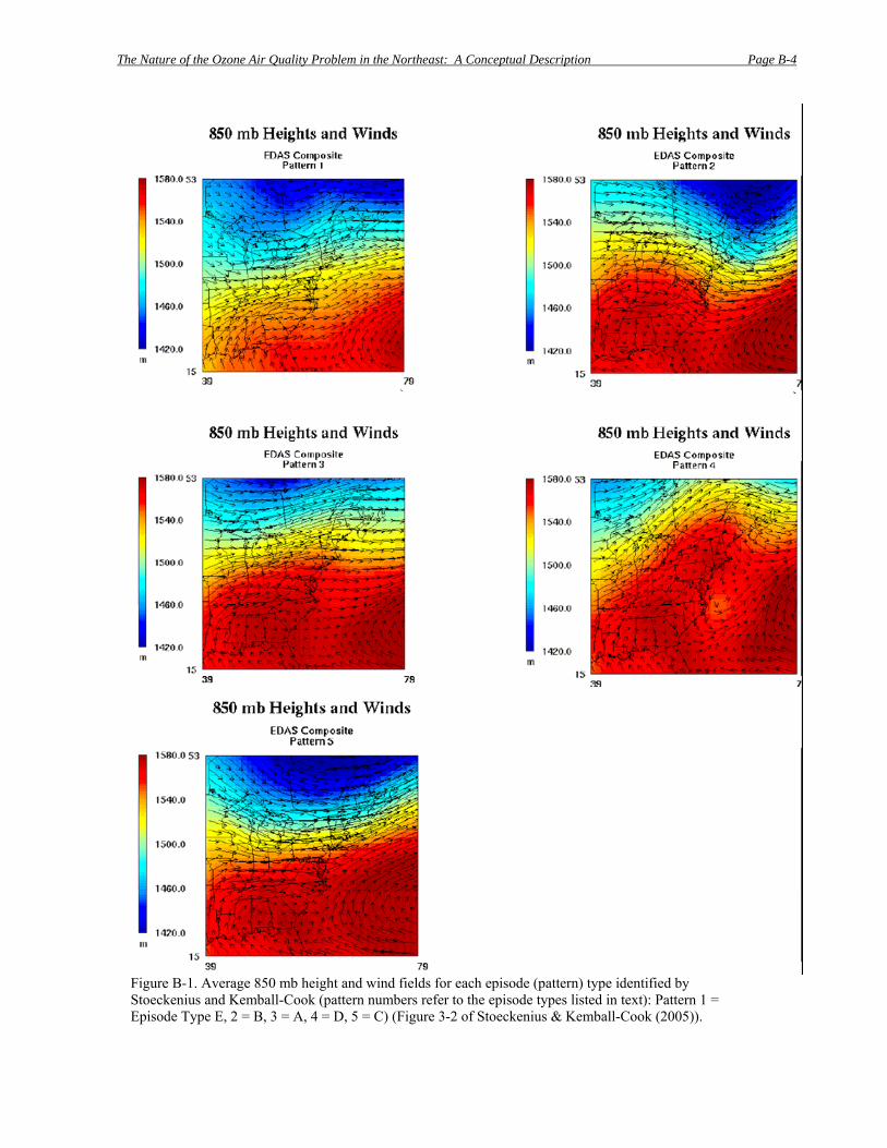
The Nature of the Ozone Air Quality Problem in the Northeast: A Conceptual Description Page B-4
Figure B-1. Average 850 mb height and wind fields for each episode (pattern) type identified by Stoeckenius and Kemball-Cook (pattern numbers refer to the episode types listed in text): Pattern 1 = Episode Type E, 2 = B, 3 = A, 4 = D, 5 = C) (Figure 3-2 of Stoeckenius & Kemball-Cook (2005)).
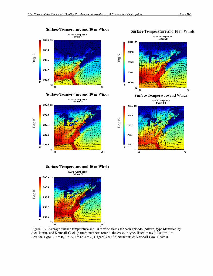
The Nature of the Ozone Air Quality Problem in the Northeast: A Conceptual Description Page B-5
Figure B-2. Average surface temperature and 10 m wind fields for each episode (pattern) type identified by Stoeckenius and Kemball-Cook (pattern numbers refer to the episode types listed in text): Pattern 1 = Episode Type E, 2 = B, 3 = A, 4 = D, 5 = C) (Figure 3-5 of Stoeckenius & Kemball-Cook (2005)).

The Nature of the Ozone Air Quality Problem in the Northeast: A Conceptual Description Page C-1
Appendix C: Exceedance days by monitor in the OTR
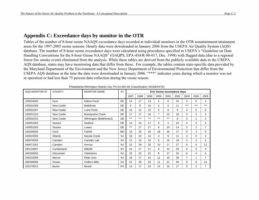
The Nature of the Ozone Air Quality Problem in the Northeast: A Conceptual Description Page C-2
Appendix C: Exceedance days by monitor in the OTR Tables of the number of 8-hour ozone NAAQS exceedance days recorded at individual monitors in the OTR nonattainment/attainment areas for the 1997-2005 ozone seasons. Hourly data were downloaded in January 2006 from the USEPA Air Quality System (AQS) database. The number of 8-hour ozone exceedance days were calculated using procedures specified in USEPA’s “Guideline on Data Handling Conventions for the 8-hour Ozone NAAQS” (OAQPS, EPA-454/R-98-017, Dec. 1998) with flagged data (due to a regional forest fire smoke event) eliminated from the analysis. While these tables are derived from the publicly available data in the USEPA AQS database, states may have monitoring data that differ from these. For example, the tables contain state-specific data provided by the Maryland Department of the Environment and the New Jersey Department of Environmental Protection that differ from the USEPA AQS database at the time the data were downloaded in January 2006. “***” indicates years during which a monitor was not in operation or had less than 75 percent data collection during the ozone season.
Philadelphia-Wilmington-Atlantic City, PA-NJ-MD-DE (Classification: MODERATE)
AQS MONITOR ID COUNTY MONITOR NAME ST 8-hr Ozone exceedance days
1997 1998 1999 2000 2001 2002 2003 2004 2005
100010002 Kent Killens Pond DE 14 17 13 5 8 10 3 0 2
100031003 New Castle Bellefonte DE 6 8 10 5 5 11 *** *** *** 100031007 New Castle Lums Pond DE 15 12 12 5 9 9 4 0 6 100031010 New Castle Brandywine Creek DE 17 17 16 7 15 18 3 3 3 100031013 New Castle Wilmington (Bellefonte2) DE *** *** *** *** *** 8 3 1 4 100051002 Sussex Seaford DE 14 16 17 5 4 10 4 0 3 100051003 Sussex Lewes DE *** 17 17 6 10 14 4 2 7 240150003 Cecil Fairhill MD 19 20 20 18 16 17 6 3 9 340010005 Atlantic Nacote Creek NJ 18 24 14 4 9 11 4 0 3 340070003 Camden Camden Lab NJ 12 15 16 6 19 19 4 3 5 340071001 Camden Ancora NJ 23 29 25 10 17 27 9 6 12 340110007 Cumberland Millville NJ 14 17 17 6 14 20 6 2 4 340150002 Gloucester Clarksboro NJ 19 22 21 8 17 24 6 4 6 340210005 Mercer Rider Univ. NJ 16 17 24 11 15 26 7 1 7 340290006 Ocean Colliers Mills NJ 21 28 23 11 21 30 9 8 14 420170012 Bucks Bristol PA 14 17 24 14 16 17 9 2 7
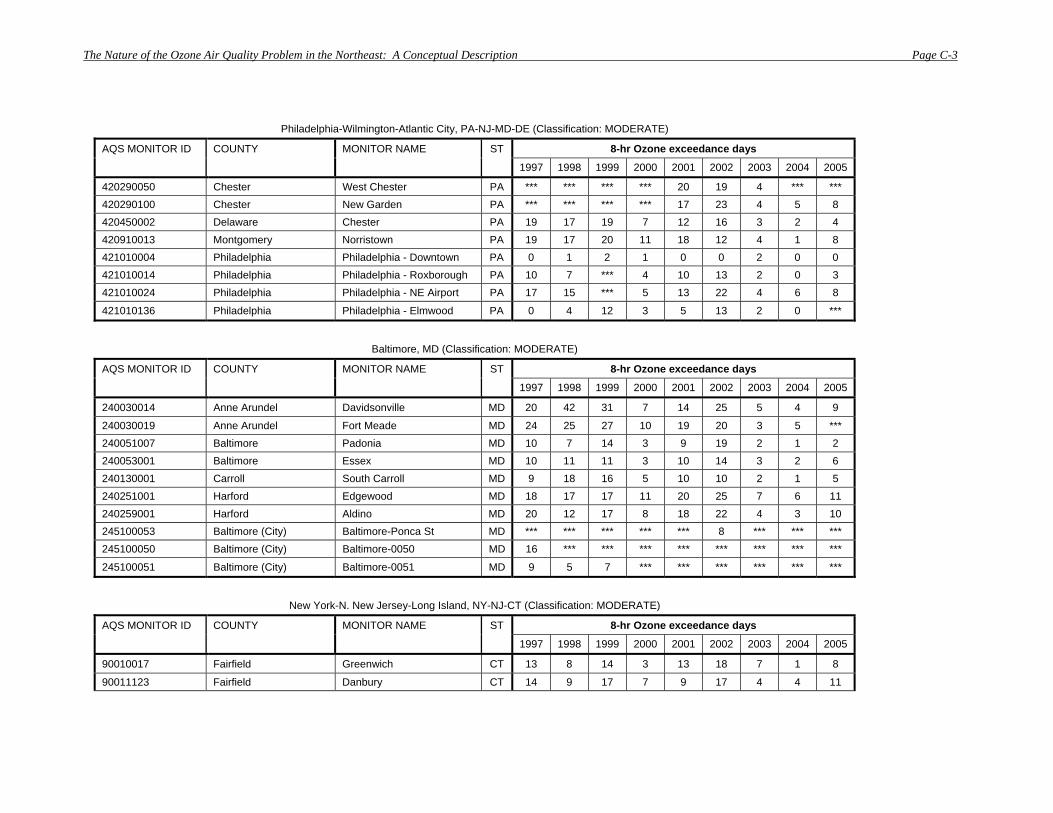
The Nature of the Ozone Air Quality Problem in the Northeast: A Conceptual Description Page C-3
Philadelphia-Wilmington-Atlantic City, PA-NJ-MD-DE (Classification: MODERATE)
AQS MONITOR ID COUNTY MONITOR NAME ST 8-hr Ozone exceedance days
1997 1998 1999 2000 2001 2002 2003 2004 2005
420290050 Chester West Chester PA *** *** *** *** 20 19 4 *** *** 420290100 Chester New Garden PA *** *** *** *** 17 23 4 5 8 420450002 Delaware Chester PA 19 17 19 7 12 16 3 2 4 420910013 Montgomery Norristown PA 19 17 20 11 18 12 4 1 8 421010004 Philadelphia Philadelphia - Downtown PA 0 1 2 1 0 0 2 0 0 421010014 Philadelphia Philadelphia - Roxborough PA 10 7 *** 4 10 13 2 0 3 421010024 Philadelphia Philadelphia - NE Airport PA 17 15 *** 5 13 22 4 6 8
421010136 Philadelphia Philadelphia - Elmwood PA 0 4 12 3 5 13 2 0 ***
Baltimore, MD (Classification: MODERATE)
AQS MONITOR ID COUNTY MONITOR NAME ST 8-hr Ozone exceedance days
1997 1998 1999 2000 2001 2002 2003 2004 2005
240030014 Anne Arundel Davidsonville MD 20 42 31 7 14 25 5 4 9
240030019 Anne Arundel Fort Meade MD 24 25 27 10 19 20 3 5 *** 240051007 Baltimore Padonia MD 10 7 14 3 9 19 2 1 2 240053001 Baltimore Essex MD 10 11 11 3 10 14 3 2 6 240130001 Carroll South Carroll MD 9 18 16 5 10 10 2 1 5 240251001 Harford Edgewood MD 18 17 17 11 20 25 7 6 11 240259001 Harford Aldino MD 20 12 17 8 18 22 4 3 10 245100053 Baltimore (City) Baltimore-Ponca St MD *** *** *** *** *** 8 *** *** *** 245100050 Baltimore (City) Baltimore-0050 MD 16 *** *** *** *** *** *** *** ***
245100051 Baltimore (City) Baltimore-0051 MD 9 5 7 *** *** *** *** *** ***
New York-N. New Jersey-Long Island, NY-NJ-CT (Classification: MODERATE)
AQS MONITOR ID COUNTY MONITOR NAME ST 8-hr Ozone exceedance days
1997 1998 1999 2000 2001 2002 2003 2004 2005
90010017 Fairfield Greenwich CT 13 8 14 3 13 18 7 1 8
90011123 Fairfield Danbury CT 14 9 17 7 9 17 4 4 11
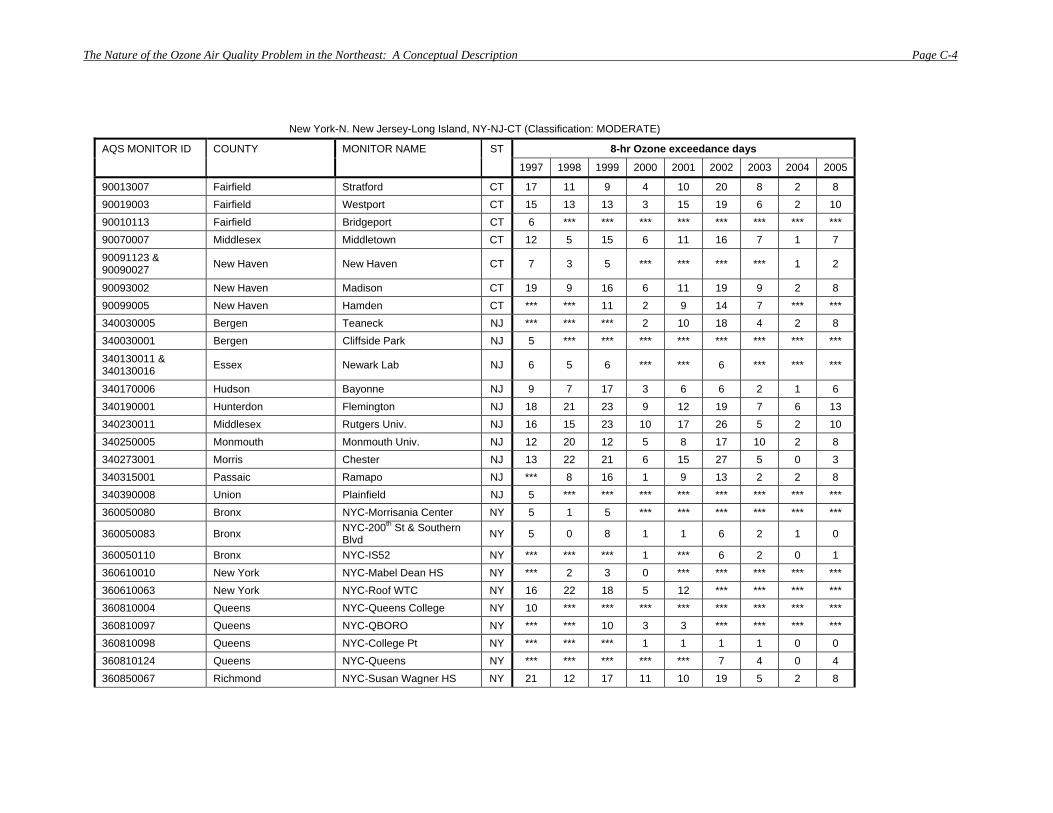
The Nature of the Ozone Air Quality Problem in the Northeast: A Conceptual Description Page C-4
New York-N. New Jersey-Long Island, NY-NJ-CT (Classification: MODERATE)
AQS MONITOR ID COUNTY MONITOR NAME ST 8-hr Ozone exceedance days
1997 1998 1999 2000 2001 2002 2003 2004 2005
90013007 Fairfield Stratford CT 17 11 9 4 10 20 8 2 8 90019003 Fairfield Westport CT 15 13 13 3 15 19 6 2 10 90010113 Fairfield Bridgeport CT 6 *** *** *** *** *** *** *** *** 90070007 Middlesex Middletown CT 12 5 15 6 11 16 7 1 7
90091123 & 90090027 New Haven New Haven CT 7 3 5 *** *** *** *** 1 2
90093002 New Haven Madison CT 19 9 16 6 11 19 9 2 8 90099005 New Haven Hamden CT *** *** 11 2 9 14 7 *** *** 340030005 Bergen Teaneck NJ *** *** *** 2 10 18 4 2 8 340030001 Bergen Cliffside Park NJ 5 *** *** *** *** *** *** *** ***
340130011 & 340130016 Essex Newark Lab NJ 6 5 6 *** *** 6 *** *** ***
340170006 Hudson Bayonne NJ 9 7 17 3 6 6 2 1 6 340190001 Hunterdon Flemington NJ 18 21 23 9 12 19 7 6 13 340230011 Middlesex Rutgers Univ. NJ 16 15 23 10 17 26 5 2 10 340250005 Monmouth Monmouth Univ. NJ 12 20 12 5 8 17 10 2 8 340273001 Morris Chester NJ 13 22 21 6 15 27 5 0 3 340315001 Passaic Ramapo NJ *** 8 16 1 9 13 2 2 8 340390008 Union Plainfield NJ 5 *** *** *** *** *** *** *** *** 360050080 Bronx NYC-Morrisania Center NY 5 1 5 *** *** *** *** *** ***
360050083 Bronx NYC-200th St & Southern Blvd NY 5 0 8 1 1 6 2 1 0
360050110 Bronx NYC-IS52 NY *** *** *** 1 *** 6 2 0 1 360610010 New York NYC-Mabel Dean HS NY *** 2 3 0 *** *** *** *** *** 360610063 New York NYC-Roof WTC NY 16 22 18 5 12 *** *** *** *** 360810004 Queens NYC-Queens College NY 10 *** *** *** *** *** *** *** *** 360810097 Queens NYC-QBORO NY *** *** 10 3 3 *** *** *** *** 360810098 Queens NYC-College Pt NY *** *** *** 1 1 1 1 0 0 360810124 Queens NYC-Queens NY *** *** *** *** *** 7 4 0 4 360850067 Richmond NYC-Susan Wagner HS NY 21 12 17 11 10 19 5 2 8

The Nature of the Ozone Air Quality Problem in the Northeast: A Conceptual Description Page C-5
New York-N. New Jersey-Long Island, NY-NJ-CT (Classification: MODERATE)
AQS MONITOR ID COUNTY MONITOR NAME ST 8-hr Ozone exceedance days
1997 1998 1999 2000 2001 2002 2003 2004 2005
361030002 Suffolk Babylon NY 8 10 11 4 2 9 6 2 6 361030004 Suffolk Riverhead NY 11 9 16 4 3 6 3 *** 6 361030009 Suffolk Holtsville NY *** *** *** 4 8 18 6 2 ***
361192004 Westchester White Plains NY 11 6 12 2 8 15 4 0 9
Washington, DC-MD-VA (Classification: MODERATE)
AQS MONITOR ID COUNTY MONITOR NAME ST 8-hr Ozone exceedance days
1997 1998 1999 2000 2001 2002 2003 2004 2005
110010025 District of Columbia (all) Takoma DC 11 18 15 5 7 13 3 2 1
110010041 District of Columbia (all) River Terrace DC 12 11 16 2 7 12 2 0 1 110010043 District of Columbia (all) McMillian Reservoir DC 18 20 22 2 12 21 3 3 5
240090010 & 240090011 Calvert Calvert MD 4 10 10 5 5 *** *** *** 2
240170010 Charles S. Maryland MD 17 30 31 5 9 15 6 1 6 240210037 Frederick Frederick Municipal Airport MD *** *** 19 4 14 13 3 1 1 240313001 Montgomery Rockville MD 13 22 16 2 11 11 3 2 3 240330002 Prince George's Greenbelt MD 24 24 23 7 19 15 3 *** *** 240338001 Prince George's Suitland MD 14 25 18 3 14 *** *** *** *** 240338003 Prince George's Equestrian Center MD *** *** *** *** *** 15 4 5 5 510130020 Arlington Co Aurora Hills VA 17 10 21 3 12 18 4 4 5 510590005 Fairfax Chantilly (Cub Run) VA 2 16 6 2 9 12 2 3 0 510590018 Fairfax Mount Vernon VA *** 17 16 4 10 16 5 6 8 510590030 Fairfax Franconia VA *** *** 19 0 14 18 5 5 6
510591004 & 510591005 Fairfax Seven Corners &
Annandale VA 10 17 9 2 *** 20 3 4 4
510595001 Fairfax McLean – Lewinsville VA 3 7 6 2 8 7 3 3 2 511071005 Loudoun Ashburn VA *** 17 7 1 9 23 3 2 *** 511530009 Prince William James S. Long Park VA 4 13 9 2 6 7 4 1 0
515100009 Alexandria (City) Alexandria VA 5 10 10 2 6 10 3 3 2
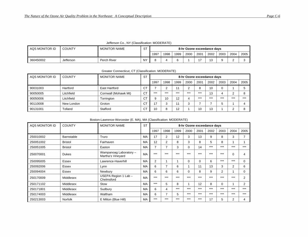
The Nature of the Ozone Air Quality Problem in the Northeast: A Conceptual Description Page C-6
Jefferson Co., NY (Classification: MODERATE)
AQS MONITOR ID COUNTY MONITOR NAME ST 8-hr Ozone exceedance days
1997 1998 1999 2000 2001 2002 2003 2004 2005
360450002 Jefferson Perch River NY 8 4 6 1 17 13 9 2 3
Greater Connecticut, CT (Classification: MODERATE)
AQS MONITOR ID COUNTY MONITOR NAME ST 8-hr Ozone exceedance days
1997 1998 1999 2000 2001 2002 2003 2004 2005
90031003 Hartford East Hartford CT 7 2 11 2 8 10 0 1 5
90050005 Litchfield Cornwall (Mohawk Mt) CT *** *** *** *** *** 13 4 2 8 90050006 Litchfield Torrington CT 9 10 12 4 *** *** *** *** *** 90110008 New London Groton CT 17 3 11 3 7 7 5 1 4
90131001 Tolland Stafford CT 10 8 12 1 10 13 1 2 8
Boston-Lawrence-Worcester (E. MA), MA (Classification: MODERATE)
AQS MONITOR ID COUNTY MONITOR NAME ST 8-hr Ozone exceedance days
1997 1998 1999 2000 2001 2002 2003 2004 2005
250010002 Barnstable Truro MA 17 2 12 3 13 9 8 3 7
250051002 Bristol Fairhaven MA 12 2 8 3 8 5 8 1 1 250051005 Bristol Easton MA 7 7 3 0 14 *** *** *** ***
250070001 Dukes Wampanoag Laboratory – Martha’s Vineyard MA *** *** *** *** *** *** *** 0 4
250095005 Essex Lawrence-Haverhill MA 2 1 1 0 0 6 *** *** 0 250092006 Essex Lynn MA 6 7 6 1 11 13 3 2 6 250094004 Essex Newbury MA 6 6 6 0 8 9 2 1 0
250170009 Middlesex USEPA Region 1 Lab – Chelmsford MA *** *** *** *** *** *** *** *** 2
250171102 Middlesex Stow MA *** 5 8 1 12 8 0 1 2 250171801 Middlesex Sudbury MA 6 4 *** *** *** *** *** *** *** 250174003 Middlesex Waltham MA 6 7 5 *** *** *** *** *** *** 250213003 Norfolk E Milton (Blue Hill) MA *** *** *** *** *** 17 5 2 4
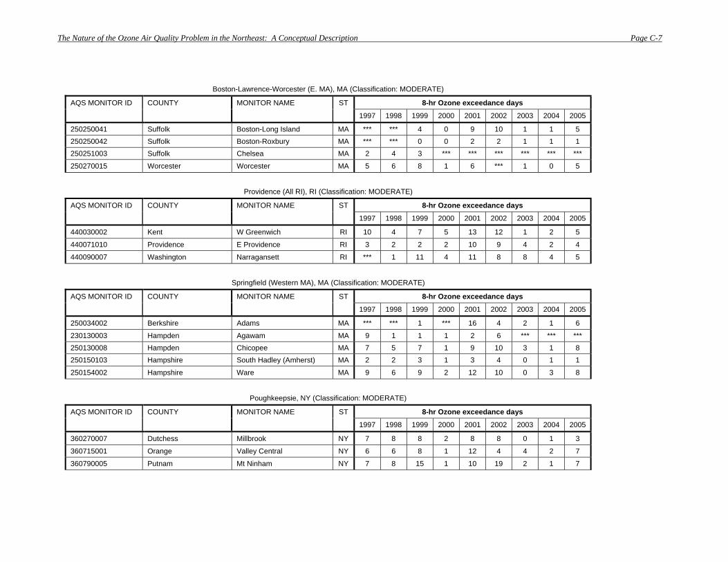
The Nature of the Ozone Air Quality Problem in the Northeast: A Conceptual Description Page C-7
Boston-Lawrence-Worcester (E. MA), MA (Classification: MODERATE)
AQS MONITOR ID COUNTY MONITOR NAME ST 8-hr Ozone exceedance days
1997 1998 1999 2000 2001 2002 2003 2004 2005
250250041 Suffolk Boston-Long Island MA *** *** 4 0 9 10 1 1 5 250250042 Suffolk Boston-Roxbury MA *** *** 0 0 2 2 1 1 1 250251003 Suffolk Chelsea MA 2 4 3 *** *** *** *** *** ***
250270015 Worcester Worcester MA 5 6 8 1 6 *** 1 0 5
Providence (All RI), RI (Classification: MODERATE)
AQS MONITOR ID COUNTY MONITOR NAME ST 8-hr Ozone exceedance days
1997 1998 1999 2000 2001 2002 2003 2004 2005
440030002 Kent W Greenwich RI 10 4 7 5 13 12 1 2 5
440071010 Providence E Providence RI 3 2 2 2 10 9 4 2 4
440090007 Washington Narragansett RI *** 1 11 4 11 8 8 4 5
Springfield (Western MA), MA (Classification: MODERATE)
AQS MONITOR ID COUNTY MONITOR NAME ST 8-hr Ozone exceedance days
1997 1998 1999 2000 2001 2002 2003 2004 2005
250034002 Berkshire Adams MA *** *** 1 *** 16 4 2 1 6
230130003 Hampden Agawam MA 9 1 1 1 2 6 *** *** *** 250130008 Hampden Chicopee MA 7 5 7 1 9 10 3 1 8 250150103 Hampshire South Hadley (Amherst) MA 2 2 3 1 3 4 0 1 1
250154002 Hampshire Ware MA 9 6 9 2 12 10 0 3 8
Poughkeepsie, NY (Classification: MODERATE)
AQS MONITOR ID COUNTY MONITOR NAME ST 8-hr Ozone exceedance days
1997 1998 1999 2000 2001 2002 2003 2004 2005
360270007 Dutchess Millbrook NY 7 8 8 2 8 8 0 1 3
360715001 Orange Valley Central NY 6 6 8 1 12 4 4 2 7
360790005 Putnam Mt Ninham NY 7 8 15 1 10 19 2 1 7

The Nature of the Ozone Air Quality Problem in the Northeast: A Conceptual Description Page C-8
Boston-Manchester-Portsmouth (SE), NH (Classification: MODERATE)
AQS MONITOR ID COUNTY MONITOR NAME ST 8-hr Ozone exceedance days
1997 1998 1999 2000 2001 2002 2003 2004 2005
330110016 & 330110019 & 330110020
Hillsborough Manchester NH 3 0 *** 0 *** 4 0 1 0
330111010 & 330111011 Hillsborough Nashua NH 4 3 8 1 7 5 1 2 1
330150009 & 330150015 & 330150014
Rockingham Portsmouth NH 5 3 5 0 *** 8 0 1 0
330150013 Rockingham Brentwood NH *** 0 1 0 4 10 *** *** ***
330150012 & 330150016 Rockingham Rye NH 9 4 3 0 7 7 0 1 0
330173002 Strafford Rochester NH 1 0 2 0 1 6 0 *** ***
Kent and Queen Anne’s Cos., MD (Classification: MARGINAL)
AQS MONITOR ID COUNTY MONITOR NAME ST 8-hr Ozone exceedance days
1997 1998 1999 2000 2001 2002 2003 2004 2005
240290002 Kent Millington MD 19 16 22 6 13 17 4 1 3
Lancaster, PA (Classification: MARGINAL)
AQS MONITOR ID COUNTY MONITOR NAME ST 8-hr Ozone exceedance days
1997 1998 1999 2000 2001 2002 2003 2004 2005
420710007 Lancaster Lancaster PA 21 27 18 5 15 18 3 1 6

The Nature of the Ozone Air Quality Problem in the Northeast: A Conceptual Description Page C-9
Portland, ME (Classification: MARGINAL)
AQS MONITOR ID COUNTY MONITOR NAME ST 8-hr Ozone exceedance days
1997 1998 1999 2000 2001 2002 2003 2004 2005
230050027 Cumberland Portland ME *** *** *** *** *** *** *** 0 0
230052003 Cumberland Cape Elizabeth ME 6 5 2 0 8 5 0 0 0
230230003 & 230230004 Sagadahoc Phippsburg/Georgetown
(Reid State Park) ME 7 4 4 1 *** 5 1 0 0
230313002 York Kittery ME 7 4 4 0 4 12 2 1 0 230312002 York Kennebunkport ME 5 5 5 1 8 10 2 1 0
230310037 & 230310038 York Hollis ME 2 0 1 0 *** 3 0 0 0
Buffalo-Niagara Falls, NY (Classification: SUBPART 1)
AQS MONITOR ID COUNTY MONITOR NAME ST 8-hr Ozone exceedance days
1997 1998 1999 2000 2001 2002 2003 2004 2005
360290002 Erie Amherst NY 0 13 6 4 10 21 7 0 5
360631006 Niagara Middleport NY 1 6 7 3 10 16 6 0 4
Youngstown-Warren-Sharon, OH-PA (Classification: SUBPART 1)
AQS MONITOR ID COUNTY MONITOR NAME ST 8-hr Ozone exceedance days
1997 1998 1999 2000 2001 2002 2003 2004 2005
390990009 & 390990013 Mahoning Youngstown - Oakhill OH 3 15 7 1 5 14 4 1 2
391550008 & 391550011 Trumbull Warren-Trumbull County OH 8 19 10 2 12 24 5 2 5
391550009 Trumbull Kinsman OH 7 15 10 2 5 16 4 0 2
420850100 Mercer Farrell PA 9 24 8 2 15 20 6 1 4

The Nature of the Ozone Air Quality Problem in the Northeast: A Conceptual Description Page C-10
Pittsburgh-Beaver Valley, PA (Classification: SUBPART 1)
AQS MONITOR ID COUNTY MONITOR NAME ST 8-hr Ozone exceedance days
1997 1998 1999 2000 2001 2002 2003 2004 2005
420030008 Allegheny Lawrenceville PA 7 14 10 3 4 16 5 0 1
420030010 Allegheny Pittsburg PA *** 6 16 4 9 25 5 0 4 420030067 Allegheny South Fayette PA 8 24 15 4 7 17 4 1 4 420030088 Allegheny Penn Hills PA 5 16 11 4 *** *** *** *** *** 420031005 Allegheny Harrison Township PA 12 18 14 4 8 14 2 0 6 420050001 Armstrong Kittanning PA *** 21 18 2 16 15 5 1 4 420070002 Beaver Hookstown PA 4 11 9 1 9 19 6 0 5 420070005 Beaver Brighton Township PA 3 15 11 1 8 23 3 0 4 420070014 Beaver Beaver Falls PA 5 10 6 3 4 9 3 0 2 421250005 Washington Charleroi PA 14 34 11 3 7 14 4 0 2 421250200 Washington Washington PA 6 15 11 3 6 9 5 0 4 421255001 Washington Florence PA 4 11 9 2 7 17 3 0 4 421290006 Westmoreland Murrysville PA 4 3 5 2 1 9 2 0 4
421290008 Westmoreland Greensburg PA *** *** 16 3 3 10 4 0 2
Jamestown, NY (Classification: SUBPART 1)
AQS MONITOR ID COUNTY MONITOR NAME ST 8-hr Ozone exceedance days
1997 1998 1999 2000 2001 2002 2003 2004 2005
360130006 Chautauqua Dunkirk NY *** *** 12 5 11 23 7 4 6
360130011 Chautauqua Westfield NY 4 11 8 3 4 18 4 0 2
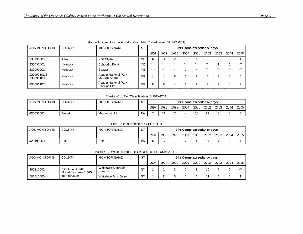
The Nature of the Ozone Air Quality Problem in the Northeast: A Conceptual Description Page C-11
Hancock, Knox, Lincoln & Waldo Cos., ME (Classification: SUBPART 1)
AQS MONITOR ID COUNTY MONITOR NAME ST 8-hr Ozone exceedance days
1997 1998 1999 2000 2001 2002 2003 2004 2005
230130004 Knox Port Clyde ME 6 3 2 0 6 5 3 0 1
230090401 Hancock Schoodic Point ME *** *** *** *** *** *** 1 0 *** 230090001 Hancock Seawall ME *** *** *** 0 4 *** *** *** ***
230090101 & 230090103 Hancock Acadia National Park –
McFarland Hill ME 1 4 5 0 9 6 2 0 0
230090102 Hancock Acadia National Park – Cadillac Mtn. ME 5 8 4 3 9 8 3 0 3
Franklin Co., PA (Classification: SUBPART 1)
AQS MONITOR ID COUNTY MONITOR NAME ST 8-hr Ozone exceedance days
1997 1998 1999 2000 2001 2002 2003 2004 2005
420550001 Franklin Methodist Hill PA 7 22 20 4 15 27 3 0 0
Erie, PA (Classification: SUBPART 1)
AQS MONITOR ID COUNTY MONITOR NAME ST 8-hr Ozone exceedance days
1997 1998 1999 2000 2001 2002 2003 2004 2005
420490003 Erie Erie PA 6 12 13 2 4 17 4 0 4
Essex Co. (Whiteface Mtn.), NY (Classification: SUBPART 1)
AQS MONITOR ID COUNTY MONITOR NAME ST 8-hr Ozone exceedance days
1997 1998 1999 2000 2001 2002 2003 2004 2005
360310002 Whiteface Mountain Summit NY 2 1 3 2 5 12 7 0 ***
360310003
Essex (Whiteface Mountain above 1,900 foot elevation ) Whiteface Mtn. Base NY 1 2 3 0 3 11 5 0 1

The Nature of the Ozone Air Quality Problem in the Northeast: A Conceptual Description Page C-12
Allentown-Bethlehem-Easton, PA (Classification: SUBPART 1)
AQS MONITOR ID COUNTY MONITOR NAME ST 8-hr Ozone exceedance days
1997 1998 1999 2000 2001 2002 2003 2004 2005
420770004 Lehigh Allentown PA 12 18 19 5 9 16 4 3 6
420950025 Northampton Freemansburg PA 0 5 22 6 14 12 4 6 5
420950100 & 420958000 Northampton Easton PA 11 8 12 2 11 13 3 1 1
Reading, PA (Classification: SUBPART 1)
AQS MONITOR ID COUNTY MONITOR NAME ST 8-hr Ozone exceedance days
1997 1998 1999 2000 2001 2002 2003 2004 2005
420110001 Berks Kutztown PA 6 14 12 2 7 11 1 *** ***
420110009 & 420110010 Berks Reading PA 10 16 14 3 8 13 3 1 4
Clearfield and Indiana Cos., PA (Classification: SUBPART 1)
AQS MONITOR ID COUNTY MONITOR NAME ST 8-hr Ozone exceedance days
1997 1998 1999 2000 2001 2002 2003 2004 2005
420630004 Indiana Strongstown PA *** *** *** *** *** *** *** *** 5
420334000 Clearfield Moshannon PA 12 16 1 2 8 13 4 0 4
Greene Co., PA (Classification: SUBPART 1)
AQS MONITOR ID COUNTY MONITOR NAME ST 8-hr Ozone exceedance days
1997 1998 1999 2000 2001 2002 2003 2004 2005
420590002 Greene Holbrook PA *** *** 21 6 12 9 3 0 5
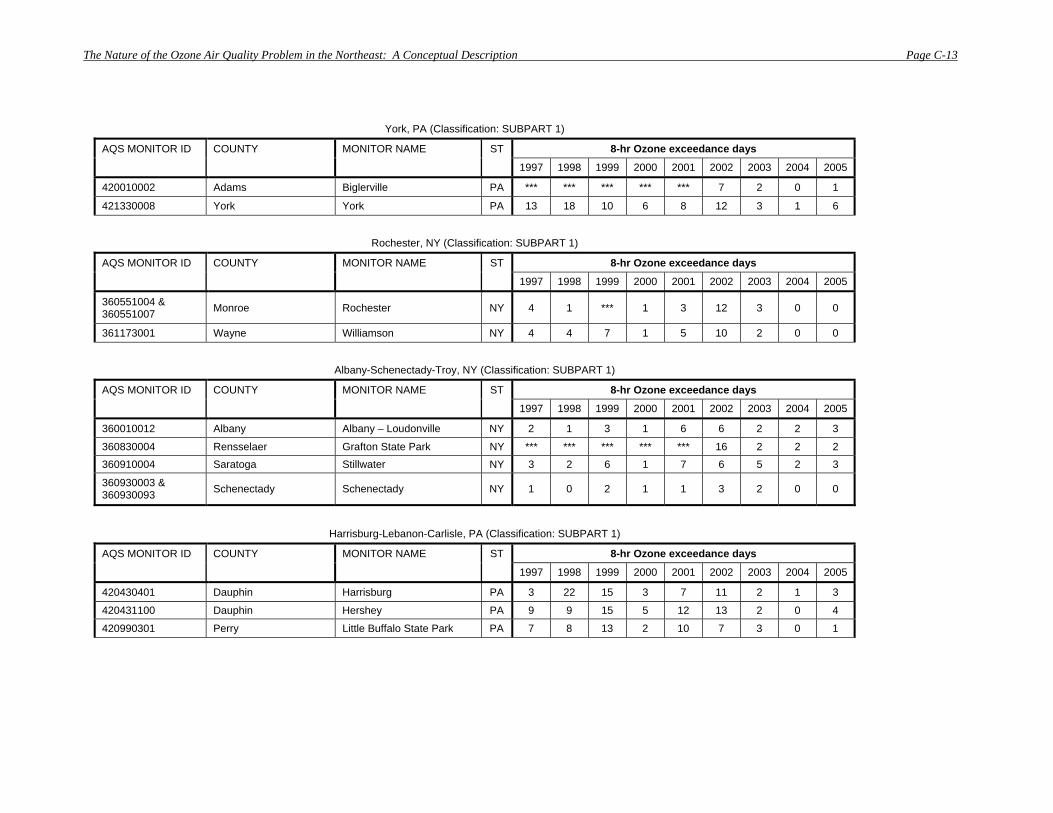
The Nature of the Ozone Air Quality Problem in the Northeast: A Conceptual Description Page C-13
York, PA (Classification: SUBPART 1)
AQS MONITOR ID COUNTY MONITOR NAME ST 8-hr Ozone exceedance days
1997 1998 1999 2000 2001 2002 2003 2004 2005
420010002 Adams Biglerville PA *** *** *** *** *** 7 2 0 1
421330008 York York PA 13 18 10 6 8 12 3 1 6
Rochester, NY (Classification: SUBPART 1)
AQS MONITOR ID COUNTY MONITOR NAME ST 8-hr Ozone exceedance days
1997 1998 1999 2000 2001 2002 2003 2004 2005
360551004 & 360551007 Monroe Rochester NY 4 1 *** 1 3 12 3 0 0
361173001 Wayne Williamson NY 4 4 7 1 5 10 2 0 0
Albany-Schenectady-Troy, NY (Classification: SUBPART 1)
AQS MONITOR ID COUNTY MONITOR NAME ST 8-hr Ozone exceedance days
1997 1998 1999 2000 2001 2002 2003 2004 2005
360010012 Albany Albany – Loudonville NY 2 1 3 1 6 6 2 2 3
360830004 Rensselaer Grafton State Park NY *** *** *** *** *** 16 2 2 2 360910004 Saratoga Stillwater NY 3 2 6 1 7 6 5 2 3
360930003 & 360930093 Schenectady Schenectady NY 1 0 2 1 1 3 2 0 0
Harrisburg-Lebanon-Carlisle, PA (Classification: SUBPART 1)
AQS MONITOR ID COUNTY MONITOR NAME ST 8-hr Ozone exceedance days
1997 1998 1999 2000 2001 2002 2003 2004 2005
420430401 Dauphin Harrisburg PA 3 22 15 3 7 11 2 1 3
420431100 Dauphin Hershey PA 9 9 15 5 12 13 2 0 4
420990301 Perry Little Buffalo State Park PA 7 8 13 2 10 7 3 0 1

The Nature of the Ozone Air Quality Problem in the Northeast: A Conceptual Description Page C-14
Johnstown, PA (Classification: SUBPART 1)
AQS MONITOR ID COUNTY MONITOR NAME ST 8-hr Ozone exceedance days
1997 1998 1999 2000 2001 2002 2003 2004 2005
420210011 Cambria Johnstown PA 7 13 11 5 5 6 2 0 1
Scranton-Wilkes-Barre, PA (Classification: SUBPART 1)
AQS MONITOR ID COUNTY MONITOR NAME ST 8-hr Ozone exceedance days
1997 1998 1999 2000 2001 2002 2003 2004 2005
420690101 Lackawanna Peckville PA 6 5 11 1 5 14 2 0 2
420692006 Lackawanna Scranton PA 4 5 11 1 5 8 2 0 1 420791100 Luzerne Nanticoke PA 0 2 4 1 5 6 3 0 0 420791101 Luzerne Wilkes-Barre PA 8 7 9 1 7 7 2 0 1
State College, PA (Classification: SUBPART 1)
AQS MONITOR ID COUNTY MONITOR NAME ST 8-hr Ozone exceedance days
1997 1998 1999 2000 2001 2002 2003 2004 2005
420270100 Centre State College PA *** *** *** 2 5 8 3 0 1
420274000 Centre Penn Nursery PA 7 8 4 2 1 12 4 0 ***
Tioga Co., PA (Classification: SUBPART 1)
AQS MONITOR ID COUNTY MONITOR NAME ST 8-hr Ozone exceedance days
1997 1998 1999 2000 2001 2002 2003 2004 2005
421174000 Tioga Tioga PA *** *** *** 2 3 8 3 0 0
Altoona, PA (Classification: SUBPART 1)
AQS MONITOR ID COUNTY MONITOR NAME ST 8-hr Ozone exceedance days
1997 1998 1999 2000 2001 2002 2003 2004 2005
420130801 Blair Altoona PA 7 17 6 2 3 9 3 0 1
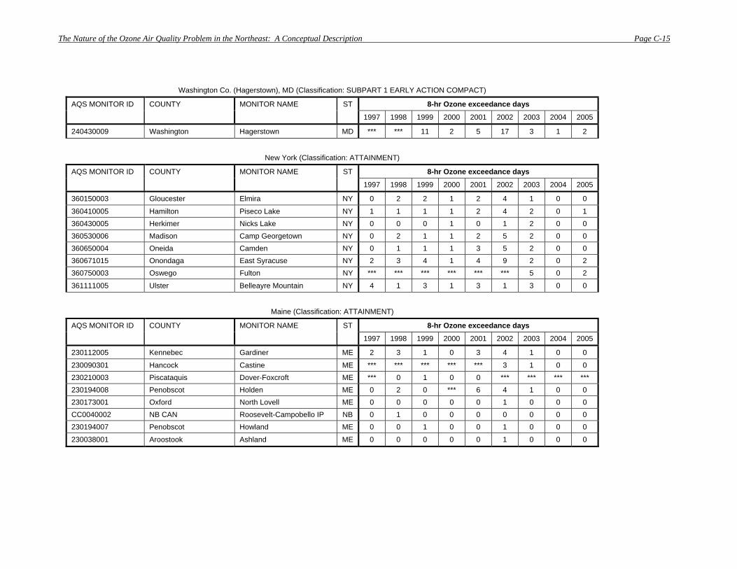
The Nature of the Ozone Air Quality Problem in the Northeast: A Conceptual Description Page C-15
Washington Co. (Hagerstown), MD (Classification: SUBPART 1 EARLY ACTION COMPACT)
AQS MONITOR ID COUNTY MONITOR NAME ST 8-hr Ozone exceedance days
1997 1998 1999 2000 2001 2002 2003 2004 2005
240430009 Washington Hagerstown MD *** *** 11 2 5 17 3 1 2
New York (Classification: ATTAINMENT)
AQS MONITOR ID COUNTY MONITOR NAME ST 8-hr Ozone exceedance days
1997 1998 1999 2000 2001 2002 2003 2004 2005
360150003 Gloucester Elmira NY 0 2 2 1 2 4 1 0 0
360410005 Hamilton Piseco Lake NY 1 1 1 1 2 4 2 0 1 360430005 Herkimer Nicks Lake NY 0 0 0 1 0 1 2 0 0 360530006 Madison Camp Georgetown NY 0 2 1 1 2 5 2 0 0 360650004 Oneida Camden NY 0 1 1 1 3 5 2 0 0 360671015 Onondaga East Syracuse NY 2 3 4 1 4 9 2 0 2 360750003 Oswego Fulton NY *** *** *** *** *** *** 5 0 2
361111005 Ulster Belleayre Mountain NY 4 1 3 1 3 1 3 0 0
Maine (Classification: ATTAINMENT)
AQS MONITOR ID COUNTY MONITOR NAME ST 8-hr Ozone exceedance days
1997 1998 1999 2000 2001 2002 2003 2004 2005
230112005 Kennebec Gardiner ME 2 3 1 0 3 4 1 0 0
230090301 Hancock Castine ME *** *** *** *** *** 3 1 0 0 230210003 Piscataquis Dover-Foxcroft ME *** 0 1 0 0 *** *** *** *** 230194008 Penobscot Holden ME 0 2 0 *** 6 4 1 0 0 230173001 Oxford North Lovell ME 0 0 0 0 0 1 0 0 0 CC0040002 NB CAN Roosevelt-Campobello IP NB 0 1 0 0 0 0 0 0 0 230194007 Penobscot Howland ME 0 0 1 0 0 1 0 0 0
230038001 Aroostook Ashland ME 0 0 0 0 0 1 0 0 0
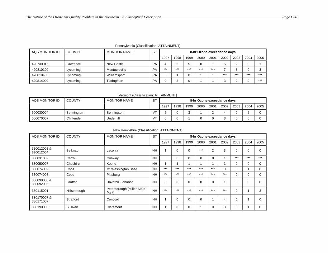
The Nature of the Ozone Air Quality Problem in the Northeast: A Conceptual Description Page C-16
Pennsylvania (Classification: ATTAINMENT)
AQS MONITOR ID COUNTY MONITOR NAME ST 8-hr Ozone exceedance days
1997 1998 1999 2000 2001 2002 2003 2004 2005
420730015 Lawrence New Castle PA 4 2 5 0 1 6 2 0 1
420810100 Lycoming Montoursville PA *** *** *** *** *** 7 3 0 3 420810403 Lycoming Williamsport PA 0 1 0 1 1 *** *** *** ***
420814000 Lycoming Tiadaghton PA 0 3 0 1 1 3 2 0 ***
Vermont (Classification: ATTAINMENT) AQS MONITOR ID COUNTY MONITOR NAME ST 8-hr Ozone exceedance days
1997 1998 1999 2000 2001 2002 2003 2004 2005
500030004 Bennington Bennington VT 2 0 3 1 2 4 0 2 0
500070007 Chittenden Underhill VT 0 0 1 0 0 3 0 0 0
New Hampshire (Classification: ATTAINMENT)
AQS MONITOR ID COUNTY MONITOR NAME ST 8-hr Ozone exceedance days
1997 1998 1999 2000 2001 2002 2003 2004 2005
330012003 & 330012004 Belknap Laconia NH 1 0 0 *** 2 3 0 0 0
330031002 Carroll Conway NH 0 0 0 0 0 1 *** *** *** 330050007 Cheshire Keene NH 1 1 1 1 1 1 0 0 0 330074002 Coos Mt Washington Base NH *** *** *** *** *** 0 0 1 0 330074003 Coos Pittsburg NH *** *** *** *** *** *** 0 0 0
330090008 & 330092005 Grafton Haverhill-Lebanon NH 0 0 0 0 0 1 0 0 0
330115001 Hillsborough Peterborough (Miller State Park) NH *** *** *** *** *** *** 0 1 3
330170007 & 330171007 Strafford Concord NH 1 0 0 0 1 4 0 1 0
330190003 Sullivan Claremont NH 1 0 0 1 0 3 0 1 0

DRAFT – The Nature of the Ozone Air Quality Problem in the Northeast: A Conceptual Description Page D-1
Appendix D: 8-hour ozone design values in the OTR, 1997-2005

DRAFT – The Nature of the Ozone Air Quality Problem in the Northeast: A Conceptual Description Page D-2
Appendix D: 8-hour ozone design values in the OTR, 1997-2005 Tables of the valid 8-hour ozone design values (3-year averages of the ozone season 4th maximum 8-hour ozone concentrations) recorded at individual monitors in OTR nonattainment/attainment areas for the 1997-2005 ozone seasons. Hourly data were downloaded from the USEPA Air Quality System (AQS) database in January 2006. The 8-hour averages and design values were calculated using procedures specified in EPA’s “Guideline on Data Handling Conventions for the 8-hour Ozone NAAQS” (OAQPS, EPA-454/R-98-017, Dec. 1998) with flagged data (due to a regional forest fire smoke event) eliminated from the analysis. “***” indicates years during which a monitor was not in operation or had less than 90 percent data collection (with a design value less than 85 ppb) for the respective 3-year period. Red shading indicates averages ≥ 85 ppb (violating the 8-hr ozone NAAQS), orange shading indicates averages between 80 and 84 ppb, yellow shading indicates average between 75 and 79 ppb and green shading indicates averages < 75 ppb. While these tables are derived from the publicly available data downloaded in January 2006 from the USEPA AQS database, states may have monitoring data that differ from these. For example, design values for New Jersey were provided by the New Jersey Department of Environmental Protection and differ in some instances from the derived values based on the USEPA AQS database.
Philadelphia-Wilmington-Atlantic City, PA-NJ-MD-DE (Classification: MODERATE) 8-hr Ozone DESIGN VALUE (ppb)
AQS MONITOR ID COUNTY MONITOR NAME ST 1997-1999
1998-2000
1999-2001
2000-2002
2001-2003
2002-2004
2003-2005
100010002 Kent Killens Pond DE 99 97 93 92 89 84 80
100031003 New Castle Bellefonte DE 90 91 91 92 *** *** *** 100031007 New Castle Lums Pond DE 100 97 97 96 93 84 80 100031010 New Castle Brandywine Creek DE 99 96 95 96 93 89 82 100031013 New Castle Wilmington (Bellefonte2) DE *** *** *** *** 90 85 82 100051002 Sussex Seaford DE 99 98 95 94 91 85 82 100051003 Sussex Lewes DE *** 95 90 87 88 85 84 240150003 Cecil Fairhill MD 110 106 106 104 98 91 89 340010005 Atlantic Nacote Creek NJ 101 94 95 91 91 85 82 340070003 Camden Camden Lab NJ 104 101 104 101 102 93 85 340071001 Camden Ancora NJ 111 106 108 104 102 96 92 340110007 Cumberland Millville NJ 104 101 102 98 98 91 86 340150002 Gloucester Clarksboro NJ 106 105 105 104 100 94 88 340210005 Mercer Rider Univ. NJ 112 109 112 102 99 91 85
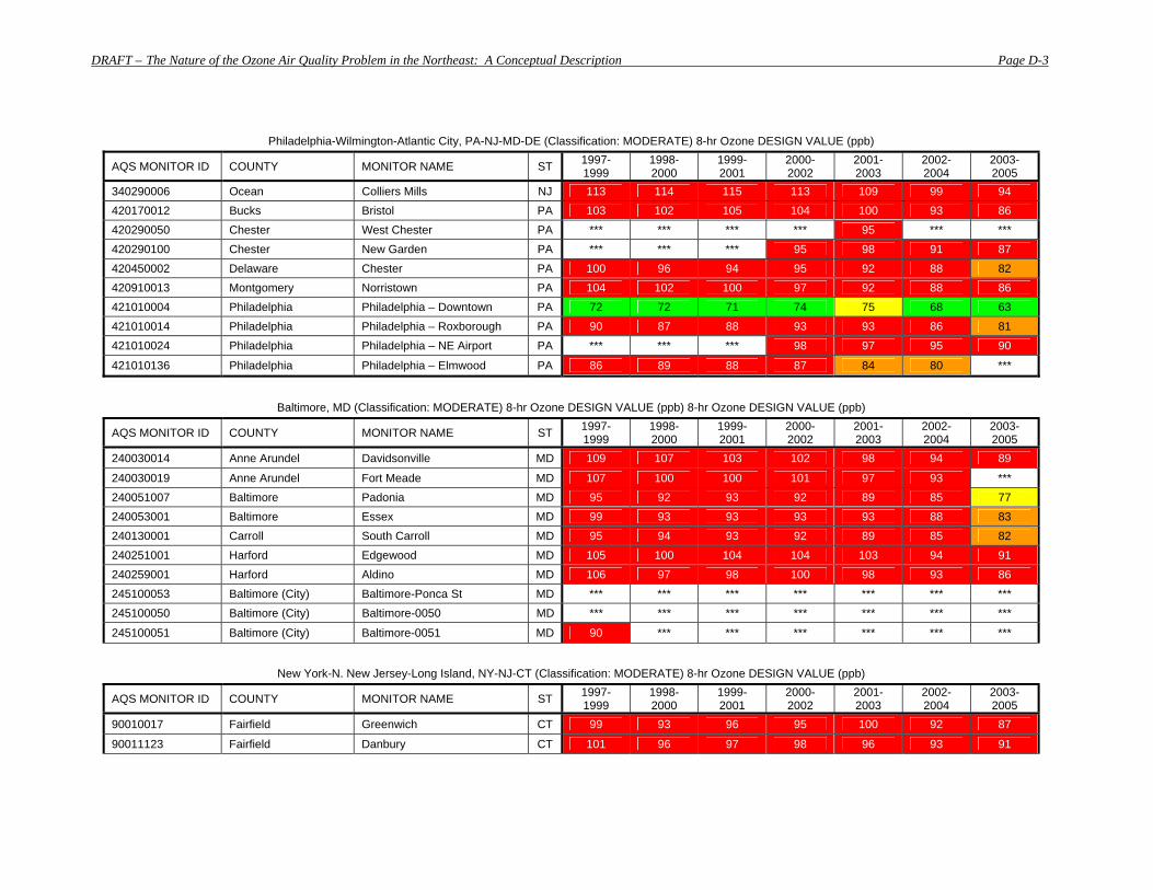
DRAFT – The Nature of the Ozone Air Quality Problem in the Northeast: A Conceptual Description Page D-3
Philadelphia-Wilmington-Atlantic City, PA-NJ-MD-DE (Classification: MODERATE) 8-hr Ozone DESIGN VALUE (ppb)
AQS MONITOR ID COUNTY MONITOR NAME ST 1997-1999
1998-2000
1999-2001
2000-2002
2001-2003
2002-2004
2003-2005
340290006 Ocean Colliers Mills NJ 113 114 115 113 109 99 94 420170012 Bucks Bristol PA 103 102 105 104 100 93 86 420290050 Chester West Chester PA *** *** *** *** 95 *** *** 420290100 Chester New Garden PA *** *** *** 95 98 91 87 420450002 Delaware Chester PA 100 96 94 95 92 88 82 420910013 Montgomery Norristown PA 104 102 100 97 92 88 86 421010004 Philadelphia Philadelphia – Downtown PA 72 72 71 74 75 68 63 421010014 Philadelphia Philadelphia – Roxborough PA 90 87 88 93 93 86 81 421010024 Philadelphia Philadelphia – NE Airport PA *** *** *** 98 97 95 90
421010136 Philadelphia Philadelphia – Elmwood PA 86 89 88 87 84 80 ***
Baltimore, MD (Classification: MODERATE) 8-hr Ozone DESIGN VALUE (ppb) 8-hr Ozone DESIGN VALUE (ppb)
AQS MONITOR ID COUNTY MONITOR NAME ST 1997-1999
1998-2000
1999-2001
2000-2002
2001-2003
2002-2004
2003-2005
240030014 Anne Arundel Davidsonville MD 109 107 103 102 98 94 89
240030019 Anne Arundel Fort Meade MD 107 100 100 101 97 93 *** 240051007 Baltimore Padonia MD 95 92 93 92 89 85 77 240053001 Baltimore Essex MD 99 93 93 93 93 88 83 240130001 Carroll South Carroll MD 95 94 93 92 89 85 82 240251001 Harford Edgewood MD 105 100 104 104 103 94 91 240259001 Harford Aldino MD 106 97 98 100 98 93 86 245100053 Baltimore (City) Baltimore-Ponca St MD *** *** *** *** *** *** *** 245100050 Baltimore (City) Baltimore-0050 MD *** *** *** *** *** *** ***
245100051 Baltimore (City) Baltimore-0051 MD 90 *** *** *** *** *** ***
New York-N. New Jersey-Long Island, NY-NJ-CT (Classification: MODERATE) 8-hr Ozone DESIGN VALUE (ppb)
AQS MONITOR ID COUNTY MONITOR NAME ST 1997-1999
1998-2000
1999-2001
2000-2002
2001-2003
2002-2004
2003-2005
90010017 Fairfield Greenwich CT 99 93 96 95 100 92 87
90011123 Fairfield Danbury CT 101 96 97 98 96 93 91

DRAFT – The Nature of the Ozone Air Quality Problem in the Northeast: A Conceptual Description Page D-4
New York-N. New Jersey-Long Island, NY-NJ-CT (Classification: MODERATE) 8-hr Ozone DESIGN VALUE (ppb)
AQS MONITOR ID COUNTY MONITOR NAME ST 1997-1999
1998-2000
1999-2001
2000-2002
2001-2003
2002-2004
2003-2005
90013007 Fairfield Stratford CT 98 94 96 98 102 95 90 90019003 Fairfield Westport CT 103 94 97 93 97 92 89 90010113 Fairfield Bridgeport CT *** *** *** *** *** *** *** 90070007 Middlesex Middletown CT 99 95 99 97 98 92 90
90091123 & 90090027 New Haven New Haven CT 86 *** *** *** *** *** ***
90093002 New Haven Madison CT 103 96 97 98 102 95 90 90099005 New Haven Hamden CT *** *** 95 94 98 *** *** 340030005 Bergen Teaneck NJ *** *** *** 92 95 89 86 340030001 Bergen Cliffside Park NJ *** *** *** *** *** *** ***
340130011 & 340130016 Essex Newark Lab NJ 93 *** *** *** *** *** ***
340170006 Hudson Bayonne NJ 107 99 100 86 87 82 84 340190001 Hunterdon Flemington NJ 106 103 104 97 97 92 90 340230011 Middlesex Rutgers Univ. NJ 113 109 111 101 98 89 86 340250005 Monmouth Monmouth Univ. NJ 100 102 101 97 97 93 89 340273001 Morris Chester NJ 102 100 101 98 98 90 82 340315001 Passaic Ramapo NJ *** 89 94 88 88 84 81 340390008 Union Plainfield NJ *** *** *** *** *** *** *** 360050080 Bronx NYC-Morrisania Center NY 84 *** *** *** *** *** *** 360050083 Bronx NYC-200th St & Southern Blvd NY 88 80 83 81 84 83 75 360050110 Bronx NYC-IS52 NY *** *** *** *** *** 80 76 360610010 New York NYC-Mabel Dean HS NY *** 69 *** *** *** *** *** 360610063 New York NYC-Roof WTC NY 106 98 98 *** *** *** *** 360810004 Queens NYC-Queens College NY *** *** *** *** *** *** *** 360810097 Queens NYC-QBORO NY *** 88 86 *** *** *** *** 360810098 Queens NYC-College Pt NY *** *** 68 74 75 72 69 360810124 Queens NYC-Queens NY *** *** *** *** *** *** *** 360850067 Richmond NYC-Susan Wagner HS NY 105 96 98 96 94 89 87 361030002 Suffolk Babylon NY 97 91 87 92 95 94 91
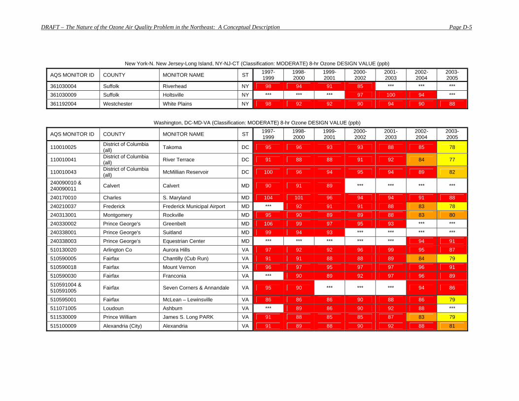
DRAFT – The Nature of the Ozone Air Quality Problem in the Northeast: A Conceptual Description Page D-5
New York-N. New Jersey-Long Island, NY-NJ-CT (Classification: MODERATE) 8-hr Ozone DESIGN VALUE (ppb)
AQS MONITOR ID COUNTY MONITOR NAME ST 1997-1999
1998-2000
1999-2001
2000-2002
2001-2003
2002-2004
2003-2005
361030004 Suffolk Riverhead NY 98 94 91 85 *** *** *** 361030009 Suffolk Holtsville NY *** *** *** 97 100 94 ***
361192004 Westchester White Plains NY 98 92 92 90 94 90 88
Washington, DC-MD-VA (Classification: MODERATE) 8-hr Ozone DESIGN VALUE (ppb)
AQS MONITOR ID COUNTY MONITOR NAME ST 1997-1999
1998-2000
1999-2001
2000-2002
2001-2003
2002-2004
2003-2005
110010025 District of Columbia (all) Takoma DC 95 96 93 93 88 85 78
110010041 District of Columbia (all) River Terrace DC 91 88 88 91 92 84 77
110010043 District of Columbia (all) McMillian Reservoir DC 100 96 94 95 94 89 82
240090010 & 240090011 Calvert Calvert MD 90 91 89 *** *** *** ***
240170010 Charles S. Maryland MD 104 101 96 94 94 91 88 240210037 Frederick Frederick Municipal Airport MD *** 92 91 91 88 83 78 240313001 Montgomery Rockville MD 95 90 89 89 88 83 80 240330002 Prince George's Greenbelt MD 106 99 97 95 93 *** *** 240338001 Prince George's Suitland MD 99 94 93 *** *** *** *** 240338003 Prince George's Equestrian Center MD *** *** *** *** *** 94 91 510130020 Arlington Co Aurora Hills VA 97 92 92 96 99 95 87 510590005 Fairfax Chantilly (Cub Run) VA 91 91 88 88 89 84 79 510590018 Fairfax Mount Vernon VA 96 97 95 97 97 96 91 510590030 Fairfax Franconia VA *** 90 89 92 97 96 89
510591004 & 510591005 Fairfax Seven Corners & Annandale VA 95 90 *** *** *** 94 86
510595001 Fairfax McLean – Lewinsville VA 86 86 86 90 88 86 79 511071005 Loudoun Ashburn VA *** 89 86 90 92 88 *** 511530009 Prince William James S. Long PARK VA 91 88 85 85 87 83 79
515100009 Alexandria (City) Alexandria VA 91 89 88 90 92 88 81
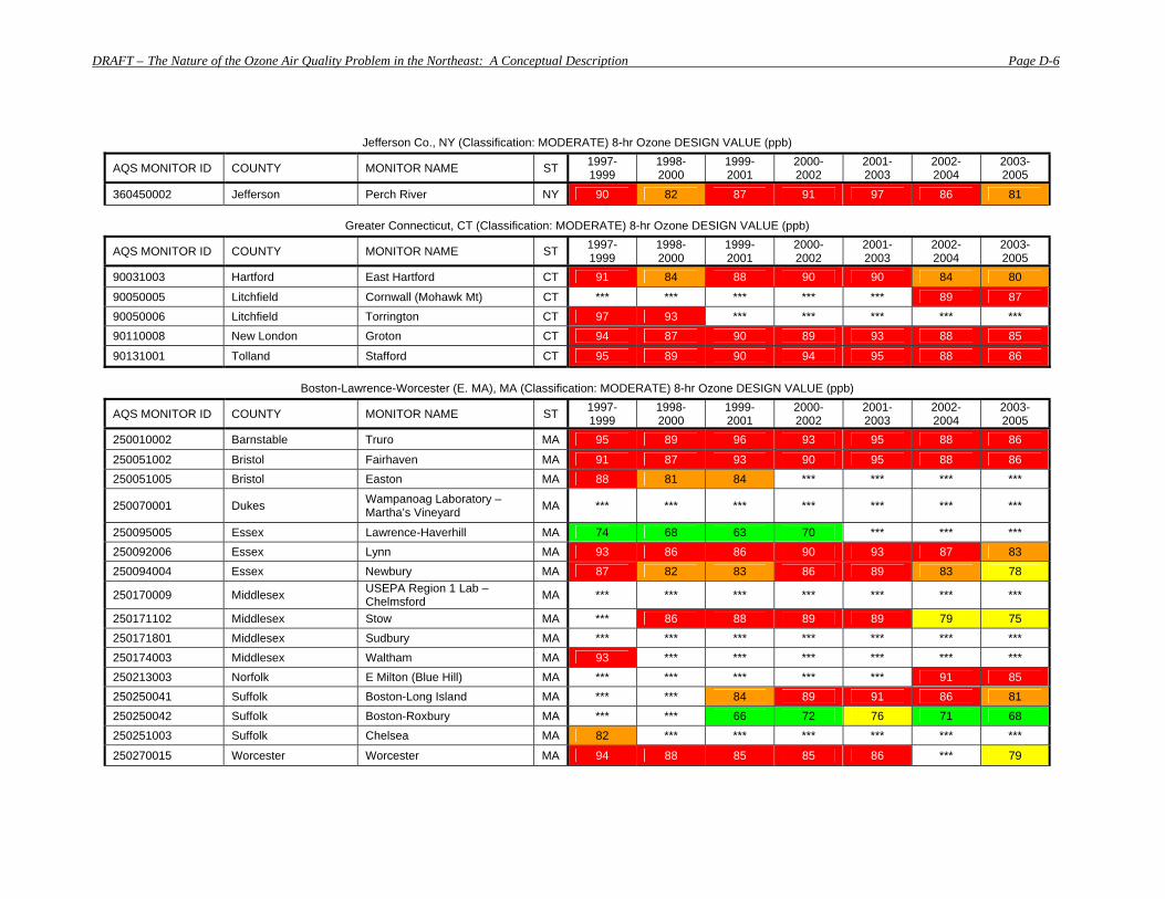
DRAFT – The Nature of the Ozone Air Quality Problem in the Northeast: A Conceptual Description Page D-6
Jefferson Co., NY (Classification: MODERATE) 8-hr Ozone DESIGN VALUE (ppb)
AQS MONITOR ID COUNTY MONITOR NAME ST 1997-1999
1998-2000
1999-2001
2000-2002
2001-2003
2002-2004
2003-2005
360450002 Jefferson Perch River NY 90 82 87 91 97 86 81
Greater Connecticut, CT (Classification: MODERATE) 8-hr Ozone DESIGN VALUE (ppb)
AQS MONITOR ID COUNTY MONITOR NAME ST 1997-1999
1998-2000
1999-2001
2000-2002
2001-2003
2002-2004
2003-2005
90031003 Hartford East Hartford CT 91 84 88 90 90 84 80
90050005 Litchfield Cornwall (Mohawk Mt) CT *** *** *** *** *** 89 87 90050006 Litchfield Torrington CT 97 93 *** *** *** *** *** 90110008 New London Groton CT 94 87 90 89 93 88 85
90131001 Tolland Stafford CT 95 89 90 94 95 88 86
Boston-Lawrence-Worcester (E. MA), MA (Classification: MODERATE) 8-hr Ozone DESIGN VALUE (ppb)
AQS MONITOR ID COUNTY MONITOR NAME ST 1997-1999
1998-2000
1999-2001
2000-2002
2001-2003
2002-2004
2003-2005
250010002 Barnstable Truro MA 95 89 96 93 95 88 86
250051002 Bristol Fairhaven MA 91 87 93 90 95 88 86 250051005 Bristol Easton MA 88 81 84 *** *** *** ***
250070001 Dukes Wampanoag Laboratory – Martha’s Vineyard MA *** *** *** *** *** *** ***
250095005 Essex Lawrence-Haverhill MA 74 68 63 70 *** *** *** 250092006 Essex Lynn MA 93 86 86 90 93 87 83 250094004 Essex Newbury MA 87 82 83 86 89 83 78
250170009 Middlesex USEPA Region 1 Lab – Chelmsford MA *** *** *** *** *** *** ***
250171102 Middlesex Stow MA *** 86 88 89 89 79 75 250171801 Middlesex Sudbury MA *** *** *** *** *** *** *** 250174003 Middlesex Waltham MA 93 *** *** *** *** *** *** 250213003 Norfolk E Milton (Blue Hill) MA *** *** *** *** *** 91 85 250250041 Suffolk Boston-Long Island MA *** *** 84 89 91 86 81 250250042 Suffolk Boston-Roxbury MA *** *** 66 72 76 71 68 250251003 Suffolk Chelsea MA 82 *** *** *** *** *** ***
250270015 Worcester Worcester MA 94 88 85 85 86 *** 79
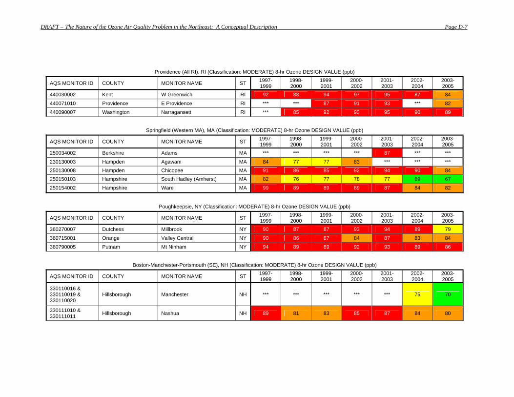
DRAFT – The Nature of the Ozone Air Quality Problem in the Northeast: A Conceptual Description Page D-7
Providence (All RI), RI (Classification: MODERATE) 8-hr Ozone DESIGN VALUE (ppb)
AQS MONITOR ID COUNTY MONITOR NAME ST 1997-1999
1998-2000
1999-2001
2000-2002
2001-2003
2002-2004
2003-2005
440030002 Kent W Greenwich RI 92 88 94 97 95 87 84
440071010 Providence E Providence RI *** *** 87 91 93 *** 82
440090007 Washington Narragansett RI *** 85 92 93 95 90 89
Springfield (Western MA), MA (Classification: MODERATE) 8-hr Ozone DESIGN VALUE (ppb)
AQS MONITOR ID COUNTY MONITOR NAME ST 1997-1999
1998-2000
1999-2001
2000-2002
2001-2003
2002-2004
2003-2005
250034002 Berkshire Adams MA *** *** *** *** 87 *** ***
230130003 Hampden Agawam MA 84 77 77 83 *** *** *** 250130008 Hampden Chicopee MA 91 86 85 92 94 90 84 250150103 Hampshire South Hadley (Amherst) MA 82 76 77 78 77 69 67
250154002 Hampshire Ware MA 99 89 89 89 87 84 82
Poughkeepsie, NY (Classification: MODERATE) 8-hr Ozone DESIGN VALUE (ppb)
AQS MONITOR ID COUNTY MONITOR NAME ST 1997-1999
1998-2000
1999-2001
2000-2002
2001-2003
2002-2004
2003-2005
360270007 Dutchess Millbrook NY 90 87 87 93 94 89 79
360715001 Orange Valley Central NY 90 86 87 84 87 83 84
360790005 Putnam Mt Ninham NY 94 89 89 92 93 89 86
Boston-Manchester-Portsmouth (SE), NH (Classification: MODERATE) 8-hr Ozone DESIGN VALUE (ppb)
AQS MONITOR ID COUNTY MONITOR NAME ST 1997-1999
1998-2000
1999-2001
2000-2002
2001-2003
2002-2004
2003-2005
330110016 & 330110019 & 330110020
Hillsborough Manchester NH *** *** *** *** *** 75 70
330111010 & 330111011 Hillsborough Nashua NH 89 81 83 85 87 84 80
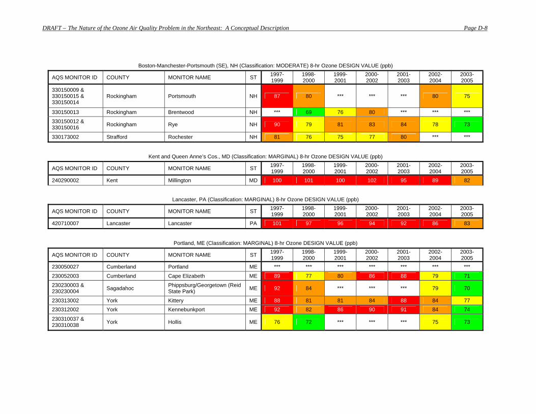
DRAFT – The Nature of the Ozone Air Quality Problem in the Northeast: A Conceptual Description Page D-8
Boston-Manchester-Portsmouth (SE), NH (Classification: MODERATE) 8-hr Ozone DESIGN VALUE (ppb)
AQS MONITOR ID COUNTY MONITOR NAME ST 1997-1999
1998-2000
1999-2001
2000-2002
2001-2003
2002-2004
2003-2005
330150009 & 330150015 & 330150014
Rockingham Portsmouth NH 87 80 *** *** *** 80 75
330150013 Rockingham Brentwood NH *** 69 76 80 *** *** ***
330150012 & 330150016 Rockingham Rye NH 90 79 81 83 84 78 73
330173002 Strafford Rochester NH 81 76 75 77 80 *** ***
Kent and Queen Anne’s Cos., MD (Classification: MARGINAL) 8-hr Ozone DESIGN VALUE (ppb)
AQS MONITOR ID COUNTY MONITOR NAME ST 1997-1999
1998-2000
1999-2001
2000-2002
2001-2003
2002-2004
2003-2005
240290002 Kent Millington MD 100 101 100 102 95 89 82
Lancaster, PA (Classification: MARGINAL) 8-hr Ozone DESIGN VALUE (ppb)
AQS MONITOR ID COUNTY MONITOR NAME ST 1997-1999
1998-2000
1999-2001
2000-2002
2001-2003
2002-2004
2003-2005
420710007 Lancaster Lancaster PA 101 97 96 94 92 86 83
Portland, ME (Classification: MARGINAL) 8-hr Ozone DESIGN VALUE (ppb)
AQS MONITOR ID COUNTY MONITOR NAME ST 1997-1999
1998-2000
1999-2001
2000-2002
2001-2003
2002-2004
2003-2005
230050027 Cumberland Portland ME *** *** *** *** *** *** ***
230052003 Cumberland Cape Elizabeth ME 89 77 80 86 88 79 71
230230003 & 230230004 Sagadahoc Phippsburg/Georgetown (Reid
State Park) ME 92 84 *** *** *** 79 70
230313002 York Kittery ME 88 81 81 84 88 84 77 230312002 York Kennebunkport ME 92 82 86 90 91 84 74
230310037 & 230310038 York Hollis ME 76 72 *** *** *** 75 73

DRAFT – The Nature of the Ozone Air Quality Problem in the Northeast: A Conceptual Description Page D-9
Buffalo-Niagara Falls, NY (Classification: SUBPART 1) 8-hr Ozone DESIGN VALUE (ppb)
AQS MONITOR ID COUNTY MONITOR NAME ST 1997-1999
1998-2000
1999-2001
2000-2002
2001-2003
2002-2004
2003-2005
360290002 Erie Amherst NY 85 89 92 97 99 91 86
360631006 Niagara Middleport NY 86 85 87 91 95 89 86
Youngstown-Warren-Sharon, OH-PA (Classification: SUBPART 1) 8-hr Ozone DESIGN VALUE (ppb)
AQS MONITOR ID COUNTY MONITOR NAME ST 1997-1999
1998-2000
1999-2001
2000-2002
2001-2003
2002-2004
2003-2005
390990009 & 390990013 Mahoning Youngstown - Oakhill OH 91 89 86 87 89 85 80
391550008 & 391550011 Trumbull Warren-Trumbull County OH 95 91 88 90 95 91 86
391550009 Trumbull Kinsman OH 95 91 87 87 90 87 83
420850100 Mercer Farrell PA 96 92 88 92 94 88 83
Pittsburgh-Beaver Valley, PA (Classification: SUBPART 1) 8-hr Ozone DESIGN VALUE (ppb)
AQS MONITOR ID COUNTY MONITOR NAME ST 1997-1999
1998-2000
1999-2001
2000-2002
2001-2003
2002-2004
2003-2005
420030008 Allegheny Lawrenceville PA 91 88 85 89 92 87 81
420030010 Allegheny Pittsburg PA *** 91 92 93 93 86 84 420030067 Allegheny South Fayette PA 99 96 90 90 91 87 82 420030088 Allegheny Penn Hills PA 92 91 88 *** *** *** *** 420031005 Allegheny Harrison Township PA 101 94 92 95 92 87 81 420050001 Armstrong Kittanning PA 86 93 92 91 93 88 84 420070002 Beaver Hookstown PA 92 89 88 90 94 90 84 420070005 Beaver Brighton Township PA 91 90 89 90 92 87 81 420070014 Beaver Beaver Falls PA 90 89 85 88 86 81 75 421250005 Washington Charleroi PA 101 94 87 86 89 84 80 421250200 Washington Washington PA 91 88 86 86 88 82 81 421255001 Washington Florence PA 91 90 88 88 87 82 78 421290006 Westmoreland Murrysville PA 85 81 80 81 84 81 80
421290008 Westmoreland Greensburg PA *** *** 86 86 91 87 82
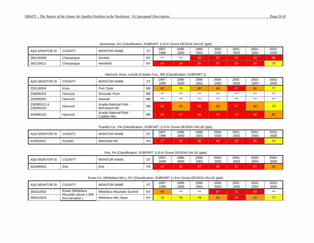
DRAFT – The Nature of the Ozone Air Quality Problem in the Northeast: A Conceptual Description Page D-10
Jamestown, NY (Classification: SUBPART 1) 8-hr Ozone DESIGN VALUE (ppb)
AQS MONITOR ID COUNTY MONITOR NAME ST 1997-1999
1998-2000
1999-2001
2000-2002
2001-2003
2002-2004
2003-2005
360130006 Chautauqua Dunkirk NY *** *** 89 92 94 93 89
360130011 Chautauqua Westfield NY 89 88 85 87 89 85 79
Hancock, Knox, Lincoln & Waldo Cos., ME (Classification: SUBPART 1)
AQS MONITOR ID COUNTY MONITOR NAME ST 1997-1999
1998-2000
1999-2001
2000-2002
2001-2003
2002-2004
2003-2005
230130004 Knox Port Clyde ME 82 76 80 83 87 81 77
230090401 Hancock Schoodic Point ME *** *** *** *** *** *** *** 230090001 Hancock Seawall ME *** *** *** *** *** *** ***
230090101 & 230090103 Hancock Acadia National Park -
McFarland Hill ME 85 83 85 84 87 80 75
230090102 Hancock Acadia National Park - Cadillac Mtn. ME 89 87 89 93 94 88 82
Franklin Co., PA (Classification: SUBPART 1) 8-hr Ozone DESIGN VALUE (ppb)
AQS MONITOR ID COUNTY MONITOR NAME ST 1997-1999
1998-2000
1999-2001
2000-2002
2001-2003
2002-2004
2003-2005
420550001 Franklin Methodist Hill PA 97 95 92 94 93 85 75
Erie, PA (Classification: SUBPART 1) 8-hr Ozone DESIGN VALUE (ppb)
AQS MONITOR ID COUNTY MONITOR NAME ST 1997-1999
1998-2000
1999-2001
2000-2002
2001-2003
2002-2004
2003-2005
420490003 Erie Erie PA 93 90 87 88 92 87 83
Essex Co. (Whiteface Mtn.), NY (Classification: SUBPART 1) 8-hr Ozone DESIGN VALUE (ppb)
AQS MONITOR ID COUNTY MONITOR NAME ST 1997-1999
1998-2000
1999-2001
2000-2002
2001-2003
2002-2004
2003-2005
360310002 Whiteface Mountain Summit NY 80 *** *** 87 91 89 ***
360310003
Essex (Whiteface Mountain above 1,900 foot elevation ) Whiteface Mtn. Base NY 79 76 78 82 88 83 77
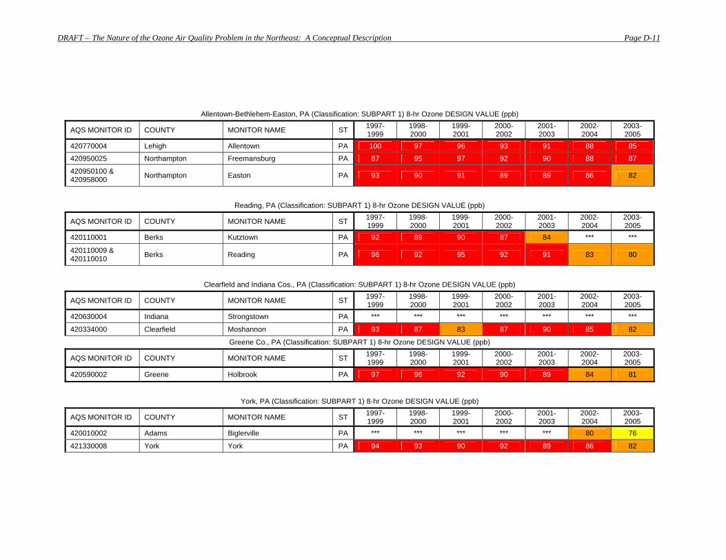
DRAFT – The Nature of the Ozone Air Quality Problem in the Northeast: A Conceptual Description Page D-11
Allentown-Bethlehem-Easton, PA (Classification: SUBPART 1) 8-hr Ozone DESIGN VALUE (ppb)
AQS MONITOR ID COUNTY MONITOR NAME ST 1997-1999
1998-2000
1999-2001
2000-2002
2001-2003
2002-2004
2003-2005
420770004 Lehigh Allentown PA 100 97 96 93 91 88 85
420950025 Northampton Freemansburg PA 87 95 97 92 90 88 87
420950100 & 420958000 Northampton Easton PA 93 90 91 89 89 86 82
Reading, PA (Classification: SUBPART 1) 8-hr Ozone DESIGN VALUE (ppb)
AQS MONITOR ID COUNTY MONITOR NAME ST 1997-1999
1998-2000
1999-2001
2000-2002
2001-2003
2002-2004
2003-2005
420110001 Berks Kutztown PA 92 89 90 87 84 *** ***
420110009 & 420110010 Berks Reading PA 96 92 95 92 91 83 80
Clearfield and Indiana Cos., PA (Classification: SUBPART 1) 8-hr Ozone DESIGN VALUE (ppb)
AQS MONITOR ID COUNTY MONITOR NAME ST 1997-1999
1998-2000
1999-2001
2000-2002
2001-2003
2002-2004
2003-2005
420630004 Indiana Strongstown PA *** *** *** *** *** *** ***
420334000 Clearfield Moshannon PA 93 87 83 87 90 85 82
Greene Co., PA (Classification: SUBPART 1) 8-hr Ozone DESIGN VALUE (ppb)
AQS MONITOR ID COUNTY MONITOR NAME ST 1997-1999
1998-2000
1999-2001
2000-2002
2001-2003
2002-2004
2003-2005
420590002 Greene Holbrook PA 97 96 92 90 89 84 81
York, PA (Classification: SUBPART 1) 8-hr Ozone DESIGN VALUE (ppb)
AQS MONITOR ID COUNTY MONITOR NAME ST 1997-1999
1998-2000
1999-2001
2000-2002
2001-2003
2002-2004
2003-2005
420010002 Adams Biglerville PA *** *** *** *** *** 80 76
421330008 York York PA 94 93 90 92 89 86 82
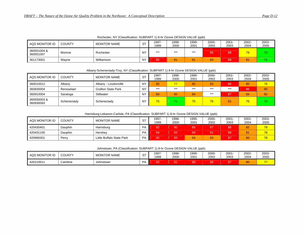
DRAFT – The Nature of the Ozone Air Quality Problem in the Northeast: A Conceptual Description Page D-12
Rochester, NY (Classification: SUBPART 1) 8-hr Ozone DESIGN VALUE (ppb)
AQS MONITOR ID COUNTY MONITOR NAME ST 1997-1999
1998-2000
1999-2001
2000-2002
2001-2003
2002-2004
2003-2005
360551004 & 360551007 Monroe Rochester NY *** *** *** 85 88 79 73
361173001 Wayne Williamson NY 86 81 81 83 88 81 71
Albany-Schenectady-Troy, NY (Classification: SUBPART 1) 8-hr Ozone DESIGN VALUE (ppb)
AQS MONITOR ID COUNTY MONITOR NAME ST 1997-1999
1998-2000
1999-2001
2000-2002
2001-2003
2002-2004
2003-2005
360010012 Albany Albany - Loudonville NY 80 77 80 83 86 80 76
360830004 Rensselaer Grafton State Park NY *** *** *** *** *** 86 80 360910004 Saratoga Stillwater NY 84 80 84 *** 87 84 82
360930003 & 360930093 Schenectady Schenectady NY 75 71 75 76 81 76 74
Harrisburg-Lebanon-Carlisle, PA (Classification: SUBPART 1) 8-hr Ozone DESIGN VALUE (ppb)
AQS MONITOR ID COUNTY MONITOR NAME ST 1997-1999
1998-2000
1999-2001
2000-2002
2001-2003
2002-2004
2003-2005
420430401 Dauphin Harrisburg PA 92 90 86 87 86 82 78
420431100 Dauphin Hershey PA 94 93 94 91 88 81 78
420990301 Perry Little Buffalo State Park PA 90 85 84 83 87 80 78
Johnstown, PA (Classification: SUBPART 1) 8-hr Ozone DESIGN VALUE (ppb)
AQS MONITOR ID COUNTY MONITOR NAME ST 1997-1999
1998-2000
1999-2001
2000-2002
2001-2003
2002-2004
2003-2005
420210011 Cambria Johnstown PA 93 91 88 88 87 80 77
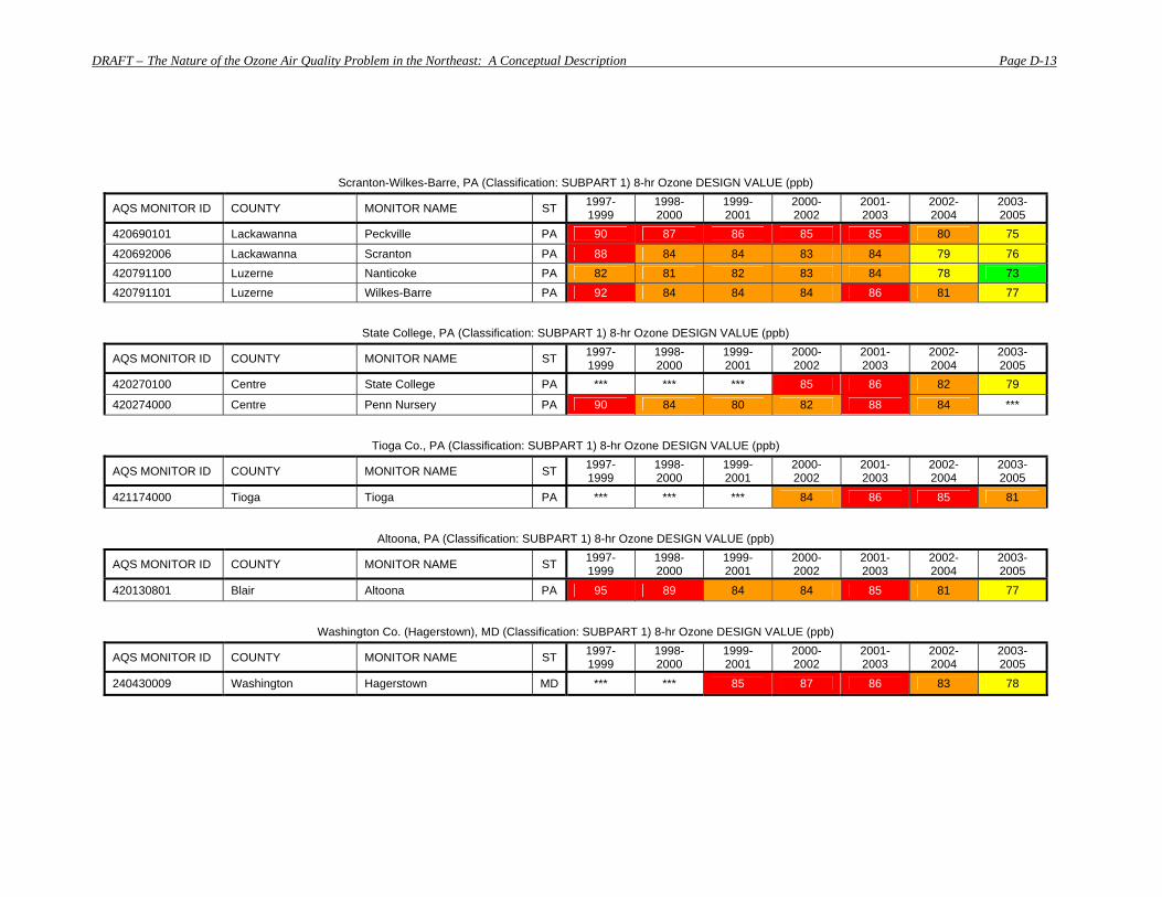
DRAFT – The Nature of the Ozone Air Quality Problem in the Northeast: A Conceptual Description Page D-13
Scranton-Wilkes-Barre, PA (Classification: SUBPART 1) 8-hr Ozone DESIGN VALUE (ppb)
AQS MONITOR ID COUNTY MONITOR NAME ST 1997-1999
1998-2000
1999-2001
2000-2002
2001-2003
2002-2004
2003-2005
420690101 Lackawanna Peckville PA 90 87 86 85 85 80 75
420692006 Lackawanna Scranton PA 88 84 84 83 84 79 76 420791100 Luzerne Nanticoke PA 82 81 82 83 84 78 73 420791101 Luzerne Wilkes-Barre PA 92 84 84 84 86 81 77
State College, PA (Classification: SUBPART 1) 8-hr Ozone DESIGN VALUE (ppb)
AQS MONITOR ID COUNTY MONITOR NAME ST 1997-1999
1998-2000
1999-2001
2000-2002
2001-2003
2002-2004
2003-2005
420270100 Centre State College PA *** *** *** 85 86 82 79
420274000 Centre Penn Nursery PA 90 84 80 82 88 84 ***
Tioga Co., PA (Classification: SUBPART 1) 8-hr Ozone DESIGN VALUE (ppb)
AQS MONITOR ID COUNTY MONITOR NAME ST 1997-1999
1998-2000
1999-2001
2000-2002
2001-2003
2002-2004
2003-2005
421174000 Tioga Tioga PA *** *** *** 84 86 85 81
Altoona, PA (Classification: SUBPART 1) 8-hr Ozone DESIGN VALUE (ppb)
AQS MONITOR ID COUNTY MONITOR NAME ST 1997-1999
1998-2000
1999-2001
2000-2002
2001-2003
2002-2004
2003-2005
420130801 Blair Altoona PA 95 89 84 84 85 81 77
Washington Co. (Hagerstown), MD (Classification: SUBPART 1) 8-hr Ozone DESIGN VALUE (ppb)
AQS MONITOR ID COUNTY MONITOR NAME ST 1997-1999
1998-2000
1999-2001
2000-2002
2001-2003
2002-2004
2003-2005
240430009 Washington Hagerstown MD *** *** 85 87 86 83 78
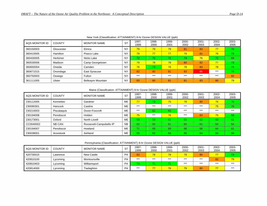
DRAFT – The Nature of the Ozone Air Quality Problem in the Northeast: A Conceptual Description Page D-14
New York (Classification: ATTAINMENT) 8-hr Ozone DESIGN VALUE (ppb)
AQS MONITOR ID COUNTY MONITOR NAME ST 1997-1999
1998-2000
1999-2001
2000-2002
2001-2003
2002-2004
2003-2005
360150003 Gloucester Elmira NY 79 79 79 81 83 77 70
360410005 Hamilton Piseco Lake NY 79 77 77 79 81 76 73 360430005 Herkimer Nicks Lake NY 72 70 72 74 76 72 69 360530006 Madison Camp Georgetown NY 79 78 78 80 82 77 73 360650004 Oneida Camden NY 76 73 76 78 83 78 72 360671015 Onondaga East Syracuse NY 82 80 81 83 85 *** 74 360750003 Oswego Fulton NY *** *** *** *** *** *** 82
361111005 Ulster Belleayre Mountain NY 83 80 81 81 83 80 79
Maine (Classification: ATTAINMENT) 8-hr Ozone DESIGN VALUE (ppb)
AQS MONITOR ID COUNTY MONITOR NAME ST 1997-1999
1998-2000
1999-2001
2000-2002
2001-2003
2002-2004
2003-2005
230112005 Kennebec Gardiner ME 77 73 75 78 80 76 70
230090301 Hancock Castine ME *** *** *** *** *** 75 70 230210003 Piscataquis Dover-Foxcroft ME *** 62 65 *** *** *** *** 230194008 Penobscot Holden ME 75 *** 76 *** 83 75 68 230173001 Oxford North Lovell ME 59 58 61 60 62 60 61 CC0040002 NB CAN Roosevelt-Campobello IP NB 62 60 61 60 61 54 54 230194007 Penobscot Howland ME 71 68 69 68 68 64 61
230038001 Aroostook Ashland ME 65 62 64 65 64 63 60
Pennsylvania (Classification: ATTAINMENT) 8-hr Ozone DESIGN VALUE (ppb)
AQS MONITOR ID COUNTY MONITOR NAME ST 1997-1999
1998-2000
1999-2001
2000-2002
2001-2003
2002-2004
2003-2005
420730015 Lawrence New Castle PA 83 78 78 78 80 77 73
420810100 Lycoming Montoursville PA *** *** *** *** *** 82 79 420810403 Lycoming Williamsport PA 74 71 71 *** *** *** ***
420814000 Lycoming Tiadaghton PA *** 77 76 79 80 77 ***
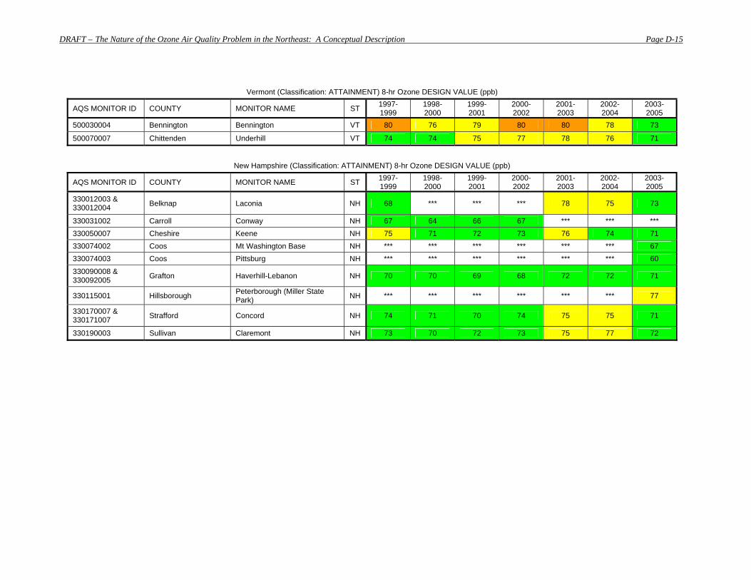
DRAFT – The Nature of the Ozone Air Quality Problem in the Northeast: A Conceptual Description Page D-15
Vermont (Classification: ATTAINMENT) 8-hr Ozone DESIGN VALUE (ppb)
AQS MONITOR ID COUNTY MONITOR NAME ST 1997-1999
1998-2000
1999-2001
2000-2002
2001-2003
2002-2004
2003-2005
500030004 Bennington Bennington VT 80 76 79 80 80 78 73
500070007 Chittenden Underhill VT 74 74 75 77 78 76 71
New Hampshire (Classification: ATTAINMENT) 8-hr Ozone DESIGN VALUE (ppb)
AQS MONITOR ID COUNTY MONITOR NAME ST 1997-1999
1998-2000
1999-2001
2000-2002
2001-2003
2002-2004
2003-2005
330012003 & 330012004 Belknap Laconia NH 68 *** *** *** 78 75 73
330031002 Carroll Conway NH 67 64 66 67 *** *** *** 330050007 Cheshire Keene NH 75 71 72 73 76 74 71 330074002 Coos Mt Washington Base NH *** *** *** *** *** *** 67 330074003 Coos Pittsburg NH *** *** *** *** *** *** 60
330090008 & 330092005 Grafton Haverhill-Lebanon NH 70 70 69 68 72 72 71
330115001 Hillsborough Peterborough (Miller State Park) NH *** *** *** *** *** *** 77
330170007 & 330171007 Strafford Concord NH 74 71 70 74 75 75 71
330190003 Sullivan Claremont NH 73 70 72 73 75 77 72
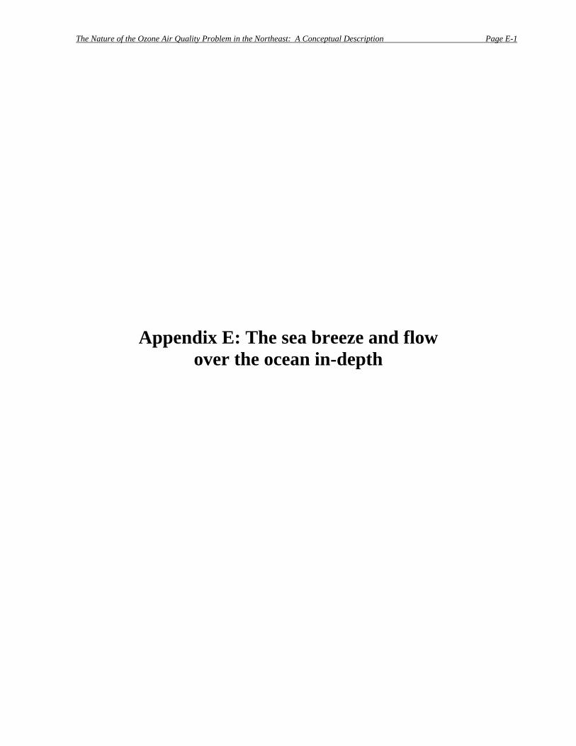
The Nature of the Ozone Air Quality Problem in the Northeast: A Conceptual Description Page E-1
Appendix E: The sea breeze and flow over the ocean in-depth
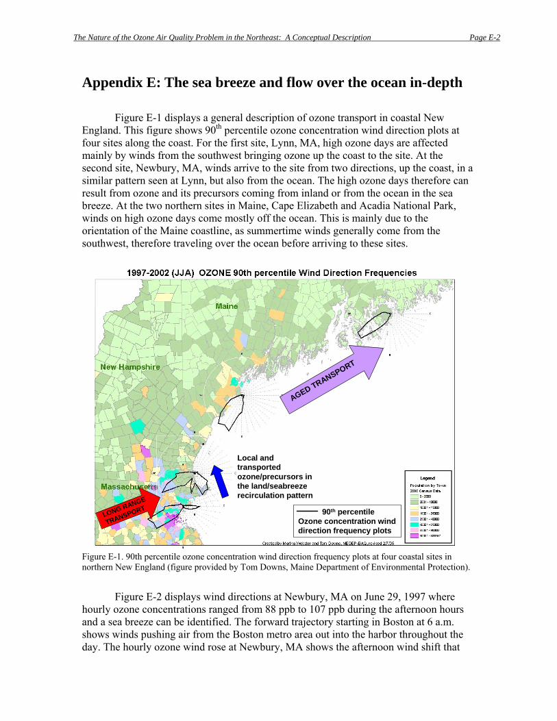
The Nature of the Ozone Air Quality Problem in the Northeast: A Conceptual Description Page E-2
Appendix E: The sea breeze and flow over the ocean in-depth
Figure E-1 displays a general description of ozone transport in coastal New England. This figure shows 90th percentile ozone concentration wind direction plots at four sites along the coast. For the first site, Lynn, MA, high ozone days are affected mainly by winds from the southwest bringing ozone up the coast to the site. At the second site, Newbury, MA, winds arrive to the site from two directions, up the coast, in a similar pattern seen at Lynn, but also from the ocean. The high ozone days therefore can result from ozone and its precursors coming from inland or from the ocean in the sea breeze. At the two northern sites in Maine, Cape Elizabeth and Acadia National Park, winds on high ozone days come mostly off the ocean. This is mainly due to the orientation of the Maine coastline, as summertime winds generally come from the southwest, therefore traveling over the ocean before arriving to these sites.
AGED TRANSPORT
LONG RANGE
TRANSPORT 90th percentile Ozone concentration wind direction frequency plots
Local and transported ozone/precursors in the land/seabreezerecirculation pattern
AGED TRANSPORT
LONG RANGE
TRANSPORT 90th percentile Ozone concentration wind direction frequency plots
Local and transported ozone/precursors in the land/seabreezerecirculation pattern
AGED TRANSPORT
LONG RANGE
TRANSPORT 90th percentile Ozone concentration wind direction frequency plots
Local and transported ozone/precursors in the land/seabreezerecirculation pattern
Figure E-1. 90th percentile ozone concentration wind direction frequency plots at four coastal sites in northern New England (figure provided by Tom Downs, Maine Department of Environmental Protection).
Figure E-2 displays wind directions at Newbury, MA on June 29, 1997 where
hourly ozone concentrations ranged from 88 ppb to 107 ppb during the afternoon hours and a sea breeze can be identified. The forward trajectory starting in Boston at 6 a.m. shows winds pushing air from the Boston metro area out into the harbor throughout the day. The hourly ozone wind rose at Newbury, MA shows the afternoon wind shift that
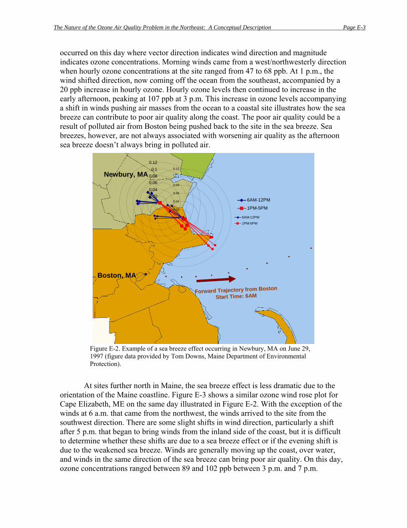
The Nature of the Ozone Air Quality Problem in the Northeast: A Conceptual Description Page E-3
occurred on this day where vector direction indicates wind direction and magnitude indicates ozone concentrations. Morning winds came from a west/northwesterly direction when hourly ozone concentrations at the site ranged from 47 to 68 ppb. At 1 p.m., the wind shifted direction, now coming off the ocean from the southeast, accompanied by a 20 ppb increase in hourly ozone. Hourly ozone levels then continued to increase in the early afternoon, peaking at 107 ppb at 3 p.m. This increase in ozone levels accompanying a shift in winds pushing air masses from the ocean to a coastal site illustrates how the sea breeze can contribute to poor air quality along the coast. The poor air quality could be a result of polluted air from Boston being pushed back to the site in the sea breeze. Sea breezes, however, are not always associated with worsening air quality as the afternoon sea breeze doesn’t always bring in polluted air.
00.020.040.060.080.1
0.121
2 3 4 56 7 8 9
1 01 11 21 3
1 4 1 51 6 1 7
1 81 9
2 02 12 2
2 32 4
2 52 6
2 72 8
2 9
3 03 1
3 23 3
3 43 5
3 6
3 73 8
3 94 0
4 14 2
4 3
4 44 5
4 6
4 7
4 84 9
5 0
5 1
5 2
5 3
5 4
5 5
5 6
5 7
5 8
5 9
6 0
6 1
6 2
6 3
6 4
6 5
6 6
6 7
6 8
6 9
7 0
7 1
7 2
7 3
7 4
7 5
7 6
7 7
7 8
7 9
8 0
8 1
8 2
8 3
8 4
8 5
8 6
8 7
8 8
8 9
9 0
9 1
9 2
9 3
9 4
9 5
9 6
9 7
9 8
9 9
1 0 0
1 0 1
1 0 2
1 0 3
1 0 4
1 0 5
1 0 6
1 0 7
1 0 8
1 0 9
1 1 0
1 1 1
1 1 2
1 1 3
1 1 4
1 1 5
1 1 6
1 1 7
1 1 8
1 1 9
1 2 0
1 2 1
1 2 2
1 2 3
1 2 4
1 2 5
1 2 6
1 2 7
1 2 8
1 2 9
1 3 0
1 3 1
1 3 2
1 3 31 3 4
1 3 5
1 3 6
1 3 71 3 8
1 3 9
1 4 01 4 1
1 4 21 4 3
1 4 41 4 5
1 4 61 4 7
1 4 8
1 4 91 5 0
1 5 11 5 2
1 5 31 5 4
1 5 51 5 6
1 5 71 5 8
1 5 91 6 0
1 6 11 6 21 6 3
1 6 41 6 51 6 6
1 6 71 6 81 6 91 7 0
1 7 11 7 21 7 31 7 41 7 51 7 6
1 7 71 7 81 7 91 8 0
1 8 1
1 8 21 8 31 8 41 8 51 8 61 8 71 8 81 8 9
1 9 01 9 11 9 21 9 3
1 9 41 9 51 9 61 9 7
1 9 81 9 9
2 0 02 0 12 0 2
2 0 32 0 4
2 0 52 0 6
2 0 72 0 8
2 0 9
2 1 02 1 1
2 1 22 1 3
2 1 42 1 5
2 1 6
2 1 72 1 8
2 1 92 2 0
2 2 12 2 2
2 2 3
2 2 42 2 5
2 2 6
2 2 7
2 2 82 2 9
2 3 0
2 3 1
2 3 2
2 3 3
2 3 4
2 3 5
2 3 6
2 3 7
2 3 8
2 3 9
2 4 0
2 4 1
2 4 2
2 4 3
2 4 4
2 4 5
2 4 6
2 4 7
2 4 8
2 4 9
2 5 0
2 5 1
2 5 2
2 5 3
2 5 4
2 5 5
2 5 6
2 5 7
2 5 8
2 5 9
2 6 0
2 6 1
2 6 2
2 6 3
2 6 4
2 6 5
2 6 6
2 6 7
2 6 8
2 6 9
2 7 0
2 7 1
2 7 2
2 7 3
2 7 4
2 7 5
2 7 6
2 7 7
2 7 8
2 7 9
2 8 0
2 8 1
2 8 2
2 8 3
2 8 4
2 8 5
2 8 6
2 8 7
2 8 8
2 8 9
2 9 0
2 9 1
2 9 2
2 9 3
2 9 4
2 9 5
2 9 6
2 9 7
2 9 8
2 9 9
3 0 0
3 0 1
3 0 2
3 0 3
3 0 4
3 0 5
3 0 6
3 0 7
3 0 8
3 0 9
3 1 0
3 1 1
3 1 2
3 1 33 1 4
3 1 5
3 1 6
3 1 73 1 8
3 1 9
3 2 03 2 1
3 2 23 2 3
3 2 43 2 5
3 2 63 2 7
3 2 8
3 2 93 3 0
3 3 13 3 2
3 3 33 3 4
3 3 53 3 6
3 3 73 3 8
3 3 93 4 0
3 4 13 4 23 4 3
3 4 43 4 53 4 6
3 4 73 4 83 4 93 5 0
3 5 13 5 23 5 33 5 43 5 53 5 6
3 5 73 5 83 5 93 6 0
6AM-12PM
1PM-5PM
Forward Trajectory from BostonStart Time: 6AM
Boston, MA
Newbury, MA
0
0.02
0.04
0.06
0.08
0.1
0.12
6AM-12PM
1PM-5PM
Figure E-2. Example of a sea breeze effect occurring in Newbury, MA on June 29, 1997 (figure data provided by Tom Downs, Maine Department of Environmental Protection).
At sites further north in Maine, the sea breeze effect is less dramatic due to the
orientation of the Maine coastline. Figure E-3 shows a similar ozone wind rose plot for Cape Elizabeth, ME on the same day illustrated in Figure E-2. With the exception of the winds at 6 a.m. that came from the northwest, the winds arrived to the site from the southwest direction. There are some slight shifts in wind direction, particularly a shift after 5 p.m. that began to bring winds from the inland side of the coast, but it is difficult to determine whether these shifts are due to a sea breeze effect or if the evening shift is due to the weakened sea breeze. Winds are generally moving up the coast, over water, and winds in the same direction of the sea breeze can bring poor air quality. On this day, ozone concentrations ranged between 89 and 102 ppb between 3 p.m. and 7 p.m.
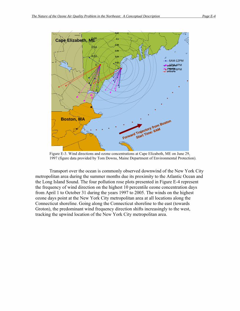
The Nature of the Ozone Air Quality Problem in the Northeast: A Conceptual Description Page E-4
0
0.02
0.04
0.06
0.08
0.1
0.12
6AM-12PM1PM-4PM5PM-6PM
Forward Trajectory from Boston
Start Time: 6AM
Cape Elizabeth, ME
Boston, MA
0
0.02
0.04
0.06
6AM-12PM1PM-4PM5PM-6PM0
0.02
0.04
0.06
0.08
0.1
0.12
6AM-12PM1PM-4PM5PM-6PM
Forward Trajectory from Boston
Start Time: 6AM
Cape Elizabeth, ME
Boston, MA
0
0.02
0.04
0.06
0.08
0.1
0.12
6AM-12PM1PM-4PM5PM-6PM
Forward Trajectory from Boston
Start Time: 6AM
0
0.02
0.04
0.06
0.08
0.1
0.12
6AM-12PM1PM-4PM5PM-6PM
Forward Trajectory from Boston
Start Time: 6AM
0
0.02
0.04
0.06
0.08
0.1
0.12
6AM-12PM1PM-4PM5PM-6PM
Forward Trajectory from Boston
Start Time: 6AM
Cape Elizabeth, ME
Boston, MA
0
0.02
0.04
0.06
6AM-12PM1PM-4PM5PM-6PM
Figure E-3. Wind directions and ozone concentrations at Cape Elizabeth, ME on June 29, 1997 (figure data provided by Tom Downs, Maine Department of Environmental Protection).
Transport over the ocean is commonly observed downwind of the New York City
metropolitan area during the summer months due its proximity to the Atlantic Ocean and the Long Island Sound. The four pollution rose plots presented in Figure E-4 represent the frequency of wind direction on the highest 10 percentile ozone concentration days from April 1 to October 31 during the years 1997 to 2005. The winds on the highest ozone days point at the New York City metropolitan area at all locations along the Connecticut shoreline. Going along the Connecticut shoreline to the east (towards Groton), the predominant wind frequency direction shifts increasingly to the west, tracking the upwind location of the New York City metropolitan area.

The Nature of the Ozone Air Quality Problem in the Northeast: A Conceptual Description Page E-5
Figure E-4. Wind rose plots along Connecticut shoreline for the time period April 1 to October 31 during the years 1997 through 2005. The elongated red outlines pointing to the southwest to west are wind directions on the highest 10 percentile ozone concentration days at four Connecticut coastal locations. For comparison, the blue outlines are the wind rose plots for all days over the same period. The high ozone day wind rose plots indicate pollution flow over Long Island Sound that tracks the upwind location of the New York City metropolitan area (figure from Tom Downs, Maine Department of the Environment).
Each plot shows frequency of high ozone increases as the wind points up LIS towards emission-rich areas of the Northeast corridor.
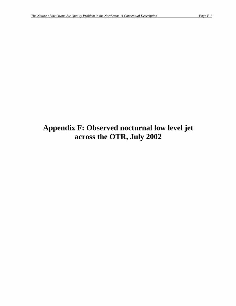
The Nature of the Ozone Air Quality Problem in the Northeast: A Conceptual Description Page F-1
Appendix F: Observed nocturnal low level jet across the OTR, July 2002

The Nature of the Ozone Air Quality Problem in the Northeast: A Conceptual Description Page F-2
Appendix F: Observed nocturnal low level jet across the OTR, July 2002
An example of the nocturnal low level jet across the OTR can be seen on the nights of July 22 through July 24, 2002, as night time winds at altitudes between 450 m and 1500 m were observed at several coastal sites. Figure F-1 shows wind profiler data on the night of July 22-July 23, 2002 for five sites along the east coast: Fort Meade, MD (FME), Orange, MA (ORE), Stow, MA (STW), Appledore Island, ME (ADI), and Pease Air Force Base, NH (PSE). These wind “barb” plots show wind direction (direction of arrow indicating where wind is coming from), wind speed (wind barb color), time of day (UTC time, x-axis), and altitude (meters, y-axis). The location of the nocturnal low level jet appears within the circle in each wind barb plot of Figure F-1. The figure shows a weak nocturnal low level jet at the southernmost site, Fort Meade, with wind speeds of 15 to 25 knots between 300 m and 500 m in the early part of the night. Further north, the nocturnal low level jet is more pronounced with wind speeds between 500 m and 1500 m above ground reaching 40 knots. Figure F-1 shows on this day the nocturnal low level jet extending from Maryland up through southern Maine. In addition, the wind barb plots show the northeasterly direction of the nocturnal low level jet. Above this jet, we see slower winds coming from the west to all the sites.
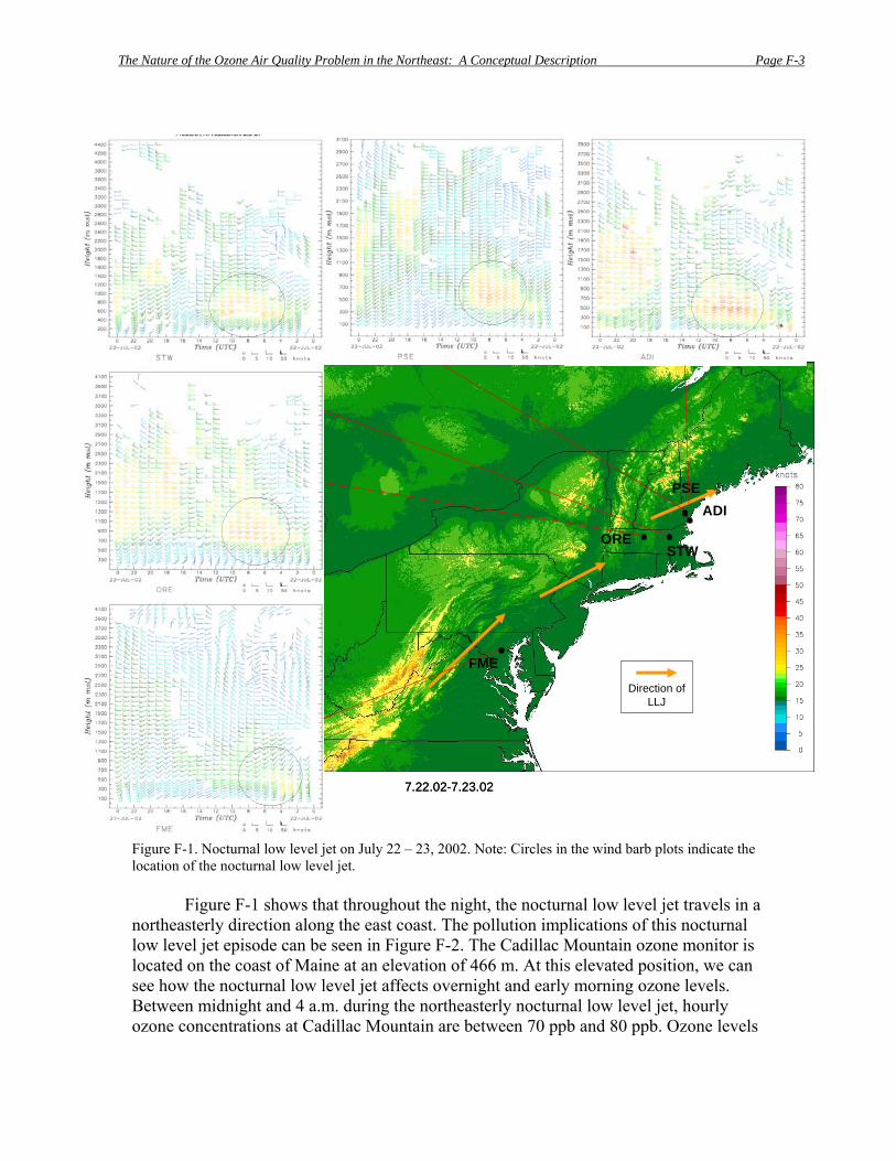
The Nature of the Ozone Air Quality Problem in the Northeast: A Conceptual Description Page F-3
7.22.02-7.23.02
FME
ORESTW
ADIPSE
Direction ofLLJ
7.22.02-7.23.02
FME
ORESTW
ADIPSE
Direction ofLLJ
Figure F-1. Nocturnal low level jet on July 22 – 23, 2002. Note: Circles in the wind barb plots indicate the location of the nocturnal low level jet.
Figure F-1 shows that throughout the night, the nocturnal low level jet travels in a northeasterly direction along the east coast. The pollution implications of this nocturnal low level jet episode can be seen in Figure F-2. The Cadillac Mountain ozone monitor is located on the coast of Maine at an elevation of 466 m. At this elevated position, we can see how the nocturnal low level jet affects overnight and early morning ozone levels. Between midnight and 4 a.m. during the northeasterly nocturnal low level jet, hourly ozone concentrations at Cadillac Mountain are between 70 ppb and 80 ppb. Ozone levels
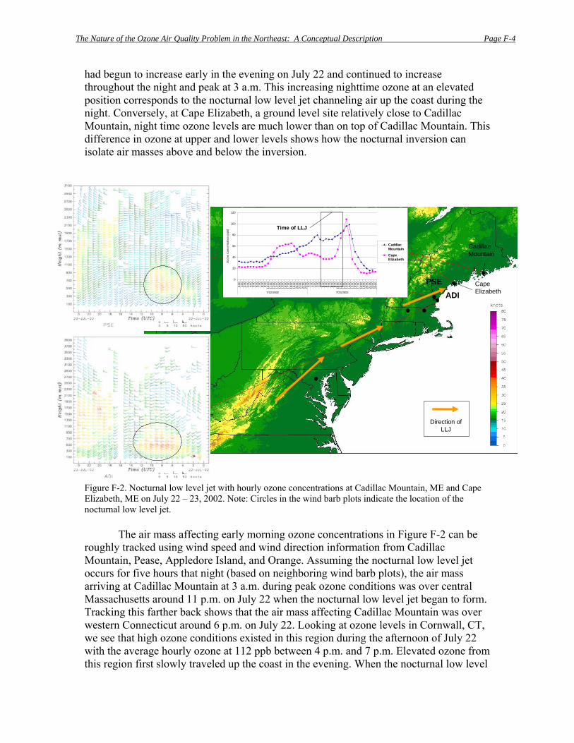
The Nature of the Ozone Air Quality Problem in the Northeast: A Conceptual Description Page F-4
had begun to increase early in the evening on July 22 and continued to increase throughout the night and peak at 3 a.m. This increasing nighttime ozone at an elevated position corresponds to the nocturnal low level jet channeling air up the coast during the night. Conversely, at Cape Elizabeth, a ground level site relatively close to Cadillac Mountain, night time ozone levels are much lower than on top of Cadillac Mountain. This difference in ozone at upper and lower levels shows how the nocturnal inversion can isolate air masses above and below the inversion.
ADIPSE
Direction ofLLJ
CadillacMountain
CapeElizabeth
0
20
40
60
80
100
120
0:00
1:00
2:00
3:00
4:00
5:00
6:00
7:00
8:00
9:00
10:0
011
:00
12:0
013
:00
14:0
015
:00
16:0
017
:00
18:0
019
:00
20:0
021
:00
22:0
023
:00
0:00
1:00
2:00
3:00
4:00
5:00
6:00
7:00
8:00
9:00
10:0
011
:00
12:0
013
:00
14:0
015
:00
16:0
017
:00
18:0
019
:00
20:0
021
:00
22:0
023
:00
7/22/2002 7/23/2002
Ozo
ne C
once
ntra
tion
(ppb
)
CadillacMountain
CapeElizabeth
Time of LLJ
Figure F-2. Nocturnal low level jet with hourly ozone concentrations at Cadillac Mountain, ME and Cape Elizabeth, ME on July 22 – 23, 2002. Note: Circles in the wind barb plots indicate the location of the nocturnal low level jet.
The air mass affecting early morning ozone concentrations in Figure F-2 can be roughly tracked using wind speed and wind direction information from Cadillac Mountain, Pease, Appledore Island, and Orange. Assuming the nocturnal low level jet occurs for five hours that night (based on neighboring wind barb plots), the air mass arriving at Cadillac Mountain at 3 a.m. during peak ozone conditions was over central Massachusetts around 11 p.m. on July 22 when the nocturnal low level jet began to form. Tracking this farther back shows that the air mass affecting Cadillac Mountain was over western Connecticut around 6 p.m. on July 22. Looking at ozone levels in Cornwall, CT, we see that high ozone conditions existed in this region during the afternoon of July 22 with the average hourly ozone at 112 ppb between 4 p.m. and 7 p.m. Elevated ozone from this region first slowly traveled up the coast in the evening. When the nocturnal low level

The Nature of the Ozone Air Quality Problem in the Northeast: A Conceptual Description Page F-5
jet formed, it quickly pushed ozone up the coast affecting ozone levels at Cadillac Mountain, an elevated site in the jet, in the early morning hours (~3 a.m.).
Figure F-3 shows wind profiler information for the next day, July 24, 2002. In this case we see a stronger nocturnal low level jet between midnight and 8am that originates further to the south. The Fort Meade and Rutgers (RUT) sites show the nocturnal low level jet in the early part of the evening with flow in the northeasterly direction. At higher altitudes slower winds from the west pass over the nocturnal low level jet. Further north, a strong nocturnal low level jet can be seen at Stow, Appledore Island, and Pease. It is difficult to determine if a nocturnal low level jet exists at Orange as high winds continue at the upper altitudes and data are missing for the highest altitudes. Figure F-3 demonstrates an example of the nocturnal low level jet passing along the east coast as far south as Maryland and as far north as southern Maine.
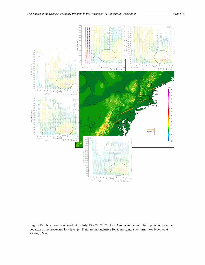
The Nature of the Ozone Air Quality Problem in the Northeast: A Conceptual Description Page F-6
Figure F-3. Nocturnal low level jet on July 23 – 24, 2002. Note: Circles in the wind barb plots indicate the location of the nocturnal low level jet. Data are inconclusive for identifying a nocturnal low level jet at Orange, MA.
FME
ORE STW
ADI
PSE
RUT
Direction ofLLJ
FME
ORE STW
ADI
PSE
RUT
Direction ofLLJ
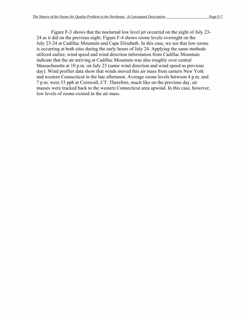
The Nature of the Ozone Air Quality Problem in the Northeast: A Conceptual Description Page F-7
Figure F-3 shows that the nocturnal low level jet occurred on the night of July 23-24 as it did on the previous night. Figure F-4 shows ozone levels overnight on the July 23-24 at Cadillac Mountain and Cape Elizabeth. In this case, we see that low ozone is occurring at both sites during the early hours of July 24. Applying the same methods utilized earlier, wind speed and wind direction information from Cadillac Mountain indicate that the air arriving at Cadillac Mountain was also roughly over central Massachusetts at 10 p.m. on July 23 (same wind direction and wind speed as previous day). Wind profiler data show that winds moved this air mass from eastern New York and western Connecticut in the late afternoon. Average ozone levels between 4 p.m. and 7 p.m. were 53 ppb at Cornwall, CT. Therefore, much like on the previous day, air masses were tracked back to the western Connecticut area upwind. In this case, however, low levels of ozone existed in the air mass.
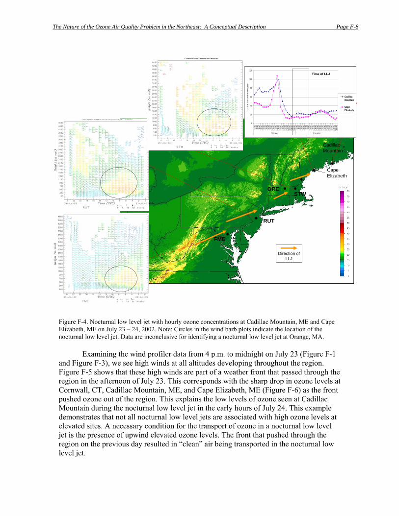
The Nature of the Ozone Air Quality Problem in the Northeast: A Conceptual Description Page F-8
Figure F-4. Nocturnal low level jet with hourly ozone concentrations at Cadillac Mountain, ME and Cape Elizabeth, ME on July 23 – 24, 2002. Note: Circles in the wind barb plots indicate the location of the nocturnal low level jet. Data are inconclusive for identifying a nocturnal low level jet at Orange, MA.
Examining the wind profiler data from 4 p.m. to midnight on July 23 (Figure F-1 and Figure F-3), we see high winds at all altitudes developing throughout the region. Figure F-5 shows that these high winds are part of a weather front that passed through the region in the afternoon of July 23. This corresponds with the sharp drop in ozone levels at Cornwall, CT, Cadillac Mountain, ME, and Cape Elizabeth, ME (Figure F-6) as the front pushed ozone out of the region. This explains the low levels of ozone seen at Cadillac Mountain during the nocturnal low level jet in the early hours of July 24. This example demonstrates that not all nocturnal low level jets are associated with high ozone levels at elevated sites. A necessary condition for the transport of ozone in a nocturnal low level jet is the presence of upwind elevated ozone levels. The front that pushed through the region on the previous day resulted in “clean” air being transported in the nocturnal low level jet.
FME
ORESTW
RUT
Direction ofLLJ
CadillacMountain
CapeElizabeth
0
20
40
60
80
100
120
0:0
01:0
02:0
03:0
04:0
05:0
06:0
07:0
08:0
09:0
010:0
011:0
012:0
013:0
014:0
015:0
016:0
017:0
018:0
019:0
020:0
021:0
022:0
023:0
00:0
01:0
02:0
03:0
04:0
05:0
06:0
07:0
08:0
09:0
010:0
011:0
012:0
013:0
014:0
015:0
016:0
017:0
018:0
019:0
020:0
021:0
022:0
023:0
0
7/23/2002 7/24/2002
Ozone C
oncentr
ation (
ppb)
CadillacMountain
CapeElizabeth
Time of LLJ
0
20
40
60
80
100
120
0:0
01:0
02:0
03:0
04:0
05:0
06:0
07:0
08:0
09:0
010:0
011:0
012:0
013:0
014:0
015:0
016:0
017:0
018:0
019:0
020:0
021:0
022:0
023:0
00:0
01:0
02:0
03:0
04:0
05:0
06:0
07:0
08:0
09:0
010:0
011:0
012:0
013:0
014:0
015:0
016:0
017:0
018:0
019:0
020:0
021:0
022:0
023:0
0
7/23/2002 7/24/2002
Ozone C
oncentr
ation (
ppb)
CadillacMountain
CapeElizabeth
Time of LLJ

The Nature of the Ozone Air Quality Problem in the Northeast: A Conceptual Description Page F-9
8AM 7.23.02 8PM 7.23.028AM 7.23.028AM 7.23.02 8PM 7.23.028PM 7.23.02
Figure F-5. Weather map displaying a front passing through the East on July 23, 2002.
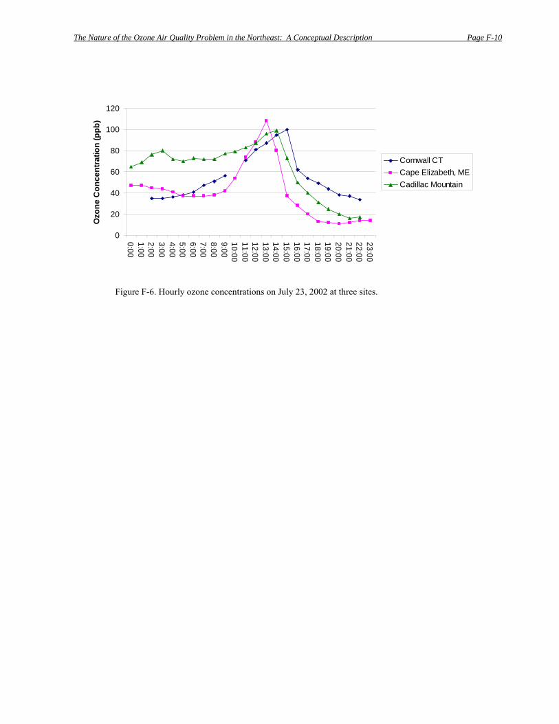
The Nature of the Ozone Air Quality Problem in the Northeast: A Conceptual Description Page F-10
0
20
40
60
80
100
120
0:001:002:003:004:005:006:007:008:009:0010:0011:0012:0013:0014:0015:0016:0017:0018:0019:0020:0021:0022:0023:00
Ozo
ne C
once
ntra
tion
(ppb
)
Cornwall CTCape Elizabeth, MECadillac Mountain
Figure F-6. Hourly ozone concentrations on July 23, 2002 at three sites.
The Nature of the Ozone Air Quality Problem in the Northeast: A Conceptual Description Page G-1
Appendix G: Contributions to the ozone reservoir
The Nature of the Ozone Air Quality Problem in the Northeast: A Conceptual Description Page G-1
Appendix G: Contributions to the ozone reservoir Contributions to the ozone reservoir can come from two sources. The first is from
the residual local ozone and precursors in the atmosphere at sunset. The second is from transport of ozone and precursors from outside of the local region. To identify these outside sources, Taubman et al. (2006) have made an analysis of the complete set of aircraft flights undertaken by RAMMPP between 1992 and 2003. Initially, the data were divided into morning and afternoon profiles to identify diurnal patterns. Little diurnal variation was observed in the carbon monoxide and sulfur dioxide profiles. The ozone values were greater in the afternoon than the morning, while ozone in the lower free troposphere (i.e., above the boundary level), where long range transport is possible, was consistently ~55 ppb. Transport patterns and source regions during summertime haze and ozone episodes were analyzed with a cluster analysis of back trajectory data. Eight clusters were identified, which were then divided into morning and afternoon profiles. Table G-1 lists the characteristics of each cluster, and Figure G-1 shows the back trajectories calculated for each profile divided by cluster at an altitude of 2000 meters. The median profile values were calculated and statistical differences were determined using a nonparametric procedure. When the greatest trajectory density lay over the northern Ohio River Valley, which has large NOX and sulfur dioxide sources, the results were large ozone values, a large SO2/CO ratio, large scattering particles, and high aerosol optical depth over the mid-Atlantic U.S. In contrast, relatively clean conditions over the mid-Atlantic occurred when the greatest trajectory density lay over the southern Ohio River Valley and nearly missed many large NOX and SO2 sources. The greatest afternoon ozone values occurred during periods of stagnation that were most conducive to photochemical production. The least pollution occurred when flow from the north-northwest was too fast for pollution to accumulate and when flow was from the north, where there are few urban or industrial sources.
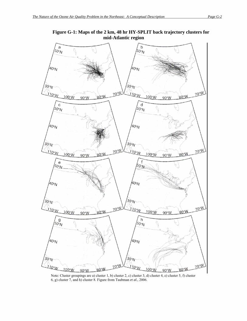
The Nature of the Ozone Air Quality Problem in the Northeast: A Conceptual Description Page G-2
Figure G-1: Maps of the 2 km, 48 hr HY-SPLIT back trajectory clusters for mid-Atlantic region
Note: Cluster groupings are a) cluster 1, b) cluster 2, c) cluster 3, d) cluster 4, e) cluster 5, f) cluster 6, g) cluster 7, and h) cluster 8. Figure from Taubman et al., 2006.

The Nature of the Ozone Air Quality Problem in the Northeast: A Conceptual Description Page G-3
Ozone transport over several hundred kilometers into the mid-Atlantic U.S. was estimated by calculating the ratio of the residual layer ozone between 500 m and 2 km in the upwind morning profiles to the downwind afternoon boundary layer values between 100 m and 2 km. The greatest level of transported ozone (69-82 percent) occurred when the maximum trajectory density lay over the southern and northern Ohio River Valley (clusters 1, 2, 4, and 6); ~59 percent of the total profiles). The least amount of transported ozone (55-58 percent) was associated with fast southwesterly flow (cluster 8; ~3 percent of the total profiles), fast north-northwesterly flow or clean northerly flow from regions with relatively few urban or industrial pollution sources (clusters 5 and 7; ~6 percent of the total profiles), and stagnant conditions within the mid-Atlantic conducive to greater local ozone production (cluster 3; ~27 percent of the total profiles). The average amount of ozone transported into the Baltimore-Washington urban corridor is 64 percent of the total observed ozone in the afternoon boundary layer. If the background ozone is removed, then this value is lowered to 55 percent.
When trajectory density plots were overlaid on maps with the largest annual NOX and SO2 emitters, specific source regions were identified. The results indicate that the areas of maximum trajectory density together with wind speed are effective predictors of regional pollution and loadings. Additionally, due to the Lagrangian nature of the dataset, the regionally transported contribution to the total afternoon boundary layer column ozone content in each cluster could be quantified.
Table G-1. Cluster groups for air mass trajectories into mid-Atlantic Region
Cluster Description Upwind Region
1 Large ozone values, large SO2/CO ratio, large highly scattering particles. Moderate northwesterly flow – aged point source air.
Northern Ohio River Valley
2 Small ozone values, large SO2/CO ratio. Northwesterly flow at higher wind speeds than Cluster 1 – aged point source air.
Northern Ohio River Valley, extending into the Great Lakes region
3 Large ozone values, small SO2/CO ratio. Stagnant conditions with light southerly flow.
Central mid-Atlantic region
4 Small ozone values, small SO2/CO ratio. Moderate southwesterly flow, small pollution loading – fewer point sources.
Southern Ohio River Valley
5 Fairly fast north-northwesterly flow. Flow too fast for pollution to accumulate from source region.
Northern Great Lakes
6 Moderately large ozone values, SO2/CO ratio very large, smaller less scattering particles. Northwesterly flow, but faster wind speeds than Clusters 1 and 2. Crosses several large SO2 and NOX sources.
Northern Ohio River Valley
7 Least pollution of any of the clusters. Flow is out of the north. Relatively cool, dry continental air.
Eastern Ontario, western Quebec
8 Small ozone values, small SO2/CO ratio. Fast southwest flow. Very few trajectories.
Vicinity of Texas

The Nature of the Ozone Air Quality Problem in the Northeast: A Conceptual Description Page G-4
Reference Taubman, B.F., J.C. Hains, A.M. Thompson, L.T. Marufu, B.G. Doddridge, J.W. Stehr, C.A. Peity, and R.R. Dickerson. “Aircraft vertical profiles of trace gas and aerosol pollution over the mid-Atlantic United States: Statistics and meteorological cluster analysis.” J. Geophys. Res. 111, D10S07, doi:10.1029/2005JD006196, 2006.