Appendix A Additional Data Details

51

Appendix A Additional Data Details

Appendix A.1 List of Cities Used in Estimation Table A.1 City List

Akron, OH Albany, NY Allentown, PA Altoona, PA Amsterdam, NY Atlanta, GA Atlantic City, NJ Auburn, NY Augusta, GA Baltimore, MD Bay City, MI Bayonne, NJ Berkeley, CA Binghamton, NY Birmingham, AL Boston, MA Bridgeport, CT Brockton, MA Buffalo, NY Butte, MT Cambridge, MA Camden, NJ Canton, OH Cedar Rapids, IA Charleston, SC Charlotte, NC Chattanooga, TN Chelsea, MA Chester, PA Chicago, IL Cincinnati, OH Cleveland, OH Columbus, OH Covington, KY Dallas, TX Davenport, IA

Dayton, OH Decatur, IL Denver, CO Des Moines, IA Detroit, MI Dubuque, IA Duluth, MN East Orange, NJ East St. Louis, IL El Paso, TX Elizabeth, NJ Elmira, NY Erie, PA Evansville, IN Everett, MA Fall River, MA Fitchburg, MA Flint, MI Fort Wayne, IN Forth Worth, TX Galveston, TX Grand Rapids, MI Hamilton, OH Harrisburg, PA Hartford, CT Haverhill, MA Hoboken, NJ Holyoke, MA Houston, TX Huntington, WV Indianapolis, IN Jackson, MI Jacksonville, FL Jamestown, NY Jersey City, NJ Johnstown, PA

Joliet, IL Kalamazoo, MI Kansas City, KS Kansas City, MO Knoxville, TN La Crosse, WI Lancaster, PA Lansing, MI Lawrence, MA Lexington, KY Lima, OH Lincoln, NE Little Rock, AR Los Angeles, CA Louisville, KY Lowell, MA Lynn, MA Macon, GA Malden, MA Manchester, NH McKeesport, PA Memphis, TN Milwaukee, WI Minneapolis, MN Mobile, AL Montgomery, AL Mount Vernon, NY Nashville, TN New Bedford, MA New Britain, CT New Castle, PA New Haven, CT New Orleans, LA New York, NY Newark, NJ Newton, MA

Niagara Falls, NY Norfolk, VA Oakland, CA Oklahoma City, OK Omaha, NE Oshkosh, WI Pasadena, CA Passaic, NJ Paterson, NJ Pawtucket, RI Peoria, IL Perth Amboy, NJ Philadelphia, PA Pittsburgh, PA Pittsfield, MA Portland, ME Portland, OR Portsmouth, VA Providence, RI Pueblo, CO Quincy, IL Quincy, MA Racine, WI Reading, PA Richmond, VA Roanoke, VA Rochester, NY Rockford, IL Sacramento, CA Saginaw, MI Saint Joseph, MO Saint Louis, MO Saint Paul, MN Salem, MA San Antonio, TX San Diego, CA

San Francisco, CA Savannah, GA Schenectady, NY Scranton, PA Seattle, WA Sioux City, IA Somerville, MA South Bend, IN Spokane, WA Springfield, IL Springfield, MA Springfield, MO Springfield, OH Superior, WI Syracuse, NY Tacoma, WA Tampa, FL Taunton, MA Terre Haute, IN Toledo, OH Topeka, KS Trenton, NJ Troy, NY Utica, NY Washington, DC Waterbury, CT Wheeling, WV Wichita, KS Wilkes-Barre, PA Williamsport, PA Wilmington, DE Woonsocket, RI Worcester, MA Yonkers, NY York, PA Youngstown, OH

52

Appendix A.2 List of One Digit Occupations Table A.2 Occupations List

1 Digit Occupation 3 Digit 1950 Codes Avg Occ Score Examples Farmer/Farm Laborer 100-123,810-840 11.2 Farm owners, Farm laborers Laborer/Other 910-970 19.2 Laborers, Fishermen, Gardeners Services 700-790 21.0 Barbers, Janitors, Policemen Clerical 300-390 24.5 Bank tellers, Telephone operators Operatives 600-690 25.4 Blasters, Oilers, Welders Sales 400-490 25.6 Advertising agents, Sales clerks Craftsmen 500-595 30.8 Blacksmiths, Electricians Managers/Officials 200-290 41.8 Managers, Public Officials Professional/Technical 000-099 46.9 Accountants, Scientists, Doctors

Appendix A.3 Additional Detail on Tabellini (2020) Instrument

Our baseline analysis uses the following instrument for predicted immigration changes in each city (equation (3) in the text):

∆𝑃𝑃𝐹𝐹𝑃𝑃𝑃𝑃𝐹𝐹𝐹𝐹𝐹𝐹𝐹𝐹𝐹𝐹𝐹𝐹𝐹𝐹𝐹𝐹𝑔𝑔𝑐𝑐𝑐𝑐 =1𝑃𝑃�𝑐𝑐,𝑐𝑐

�𝜔𝜔𝑖𝑖,𝑐𝑐,1900𝐹𝐹𝐹𝐹𝐹𝐹𝐹𝐹𝑔𝑔𝑖𝑖,−𝑐𝑐,𝑐𝑐𝑖𝑖

where ∆𝑃𝑃𝐹𝐹𝑃𝑃𝑃𝑃𝐹𝐹𝐹𝐹𝐹𝐹𝐹𝐹𝐹𝐹𝐹𝐹𝐹𝐹𝐹𝐹𝑔𝑔𝑐𝑐𝑐𝑐 is the predicted share of the population who are immigrants for each city 𝐹𝐹 in each time period 𝑡𝑡 ∈ {1920,1930}, 𝑃𝑃�𝑐𝑐,𝑐𝑐 is the predicted population of city 𝐹𝐹 in the time period 𝑡𝑡, 𝜔𝜔𝑖𝑖,𝑐𝑐,1900 is the fraction of all immigrants of region of origin 𝐹𝐹 who reside in city 𝐹𝐹 in the year 1900, and 𝐹𝐹𝐹𝐹𝐹𝐹𝐹𝐹𝑔𝑔𝑖𝑖,−𝑐𝑐,𝑐𝑐 is the total immigrants in-flows to the United States from region 𝐹𝐹 between time periods 𝑡𝑡 − 10 and 𝑡𝑡, omitting the inflows that ultimately resided in city 𝐹𝐹. We take this instrument directly from Tabellini (2020), who uses 16 European regions of origin in constructing immigrant flows and immigrant enclaves: UK, Ireland, Denmark, Finland, Norway, Sweden, Germany, Poland, Russia, Eastern Europe (Yugoslavia, Czechoslovakia, etc.), Austria-Hungary, Switzerland, France, Belgium-Netherlands, Greece-Portugal-Spain, and Italy. Both the fraction of each immigrant origin region living in each city and total immigrant inflows from each region are totaled using full count Census data. The predicted population, 𝑃𝑃�𝑐𝑐,𝑐𝑐, for each city is constructed as the population of each city in the year 1900 multiplied by the average urban population growth between the two Census years being studied. Formally, this is constructed as:

𝑃𝑃�𝑐𝑐,𝑐𝑐 = 𝑃𝑃𝑃𝑃𝑃𝑃𝑐𝑐,1900 ∗ 𝑔𝑔𝑐𝑐−𝑐𝑐 where 𝑔𝑔𝑐𝑐−𝑐𝑐 is the average urban population growth between Census years 𝑡𝑡 and 𝑡𝑡 − 10, constructed leaving out the population growth in city 𝐹𝐹. Appendix B Robustness Exercises

In this Appendix, we provide a variety of robustness exercises for our primary findings. In examining the robustness of our results, we primarily focus on our average findings at the individual level, reported in Table 5 in the paper. Differences in findings at the individual level

53

for workers of different ages, skill, or migration status are comparable to those reported in the paper unless indicated otherwise. Appendix B.1 Relationship between Linking and Changes in Immigration

A potential threat to identification in specifications using linked data to study individual outcomes is the possibility that the probability of being able to link workers across Census years is correlated with the treatment of predicted changes in immigration. Relatedly, we might also be concerned that the probability of linking the FamilySearch data to the Ancestry/IPUMS labor market data or the probability of reporting a “not yet classified” occupation is correlated with treatment. We provide some evidence that this is not the case in Table B.1. Here we estimate a two-stage least squares specification (in levels) considering the relationship between our treatment of the predicted fraction of immigrants at the city level and outcomes of the probability of linking individual data, either across time (Column 1) or between FamilySearch and Ancestry for either the first or second Census wave we observe workers (Columns 2 and 3), and the probability of observing a not yet classified occupation.

Our estimates find no statistically significant relationship between our treatment and the probability of linking over time or being observed in a not yet classified. We do, however, find a statistically significant relationship between being able to match FamilySearch to Ancestry/IPUMS labor market data in cities with increased immigration in the first year we observe workers. We emphasize, however, that the baseline match rate here is extremely high at 98%, and the increased probability of linking means that cities experiencing large changes in immigration may have had match rates closer to 99%. Given these high match rates and the comparatively small overall effect of this linking to labor data, we do not consider this further. Appendix B.2 Robustness to Reweighting Individual Specifications

One difference between our local labor market estimates and our individual level estimates is how we weight observations, as our local labor market estimates place equal weight on each city, but our individual estimates place equal weight on each individual. In Table B.2 we replicate the our baseline individual findings (originally reported in Table 5) where we reweight each observation to be one divided by the total native city population, mimicking the weighting approach in our local labor market results.

Using this weighting scheme reduces the precision of our estimates considerably and also reduces the magnitude of our coefficients. However, we find the same qualitative patterns as in our baseline findings – increases in immigration increased out-migration, increased labor force participation, had no measurable impact on income, and provided some insurance against downward occupational switches. These results are suggestive that the effects of increased immigration may be different between larger and smaller cities, as larger cities will receive greater weight when we weight on the basis of people. However, we still find that relative to our local labor market specifications, the impacts of immigration for individual workers are substantially smaller. Appendix B.3 Robustness to Including Sacramento and New Bedford

54

In our baseline results, we exclude the cities of New Bedford, MA and Sacramento, CA, following Tabellini (2020), who reports that some data is unavailable for these cities in the year 1920. We do not face this limitation, and so in Table B.3 we report individual outcomes with these two cities. We find very similar results to our baseline specifications, the notable exception that the inclusion of these two cities greatly attenuates the effect of immigration on changes in labor force participation. While unreported, we also find that the labor force participation results are greatly attenuated at the local labor market level when including these cities. Examining heterogeneous treatment effects by age, also unreported, we observe that the pattern of increased labor force participation by the young and reduced by the old has is the same, but the relative magnitudes of the increases for the young and the decreases have changed in such a way as to reduce the average. Appendix B.4 Robustness to Using Variation from Immigration Policy and World War I

As an alternative identification strategy, we also consider (as in Ager and Hansen (2017), Tabellini (2020) and Abramitzky et al. (2019)) constructing predicted immigration for each city on not only the pre-existing settlement patterns of immigrants of different regions of origin, but also on the basis of changes in U.S. immigration policy in the early 20th century. Immigration from non-allied European countries was substantially reduced during World War I and then the Immigration Acts of the 1920s placed quotas on immigration from certain regions of the world. Thus, these changes in policy provide an alternative way of constructing plausibly exogenous variation in immigration over time. Formally, we construct two instruments, one for WWI (affecting immigration between 1910 and 1920) and one for the Immigration Acts of the 1920s (affecting immigration between 1920 and 1930), as follows. Predicted immigration between 1910 and 1920 is constructed as:

∆𝑃𝑃𝐹𝐹𝑃𝑃𝑃𝑃𝐹𝐹𝐹𝐹𝐹𝐹𝐹𝐹𝐹𝐹𝐹𝐹𝐹𝐹𝐹𝐹𝑔𝑔𝑐𝑐,1920 =1

𝑃𝑃�𝑐𝑐,1920�𝜔𝜔𝑖𝑖,𝑐𝑐,1900𝐹𝐹𝐹𝐹𝐹𝐹𝐹𝐹𝑔𝑔𝑖𝑖,1910𝑖𝑖

(1[𝐴𝐴𝐴𝐴𝐴𝐴𝐹𝐹𝑃𝑃𝑠𝑠𝑖𝑖] − 1)

where 1[𝐴𝐴𝐴𝐴𝐴𝐴𝐹𝐹𝑃𝑃𝑠𝑠𝑖𝑖] is an indicator for whether or not region 𝐹𝐹 was part of the Allied side in World War I and 𝐹𝐹𝐹𝐹𝐹𝐹𝐹𝐹𝑔𝑔𝑖𝑖,1910 is the total inflows of immigrants to the US between 1900 and 1910 from region 𝐹𝐹. Intuitively, for Allied regions, the instrument would predict no change in immigration over this time period, whereas the non-allied regions, the instrument predicts a substantial decline in immigration. For the period 1920 to 1930, the instrument is constructed as

∆𝑃𝑃𝐹𝐹𝑃𝑃𝑃𝑃𝐹𝐹𝐹𝐹𝐹𝐹𝐹𝐹𝐹𝐹𝐹𝐹𝐹𝐹𝐹𝐹𝑔𝑔𝑐𝑐,1930 =1

𝑃𝑃�𝑐𝑐,1930�𝜔𝜔𝑖𝑖,𝑐𝑐,1900�𝑄𝑄𝑄𝑄𝑃𝑃𝑡𝑡𝐹𝐹𝑖𝑖 − 𝐹𝐹𝐹𝐹𝐹𝐹𝐹𝐹𝑔𝑔𝑖𝑖,1920�𝑖𝑖

where 𝑄𝑄𝑄𝑄𝑃𝑃𝑡𝑡𝐹𝐹𝑖𝑖 is the sum of the yearly quota for region 𝐹𝐹 imposed by the Immigration Acts of 1921 and 1924 and 𝐹𝐹𝐹𝐹𝐹𝐹𝐹𝐹𝑔𝑔𝑖𝑖,1920 is the total inflows of immigrants to the US between 1910 and 1920 from region 𝐹𝐹. Intuitively, for regions facing low quotas, which heavily restricted immigration from those regions, the instrument predicts substantially lower inflows. We report the first stage of these additional instruments in Appendix C and report our findings at the individual level using these instruments in Table B.4. Our results using these alternate instruments are very similar to our baseline results. While unreported, we also find that our results are very similar if we just use the WWI instrument.

55

Appendix B.5 Robustness to Including Not Yet Classified Occupation Observations Our baseline results omit workers whose occupation is coded as “Not Yet Classified,” as we do not have data on their occupational income scores. Alternatively, we could include these workers, as they do not have missing data for migration or labor force status, and we impute their income scores using the state average income score each year.1 We report the baseline individual results with these observations included in Table B.5. These results are almost identical to our original results for migration and labor force status, and very similar for occupation switching and occupational income scores. The one notable difference here is that when including these not yet classified occupations with imputations for income scores, there is now a statistically significant reduction in the likelihood of making an upward occupational switch. However, given that this result is sensitive to the imputation of income scores for certain workers, we do not focus on it further. Appendix B.6 Robustness Checks from Tabellini (2020) Following Tabellini (2020), we also present our results allowing for differential trends in certain city characteristics. Given that our local labor market strategy draws explicitly from Tabellini (2020), we focus on presenting our individual results with these differential trends, as this is what is novel to our paper. Table B.6 presents our results for migration, labor force participation and occupational income scores allowing for differential trends in city characteristics. The set of city characteristics we focus on is a measure of predicted industrialization (from Sequeira et al. (2019)), value added in the manufacturing sector and total production value added in the year 1905 (taken from the Census of Manufactures data), the ratio of high to low skill natives in the year 1900 (taken from Tabellini (2020)), the fraction of the native population who are black in 1900, and the fraction of the native population employed in the manufacturing sector in 1900. Each column reports the results from the specification where a different city characteristic is included and interacted with year. We find that accounting for these city characteristics has minimal impact on our findings for migration, labor force status and occupational income scores, and while unreported, we similarly find that the distributional effects for each outcome remain similar to our baseline results as well. Another potentially important city characteristic to account for is city size, including the size of the immigrant population. Given that larger cities and/or cities with a larger immigrant population are going to be cities where there is higher predicted immigrant flows and also may have differential labor market trends, it is important to control for potentially differential trends for cities with different sizes. To account for city size and population size, we divide city and immigrant populations in the year 1900 into quartiles and control for which quartile the city is in for both total population and 1 An alternative approach would be to use industry classifications to impute income scores, however, for most workers with a not yet classified entry for occupation, industry is also not yet classified.

56

immigration population and interact both controls with year.2 Alternatively, we could construct quartiles for the fraction of immigrants in each city; this approach yields similar results. We present our full individual results with these controls in Table B.7. While most of our results are very similar to our baseline findings, we do see substantial attenuation of the out-migration effect. However, in Tables B.8-B.10 we reproduce our results showing treatment effects by age, skill and mover status and find that the patterns described by our baseline results are unchanged. Young and low-skilled workers are still more likely to move away from local labor markets with higher levels of immigration and workers who move away due to immigration still see substantially lower income scores. Appendix B.7 Age-City Pre-Trends from Linked Data As a final robustness check, we also consider the robustness of our results to including pre-trends computed off of individual data. To do this, we link data from 1900-1910 using the same approach to link data from 1910-1920 and 1920-1930, and we measure for each city the average changes in each outcome variable at each individual age. These city-age averages include workers who lived in a given city in 1900, but moved out between 1900 and 1910, and are thus more relevant for the individual linked population we study than simple city averages. We report results with these pre-trends included as controls in Tables B.11-B.13, reporting our average individual findings (Table B.11) as well as our findings for heterogeneous treatment effects across age (Table B.11), skill (Table B.12) and movers/non-movers (Table B.13). The only notable difference we detect when controlling for these pre-trends is that the coefficient on out migration is reduced in magnitude and becomes less significant on average. However, the standard errors on migration (as in our baseline) are quite large, and so we cannot reject that this effect is different from our baseline effect. Further, we also observe that the age and skill gradients with respect to migration are still consistent with our baseline findings, and that the estimated differences in results for movers and non-movers accord with our baseline findings as well. The average impacts on labor force participation and income, as well as the age and skill gradients in these outcomes are virtually unchanged. Appendix C Additional Results Appendix C.1 First Stage Results

2 We find that there is an unusually nonlinear, non-monotonic relationship between city size and some of our labor market outcomes that is difficult to rationalize. As a result, if we include a continuous measure of city size, there is a significant impact on several of our results. However, given that the economic rationale for such a relationship between city size and our outcomes is murky, we prefer accounting for city size in quartiles, which allows for some non-linearity, but primarily focuses on the difference between large and small cities instead of unusual differences in medium-sized cities. Notably, Tabellini (2020) controls for the log of the population and the log of the immigrant population directly and reports minimal impacts on his local labor market results for economic outcomes. However, when analyzing individual results, we find that this is because there are large differences for existing labor market participants and new entrants which largely cancel out when aggregated.

57

Table C.1 reports our first stage results at both the city and the individual level for the shift-share instrument used in our primary specifications. It also reports the first stage when using the WWI and Quota Instruments described in Appendix B. In each case, we observe that the F-stats are large. Generally, the instruments are predictive of immigration flows in the direction we would expect, however we note that the quota instrument is predictive of changes in immigration between 1910 and 1920, prior to when the Immigration Acts are introduced in 1921 and 1924. When the cities New Bedford, MA and Sacramento, CA are included, this goes away, however. Given the observation, we also consider the first stage for just using the WWI instrument, and this on its own moves immigration flows in the ways we would expect. Appendix C.2 Individual Results without Age Fixed Effects

Table C.2 reports our baseline results at the individual level without age fixed effects. In many respects, the results are similar – individual workers are more likely to move out in response to increased immigration, occupation switching is lower, and there is some insurance effect with the reduced incidence of downward occupational switching. However, the results for changes in labor force participation and log occupation scores are now significantly negative, with increased immigration reducing labor force participation and log occupation scores. These contrast even more with the local labor market level findings, which find positive effects for both of these outcomes. Why do our individual results change when we include age fixed effects? The reason is that, on average, the distribution of worker age in cities receiving more workers has more weight in the right tail, with more older workers in those cities. Because older workers are less likely to increase labor force participation and less likely to see changes in their occupation, this correlation between age and treatment interacts with life cycle patterns of workers in these cities to generate much more negative results. Appendix C.3 Results for Women

Table C.3 reports average results for women and Table C.4 reports average results for women, split by movers and non-movers. The first observation of note is that with our linked data, we are able to generate a large sample of women in the data, nearly 6 million observations in total.3 However, once we condition on labor force participation (as in columns 5-8 of Table C.3), that number drops to just about half a million. Generally, the economic impacts of immigration on women look similar to what we observe for men. Increased immigration is associated with increased out-migration, increased labor force participation and no significant impact on wages. We do not find a significant effect for reduced occupational switching, however, though we cannot rule out that this has declined by

3 Notably, this is an even larger sample than we obtain for men. The most likely reason for this difference is that the time period we study intersects with both WWI and the Spanish Influenza outbreak, both of which disproportionately affected men. However, we show in Online Appendix B that there is no correlation between changes in immigration and the likelihood of linking workers across time, thus, we do not see evidence that cities receiving more immigrants were uniquely affected by either of these other events (at least in terms of deaths) relative to the cities receiving fewer immigrants. Though unreported, we find that there is no relationship between linking and treatment even when we focus on men in the age group 20-40, the age group where the population differences between men and women are largest.

58

as much for women as it has for men. We also do not see a significant impact on occupational switching and we do find a reduction in the likelihood of an upward occupational switch. When looking at results for movers and stayers in Table C.4, we again generally find similar results to those seen for men in Table 9. Women movers saw greater labor force participation changes, lower occupational scores (though not significant due to a large standard error) and less opportunities for upward occupational switching. We do find again a significant insurance effect for women who stay, though, with a reduced probability of making a downward occupational switch. Again, overall, the results are very similar to those we find for men. Appendix C.4 Results on Family Formation Outcomes

Tables C.5 and C.6 report results on changes in marriage, having never been married and being divorced at the local labor market level and individual level, respectively. Carlana and Tabellini (2018) find that, at the local labor market level, increases in immigration resulted in increases in marriage among natives. We find similar results in Column 1 of Table C.5 using our linked sample aggregated up to the local labor market level. A five percentage point increase in the fraction of immigrants in the city results in a one percentage point increase in marriage rates, and corresponding one percent decrease in having never been married. In Column 2, we construct the counterfactual local labor market, as in Table 4 in the paper, where we follow workers originally in the city and we find that these results persist even when accounting for selection migration.

Given those findings, it is then perhaps surprising that in Table C.6, at the individual level, we find no significant impact on any family formation outcomes. This finding suggests that for workers originally 15-65 when observed, there were no changes in marriage rates due to increased immigration. However, in Table C.7, we consider the probability of being married among the male population that is 5-14 in the original year they are observed. For this younger population, there are large and significant impacts on marriage rates as a result of increased immigration. Thus, the family structure impacts of immigration appear concentrated on new young cohorts instead of workers originally of marriageable age when new immigrants enter. Appendix C.5 Average Characteristics of Move-Ins and Move-Outs

In Table 13, we showed that both workers moving in to and moving out of cities with increased immigration were more likely to negatively selected relative to the average worker moving and moving out. In Table C.7, we show the average characteristics of workers moving in and moving out of cities, and observe that in general, the average move in is comparatively younger and lower-skilled than the average move out. Thus, new move-ins to cities experiencing increases in immigration are, on average, negatively selected relative to the existing city population and observed increases in income at the local labor market level from increased immigration are not driven by positive selection on the initial characteristics of new move-ins. Appendix C.6 Detailed Bin on Log Occupation Score Changes by Age and Skill

In Tables C.9 and C.10 we report the results for detailed occupational switching changes across narrow bins of income score changes for workers differentiated by age and skill. In

59

general, we find patterns consistent with the overall findings in Table 6 for average workers and the heterogeneity in income changes for workers by age and skill, seen in Tables 7 and 8. Appendix C.7 OLS Results

In Table C.11 we report our baseline results at the individual level where we estimate the impact of immigration using OLS with the variation in fraction of recent European immigrants in the city population. We find that most of our results are very similar to our baseline findings in Table 5 – natives are more likely to be in the labor force, less likely to switch occupations, and particularly less likely to make a downward occupational switch. The most notable difference in our findings is that we no longer detect a significant out-migration response with increased immigration, and in fact the point estimate is now negative. We do not find this surprising, however. Immigrants likely select their residence on the basis of local labor market characteristics that also appeal to native workers. As a result, we would naturally expect that the underlying move-out rate for natives in these cities is lower, which biases the out-migration response negatively. Appendix C.8 Differences in Effects Based on Native vs. Immigrant Parentage In Tables C.12-C.14, we report our baseline specification at the individual level where we allow for heterogeneity in the impact of changes in immigration based on a workers’ parentage. We contrast workers who had both parents born in the United States with workers who had at least one parent born outside the U.S., interacting treatment with parental heritage and controlling for parental heritage as well. We report average results in Table C.12, results by age in Table C.13, and results by mover status in Table C.14. We do not report results by skill, as these are generally the same for both groups, though we note that the occupational distribution of these two groups is different. In many respects, the results are similar for workers of different parentages. All workers exposed to increased immigration are less likely to switch occupations (especially downward), see no increase in incomes, and are more likely to move (though this result is not significant, albeit with sizable standard errors). The biggest difference between these two groups, however, is that we do not find a significant impact on labor force participation changes for workers whose parents are both U.S. born. This difference is driven by no significant labor market entry effect for workers with U.S. born parents in contrast to a large labor market entry effect for second generation immigrants. Examining these differences by age groups, we see that the reason for the reduced labor force impact for workers with U.S. born parents is almost entirely driven by a much smaller labor force effect for young workers. For all other ages, the labor force impacts of immigration are very similar across workers with different parental heritage, but for young workers, the effect is half as big for workers with U.S. born parents. We also observe that the migration gradient across age is much more steep for workers with U.S. born parents, with a much larger migration

60

effect for young workers. Combined, these results would suggest amongst the “losers” from increased immigration, workers with U.S. born parents fared even worse. Appendix C.9 Results for Migration and Labor Force Participation Split by Initial Labor Force Status In Table C.15 we present our baseline results at the individual level where we include interactions between changes in the fraction of immigrants and a worker’s initial labor force status: in the labor force, in school, or in neither (we also include controls for being in each of these three states initially). Since all results on occupational switching and income require a worker being initially in the labor force, we just present results for out-migration and changes in labor force status. We report these results both with age fixed and also age by initial status fixed effects. What we observe is that the out-migration response does not strongly depend on an individual’s initial labor force status – regardless of whether or not the person is in initially in the labor force or in school, increases in immigration generate increased out-migration on average for workers in each labor force state. However, we observe that the increase in labor force participation is an effect largely observed for those individuals initially outside of the labor force and not enrolled in school. There is a positive labor force effect for individuals initially enrolled in school, but it is much smaller. Coupled with the evidence shown in the body of the paper, we interpret these findings as saying that increased labor force participation as a result of increases in immigration is primarily concentrated on young men who were previously not in the labor force. Appendix C.10 Heterogeneous Treatment Effects by Race In Table C.16, we present our baseline results at the individual level where we include interactions between changes in the fraction of immigrants and the race of workers. We consider the impact of increased immigration separately for white, black and other race workers. We observe substantial heterogeneity in the impacts of increased immigration by race. Our results for white men look very similar to our baseline results; this is not surprising given that less than 10% of our linked sample is non-white. Our results for workers whose race is neither white nor black are consistently insignificant; this is largely because this population is so small that we lack sufficient power to identify effects for them. However, our results for black workers are significantly different from white workers and suggest that black workers faced worse labor market outcomes as a result of increased immigration. Increased immigration lowered labor force participation, lowered income increases, and reduced the likelihood of making an upward occupational switch for black men. It also provided none of the insurance effect (reducing downward occupational switches) observed for other workers. We note that these results should be interpreted with some care, however, given that match rates for linking black men over time tend to be lower than those for white men and thus our sample may be uniquely selected. We also note the general under-enumeration of black men in the Census over this time period which impact our results. However, our results suggest that black men were particular “losers” of increased immigration. These findings are consistent with those

61

of Ager and Hansen (2017), who show that the immigration quotas were generally beneficial for black men.

Table B1: Relationship between Immigrant Share Treatment and Matching andLinking Probability

Linked Linked to Labor Data Not Yet ClassifiedOver Time 1st Wave 2nd Wage 1st Wave 2nd Wave

(1) (2) (3) (4) (5)

Fraction Immigrants 0.14 0.18** -0.04 0.07 0.04( 0.14) ( 0.07) ( 0.05) ( 0.05) ( 0.07)

Dependent Mean 0.54 0.98 0.98 0.15 0.18Observations 21,240,679 11,440,678 11,440,678 11,440,678 11,440,678

Notes: Sample includes all US born men 15 to 65 From the 1910, 1920, and 1930 Census. Onlyindividuals who were in one of the 178 cities in the year are included. Following Tabellini (2020)New Bedford MA and Sacramento CA are excluded from the analysis. State by year fixed effects areincluded. Age fixed effects are also included to compare same-aged people across cities. Standarderrors are corrected for clustering at the metropolitan area level. p<0.01 ***, p<0.05**, p<0.1*.

62

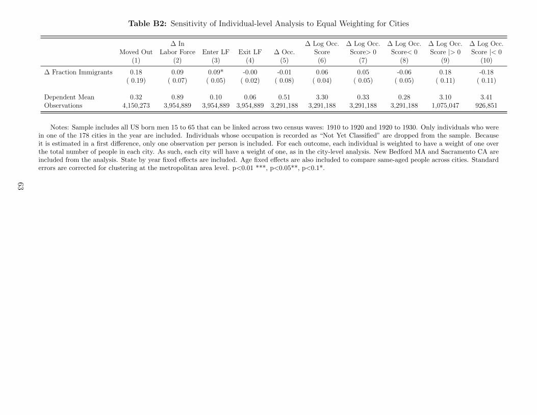
Table B2: Sensitivity of Individual-level Analysis to Equal Weighting for Cities

∆ In ∆ Log Occ. ∆ Log Occ. ∆ Log Occ. ∆ Log Occ. ∆ Log Occ.Moved Out Labor Force Enter LF Exit LF ∆ Occ. Score Score> 0 Score< 0 Score |> 0 Score |< 0

(1) (2) (3) (4) (5) (6) (7) (8) (9) (10)

∆ Fraction Immigrants 0.18 0.09 0.09* -0.00 -0.01 0.06 0.05 -0.06 0.18 -0.18( 0.19) ( 0.07) ( 0.05) ( 0.02) ( 0.08) ( 0.04) ( 0.05) ( 0.05) ( 0.11) ( 0.11)

Dependent Mean 0.32 0.89 0.10 0.06 0.51 3.30 0.33 0.28 3.10 3.41Observations 4,150,273 3,954,889 3,954,889 3,954,889 3,291,188 3,291,188 3,291,188 3,291,188 1,075,047 926,851

Notes: Sample includes all US born men 15 to 65 that can be linked across two census waves: 1910 to 1920 and 1920 to 1930. Only individuals who werein one of the 178 cities in the year are included. Individuals whose occupation is recorded as “Not Yet Classified” are dropped from the sample. Becauseit is estimated in a first difference, only one observation per person is included. For each outcome, each individual is weighted to have a weight of one overthe total number of people in each city. As such, each city will have a weight of one, as in the city-level analysis. New Bedford MA and Sacramento CA areincluded from the analysis. State by year fixed effects are included. Age fixed effects are also included to compare same-aged people across cities. Standarderrors are corrected for clustering at the metropolitan area level. p<0.01 ***, p<0.05**, p<0.1*.

63

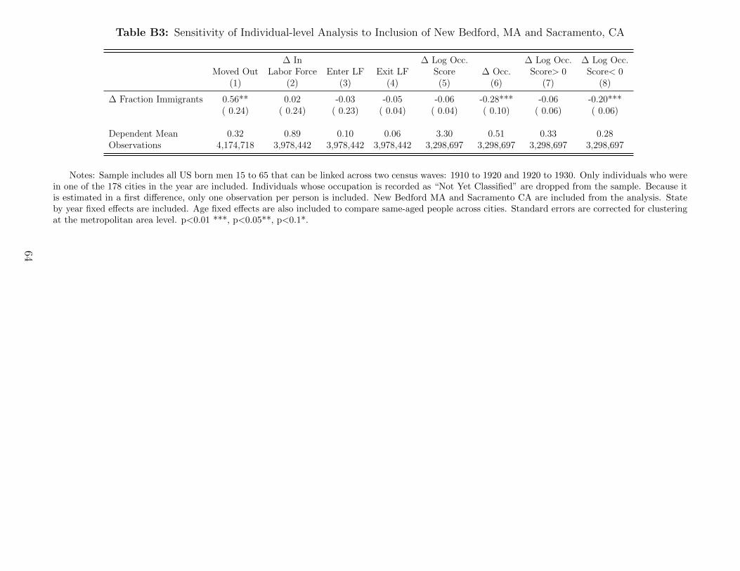
Table B3: Sensitivity of Individual-level Analysis to Inclusion of New Bedford, MA and Sacramento, CA

∆ In ∆ Log Occ. ∆ Log Occ. ∆ Log Occ.Moved Out Labor Force Enter LF Exit LF Score ∆ Occ. Score> 0 Score< 0

(1) (2) (3) (4) (5) (6) (7) (8)

∆ Fraction Immigrants 0.56** 0.02 -0.03 -0.05 -0.06 -0.28*** -0.06 -0.20***( 0.24) ( 0.24) ( 0.23) ( 0.04) ( 0.04) ( 0.10) ( 0.06) ( 0.06)

Dependent Mean 0.32 0.89 0.10 0.06 3.30 0.51 0.33 0.28Observations 4,174,718 3,978,442 3,978,442 3,978,442 3,298,697 3,298,697 3,298,697 3,298,697

Notes: Sample includes all US born men 15 to 65 that can be linked across two census waves: 1910 to 1920 and 1920 to 1930. Only individuals who werein one of the 178 cities in the year are included. Individuals whose occupation is recorded as “Not Yet Classified” are dropped from the sample. Because itis estimated in a first difference, only one observation per person is included. New Bedford MA and Sacramento CA are included from the analysis. Stateby year fixed effects are included. Age fixed effects are also included to compare same-aged people across cities. Standard errors are corrected for clusteringat the metropolitan area level. p<0.01 ***, p<0.05**, p<0.1*.

64

Table B4: Impact of Immigrant Flows on Economic Outcomes of US Born Men, WWI and Immigrant Quota Instruments


(1) (2) (3) (4) (5) (6) (7) (8)

∆ Fraction Immigrants 0.64*** 0.25*** 0.15*** -0.10*** -0.08** -0.17** -0.04 -0.12***( 0.23) ( 0.06) ( 0.04) ( 0.02) ( 0.03) ( 0.08) ( 0.04) ( 0.04)


Notes: Sample includes all US born men 15 to 65 that can be linked across two census waves: 1910 to 1920 and 1920 to 1930. Only individuals who werein one of the 178 cities in the year are included. Individuals whose occupation is recorded as “Not Yet Classified” are dropped from the sample. Because itis estimated in a first difference, only one observation per person is included. Following Tabellini (2020) New Bedford MA and Sacramento CA are excludedfrom the analysis. State by year fixed effects are included. Age fixed effects are not included. Standard errors are corrected for clustering at the metropolitanarea level. p<0.01 ***, p<0.05**, p<0.1*.

65

Table B5: Impact of Immigrant Flows on Economic Outcomes of US Born Men, Linked Individuals including Not Yet ClassifiedImputations


(1) (2) (3) (4) (5) (6) (7) (8)

∆ Fraction Immigrants 0.54** 0.21*** 0.15*** -0.06*** -0.05 -0.27*** -0.18*** -0.19***( 0.27) ( 0.05) ( 0.05) ( 0.02) ( 0.03) ( 0.07) ( 0.07) ( 0.05)


Notes: Sample includes all US born men 15 to 65 that can be linked across two census waves: 1910 to 1920 and 1920 to 1930. Only individuals who werein one of the 178 cities in the year are included. Individuals whose occupation is recorded as “Not Yet Classified” are assigned the average occ. score forindividuals their age in their state of residence. Because it is estimated in a first difference, only one observation per person is included. Following Tabellini(2020) New Bedford MA and Sacramento CA are excluded from the analysis. State by year fixed effects are included. Age fixed effects are also included tocompare same-aged people across cities. Standard errors are corrected for clustering at the metropolitan area level. p<0.01 ***, p<0.05**, p<0.1*.

66

Table B6: Robustness To Differential Trends by Pre-Period Characteristics, Individual Level

Predicted Value Added Skill Fraction Value of Emp. ShareBaseline Industrialization Manufacturing Ratios Black Products Manufacture

(1) (2) (3) (4) (5) (6) (7)

Outcome: Moved Out∆ Fraction Immigrants 0.57** 0.57** 0.60** 0.55** 0.57** 0.61** 0.59**

( 0.26) ( 0.25) ( 0.27) ( 0.25) ( 0.26) ( 0.28) ( 0.26)

Dependent Mean 0.32 0.32 0.33 0.32 0.32 0.33 0.33Observations 4,150,273 4,150,273 4,068,901 4,150,273 4,150,273 4,068,901 4,068,901

Outcome: ∆ Labor Force∆ Fraction Immigrants 0.22*** 0.22*** 0.22*** 0.25*** 0.24*** 0.21*** 0.22***

( 0.06) ( 0.05) ( 0.05) ( 0.06) ( 0.06) ( 0.06) ( 0.06)


Outcome: ∆ Log Occ. Score∆ Fraction Immigrants -0.06 -0.05 -0.08* -0.04 -0.06 -0.08* -0.07

( 0.05) ( 0.04) ( 0.05) ( 0.04) ( 0.05) ( 0.05) ( 0.05)


Notes: Sample includes all US born men 15 to 65 that can be linked across two census waves: 1910 to 1920 and 1920 to 1930. Only individuals who werein one of the 178 cities in the year are included. Individuals whose occupation is recorded as “Not Yet Classified” are assigned the average occ. score forindividuals their age in their state of residence. Because it is estimated in a first difference, only one observation per person is included. Following Tabellini(2020) New Bedford MA and Sacramento CA are excluded from the analysis. State by year fixed effects are included. Age fixed effects are also included tocompare same-aged people across cities. Standard errors are corrected for clustering at the metropolitan area level. p<0.01 ***, p<0.05**, p<0.1*.

67

Table B7: Robustness of Economics Effects To City and Immigrant Population Trends


(1) (2) (3) (4) (5) (6) (7) (8)

Control for City and Immigrant Size Quartiles (in 1900) Interacted with Cohort∆ Fraction Immigrants 0.08 0.11** 0.01 -0.10*** -0.00 -0.33*** -0.04 -0.22***

( 0.23) ( 0.05) ( 0.05) ( 0.03) ( 0.06) ( 0.11) ( 0.07) ( 0.07)


Notes: Sample includes all US born men 15 to 65 that can be linked across two census waves: 1910 to 1920 and 1920 to 1930. Only individuals who werein one of the 178 cities in the year are included. Individuals whose occupation is recorded as “Not Yet Classified” are dropped from the sample. Because itis estimated in a first difference, only one observation per person is included. Following Tabellini (2020) New Bedford MA and Sacramento CA are excludedfrom the analysis. State by year fixed effects are included. Age fixed effects are also included to compare same-aged people across cities. Standard errors arecorrected for clustering at the metropolitan area level. p<0.01 ***, p<0.05**, p<0.1*.

68

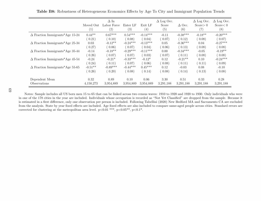
Table B8: Robustness of Heterogeneous Economics Effects by Age To City and Immigrant Population Trends


(1) (2) (3) (4) (5) (6) (7) (8)

∆ Fraction Immigrants*Age 15-24 0.44** 0.67*** 0.54*** -0.14*** -0.11 -0.38*** -0.18** -0.20***( 0.21) ( 0.10) ( 0.08) ( 0.04) ( 0.07) ( 0.12) ( 0.08) ( 0.07)

∆ Fraction Immigrants*Age 25-34 0.03 -0.12** -0.24*** -0.13*** 0.05 -0.36*** 0.04 -0.27***( 0.27) ( 0.06) ( 0.07) ( 0.04) ( 0.06) ( 0.13) ( 0.08) ( 0.08)

∆ Fraction Immigrants*Age 35-44 -0.14 -0.18** -0.29*** -0.11*** 0.00 -0.34*** -0.05 -0.19**( 0.26) ( 0.07) ( 0.07) ( 0.03) ( 0.07) ( 0.11) ( 0.08) ( 0.08)

∆ Fraction Immigrants*Age 45-54 -0.24 -0.21* -0.33*** -0.12* 0.12 -0.21** 0.10 -0.24***( 0.24) ( 0.11) ( 0.07) ( 0.06) ( 0.08) ( 0.11) ( 0.11) ( 0.09)

∆ Fraction Immigrants*Age 55-65 -0.51** -0.89*** -0.44*** 0.45*** 0.12 -0.03 0.08 -0.10( 0.26) ( 0.20) ( 0.08) ( 0.14) ( 0.08) ( 0.14) ( 0.13) ( 0.08)



69

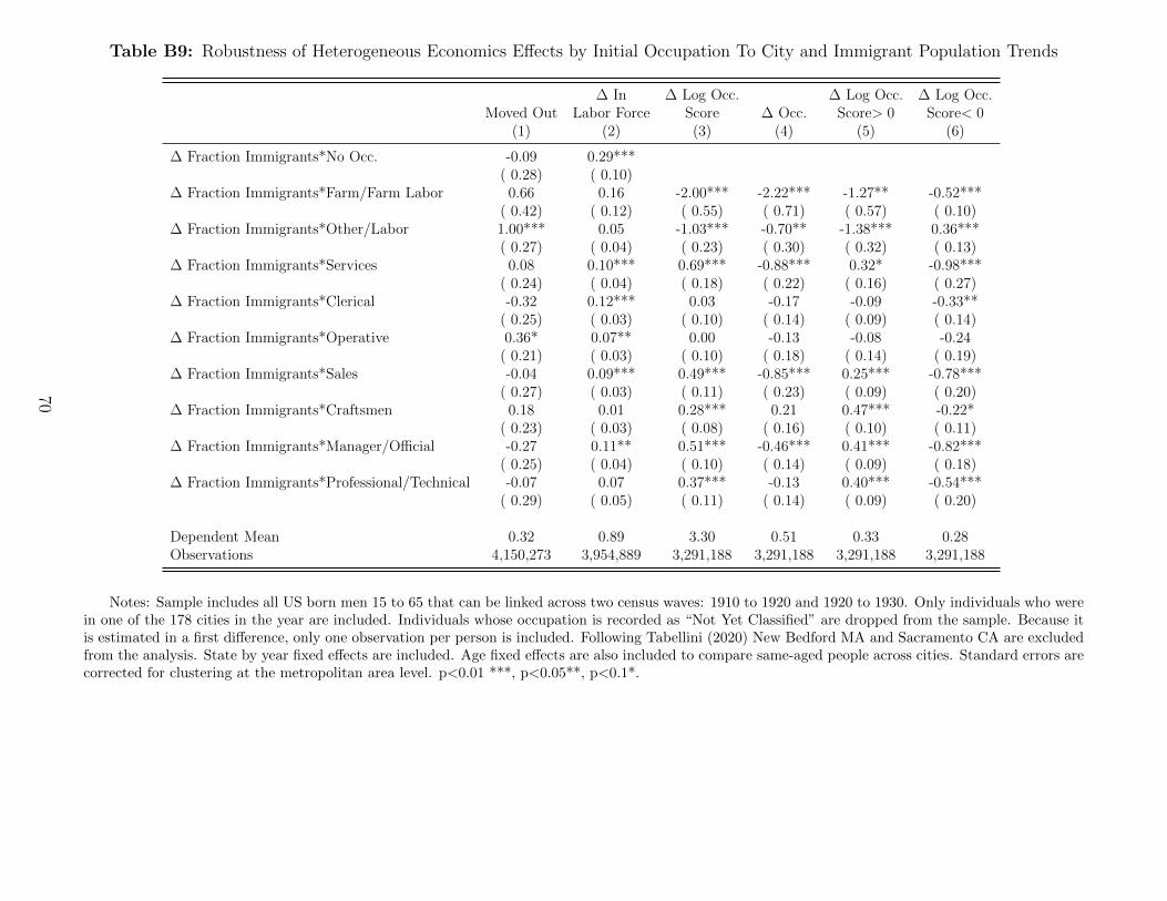
Table B9: Robustness of Heterogeneous Economics Effects by Initial Occupation To City and Immigrant Population Trends

∆ In ∆ Log Occ. ∆ Log Occ. ∆ Log Occ.Moved Out Labor Force Score ∆ Occ. Score> 0 Score< 0

(1) (2) (3) (4) (5) (6)

∆ Fraction Immigrants*No Occ. -0.09 0.29***( 0.28) ( 0.10)

∆ Fraction Immigrants*Farm/Farm Labor 0.66 0.16 -2.00*** -2.22*** -1.27** -0.52***( 0.42) ( 0.12) ( 0.55) ( 0.71) ( 0.57) ( 0.10)

∆ Fraction Immigrants*Other/Labor 1.00*** 0.05 -1.03*** -0.70** -1.38*** 0.36***( 0.27) ( 0.04) ( 0.23) ( 0.30) ( 0.32) ( 0.13)

∆ Fraction Immigrants*Services 0.08 0.10*** 0.69*** -0.88*** 0.32* -0.98***( 0.24) ( 0.04) ( 0.18) ( 0.22) ( 0.16) ( 0.27)

∆ Fraction Immigrants*Clerical -0.32 0.12*** 0.03 -0.17 -0.09 -0.33**( 0.25) ( 0.03) ( 0.10) ( 0.14) ( 0.09) ( 0.14)

∆ Fraction Immigrants*Operative 0.36* 0.07** 0.00 -0.13 -0.08 -0.24( 0.21) ( 0.03) ( 0.10) ( 0.18) ( 0.14) ( 0.19)

∆ Fraction Immigrants*Sales -0.04 0.09*** 0.49*** -0.85*** 0.25*** -0.78***( 0.27) ( 0.03) ( 0.11) ( 0.23) ( 0.09) ( 0.20)

∆ Fraction Immigrants*Craftsmen 0.18 0.01 0.28*** 0.21 0.47*** -0.22*( 0.23) ( 0.03) ( 0.08) ( 0.16) ( 0.10) ( 0.11)

∆ Fraction Immigrants*Manager/Official -0.27 0.11** 0.51*** -0.46*** 0.41*** -0.82***( 0.25) ( 0.04) ( 0.10) ( 0.14) ( 0.09) ( 0.18)

∆ Fraction Immigrants*Professional/Technical -0.07 0.07 0.37*** -0.13 0.40*** -0.54***( 0.29) ( 0.05) ( 0.11) ( 0.14) ( 0.09) ( 0.20)

Dependent Mean 0.32 0.89 3.30 0.51 0.33 0.28Observations 4,150,273 3,954,889 3,291,188 3,291,188 3,291,188 3,291,188


70

Table B10: Robustness of Heterogeneous Economics Effects by Mover-Status To City and Immigrant Population Trends

∆ In ∆ Log Occ. ∆ Log Occ. ∆ Log Occ.Labor Force Enter LF Exit LF Score ∆ Occ. Score> 0 Score< 0

(1) (2) (3) (4) (5) (6) (7)

∆ Fraction Immigrants*Stayer 0.06 0.01 -0.05* 0.13** -0.44*** 0.02 -0.39***( 0.06) ( 0.04) ( 0.03) ( 0.06) ( 0.11) ( 0.07) ( 0.07)

∆ Fraction Immigrants*Move-out 0.23*** 0.01 -0.22*** -0.32*** -0.09 -0.20** 0.17( 0.06) ( 0.07) ( 0.06) ( 0.12) ( 0.13) ( 0.10) ( 0.12)

Move-out 0.03** 0.00 -0.03** 0.01 -0.01 -0.00 -0.01( 0.01) ( 0.00) ( 0.01) ( 0.01) ( 0.01) ( 0.01) ( 0.01)



71

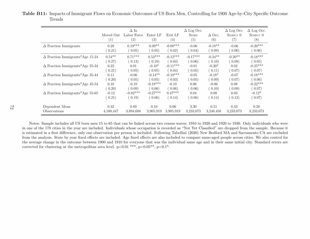
Table B11: Impacts of Immigrant Flows on Economic Outcomes of US Born Men, Controlling for 1900 Age-by-City Specific OutcomeTrends


(1) (2) (3) (4) (5) (6) (7) (8)

∆ Fraction Immigrants 0.28 0.19*** 0.09** -0.08*** -0.06 -0.18** -0.06 -0.20***( 0.21) ( 0.05) ( 0.05) ( 0.02) ( 0.04) ( 0.09) ( 0.06) ( 0.06)

∆ Fraction Immigrants*Age 15-24 0.54** 0.71*** 0.53*** -0.12*** -0.17*** -0.24** -0.20** -0.18***( 0.27) ( 0.13) ( 0.10) ( 0.04) ( 0.06) ( 0.10) ( 0.08) ( 0.05)

∆ Fraction Immigrants*Age 25-34 0.22 0.01 -0.10* -0.11*** -0.01 -0.20* 0.02 -0.25***( 0.21) ( 0.05) ( 0.05) ( 0.04) ( 0.05) ( 0.11) ( 0.07) ( 0.07)

∆ Fraction Immigrants*Age 35-44 0.11 -0.06 -0.14** -0.10*** -0.05 -0.18* -0.07 -0.18***( 0.20) ( 0.05) ( 0.05) ( 0.03) ( 0.05) ( 0.09) ( 0.07) ( 0.06)

∆ Fraction Immigrants*Age 45-54 0.10 -0.10 -0.18*** -0.10 0.06 -0.06 0.08 -0.22***( 0.20) ( 0.09) ( 0.06) ( 0.06) ( 0.06) ( 0.10) ( 0.09) ( 0.07)

∆ Fraction Immigrants*Age 55-65 -0.12 -0.82*** -0.27*** 0.47*** 0.04 0.08 0.03 -0.12*( 0.21) ( 0.19) ( 0.06) ( 0.14) ( 0.06) ( 0.14) ( 0.12) ( 0.07)


Notes: Sample includes all US born men 15 to 65 that can be linked across two census waves: 1910 to 1920 and 1920 to 1930. Only individuals who werein one of the 178 cities in the year are included. Individuals whose occupation is recorded as “Not Yet Classified” are dropped from the sample. Because itis estimated in a first difference, only one observation per person is included. Following Tabellini (2020) New Bedford MA and Sacramento CA are excludedfrom the analysis. State by year fixed effects are included. Age fixed effects are also included to compare same-aged people across cities. We also control forthe average change in the outcome between 1900 and 1910 for everyone that was the individual same age and in their same initial city. Standard errors arecorrected for clustering at the metropolitan area level. p<0.01 ***, p<0.05**, p<0.1*.

72

Table B12: Heterogeneous Impacts by Initial Occupation of Immigrant Flows on Economic Outcomes of US Born Men, Controllingfor 1900 Age-by-City Specific Outcome Trends

∆ In ∆ Log Occ. ∆ Log Occ. ∆ Log Occ.Moved Out Labor Force Score ∆ Occ. Score> 0 Score< 0

(1) (2) (3) (4) (5) (6)

∆ Fraction Immigrants*No Occ. 0.03 0.26***( 0.23) ( 0.10)

∆ Fraction Immigrants*Farm/Farm Labor 0.91** 0.12 -2.05*** -2.13*** -1.33** -0.50***( 0.39) ( 0.11) ( 0.56) ( 0.71) ( 0.57) ( 0.10)

∆ Fraction Immigrants*Other/Labor 1.20*** 0.02 -1.10*** -0.59* -1.42*** 0.37**( 0.30) ( 0.04) ( 0.26) ( 0.31) ( 0.33) ( 0.14)

∆ Fraction Immigrants*Services 0.27 0.08** 0.59*** -0.78*** 0.23 -0.95***( 0.20) ( 0.04) ( 0.16) ( 0.21) ( 0.16) ( 0.25)

∆ Fraction Immigrants*Clerical -0.20 0.09*** -0.06 -0.07 -0.15* -0.28**( 0.21) ( 0.03) ( 0.08) ( 0.12) ( 0.09) ( 0.12)

∆ Fraction Immigrants*Operative 0.54* 0.04 -0.09 -0.05 -0.16 -0.23( 0.28) ( 0.03) ( 0.11) ( 0.16) ( 0.15) ( 0.20)

∆ Fraction Immigrants*Sales 0.12 0.06** 0.39*** -0.73*** 0.17** -0.73***( 0.21) ( 0.03) ( 0.09) ( 0.22) ( 0.08) ( 0.18)

∆ Fraction Immigrants*Craftsmen 0.36* -0.02 0.19** 0.31** 0.39*** -0.18( 0.21) ( 0.04) ( 0.08) ( 0.15) ( 0.08) ( 0.13)

∆ Fraction Immigrants*Manager/Official -0.08 0.08* 0.41*** -0.35*** 0.33*** -0.77***( 0.20) ( 0.04) ( 0.08) ( 0.12) ( 0.07) ( 0.15)

∆ Fraction Immigrants*Professional/Technical 0.10 0.05 0.27*** -0.01 0.34*** -0.49***( 0.23) ( 0.04) ( 0.09) ( 0.12) ( 0.07) ( 0.17)

Dependent Mean 0.32 0.89 3.30 0.51 0.33 0.28Observations 4,100,447 3,894,688 3,233,073 3,248,458 3,233,073 3,233,073

Notes: Sample includes all US born men 15 to 65 that can be linked across two census waves: 1910 to 1920 and 1920 to 1930. Only individuals who werein one of the 178 cities in the year are included. Individuals whose occupation is recorded as “Not Yet Classified” are dropped from the sample. Because itis estimated in a first difference, only one observation per person is included. Following Tabellini (2020) New Bedford MA and Sacramento CA are excludedfrom the analysis. State by year fixed effects are included. Age fixed effects are also included to compare same-aged people across cities. We also control forthe average change in the outcome between 1900 and 1910 for everyone that was the individual same age and in their same initial city. “Not Yet Classified”occupations are occupation strings that occur rarely in the original Census files and have not been classified into an occupation yet. Standard errors arecorrected for clustering at the metropolitan area level. p<0.01 ***, p<0.05**, p<0.1*.

73

Table B13: Heterogeneous Impacts by Migration Status of Immigrant Flows on Economic Outcomes of US Born Men, Controllingfor 1900 Age-by-City Specific Outcome Trends


(1) (2) (3) (4) (5) (6) (7)

∆ Fraction Immigrants*Stayer 0.14** 0.08* -0.05 0.11** -0.39*** -0.01 -0.44***( 0.06) ( 0.04) ( 0.03) ( 0.05) ( 0.09) ( 0.07) ( 0.07)

∆ Fraction Immigrants*Move-out 0.32*** 0.09* -0.21*** -0.32*** -0.06 -0.22** 0.11( 0.07) ( 0.05) ( 0.05) ( 0.11) ( 0.13) ( 0.09) ( 0.13)

Move-out -0.00 0.01*** 0.02*** -0.11*** 0.21*** 0.02*** 0.18***( 0.00) ( 0.00) ( 0.00) ( 0.01) ( 0.01) ( 0.01) ( 0.01)


Notes: Sample includes all US born men 15 to 65 that can be linked across two census waves: 1910 to 1920 and 1920 to 1930. Only individuals who werein one of the 178 cities in the year are included. Individuals whose occupation is recorded as “Not Yet Classified” are dropped from the sample. Because itis estimated in a first difference, only one observation per person is included. Following Tabellini (2020) New Bedford MA and Sacramento CA are excludedfrom the analysis. State by year fixed effects are included. Age fixed effects are also included to compare same-aged people across cities. We also control forthe average change in the outcome between 1900 and 1910 for everyone that was the individual same age and in their same initial city. “Not Yet Classified”occupations are occupation strings that occur rarely in the original Census files and have not been classified into an occupation yet. Standard errors arecorrected for clustering at the metropolitan area level. p<0.01 ***, p<0.05**, p<0.1*.

74

Table C1: First Stage Relationship Between Immigration Instruments and Fraction Immigrants

City-Level Individual LevelFraction

Immigrants ∆ Fraction Immigrants ∆ Fraction Immigrants(1) (2) (3) (4) (5) (6) (7) (8) (9)

Immig. Shift Share 0.99 ***( 0.07)

∆ Immig. Shift Share 0.93*** 0.85***( 0.09) ( 0.06)

Quota*1920 1.08*** 0.46 0.78*** 0.32( 0.21) ( 0.42) ( 0.19) ( 0.28)

Quota*1930 0.24* 0.77** 0.30 0.78**( 0.13) ( 0.35) ( 0.22) ( 0.31)

WWI*1920 0.64*** 0.77*** 0.88*** 0.70*** 0.83*** 0.91***( 0.07) ( 0.11) ( 0.06) ( 0.09) ( 0.10) ( 0.06)

WWI*1930 0.18*** 0.06 0.24*** 0.03 -0.10 0.11( 0.04) ( 0.08) ( 0.03) ( 0.08) ( 0.11) ( 0.07)

New Bedford/Sacramento X XF-Statistic 217.32 101.07 102.19 106.84 192.62 236.71 73.08 75.03 128.95Dependent Mean 0.04 -0.03 -0.03 -0.03 -0.03 -0.03 -0.03 -0.03 -0.03Observations 534 356 356 360 356 4,150,273 4,150,273 4,174,718 4,150,273

Notes: Sample includes all US born men 15 to 65 from 1910, 1920, or 1930. Only individuals who were in one of the 178 cities in the year are included.Individuals whose occupation is recorded as “Not Yet Classified” are dropped from the sample. Following Tabellini (2020) New Bedford MA and SacramentoCA are excluded from all columns but (4) and (8). State by year fixed effects are included. Age fixed effects are not included. Standard errors are correctedfor clustering at the metropolitan area level. p<0.01 ***, p<0.05**, p<0.1*.

75

Table C2: Importance of Age Fixed Effects: Impact of Immigrant Flows on Economic Outcomes of US Born Men, Linked Individuals


(1) (2) (3) (4) (5) (6) (7) (8)

∆ Fraction Immigrants 0.51** -0.33*** -0.24*** 0.09** -0.24*** -0.57*** -0.40*** -0.20***( 0.25) ( 0.07) ( 0.06) ( 0.04) ( 0.05) ( 0.11) ( 0.08) ( 0.06)



76

Table C3: Impact of Immigrant Flows on Economic Outcomes of US Born Women, Linked Individuals


(1) (2) (3) (4) (5) (6) (7) (8)

∆ Fraction Immigrants 0.52* 0.21*** 0.11** -0.10 -0.00 -0.12 -0.29** -0.11( 0.27) ( 0.06) ( 0.04) ( 0.07) ( 0.09) ( 0.15) ( 0.14) ( 0.07)

Dependent Mean 0.30 0.20 0.10 0.10 2.88 0.35 0.26 0.23Observations 5,991,226 5,810,230 5,810,230 5,810,230 577,898 577,898 577,898 577,898

Notes: Sample includes all US born women 15 to 65 that can be linked across two census waves: 1910 to 1920 and 1920 to 1930. Only individualswho were in one of the 178 cities in the year are included. Individuals whose occupation is recorded as “Not Yet Classified” are dropped from the sample.Because it is estimated in a first difference, only one observation per person is included. Following Tabellini (2020) New Bedford MA and Sacramento CA areexcluded from the analysis. State by year fixed effects are included. Age fixed effects are also included to compare same-aged people across cities. Standarderrors are corrected for clustering at the metropolitan area level. p<0.01 ***, p<0.05**, p<0.1*.

77

Table C4: Heterogeneous Impact by Migration Status of Immigrant Flows on Economic Outcomes of US Born Women, LinkedIndividuals


(1) (2) (3) (4) (5) (6) (7)

∆ Fraction Immigrants*Stayer 0.22*** 0.09* -0.13* 0.09 -0.32** -0.35** -0.23***( 0.07) ( 0.05) ( 0.07) ( 0.08) ( 0.16) ( 0.14) ( 0.09)

∆ Fraction Immigrants*Move-out 0.34*** 0.16*** -0.18* -0.24 0.04 -0.35* -0.04( 0.11) ( 0.05) ( 0.09) ( 0.19) ( 0.16) ( 0.19) ( 0.09)

Move-out -0.07*** 0.00*** 0.08*** -0.03*** 0.29*** 0.13*** 0.16***( 0.00) ( 0.00) ( 0.00) ( 0.01) ( 0.01) ( 0.00) ( 0.01)

Dependent Mean 0.20 0.10 0.10 2.88 0.35 0.26 0.23Observations 5,810,230 5,810,230 5,810,230 577,898 577,898 577,898 577,898

Notes: Sample includes all US born women 15 to 65 that can be linked across two census waves: 1910 to 1920 and 1920 to 1930. Only individualswho were in one of the 178 cities in the year are included. Individuals whose occupation is recorded as “Not Yet Classified” are dropped from the sample.Because it is estimated in a first difference, only one observation per person is included. Following Tabellini (2020) New Bedford MA and Sacramento CA areexcluded from the analysis. State by year fixed effects are included. Age fixed effects are also included to compare same-aged people across cities. Standarderrors are corrected for clustering at the metropolitan area level. p<0.01 ***, p<0.05**, p<0.1*.

78

Table C5: City-level Impact of Immigrant Flows on Family Formation Outcomes ofUS Born Men

Linkable Following(1) (2)

∆ MarriedFraction Immigrants 0.19*** 0.28***

( 0.06) ( 0.05)

Dependent Mean (in levels) 0.57 0.60Observations 356 356

∆ Never MarriedFraction Immigrants -0.24*** -0.34***

( 0.07) ( 0.05)


∆ DivorcedFraction Immigrants 0.00 0.01*

( 0.00) ( 0.00)


Notes: Observation at the city level for 1910, 1920, or 1930 for 178 cities that had a populationover 30,000 in each census year. Only US born men 15-65 in the initial census wave are included.Individuals whose occupation is recorded as “Not Yet Classified” are dropped from the sample.Following Tabellini (2020) New Bedford MA and Sacramento CA are excluded from the analysis.The “Tabellini” specifications use both the data and specification used by Tabellini (2020). The“Linkable” specifications construct city level measures from individuals that can be linked from onecensus wave to the next in the Ancestry version of the full count census. In the levels specificationscity and state by year fixed effects are included. In the first difference specifications state by yearfixed effects are included. Standard errors are corrected for clustering at the metropolitan area level.p<0.01 ***, p<0.05**, p<0.1*.

79

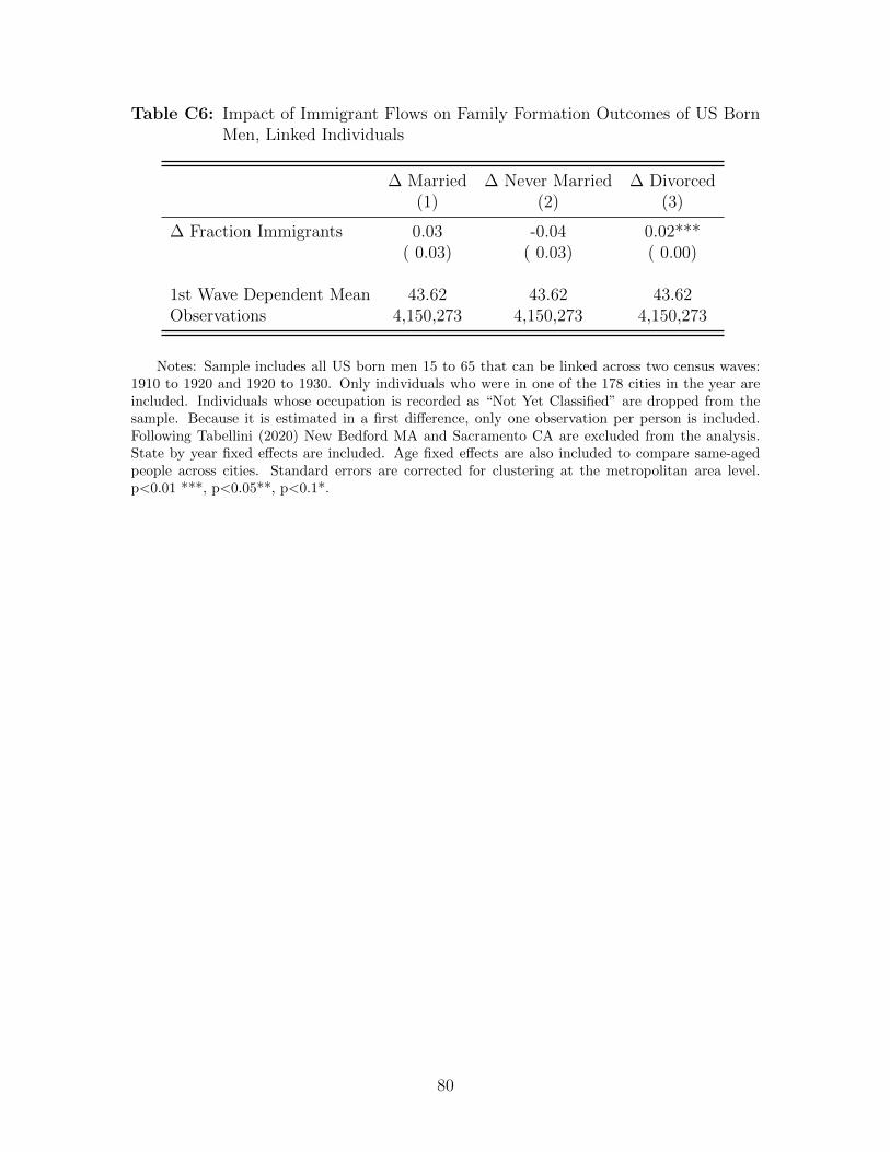
Table C6: Impact of Immigrant Flows on Family Formation Outcomes of US BornMen, Linked Individuals

∆ Married ∆ Never Married ∆ Divorced(1) (2) (3)

∆ Fraction Immigrants 0.03 -0.04 0.02***( 0.03) ( 0.03) ( 0.00)

1st Wave Dependent Mean 43.62 43.62 43.62Observations 4,150,273 4,150,273 4,150,273

Notes: Sample includes all US born men 15 to 65 that can be linked across two census waves:1910 to 1920 and 1920 to 1930. Only individuals who were in one of the 178 cities in the year areincluded. Individuals whose occupation is recorded as “Not Yet Classified” are dropped from thesample. Because it is estimated in a first difference, only one observation per person is included.Following Tabellini (2020) New Bedford MA and Sacramento CA are excluded from the analysis.State by year fixed effects are included. Age fixed effects are also included to compare same-agedpeople across cities. Standard errors are corrected for clustering at the metropolitan area level.p<0.01 ***, p<0.05**, p<0.1*.

80

Table C7: Impact of Immigrant Flows on Family Formation Outcomes of Young USBorn Men, Linked Individuals

Married Never Married Divorced(1) (2) (3)

∆ Fraction Immigrants 0.38*** -0.37*** 0.00**( 0.11) ( 0.12) ( 0.00)

Dependent Mean 44.27 44.27 44.27Observations 2,253,490 2,253,490 2,253,490

Notes: Sample includes all US born men 5 to 14 in the initial wave that can be linked across twocensus waves: 1910 to 1920 and 1920 to 1930. Only individuals who were in one of the 178 cities inthe year are included. Individuals whose occupation is recorded as “Not Yet Classified” are droppedfrom the sample. Because it is estimated in a first difference, only one observation per person isincluded. Following Tabellini (2020) New Bedford MA and Sacramento CA are excluded from theanalysis. State by year fixed effects are included. Age fixed effects are also included to comparesame-aged people across cities. Standard errors are corrected for clustering at the metropolitan arealevel. p<0.01 ***, p<0.05**, p<0.1*.

81

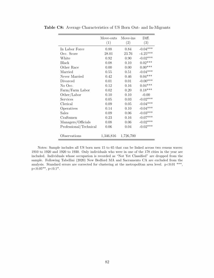
Table C8: Average Characteristics of US Born Out- and In-Migrants

Move-outs Move-ins Diff.(1) (2) (3)

In Labor Force 0.88 0.84 -0.04***Occ. Score 28.01 23.76 -4.25***White 0.92 0.90 -0.02***Black 0.08 0.10 0.02***Other Race 0.00 0.00 0.00***Married 0.55 0.51 -0.04***Never Married 0.42 0.46 0.04***Divorced 0.01 0.01 -0.00***No Occ. 0.12 0.16 0.04***Farm/Farm Labor 0.02 0.20 0.18***Other/Labor 0.10 0.10 -0.00Services 0.05 0.03 -0.02***Clerical 0.09 0.05 -0.04***Operatives 0.14 0.10 -0.04***Sales 0.09 0.06 -0.03***Craftsmen 0.23 0.16 -0.07***Managers/Officials 0.08 0.06 -0.02***Professional/Technical 0.06 0.04 -0.02***

Observations 1,346,816 1,726,700

Notes: Sample includes all US born men 15 to 65 that can be linked across two census waves:1910 to 1920 and 1920 to 1930. Only individuals who were in one of the 178 cities in the year areincluded. Individuals whose occupation is recorded as “Not Yet Classified” are dropped from thesample. Following Tabellini (2020) New Bedford MA and Sacramento CA are excluded from theanalysis. Standard errors are corrected for clustering at the metropolitan area level. p<0.01 ***,p<0.05**, p<0.1*.

82

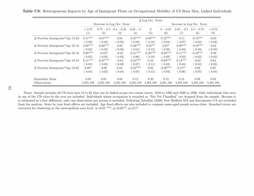
Table C9: Heterogeneous Impacts by Age of Immigrant Flows on Occupational Mobility of US Born Men, Linked Individuals

∆ Log Occ. ScoreDecrease in Log Occ. Score Increase in Log Occ. Score

> 0.75 0.75− 0.5 0.5− 0.25 0.25− 0 0 0− 0.25 0.25− 0.5 0.5− 0.75 > 0.75(1) (2) (3) (4) (5) (6) (7) (8) (9)

∆ Fraction Immigrants*Age 15-24 0.11*** -0.07*** 0.04 -0.27*** 0.40*** 0.12*** -0.11 -0.19*** -0.03( 0.02) ( 0.02) ( 0.03) ( 0.04) ( 0.10) ( 0.04) ( 0.07) ( 0.04) ( 0.04)

∆ Fraction Immigrants*Age 25-34 0.06*** -0.08*** 0.02 -0.26*** 0.25** 0.05* 0.09*** -0.10*** -0.02( 0.02) ( 0.02) ( 0.03) ( 0.04) ( 0.12) ( 0.03) ( 0.03) ( 0.03) ( 0.03)

∆ Fraction Immigrants*Age 35-44 0.08*** -0.03* -0.02 -0.21*** 0.26*** -0.08*** 0.11*** -0.10*** -0.00( 0.02) ( 0.02) ( 0.03) ( 0.06) ( 0.10) ( 0.03) ( 0.03) ( 0.03) ( 0.03)

∆ Fraction Immigrants*Age 45-54 0.11*** -0.07*** -0.04 -0.24*** 0.16 -0.09*** 0.14*** -0.02 0.04( 0.03) ( 0.02) ( 0.03) ( 0.07) ( 0.11) ( 0.03) ( 0.04) ( 0.04) ( 0.03)

∆ Fraction Immigrants*Age 55-65 0.08* -0.00 0.04 -0.22*** 0.05 -0.20*** 0.15** 0.06 0.05( 0.04) ( 0.03) ( 0.04) ( 0.05) ( 0.15) ( 0.04) ( 0.06) ( 0.05) ( 0.04)

Dependent Mean 0.03 0.05 0.08 0.12 0.39 0.13 0.10 0.08 0.03Observations 3,291,188 3,291,188 3,291,188 3,291,188 3,291,188 3,291,188 3,291,188 3,291,188 3,291,188


83

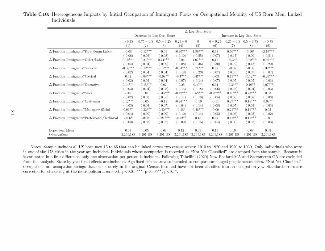
Table C10: Heterogeneous Impacts by Initial Occupation of Immigrant Flows on Occupational Mobility of US Born Men, LinkedIndividuals

∆ Log Occ. ScoreDecrease in Log Occ. Score Increase in Log Occ. Score

> 0.75 0.75− 0.5 0.5− 0.25 0.25− 0 0 0− 0.25 0.25− 0.5 0.5− 0.75 > 0.75(1) (2) (3) (4) (5) (6) (7) (8) (9)

∆ Fraction Immigrants*Farm/Farm Labor -0.08 -0.12*** -0.01 -0.30*** 1.86*** 0.03 0.66*** 0.16* -2.19***( 0.06) ( 0.03) ( 0.08) ( 0.10) ( 0.55) ( 0.07) ( 0.13) ( 0.09) ( 0.51)

∆ Fraction Immigrants*Other/Labor 0.19*** -0.21*** 0.44*** -0.04 1.07*** 0.15 -0.35* -0.70*** -0.56***( 0.04) ( 0.04) ( 0.09) ( 0.08) ( 0.36) ( 0.30) ( 0.19) ( 0.13) ( 0.20)

∆ Fraction Immigrants*Services -0.08*** -0.12*** -0.12*** -0.64*** 0.71*** 0.07 -0.07 -0.08 0.32***( 0.02) ( 0.04) ( 0.04) ( 0.18) ( 0.23) ( 0.07) ( 0.10) ( 0.07) ( 0.07)

∆ Fraction Immigrants*Clerical 0.02 -0.08*** -0.08** -0.17** 0.47*** -0.03 0.19*** -0.12** -0.20***( 0.02) ( 0.02) ( 0.04) ( 0.07) ( 0.14) ( 0.07) ( 0.05) ( 0.05) ( 0.03)

∆ Fraction Immigrants*Operative 0.14*** -0.15*** 0.02 -0.25 0.40** 0.01 -0.34** 0.10** 0.07***( 0.03) ( 0.04) ( 0.08) ( 0.15) ( 0.18) ( 0.06) ( 0.16) ( 0.04) ( 0.03)

∆ Fraction Immigrants*Sales -0.01 0.01 -0.33*** -0.42*** 0.58*** -0.23*** 0.16*** 0.23*** 0.03( 0.02) ( 0.03) ( 0.05) ( 0.11) ( 0.18) ( 0.05) ( 0.05) ( 0.08) ( 0.03)

∆ Fraction Immigrants*Craftsmen 0.12*** 0.05 -0.11 -0.26*** -0.19 -0.11 0.27*** 0.15*** 0.08**( 0.03) ( 0.04) ( 0.07) ( 0.04) ( 0.14) ( 0.08) ( 0.05) ( 0.03) ( 0.03)

∆ Fraction Immigrants*Manager/Official 0.09** -0.32*** -0.40*** -0.18* 0.46*** -0.00 0.21*** 0.11*** 0.03( 0.04) ( 0.09) ( 0.09) ( 0.10) ( 0.14) ( 0.05) ( 0.05) ( 0.03) ( 0.02)

∆ Fraction Immigrants*Professional/Technical -0.06* -0.03 -0.21*** -0.22** 0.18 0.07 0.17*** 0.11*** -0.01( 0.03) ( 0.03) ( 0.07) ( 0.09) ( 0.15) ( 0.04) ( 0.06) ( 0.03) ( 0.03)

Dependent Mean 0.03 0.05 0.08 0.12 0.39 0.13 0.10 0.08 0.03Observations 3,291,188 3,291,188 3,291,188 3,291,188 3,291,188 3,291,188 3,291,188 3,291,188 3,291,188

Notes: Sample includes all US born men 15 to 65 that can be linked across two census waves: 1910 to 1920 and 1920 to 1930. Only individuals who werein one of the 178 cities in the year are included. Individuals whose occupation is recorded as “Not Yet Classified” are dropped from the sample. Because itis estimated in a first difference, only one observation per person is included. Following Tabellini (2020) New Bedford MA and Sacramento CA are excludedfrom the analysis. State by year fixed effects are included. Age fixed effects are also included to compare same-aged people across cities. “Not Yet Classified”occupations are occupation strings that occur rarely in the original Census files and have not been classified into an occupation yet. Standard errors arecorrected for clustering at the metropolitan area level. p<0.01 ***, p<0.05**, p<0.1*.

84

Table C11: Impact of Immigrant Flows on Economic Outcomes of US Born Men, OLS


(1) (2) (3) (4) (5) (6) (7) (8)

∆ Fraction Immigrants -0.14 0.15*** 0.11*** -0.03** 0.02 -0.21*** -0.06 -0.11**( 0.19) ( 0.03) ( 0.03) ( 0.02) ( 0.04) ( 0.08) ( 0.08) ( 0.05)



85

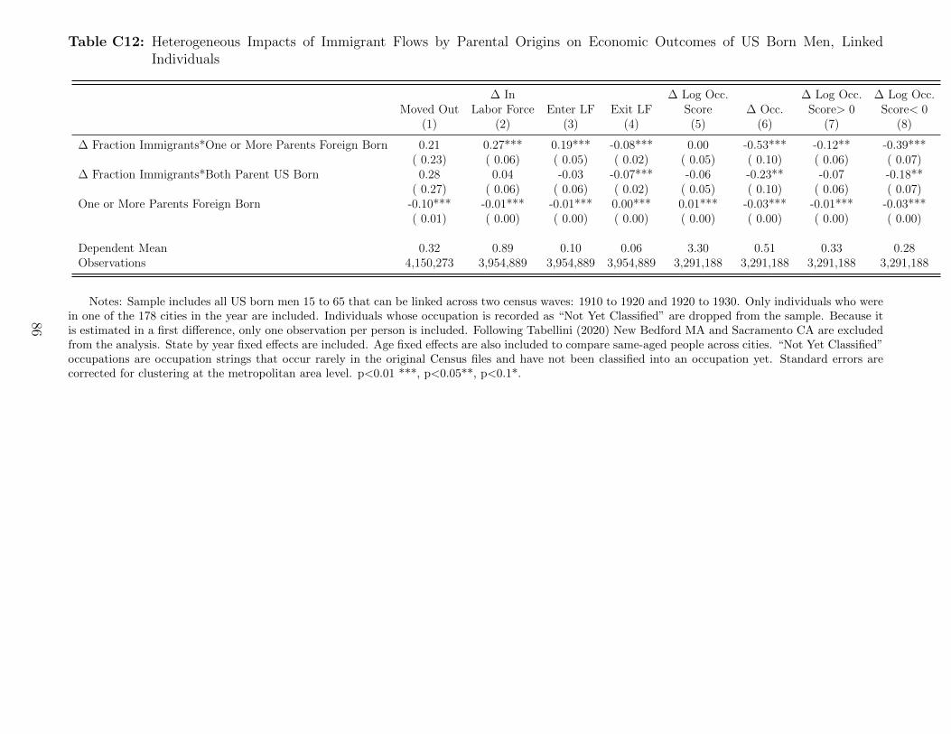
Table C12: Heterogeneous Impacts of Immigrant Flows by Parental Origins on Economic Outcomes of US Born Men, LinkedIndividuals


(1) (2) (3) (4) (5) (6) (7) (8)

∆ Fraction Immigrants*One or More Parents Foreign Born 0.21 0.27*** 0.19*** -0.08*** 0.00 -0.53*** -0.12** -0.39***( 0.23) ( 0.06) ( 0.05) ( 0.02) ( 0.05) ( 0.10) ( 0.06) ( 0.07)

∆ Fraction Immigrants*Both Parent US Born 0.28 0.04 -0.03 -0.07*** -0.06 -0.23** -0.07 -0.18**( 0.27) ( 0.06) ( 0.06) ( 0.02) ( 0.05) ( 0.10) ( 0.06) ( 0.07)

One or More Parents Foreign Born -0.10*** -0.01*** -0.01*** 0.00*** 0.01*** -0.03*** -0.01*** -0.03***( 0.01) ( 0.00) ( 0.00) ( 0.00) ( 0.00) ( 0.00) ( 0.00) ( 0.00)


Notes: Sample includes all US born men 15 to 65 that can be linked across two census waves: 1910 to 1920 and 1920 to 1930. Only individuals who werein one of the 178 cities in the year are included. Individuals whose occupation is recorded as “Not Yet Classified” are dropped from the sample. Because itis estimated in a first difference, only one observation per person is included. Following Tabellini (2020) New Bedford MA and Sacramento CA are excludedfrom the analysis. State by year fixed effects are included. Age fixed effects are also included to compare same-aged people across cities. “Not Yet Classified”occupations are occupation strings that occur rarely in the original Census files and have not been classified into an occupation yet. Standard errors arecorrected for clustering at the metropolitan area level. p<0.01 ***, p<0.05**, p<0.1*.

86

Table C13: Heterogeneous Impacts of Immigrant Flows by Age and Parental Origins on Economic Outcomes of US Born Men,Linked Individuals


(1) (2) (3) (4) (5) (6) (7) (8)

∆ Fraction Immigrants*One or More Parent 0.20 0.82*** 0.67*** -0.15*** -0.11* -0.47*** -0.17** -0.35***Foregin Born*Age 15-24 ( 0.26) ( 0.17) ( 0.15) ( 0.04) ( 0.06) ( 0.10) ( 0.08) ( 0.06)∆ Fraction Immigrants*One or More Parent 0.23 -0.01 -0.12** -0.11*** 0.09** -0.56*** -0.00 -0.45***Foregin Born*Age 25-34 ( 0.23) ( 0.05) ( 0.06) ( 0.03) ( 0.04) ( 0.13) ( 0.07) ( 0.09)∆ Fraction Immigrants*One or More Parent 0.14 -0.06 -0.17*** -0.12*** -0.02 -0.60*** -0.18*** -0.36***Foregin Born*Age 35-44 ( 0.22) ( 0.06) ( 0.05) ( 0.03) ( 0.05) ( 0.10) ( 0.06) ( 0.06)∆ Fraction Immigrants*One or More Parent 0.11 -0.15 -0.20*** -0.05 0.08 -0.59*** -0.12* -0.43***Foregin Born*Age 45-54 ( 0.24) ( 0.10) ( 0.06) ( 0.06) ( 0.06) ( 0.10) ( 0.07) ( 0.10)∆ Fraction Immigrants*One or More Parent -0.10 -0.86*** -0.36*** 0.51*** 0.08 -0.46** -0.17 -0.37***Foregin Born*Age 55-65 ( 0.27) ( 0.16) ( 0.07) ( 0.11) ( 0.09) ( 0.18) ( 0.15) ( 0.10)∆ Fraction Immigrants*Both Parents 0.81*** 0.36*** 0.27** -0.10** -0.20*** -0.42*** -0.28*** -0.21***US Born*Age 15-24 ( 0.29) ( 0.11) ( 0.11) ( 0.04) ( 0.07) ( 0.12) ( 0.09) ( 0.07)∆ Fraction Immigrants*Both Parents 0.11 0.01 -0.13** -0.13*** -0.05 -0.32*** -0.05 -0.24***US Born*Age 25-34 ( 0.32) ( 0.06) ( 0.06) ( 0.04) ( 0.06) ( 0.11) ( 0.08) ( 0.08)∆ Fraction Immigrants*Both Parents -0.00 -0.07 -0.16*** -0.08*** -0.04 -0.19* -0.06 -0.11US Born*Age 35-44 ( 0.28) ( 0.06) ( 0.06) ( 0.03) ( 0.06) ( 0.10) ( 0.07) ( 0.09)∆ Fraction Immigrants*Both Parents 0.02 -0.10 -0.19*** -0.08 0.09 0.08 0.21** -0.13US Born*Age 45-54 ( 0.25) ( 0.10) ( 0.06) ( 0.07) ( 0.07) ( 0.11) ( 0.10) ( 0.09)∆ Fraction Immigrants*Both Parents -0.00 -0.76*** -0.25*** 0.50*** 0.08 0.26* 0.20* 0.04US Born*Age 55-65 ( 0.26) ( 0.20) ( 0.06) ( 0.17) ( 0.07) ( 0.14) ( 0.10) ( 0.08)


Notes: Sample includes all US born men 15 to 65 that can be linked across two census waves: 1910 to 1920 and 1920 to 1930. Only individuals who werein one of the 178 cities in the year are included. Individuals whose occupation is recorded as “Not Yet Classified” are dropped from the sample. Because itis estimated in a first difference, only one observation per person is included. Following Tabellini (2020) New Bedford MA and Sacramento CA are excludedfrom the analysis. State by year fixed effects are included. Age fixed effects are also included to compare same-aged people across cities. The indicator forhaving at least one foreign born parent interacted with age fixed effects are also included. “Not Yet Classified” occupations are occupation strings that occurrarely in the original Census files and have not been classified into an occupation yet. Standard errors are corrected for clustering at the metropolitan arealevel. p<0.01 ***, p<0.05**, p<0.1*.

87

Table C14: Heterogeneous Impacts of Immigrant Flows by Migration Status and Parental Origins on Economic Outcomes of USBorn Men, Linked Individuals


(1) (2) (3) (4) (5) (6) (7)

∆ Fraction Immigrants*Stayer*One or More Parent 0.21*** 0.15*** -0.06* 0.08 -0.64*** -0.12* -0.51***Foreign Born ( 0.06) ( 0.05) ( 0.03) ( 0.05) ( 0.11) ( 0.07) ( 0.07)∆ Fraction Immigrants*Move-out*One or More Parent 0.42*** 0.28*** -0.14*** -0.21* -0.31** -0.16* -0.08Foreign Born ( 0.08) ( 0.06) ( 0.04) ( 0.12) ( 0.14) ( 0.09) ( 0.14)∆ Fraction Immigrants*Stayer*Both Parents -0.03 -0.02 0.01 0.10* -0.36*** 0.02 -0.39***US Born ( 0.07) ( 0.05) ( 0.03) ( 0.06) ( 0.11) ( 0.07) ( 0.07)∆ Fraction Immigrants*Move-out*Both Parents 0.19*** -0.05 -0.24*** -0.30*** -0.16 -0.25*** 0.10US Born ( 0.07) ( 0.07) ( 0.05) ( 0.11) ( 0.13) ( 0.09) ( 0.14)Move-out -0.00 0.01*** 0.01*** -0.12*** 0.21*** 0.01*** 0.19***

( 0.00) ( 0.00) ( 0.00) ( 0.01) ( 0.00) ( 0.01) ( 0.01)Move-out*One or More Parents Foreign Born -0.01*** -0.00 0.01*** 0.02*** -0.02*** 0.01* -0.03***

( 0.00) ( 0.00) ( 0.00) ( 0.01) ( 0.01) ( 0.01) ( 0.01)Move-out*Both Parents US Born -0.01*** -0.01*** 0.01*** -0.01*** -0.01** -0.02*** -0.00

( 0.00) ( 0.00) ( 0.00) ( 0.00) ( 0.00) ( 0.00) ( 0.00)


Notes: Sample includes all US born men 15 to 65 that can be linked across two census waves: 1910 to 1920 and 1920 to 1930. Only individuals who werein one of the 178 cities in the year are included. Individuals whose occupation is recorded as “Not Yet Classified” are dropped from the sample. Because itis estimated in a first difference, only one observation per person is included. Following Tabellini (2020) New Bedford MA and Sacramento CA are excludedfrom the analysis. State by year fixed effects are included. Age fixed effects are also included to compare same-aged people across cities. The indicator forhaving at least one foreign born parent interacted with age fixed effects are also included. “Not Yet Classified” occupations are occupation strings that occurrarely in the original Census files and have not been classified into an occupation yet. Standard errors are corrected for clustering at the metropolitan arealevel. p<0.01 ***, p<0.05**, p<0.1*.

88

Table C15: Heterogeneous Impacts of Immigrant Flows by Initial Status on Economic Outcomes of US Born Men, Linked Individuals

∆ In ∆ InMoved Out Labor Force Moved Out Labor Force

(1) (2) (3) (4)

∆ Fraction Immigrants*Initially In L.F. 0.53** 0.02 0.54** 0.02( 0.25) ( 0.03) ( 0.25) ( 0.03)

∆ Fraction Immigrants*Initially Out L.F. 0.65** 0.98*** 0.62** 1.08***( 0.29) ( 0.27) ( 0.29) ( 0.24)

∆ Fraction Immigrants*Initially In School 0.89*** 0.15* 0.83*** 0.13( 0.29) ( 0.08) ( 0.28) ( 0.08)

Initial Status*Age Fixed Effects X XDependent Mean 0.32 0.89 0.32 0.89Observations 4,032,953 3,954,547 4,032,953 3,954,547

Notes: Sample includes all US born men 15 to 65 that can be linked across two census waves: 1910 to 1920 and 1920 to 1930. Only individuals who werein one of the 178 cities in the year are included. Individuals whose occupation is recorded as “Not Yet Classified” are dropped from the sample. Because itis estimated in a first difference, only one observation per person is included. Following Tabellini (2020) New Bedford MA and Sacramento CA are excludedfrom the analysis. State by year fixed effects are included. In columns (1) and (2) age fixed effects interacted with first wave status student, out of laborforce, in labor force) are also included to compare same-aged, same-status people across cities as well as indicators for being a student or not in the laborforce in the first wave. In columns (3) and (4) age fixed effects interacted with first wave status (student, out of labor force, in labor force) are also includedto compare same-aged, same-status people across cities. “Not Yet Classified” occupations are occupation strings that occur rarely in the original Censusfiles and have not been classified into an occupation yet. Standard errors are corrected for clustering at the metropolitan area level. p<0.01 ***, p<0.05**,p<0.1*.

89

Table C16: Heterogeneous Impacts by Race of Immigrant Flows on Economic Outcomes of US Born Men, Linked Individuals


(1) (2) (3) (4) (5) (6) (7) (8)

∆ Fraction Immigrants*White 0.61** 0.24*** 0.15*** -0.09*** -0.04 -0.28*** -0.02 -0.21***( 0.26) ( 0.06) ( 0.05) ( 0.02) ( 0.05) ( 0.10) ( 0.06) ( 0.06)

∆ Fraction Immigrants*Black 0.06 -0.28** -0.33** -0.05 -0.28*** -0.09 -0.67*** -0.10( 0.38) ( 0.11) ( 0.14) ( 0.05) ( 0.11) ( 0.15) ( 0.10) ( 0.11)

∆ Fraction Immigrants*Other -0.46 0.35 0.10 -0.25* -0.42 -1.54 -0.67 -1.16( 0.88) ( 0.32) ( 0.23) ( 0.14) ( 0.63) ( 1.22) ( 0.55) ( 0.78)


Notes: Sample includes all US born men 15 to 65 that can be linked across two census waves: 1910 to 1920 and 1920 to 1930. Only individuals who werein one of the 178 cities in the year are included. Individuals whose occupation is recorded as “Not Yet Classified” are dropped from the sample. Because itis estimated in a first difference, only one observation per person is included. Following Tabellini (2020) New Bedford MA and Sacramento CA are excludedfrom the analysis. State by year fixed effects are included. Age fixed effects are also included to compare same-aged people across cities. Race fixed effectsare also included to incorporate direct effects of racial differences. Standard errors are corrected for clustering at the metropolitan area level. p<0.01 ***,p<0.05**, p<0.1*.

90

Documents

Appendix A Additional Data Details