Embed Size (px)
Citation preview
Appendix AElectric Dipole Radiation by a Free Electron
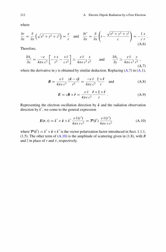
From the Maxwell’s equations, the electric and magnetic fields,
E D cB � Or and B D r � A ; (A.1)
of the radiation generated by any current density J are described from the potentialvector
A.r; t/ D 1
4�� c2
ZJ.r 0; t 0/jr � r 0j dV 0 ' 1
4�� c2 r
ZJ.r 0; t 0/dV 0 : (A.2)
The simplification jr�r 0j ' r is valid for point sources, or very far away, in relationto the radiation observation point r D rOr at the time instant t D t 0 C r=c. In the caseof a single electron oscillating with speed v at the origin, the above integral reducesto
ZJ.r 0; t 0/dV 0 D �ev.t 0/ : (A.3)
When Oz is set as the electron oscillation direction, i.e. v D vOz,
Ax.r; t/ D 0; Ay.r; t/ D 0; Az.r; t/ D �ev.t 0/4�� c2 r
and
B D r � A D Ox@Az
@y� Oy@Az
@x: (A.4)
The partial derivatives are obtained as follows:
@Az
@xD �e
4�� c2
�v
@
@x
�1
r
�C 1
r
@v
@x
�D �e
4�� c2
�� v
r2
@r
@xC 1
r
@v
@t 0@t 0
@x
�(A.5)
© Springer International Publishing Switzerland 2016S.L. Morelhão, Computer Simulation Tools for X-ray Analysis,Graduate Texts in Physics, DOI 10.1007/978-3-319-19554-4
211
212 A Electric Dipole Radiation by a Free Electron
where
@r
@xD @
@x
�px2 C y2 C z2
�D x
rand
@t 0
@xD @
@x
t �
px2 C y2 C z2
c
!D �1
c
x
r:
(A.6)Therefore,
@Az
@xD �e
4�� c2
��v x
r3� x Pv
c r2
�' e Pv
4�� c3
x
r2and
@Az
@y' e Pv
4�� c3
y
r2;
(A.7)where the derivative in y is obtained by similar deduction. Replacing (A.7) in (A.1),
B D e Pv4�� c3
yOx � xOyr2
D �e Pv4�� c3
Oz � Orr
and (A.8)
E D cB � Or D e Pv4�� c2
Or � Oz � Orr
: (A.9)
Representing the electron oscillation direction by O" and the radiation observationdirection by Os 0, we come to the general expression
E.r; t/ D Os 0 � O" � Os 0 e Pv.t 0/4�� r c2
D P.Os0/e Pv.t 0/
4�� r c2(A.10)
where P.Os0/ D Os 0 � O"� Os 0 is the vector polarization factor introduced in Sect. 1.1.1,(1.5). The other term of (A.10) is the amplitude of scattering given in (1.8), with Rand Rz in place of r and Pv, respectively.
Appendix BMatLab Routines
MatLab R�—The Language of Technical Computing, is the high-level language andinteractive environment used for developing most routines of this book. Simpleand compact, the language made it possible for more than 80 routines to be attachedhere. Other MatLab advantages are easy manipulation of matrixes and graphicalinterfaces, and the possibility of calling programs written in other languages suchas C, CCC, Java, and Fortran. An example of program in CCC is the routinesaxs.c that is available in the supporting information at the book’s website. Formore information on MatLab, go to http://www.mathworks.com/products/matlab/ .
Supporting Information for routines and worked exercises can befound at the book’s webpage http://xraybook.if.usp.br/ .
1. asfQ.mfunction f=asfQ(atom,x)%%%%%%%%%%%%%%%%%%%%%%%%%%%%%%%%%%%%%%%%%%%%%%%%%%%%%%%%%%%%%%%%%%%%%%%%%%%% Calculate atomic scattering factors, f0 %% Input: %% atom = element symbol, e.g. ’Ga’ %% x = sen(th)/lambda = 0.25*Q/pi (m-by-n array) (1/Angstrom) %% Output: %% f0(x) = c + sum_i ai * exp(-bi*x^2) i=1,2,3,4 %% in a m-by-n matrix format. %% Coefficients a1, a2, a3, a4, b1, b2, b3, b4, and c %% from file f0_CromerMann.dat available at http://xraybook.if.usp.br/ %%%%%%%%%%%%%%%%%%%%%%%%%%%%%%%%%%%%%%%%%%%%%%%%%%%%%%%%%%%%%%%%%%%%%%%%%%%%x = x.*x;sizeA = size(atom,2);mmax = cromermann(0);m = 1; CM=zeros(1,9); ctr = 1;
while ((ctr == 1) && (m < mmax + 1))line = cromermann(m);aux = find(line(1:8)==’ ’);n = aux(1);if (n==sizeA+1)X = line(1:n-1);if (X==atom)CM = sscanf(line(9:size(line,2)),’%f’)’;ctr = 0;
© Springer International Publishing Switzerland 2016S.L. Morelhão, Computer Simulation Tools for X-ray Analysis,Graduate Texts in Physics, DOI 10.1007/978-3-319-19554-4
213
214 B MatLab Routines
end;end;m = m + 1;
end;if (ctr==1) disp([’ Element ’ atom ’ not found!!!’]); return; end;f = CM(1)*exp(-CM(5)*x) + CM(2)*exp(-CM(6)*x) + CM(3)*exp(-CM(7)*x) + CM(4)*exp(-CM(8)*x) + CM(9);
function line=cromermann(nn)M = [’C 2.310000 1.020000 1.588600 0.865000 20.843900 10.207500 0.568700 51.651200 0.215600’;’Ga 15.235400 6.700600 4.359100 2.962300 3.066900 0.241200 10.780500 61.413500 1.718900’;’Ga3+ 12.692000 6.698830 6.066920 1.006600 2.812620 0.227890 6.364410 14.412200 1.535450’;’As 16.672300 6.070100 3.431300 4.277900 2.634500 0.264700 12.947900 47.797200 2.531000’];% Complete matrix of coefficients is available on the book’s webpageif (nn==0), line = size(M,1);else line = M(nn,:);end;
2. assintotic.mfunction M=assintotic(a,b,c,Qi,Qf,N,Na)%%%%%%%%%%%%%%%%%%%%%%%%%%%%%%%%%%%%%%%%%%%%%%%%%%%%%%%%%%%%%%%%%%%%%%%%%%%% Small-angle scattering of particles with rectangular dimensions %% Input: %% a,b,c = particles dimensions (Angstrom) %% Qi,Qf = Q-range, initial and final values (1/Angstrom) %% N = number of points in the scattering curve %% Na = number of random positions within particle’s volume a x b x c %% Ouptup M = [Q; I]’; N-by-2 array with the curve intensity x Q %% Usage: Z=assintotic(10,10,100,0.008,2.0,200,1000); %%%%%%%%%%%%%%%%%%%%%%%%%%%%%%%%%%%%%%%%%%%%%%%%%%%%%%%%%%%%%%%%%%%%%%%%%%%%N = fix(N);if (N>1), dQ = (Qf-Qi)/N; else disp(’ >>> Insufficient number of points!!!’); end;Q = Qi:dQ:Qf;Nq = size(Q,2);R = [a*rand(Na,1) b*rand(Na,1) c*rand(Na,1)];
I = zeros(1,Nq);for n=1:Na
for m = n+1:NaRnm = R(m,:)-R(n,:);QR = sqrt(Rnm*Rnm’)*Q;I = I + sin(QR)./QR;
end;end;M = [Q; I]’;
3. backadj.mfunction B=backadj(X,M)%%%%%%%%%%%%%%%%%%%%%%%%%%%%%%%%%%%%%%%%%%%%%%%%%%%%%%%%%%%%%%%%%%%%%%%%%%%% To adjust background noise of XRD pattern %% Input: %% X = x-axis (2theta or Q) values of the raw data %% M = ginput <-- MatLab command to get (x,y) coordinates by clicking %% on the figure window %% Output B = background noise in the raw data, estimated by linear %% interpolating the points obtained from the ginput command %%%%%%%%%%%%%%%%%%%%%%%%%%%%%%%%%%%%%%%%%%%%%%%%%%%%%%%%%%%%%%%%%%%%%%%%%%%%N=size(M,1);xa = M(1,1); ya = M(1,2);B=zeros(size(X));for n=2:Nxb = M(n,1); yb = M(n,2);Nx = X>xa & X<=xb;B(Nx) = (X(Nx)-xa)*((yb-ya)/(xb-xa)) + ya;
xa = xb; ya = yb;end;
4. benzeneonpsp.mfunction I=benzeneonpsp(thx,thy,thz,D,L,pixel,wl,prn)%%%%%%%%%%%%%%%%%%%%%%%%%%%%%%%%%%%%%%%%%%%%%%%%%%%%%%%%%%%%%%%%%%%%%%%%%%%% Intensity pattern of a molecule on cylindrical film (X-ray detector) %% Molecule: aromatic ring with 6 carbon atoms %% Input: %% thx, thy, and thz molecule rotation angles (deg) %% film radius D and length 2L, and size of pixel (mm) %% wl = wavelength (Angstrom) ou energy (eV) %% prn = 0 to suppress image preview %
B MatLab Routines 215
% Output: I = intensity on the pixel array %% Secondary routines required: asfQ.m %% Usage: %% >> I=benzeneonpsp(30,0,90,50,200,2,20000,1); %%%%%%%%%%%%%%%%%%%%%%%%%%%%%%%%%%%%%%%%%%%%%%%%%%%%%%%%%%%%%%%%%%%%%%%%%%%%rad = pi / 180;deg = 1/rad;if (wl < 1000) E = 12398.5 / wl; else E = wl; wl = 12398.5 / E; end;aux = 2 * pi / wl;s = [1 0 0];e = [0 0 1];dz = pixel;n = floor(2*L/dz);LimZ = 0.5*n*dz;
Z = -LimZ:dz:LimZ;Nz = size(Z,2);dphi = pixel / D;n = floor(pi/dphi);LimPhi = 0.5*(2*n-1)*dphi;phi = -LimPhi:dphi:LimPhi;Nphi = size(phi,2);D2 = D*D;
aux1 = D2*dz*dphi;Rn = i*benzene([thx thy thz]*rad);for nz = 1:Nzz = Z(nz);invr = 1/sqrt(z*z+D2);DOmega = aux1*invr*invr*invr;X(1:Nphi,nz)=z;
for np = 1:Nphiy = phi(np);cphi = cos(y);sphi = sin(y);sprime = invr*[D*cphi D*sphi z];p = cross(sprime,cross(e,sprime));p = p * p’;Q = aux * (sprime - s);modQ(np,nz) = norm(Q);F = sum(exp(Q*Rn));Ic(np,nz)= p*F*conj(F)*DOmega;Y(np,nz)= y*deg;
end;end;f = asfQ(’C’,(.25/pi)*modQ);I = real(f.*f.*Ic);if (prn~=0)
hf1=figure(1);clfset(hf1,’InvertHardcopy’, ’off’,’Color’,’w’)surf(X,Y,log10(I))axis imageshading interpset(gca,’FontSize’,14,’Color’,[0.93 0.93 0.93],’LineWidth’,1)set(gca,’YTick’,[-180 -120 -60 0 60 120 180],’ZTick’,[],’DataAspectRatio’,[1 1 0.3])colormap(jet)colorbar(’XColor’,’k’,’FontSize’,14,’Location’,’East’,’LineWidth’,1)xlabel(’film axis, z (mm)’,’FontSize’,18,’Rotation’,21)ylabel(’2\theta ({\circ})’,’FontSize’,18)
text(-1160,-2020,400,’Log(I)’,’FontSize’,14)end;
function Rn=benzene(Or)thx = Or(1); thy = Or(2); thz = Or(3);ra=1.4;th = [0 60 120 180 240 300] * (pi/180) + thx;r = ra*[zeros(1,6); cos(th); sin(th)];cthz = cos(thz);sthz = sin(thz);cthy = cos(thy);sthy = sin(thy);
Ry = [cthy 0 -sthy; 0 1 0; sthy 0 cthy];Rz = [cthz -sthz 0; sthz cthz 0; 0 0 1];Rn = Rz*Ry*r;
5. benzenesaxs1.mfunction M=benzenesaxs1(D,L,pixel,wl)%%%%%%%%%%%%%%%%%%%%%%%%%%%%%%%%%%%%%%%%%%%%%%%%%%%%%%%%%%%%%%%%%%%%%%%%%%%% Small angle X-ray scattering by %% a disperse system of benzene molecules %% Input: %% radius D (mm) and width 2L (mm) of the film (cylindric geometry) %% pixel = pixel size (mm) %% wl = wavelength (Angstrom) or energy (eV) %% Output M = [tth Ir Ic] %% | | | %% | | incoherent (Compton) intensity %
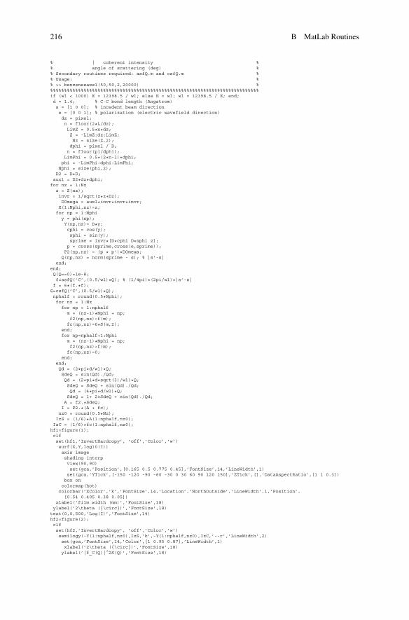
216 B MatLab Routines
% | coherent intensity %% angle of scattering (deg) %% Secondary routines required: asfQ.m and csfQ.m %% Usage: %% >> benzenesaxs1(50,50,2,20000) %%%%%%%%%%%%%%%%%%%%%%%%%%%%%%%%%%%%%%%%%%%%%%%%%%%%%%%%%%%%%%%%%%%%%%%%%%%%if (wl < 1000) E = 12398.5 / wl; else E = wl; wl = 12398.5 / E; end;d = 1.4; % C-C bond length (Angstrom)s = [1 0 0]; % incedent beam directione = [0 0 1]; % polarization (electric wavefield direction)dz = pixel;n = floor(2*L/dz);LimZ = 0.5*n*dz;Z = -LimZ:dz:LimZ;Nz = size(Z,2);dphi = pixel / D;n = floor(pi/dphi);LimPhi = 0.5*(2*n-1)*dphi;phi = -LimPhi:dphi:LimPhi;Nphi = size(phi,2);
D2 = D*D;aux1 = D2*dz*dphi;for nz = 1:Nzz = Z(nz);invr = 1/sqrt(z*z+D2);DOmega = aux1*invr*invr*invr;X(1:Nphi,nz)=z;
for np = 1:Nphiy = phi(np);Y(np,nz)= D*y;cphi = cos(y);sphi = sin(y);sprime = invr*[D*cphi D*sphi z];p = cross(sprime,cross(e,sprime));P2(np,nz) = (p * p’)*DOmega;Q(np,nz) = norm(sprime - s); % |s’-s|
end;end;Q(Q==0)=1e-8;f=asfQ(’C’,(0.5/wl)*Q); % (1/4pi)*(2pi/wl)*|s’-s|f = 6*(f.*f);S=csfQ(’C’,(0.5/wl)*Q);nphalf = round(0.5*Nphi);for nz = 1:Nz
for np = 1:nphalfm = (nz-1)*Nphi + np;f2(np,nz)=f(m);fc(np,nz)=6*S(m,2);
end;for np=nphalf+1:Nphim = (nz-1)*Nphi + np;f2(np,nz)=f(m);fc(np,nz)=0;
end;end;Qd = (2*pi*d/wl)*Q;SdeQ = sin(Qd)./Qd;Qd = (2*pi*d*sqrt(3)/wl)*Q;SdeQ = SdeQ + sin(Qd)./Qd;Qd = (4*pi*d/wl)*Q;SdeQ = 1+ 2*SdeQ + sin(Qd)./Qd;A = f2.*SdeQ;I = P2.*(A + fc);nz0 = round(0.5*Nz);
IzS = (1/6)*A(1:nphalf,nz0);IzC = (1/6)*fc(1:nphalf,nz0);hf1=figure(1);clfset(hf1,’InvertHardcopy’, ’off’,’Color’,’w’)surf(X,Y,log10(I))axis imageshading interpview(90,90)set(gca,’Position’,[0.165 0.5 0.775 0.45],’FontSize’,14,’LineWidth’,1)set(gca,’YTick’,[-150 -120 -90 -60 -30 0 30 60 90 120 150],’ZTick’,[],’DataAspectRatio’,[1 1 0.3])box oncolormap(hot)colorbar(’XColor’,’k’,’FontSize’,14,’Location’,’NorthOutside’,’LineWidth’,1,’Position’,[0.54 0.405 0.38 0.05])
xlabel(’film width (mm)’,’FontSize’,18)ylabel(’2\theta ({\circ})’,’FontSize’,18)text(0,0,500,’Log(I)’,’FontSize’,14)hf2=figure(2);clfset(hf2,’InvertHardcopy’, ’off’,’Color’,’w’)semilogy(-Y(1:nphalf,nz0),IzS,’k’,-Y(1:nphalf,nz0),IzC,’--r’,’LineWidth’,2)set(gca,’FontSize’,14,’Color’,[1 0.95 0.87],’LineWidth’,1)xlabel(’2\theta ({\circ})’,’FontSize’,18)ylabel(’|f_C(Q)|^2S(Q)’,’FontSize’,18)
B MatLab Routines 217
text(90,8,’Compton \downarrow’,’Color’,’r’,’FontSize’,18)axis tightgridM = [-Y(1:nphalf,nz0) IzS IzC];
6. benzenesaxs2.mfunction M=benzenesaxs2(wl)%%%%%%%%%%%%%%%%%%%%%%%%%%%%%%%%%%%%%%%%%%%%%%%%%%%%%%%%%%%%%%%%%%%%%%%%%%%% SAXS, structural function of the benzene molecule %% Input: %% wl = wavelength (Angstrom) or energy (eV) %% Output M = [Q; SofQ; SofQ1; SofQ2; SofQ3]’; %% | | | | | %% | | interference pattern of each atomic pair %% | structural function %% reciprocal vector module (1/Angstrom) %%%%%%%%%%%%%%%%%%%%%%%%%%%%%%%%%%%%%%%%%%%%%%%%%%%%%%%%%%%%%%%%%%%%%%%%%%%%if (wl < 1000) E = 12398.5 / wl; else E = wl; wl = 12398.5 / E; end;d = 1.4; % C-C bond length (Angstrom)Qmax = (4*pi/wl);dQ = Qmax/1000;Q = 0:dQ:Qmax;Q(1) = 1e-8;Qd1 = d*Q;Qd2 = (d*sqrt(3))*Q;Qd3 = (2*d)*Q;SofQ1 = sin(Qd1)./Qd1;
SofQ2 = sin(Qd2)./Qd2;SofQ3 = sin(Qd3)./Qd3;SofQ = 1+2*(SofQ1+SofQ2)+SofQ3;hf1=figure(1);clfset(hf1,’InvertHardcopy’, ’off’,’Color’,’w’)semilogy(Q,2+SofQ1,’--m’,Q,1.5+SofQ2,’--r’,Q,1+SofQ3,’--b’,’LineWidth’,1)legend(’ 140pm’,’ 243pm’,’ 280pm’)hold onsemilogy(Q,SofQ,’k’,’LineWidth’,1.5);hold offset(gca,’FontSize’,14,’Color’,[1 0.95 0.87],’LineWidth’,1,’YTick’,[0.7 0.8 0.9 1 1.5 2 2.5 3])xlabel(’Q (A^{-1})’,’FontSize’,18)ylabel(’S(Q)’,’FontSize’,18)
axis([0 Qmax 0.98*min(SofQ) 3.2])gridM = [Q; SofQ; SofQ1; SofQ2; SofQ3]’;
7. bragg.mfunction M=bragg(wl,A,H)%%%%%%%%%%%%%%%%%%%%%%%%%%%%%%%%%%%%%%%%%%%%%%%%%%%%%%%%%%%%%%%%%%%%%%%%%%%% Input: %% wl = wavelength (Angstrom) or energy (eV) %% A = [a b c alpha beta gamma], lattice parameters (Angstrom and deg) %% H = [h1 k1 l1; h2 k2 l2; ...], reflection indexes %% Output M = [ E wl 0 0; %% d thB 2thB Vc] %% | | | | %% | | | unit cell volume (Angstrom^3) %% | | 2theta Bragg (deg) %% | theta Bragg (deg) %% interplane distance (Angstrom) %% Usage: %% >> bragg(1.54,[],[]); %% >> bragg(8000,[4.9134 4.9134 5.4052 90 90 120],[1 0 0; 0 1 1]); %%%%%%%%%%%%%%%%%%%%%%%%%%%%%%%%%%%%%%%%%%%%%%%%%%%%%%%%%%%%%%%%%%%%%%%%%%%%rad = pi / 180;deg = 1/rad;if (wl < 1000) E = 12398.5 / wl; else E = wl; wl = 12398.5 / E; end;fprintf(’ Energy = %6.2feV (%8.6f A)\n’,E,wl);
if isempty(A) M = [E wl]; return; else M(1,:) = [E wl 0 0]; end;nm = size(A);if (nm(1)*nm(2)==1)A(1:3) = A(1)*ones(1,3);A(4:6) = [90 90 90];
elseif (nm(1)*nm(2)==2)A(1:3) = [A(1) A(1) A(2)];A(4:6) = [90 90 90];
end;A(4:6) = A(4:6)*rad;cosphi = cos(A(6)) - cos(A(5))*cos(A(4));cosphi = cosphi / (sin(A(5))*sin(A(4)));sinphi = sqrt(1-cosphi*cosphi);a1 = A(1) * [sin(A(5)) 0 cos(A(5))];
218 B MatLab Routines
a2 = A(2) * [sin(A(4))*cosphi sin(A(4))*sinphi cos(A(4))];a3 = A(3) * [0 0 1];a1r = cross(a2,a3);Vc = a1r*a1’;a1r = a1r/Vc;a2r = cross(a3,a1)/Vc;
a3r = cross(a1,a2)/Vc;Nr = size(H,1);for n=1:Nrq = H(n,1)*a1r + H(n,2)*a2r + H(n,3)*a3r;d = 1/sqrt(q*q’);sinth = 0.5*wl/d;
if (sinth > 1)fprintf(’ d(%d,%d,%d) = %7.5f A (reflection not allowed for this energy!!!)\n’,H(n,1),H(n,2),H(n,3),d);M(n+1,:) = [d 0 0 Vc];
elseth = asin(sinth)*deg;tth = 2*th;fprintf(’ d(%d,%d,%d) = %7.5f A, thB = %6.4f deg, 2thB = %6.4f deg\n’,H(n,1),H(n,2),H(n,3),d,th,tth);M(n+1,:) = [d th tth Vc];
end;end;
8. csfQ.mfunction S=csfQ(atom,X)%%%%%%%%%%%%%%%%%%%%%%%%%%%%%%%%%%%%%%%%%%%%%%%%%%%%%%%%%%%%%%%%%%%%%%%%%%%% Linear interpolation of tabulated values of the %% incoherent (Compton) scattering function, S(x,Z) %% Input: %% atom = element symbol from ’H’ to ’Cs’ (Z from 1 to 55) %% X = sin(th)/lambda = 0.25*Q/pi (1/Angstrom), e.g. X=0:0.05:2; %% Output S = [x f] %% | | %% | interpolated values of S(x,Z) %% sen(th)/lambda (1/Angstrom) %% %% Tabulated values S(x,Z) from file IncohScattFunction.txt available at %% http://xraybook.if.usp.br/ %%%%%%%%%%%%%%%%%%%%%%%%%%%%%%%%%%%%%%%%%%%%%%%%%%%%%%%%%%%%%%%%%%%%%%%%%%%%X(X<0)=0; X((X>2))=2;s=size(X); NofX=s(1)*s(2);sizeA = size(atom,2);W(1,:) = [.1 .2 .3 .4 .5 .6 .7 .8 .9 1.0 1.5 2.0];mmax = hubbell(0);m = 1; W(2,:)=zeros(1,12); ctr = 1;while ((ctr == 1) && (m < mmax+1))line = hubbell(m);aux = find(line(1:8)==’ ’);n = aux(1);if (n==sizeA+1)A = line(1:n-1);if (A==atom)W(2,:) = sscanf(line(9:size(line,2)),’%f’)’;ctr = 0;
end;end;m = m + 1;
end;if (ctr==1)
disp([’ Element ’ atom ’ not found!!! Using Cs instead...’]);W(2,:) = sscanf(line(9:size(line,2)),’%f’)’;
end;NofW = 12;for nx = 1:NofXx = X(nx);x2 = 0; f = 0;nw = 1;while (nw <= NofW)x1 = x2; y = f;x2 = W(1,nw); f = W(2,nw);if (x2 > x)f = (f - y) * (x - x1) / (x2 - x1) + y;nw = NofW;
end;nw = nw + 1;
end;S(nx,:) = [x f];
end;
function line=hubbell(m)M = [’C 1.039 2.604 3.643 4.184 4.478 4.690 4.878 5.051 5.208 5.348 5.781 5.930’;’N 1.080 2.858 4.097 4.792 5.182 5.437 5.635 5.809 5.968 6.113 6.630 6.860’;’O 0.977 2.799 4.293 5.257 5.828 6.175 6.411 6.596 6.755 6.901 7.462 7.764’;
B MatLab Routines 219
’Ca 3.105 5.690 7.981 9.790 11.157 12.163 12.953 13.635 14.256 14.830 16.921 17.970’];% Complete table of theoretical values is available on the book’s webpageif (m==0), line = size(M,1);else line = M(m,:);end;
9. debye.mfunction debye(ct,Qf,rab,sg)%%%%%%%%%%%%%%%%%%%%%%%%%%%%%%%%%%%%%%%%%%%%%%%%%%%%%%%%%%%%%%%%%%%%%%%%%%%% Comparison of numerical solutions of F = FT{G(u-rab)} %% with usual approximations %% Input: %% ct = 1 for F = G(u-rab).sin(Qu)/Qu, 2 for F = G(u-rab).sin(Qu), and %% 3 for F = G(u-rab).cos(Qu) %% Qf = upper limit of Q-range (1/Angstrom) %% rab = a value of interatomic distance (Angstrom) %% sg = Gaussian standard deviation (Angstroms), %% G(u-rab) = exp[-(u-rab)^2/2sg^2] %%%%%%%%%%%%%%%%%%%%%%%%%%%%%%%%%%%%%%%%%%%%%%%%%%%%%%%%%%%%%%%%%%%%%%%%%%%%if (sg < 0.005)disp(’ >>>> Standard deviation too small, use sg > 0.005 A!!!’)return;
end;if (rab >= 50)
disp(’ >>>> Interatomic distance too large, use rab < 50 A!!!’)return;
end;Nu = 10000;Umax = 200;du = Umax/Nu;U = 0:du:Umax;U(1) = 1e-8;Nq = 500;dq = Qf/Nq;Q = 0:dq:Qf;Q(1)=1e-8;
Nq = size(Q,2);G = (du/(sg*sqrt(2*pi)))*exp((-0.5/sg^2)*(U-rab).^2);Y = zeros(1,Nq);if (ct==1)
for n = 1:NqQu = Q(n)*U;Y(n) = sum(G.*sin(Qu)./Qu);
end;Qrab = rab*Q;dqm = sg/sqrt(2);Y2 = exp(-(dqm^2*(Q.*Q))).*(sin(Qrab)./Qrab);
ytext = ’FT\{G(u-rab)/4\piu^2\}’;elseif (ct==2)
for n = 1:NqQu = Q(n)*U;Y(n) = sum(G.*sin(Qu));
end;Qrab = rab*Q;dqm = sg/sqrt(2);Y2 = exp(-(dqm^2*(Q.*Q))).*sin(Qrab);
ytext = ’imag[FT\{G(u-rab)\}]’;else
for n = 1:NqQu = Q(n)*U;Y(n) = sum(G.*cos(Qu));
end;Qrab = rab*Q;dqm = sg/sqrt(2);Y2 = exp(-(dqm^2*(Q.*Q))).*cos(Qrab);
ytext = ’real[FT\{G(u-rab)\}]’;end;hf1=figure(1); clf; set(hf1,’InvertHardcopy’, ’off’,’Color’,’w’);plot(Q,Y,’r’,Q,Y2,’-.b’,’LineWidth’,2)axis tightset(gca,’FontSize’,14,’Color’,[0.93 0.93 0.93],’LineWidth’,1)
xlabel(’Q (A^{-1})’,’FontSize’,18)ylabel(ytext,’FontSize’,18)legend(’ numerical solution’,’ DW approximation’)
220 B MatLab Routines
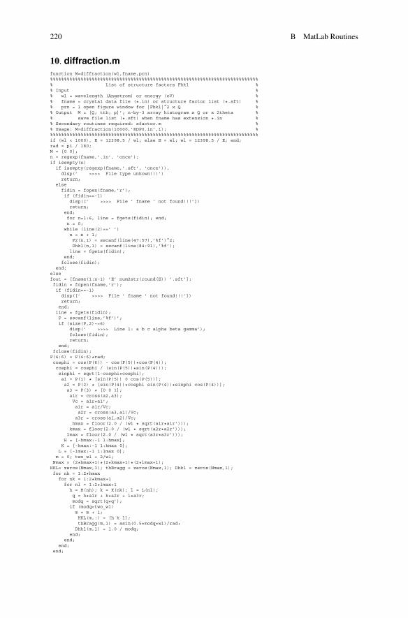
10. diffraction.mfunction M=diffraction(wl,fname,prn)%%%%%%%%%%%%%%%%%%%%%%%%%%%%%%%%%%%%%%%%%%%%%%%%%%%%%%%%%%%%%%%%%%%%%%%%%%%% List of structure factors Fhkl %% Input %% wl = wavelength (Angstrom) or energy (eV) %% fname = crystal data file (*.in) or structure factor list (*.sft) %% prn = 1 open figure window for |Fhkl|^2 x Q %% Output M = [Q; tth; p]’; n-by-3 array histogram x Q or x 2theta %% save file list (*.sft) when fname has extension *.in %% Secondary routines required: sfactor.m %% Usage: M=diffraction(10000,’KDP0.in’,1); %%%%%%%%%%%%%%%%%%%%%%%%%%%%%%%%%%%%%%%%%%%%%%%%%%%%%%%%%%%%%%%%%%%%%%%%%%%%if (wl < 1000), E = 12398.5 / wl; else E = wl; wl = 12398.5 / E; end;rad = pi / 180;M = [0 0];n = regexp(fname,’.in’, ’once’);if isempty(n)if isempty(regexp(fname,’.sft’, ’once’)),
disp(’ >>>> File type unkown!!!’)return;
elsefidin = fopen(fname,’r’);if (fidin==-1)disp([’ >>>> File ’ fname ’ not found!!!’])return;
end;for n=1:6, line = fgets(fidin); end;n = 0;while (line(2)==’ ’)n = n + 1;F2(n,1) = sscanf(line(47:57),’%f’)^2;Dhkl(n,1) = sscanf(line(84:91),’%f’);line = fgets(fidin);
end;fclose(fidin);
end;elsefout = [fname(1:n-1) ’E’ num2str(round(E)) ’.sft’];fidin = fopen(fname,’r’);if (fidin==-1)
disp([’ >>>> File ’ fname ’ not found!!!’])return;end;
line = fgets(fidin);P = sscanf(line,’%f’)’;if (size(P,2)~=6)
disp(’ >>>> Line 1: a b c alpha beta gamma’);fclose(fidin);return;
end;fclose(fidin);P(4:6) = P(4:6)*rad;cosphi = cos(P(6)) - cos(P(5))*cos(P(4));cosphi = cosphi / (sin(P(5))*sin(P(4)));sinphi = sqrt(1-cosphi*cosphi);a1 = P(1) * [sin(P(5)) 0 cos(P(5))];a2 = P(2) * [sin(P(4))*cosphi sin(P(4))*sinphi cos(P(4))];a3 = P(3) * [0 0 1];a1r = cross(a2,a3);Vc = a1r*a1’;a1r = a1r/Vc;a2r = cross(a3,a1)/Vc;a3r = cross(a1,a2)/Vc;hmax = floor(2.0 / (wl * sqrt(a1r*a1r’)));kmax = floor(2.0 / (wl * sqrt(a2r*a2r’)));lmax = floor(2.0 / (wl * sqrt(a3r*a3r’)));H = [-hmax:-1 1:hmax];K = [-kmax:-1 1:kmax 0];L = [-lmax:-1 1:lmax 0];
m = 0; two_wl = 2/wl;Nmax = (2*hmax+1)*(2*kmax+1)*(2*lmax+1);
HKL= zeros(Nmax,3); thBragg = zeros(Nmax,1); Dhkl = zeros(Nmax,1);for nh = 1:2*hmax
for nk = 1:2*kmax+1for nl = 1:2*lmax+1h = H(nh); k = K(nk); l = L(nl);q = h*a1r + k*a2r + l*a3r;modq = sqrt(q*q’);if (modq<two_wl)m = m + 1;HKL(m,:) = [h k l];thBragg(m,1) = asin(0.5*modq*wl)/rad;Dhkl(m,1) = 1.0 / modq;
end;end;
end;end;
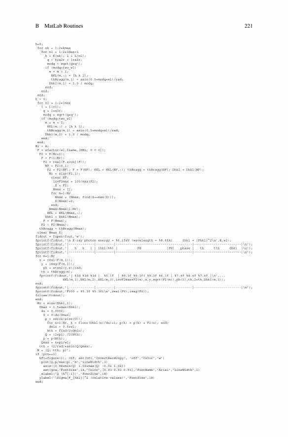
B MatLab Routines 221
h=0;for nk = 1:2*kmax
for nl = 1:2*lmax+1k = K(nk); l = L(nl);q = k*a2r + l*a3r;modq = sqrt(q*q’);if (modq<two_wl)m = m + 1;HKL(m,:) = [h k l];thBragg(m,1) = asin(0.5*modq*wl)/rad;Dhkl(m,1) = 1.0 / modq;
end;end;
end;k = 0;for nl = 1:2*lmax
l = L(nl);q = l*a3r;modq = sqrt(q*q’);if (modq<two_wl)m = m + 1;HKL(m,:) = [h k l];thBragg(m,1) = asin(0.5*modq*wl)/rad;Dhkl(m,1) = 1.0 / modq;
end;end;Nr = m;F = sfactor(wl,fname,[HKL; 0 0 0]);F0 = F(Nr+1);F = F(1:Nr);F2 = real(F.*conj(F));NF = F2>0.1;F2 = F2(NF); F = F(NF); HKL = HKL(NF,:); thBragg = thBragg(NF); Dhkl = Dhkl(NF);Nr = size(F2,1);clear NF;invF2max = 100/max(F2);X = F2;Nmax = [];for m=1:NrNmax = [Nmax; find(X==max(X))];X(Nmax)=0;
end;Nmax=Nmax(1:Nr);HKL = HKL(Nmax,:);Dhkl = Dhkl(Nmax);F = F(Nmax);F2 = F2(Nmax);
thBragg = thBragg(Nmax);clear Nmax X;fidout = fopen(fout,’w’);fprintf(fidout,’\n X-ray photon energy = %6.1feV (wavelength = %8.6fA) Ihkl = |Fhkl|^2\n’,E,wl);fprintf(fidout,’|-------------|---------|---------------------------------------|------------------------|\n’);fprintf(fidout,’| h k l | Ihkl(%%) | FH |FH| phase | th tth dhkl |\n’);fprintf(fidout,’|-------------|---------|---------------------------------------|------------------------|\n’);for m=1:Nrx = real(F(m,1));y = imag(F(m,1));ph = atan2(y,x)/rad;th = thBragg(m);
fprintf(fidout,’| %3d %3d %3d | %5.1f | %9.3f %9.3fi %9.3f %6.1f | %7.4f %8.4f %7.4f |\n’,...HKL(m,1),HKL(m,2),HKL(m,3),invF2max*F2(m),x,y,sqrt(F2(m)),ph(1),th,2*th,Dhkl(m,1));
end;fprintf(fidout,’|-------------|---------|---------------------------------------|------------------------|\n’);fprintf(fidout,’F000 = %5.3f %5.3fi\n’,real(F0),imag(F0));fclose(fidout);end;Nr = size(Dhkl,1);Umax = 1.5*max(Dhkl);du = 0.0002;U = 0:du:Umax;p = zeros(size(U));for n=1:Nr, k = floor(Dhkl(n)/du)+1; p(k) = p(k) + F2(n); end;dmin = 0.5*wl;Nth = find(U>dmin);Q = (2*pi)./U(Nth);p = p(Nth);Qmax = 4*pi/wl;
tth = (2/rad)*asin(Q/Qmax);M = [Q; tth; p]’;if (prn==1)hf1=figure(1); clf; set(hf1,’InvertHardcopy’, ’off’,’Color’,’w’)plot(Q,p/max(p),’b’,’LineWidth’,3)axis([0.98*min(Q) 1.02*max(Q) -0.02 1.02])set(gca,’FontSize’,14,’Color’,[0.93 0.93 0.93],’FontName’,’Arial’,’LineWidth’,1)xlabel(’Q (A^{-1})’,’FontSize’,18)
ylabel(’\Sigma|F_{hkl}|^2 (relative values)’,’FontSize’,18)end;
222 B MatLab Routines
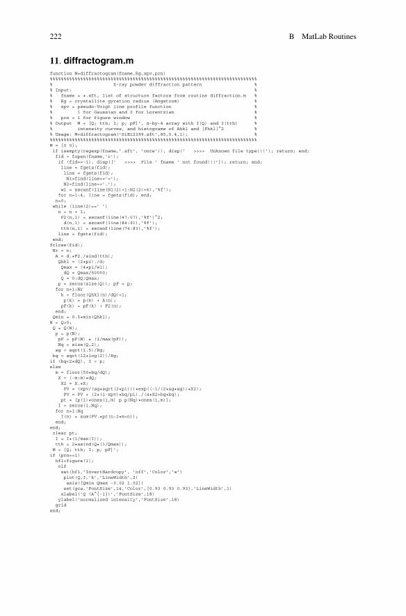
11. diffractogram.mfunction M=diffractogram(fname,Rg,xpv,prn)%%%%%%%%%%%%%%%%%%%%%%%%%%%%%%%%%%%%%%%%%%%%%%%%%%%%%%%%%%%%%%%%%%%%%%%%%%%% X-ray powder diffraction pattern %% Input: %% fname = *.sft, list of structure factors from routine diffraction.m %% Rg = crystallite gyration radius (Angstrom) %% xpv = pseudo-Voigt line profile function %% 1 for Gaussian and 0 for Lorentzian %% prn = 1 for figure window %% Output M = [Q; tth; I; p; pF]’, n-by-4 array with I(Q) and I(tth) %% intensity curves, and histograms of Ahkl and |Fhkl|^2 %% Usage: M=diffractogram(’SiE12399.sft’,85,0.4,1); %%%%%%%%%%%%%%%%%%%%%%%%%%%%%%%%%%%%%%%%%%%%%%%%%%%%%%%%%%%%%%%%%%%%%%%%%%%%M = [0 0];if isempty(regexp(fname,’.sft’, ’once’)), disp(’ >>>> Unknown file type!!!’); return; end;fid = fopen(fname,’r’);if (fid==-1), disp([’ >>>> File ’ fname ’ not found!!!’]); return; end;line = fgets(fid);line = fgets(fid);N1=find(line==’=’);N2=find(line==’.’);wl = sscanf(line(N1(2)+1:N2(2)+6),’%f’);for n=1:4, line = fgets(fid); end;
n=0;while (line(2)==’ ’)
n = n + 1;F2(n,1) = sscanf(line(47:57),’%f’)^2;d(n,1) = sscanf(line(84:91),’%f’);tth(n,1) = sscanf(line(74:83),’%f’);line = fgets(fid);
end;fclose(fid);Nr = n;A = d.*F2./sind(tth);Qhkl = (2*pi)./d;Qmax = (4*pi/wl);dQ = Qmax/50000;Q = 0:dQ:Qmax;p = zeros(size(Q)); pF = p;
for n=1:Nrk = floor(Qhkl(n)/dQ)+1;p(k) = p(k) + A(n);pF(k) = pF(k) + F2(n);
end;Qmin = 0.5*min(Qhkl);N = Q>0;Q = Q(N);p = p(N);pF = pF(N) * (1/max(pF));Nq = size(Q,2);
sg = sqrt(1.5)/Rg;bq = sqrt(12*log(2))/Rg;if (bq<2*dQ), I = p;elsem = floor(50*bq/dQ);X = (-m:m)*dQ;X2 = X.*X;PV = (xpv/(sg*sqrt(2*pi)))*exp((-1/(2*sg*sg))*X2);PV = PV + (2*(1-xpv)*bq/pi)./(4*X2+bq*bq);
pt = [p(1)*ones(1,m) p p(Nq)*ones(1,m)];I = zeros(1,Nq);
for n=1:NqI(n) = sum(PV.*pt(n:2*m+n));
end;end;clear pt;I = I*(1/max(I));tth = 2*asind(Q*(1/Qmax));M = [Q; tth; I; p; pF]’;if (prn==1)hf1=figure(1);clfset(hf1,’InvertHardcopy’, ’off’,’Color’,’w’)plot(Q,I,’k’,’LineWidth’,2)axis([Qmin Qmax -0.02 1.02])set(gca,’FontSize’,14,’Color’,[0.93 0.93 0.93],’LineWidth’,1)xlabel(’Q (A^{-1})’,’FontSize’,18)ylabel(’normalized intensity’,’FontSize’,18)
gridend;
B MatLab Routines 223
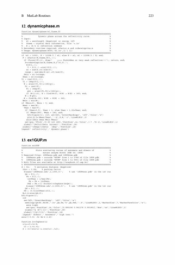
12. dynamicphase.mfunction dynamicphase(wl,fname,H)%%%%%%%%%%%%%%%%%%%%%%%%%%%%%%%%%%%%%%%%%%%%%%%%%%%%%%%%%%%%%%%%%%%%%%%%%%%% Dynamic phase across the reflectivity curve %% Input: %% wl = wavelength (Angstrom) or energy (eV) %% fname = crystal data information, file ’*.in’ %% H = [h k l] reflection indexes %% Secondary routines required: sfactor.m and rcdarwinprins.m %% Usage: dynamicphase(8000,’Si.in’,[1 1 1]) %%%%%%%%%%%%%%%%%%%%%%%%%%%%%%%%%%%%%%%%%%%%%%%%%%%%%%%%%%%%%%%%%%%%%%%%%%%%if (wl < 1000), E = 12398.5 / wl; else E = wl; wl = 12398.5 / E; end;F = sfactor(E,fname,H(1,:));if (F*conj(F)<1), disp(’ >>>> Forbidden or very weak reflection!!!’); return; end;S=rcdarwinprins(E,fname,H,2^30,0).’;X=S(1,:);Y = S(2,:).*conj(S(2,:));xc = sum(X.*Y)/sum(Y);range = sum(abs(X-xc).*Y)/sum(Y);
Xmin = xc-3*range;Xmax = xc+3*range;Yr = real(S(2,:));Yi = imag(S(2,:));W = atan2(Yi,Yr)*(180/pi);Fr = real(F);Fi = imag(F);phi = atan2(Fi,Fr)*(180/pi);if (W(1)<0), N = find(W<0); W(N) = W(N) + 360; end;W = W-phi;
N = find(W<-90); W(N) = W(N) + 360;Wmin = min(W);if (Wmin>0), Wmin = 0; end;Wmax = max(W);Ymax = max(Y);if (Ymax>0.5), Ymax = 1; else Ymax = 1.02*Ymax; end;if (Wmax<180), Wmax = 180; end;hf1=figure(1); clf; set(hf1,’InvertHardcopy’, ’off’,’Color’,’w’)plot(X,Y*(Wmax/Ymax),’--k’,X,W,’-r’,’LineWidth’,2)axis([Xmin Xmax Wmin Wmax])set(gca,’YTick’,[0 60 120 180],’FontSize’,14,’Color’,[.7 .78 1],’LineWidth’,1)
xlabel(’\Delta\theta (arcsec)’,’FontSize’,18)ylabel(’\Omega(\theta) (deg)’,’FontSize’,18)legend(’ reflectivity’,’ dynamic phase’)
13. ex1GUP.mfunction ex1GUP%%%%%%%%%%%%%%%%%%%%%%%%%%%%%%%%%%%%%%%%%%%%%%%%%%%%%%%%%%%%%%%%%%%%%%%%%%%% Plots scattering curves of monomers and dimers of %% mutant enzyme H166G (PDB ID: 1GUP) %% Required files: 1GUPmono.pdb and 1GUPdime.pdb %% 1GUPmono.pdb = records "ATOM" from 1 to 2784 of file 1GUP.pdb %% 1GUPdime.pdb = records "ATOM" from 1 to 5551 of file 1GUP.pdb %% Both files are available at http://xraybook.if.usp.br/ %% %%%%%%%%%%%%%%%%%%%%%%%%%%%%%%%%%%%%%%%%%%%%%%%%%%%%%%%%%%%%%%%%%%%%%%%%%d = 54; % exclusion distance (Angstrom)rhov = 0.08; % packing factorS=saxs(’1GUPmono.ndu’,2,1000,0)’; % use ’1GUPmono.pdb’ in the 1st runQm = S(1,:);Pm = S(2,:);invPmax = 1/max(Pm);Pm = Pm * invPmax;PmS = Pm.*(1-(8*rhov)*tfsphere(d*Qm));
S=saxs(’1GUPdime.ndu’,2,1000,0)’; % use ’1GUPdime.pdb’ in the 1st runQd = S(1,:);
Pd = (0.5*invPmax)*S(2,:);N=1:4:size(Qd,2);hf1=figure(1);clfset(hf1,’InvertHardcopy’, ’off’,’Color’,’w’)semilogy(Qd(N),Pd(N),’-ro’,Qm,Pm,’k’,Qm,PmS,’-.k’,’LineWidth’,2,’MarkerSize’,7,’MarkerFaceColor’,’w’);axis tightset(gca,’FontSize’,14,’Color’,[0.890196 0.941176 0.901961],’Box’,’on’,’LineWidth’,1)xlabel(’Q (A^{-1})’,’FontSize’,18)
ylabel(’I(Q)/I(0)’,’FontSize’,18)legend(’ dimers’,’ monomers’,’ high conc.’)axis([-0.01 .52 8e-4 2.4])
function Z=tfsphere(u)u(u<=0)=1e-8;u3 = u.*u.*u;Z = 3*((sin(u)-u.*cos(u))./u3);
224 B MatLab Routines
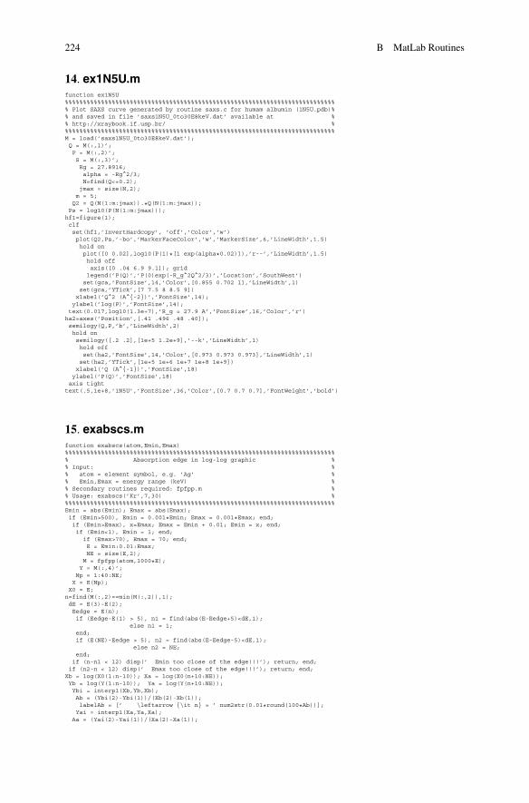
14. ex1N5U.mfunction ex1N5U%%%%%%%%%%%%%%%%%%%%%%%%%%%%%%%%%%%%%%%%%%%%%%%%%%%%%%%%%%%%%%%%%%%%%%%%%%%% Plot SAXS curve generated by routine saxs.c for humam albumin (1N5U.pdb)%% and saved in file ’saxs1N5U_0to30E8keV.dat’ available at %% http://xraybook.if.usp.br/ %%%%%%%%%%%%%%%%%%%%%%%%%%%%%%%%%%%%%%%%%%%%%%%%%%%%%%%%%%%%%%%%%%%%%%%%%%%%M = load(’saxs1N5U_0to30E8keV.dat’);Q = M(:,1)’;P = M(:,2)’;S = M(:,3)’;Rg = 27.8916;alpha = -Rg^2/3;N=find(Q<=0.2);jmax = size(N,2);m = 5;
Q2 = Q(N(1:m:jmax)).*Q(N(1:m:jmax));Ps = log10(P(N(1:m:jmax)));hf1=figure(1);clfset(hf1,’InvertHardcopy’, ’off’,’Color’,’w’)plot(Q2,Ps,’-bo’,’MarkerFaceColor’,’w’,’MarkerSize’,6,’LineWidth’,1.5)hold onplot([0 0.02],log10(P(1)*[1 exp(alpha*0.02)]),’r--’,’LineWidth’,1.5)hold offaxis([0 .04 6.9 9.1]); gridlegend(’P(Q)’,’P(0)exp(-R_g^2Q^2/3)’,’Location’,’SouthWest’)set(gca,’FontSize’,14,’Color’,[0.855 0.702 1],’LineWidth’,1)set(gca,’YTick’,[7 7.5 8 8.5 9])xlabel(’Q^2 (A^{-2})’,’FontSize’,14);
ylabel(’log(P)’,’FontSize’,14);text(0.017,log10(1.3e+7),’R_g = 27.9 A’,’FontSize’,16,’Color’,’r’)ha2=axes(’Position’,[.41 .496 .48 .40]);semilogy(Q,P,’b’,’LineWidth’,2)hold onsemilogy([.2 .2],[1e+5 1.2e+9],’--k’,’LineWidth’,1)hold offset(ha2,’FontSize’,14,’Color’,[0.973 0.973 0.973],’LineWidth’,1)set(ha2,’YTick’,[1e+5 1e+6 1e+7 1e+8 1e+9])xlabel(’Q (A^{-1})’,’FontSize’,18)
ylabel(’P(Q)’,’FontSize’,18)axis tighttext(.5,1e+8,’1N5U’,’FontSize’,36,’Color’,[0.7 0.7 0.7],’FontWeight’,’bold’)
15. exabscs.mfunction exabscs(atom,Emin,Emax)%%%%%%%%%%%%%%%%%%%%%%%%%%%%%%%%%%%%%%%%%%%%%%%%%%%%%%%%%%%%%%%%%%%%%%%%%%%% Absorption edge in log-log graphic %% Input: %% atom = element symbol, e.g. ’Ag’ %% Emin,Emax = energy range (keV) %% Secondary routines required: fpfpp.m %% Usage: exabscs(’Kr’,7,30) %%%%%%%%%%%%%%%%%%%%%%%%%%%%%%%%%%%%%%%%%%%%%%%%%%%%%%%%%%%%%%%%%%%%%%%%%%%%Emin = abs(Emin); Emax = abs(Emax);if (Emin>500), Emin = 0.001*Emin; Emax = 0.001*Emax; end;if (Emin>Emax), x=Emax; Emax = Emin + 0.01; Emin = x; end;if (Emin<1), Emin = 1; end;if (Emax>70), Emax = 70; end;E = Emin:0.01:Emax;NE = size(E,2);M = fpfpp(atom,1000*E);Y = M(:,4)’;Np = 1:40:NE;
X = E(Np);X0 = E;n=find(M(:,2)==min(M(:,2)),1);dE = E(3)-E(2);Eedge = E(n);if (Eedge-E(1) > 5), n1 = find(abs(E-Eedge+5)<dE,1);
else n1 = 1;end;if (E(NE)-Eedge > 5), n2 = find(abs(E-Eedge-5)<dE,1);
else n2 = NE;end;
if (n-n1 < 12) disp(’ Emin too close of the edge!!!’); return; end;if (n2-n < 12) disp(’ Emax too close of the edge!!!’); return; end;Xb = log(X0(1:n-10)); Xa = log(X0(n+10:NE));Yb = log(Y(1:n-10)); Ya = log(Y(n+10:NE));Ybi = interp1(Xb,Yb,Xb);Ab = (Ybi(2)-Ybi(1))/(Xb(2)-Xb(1));labelAb = [’ \leftarrow {\it n} = ’ num2str(0.01*round(100*Ab))];Yai = interp1(Xa,Ya,Xa);
Aa = (Yai(2)-Yai(1))/(Xa(2)-Xa(1));
B MatLab Routines 225
labelAa = [’ \leftarrow {\it n} = ’ num2str(0.01*round(100*Aa))];hf1=figure(1);clfset(hf1,’InvertHardcopy’, ’off’,’Color’,’w’)loglog(exp(Xb),exp(Ybi),’b’,exp(Xa),exp(Yai),’r’,’LineWidth’,2)hold onloglog(exp([max(Xb) min(Xa)]),exp([min(Ybi) max(Yai)]),’k’,’LineWidth’,2)loglog(X,Y(Np),’ko’,’MarkerFaceColor’,’w’,’MarkerSize’,6,’LineWidth’,1)hold offset(gca,’FontSize’,14,’Color’,[0.93 0.93 0.93],’LineWidth’,1)
ylabel(’\sigma_a (barn)’,’FontSize’,18)xlabel(’Energy (keV)’,’FontSize’,18)axis tight; gridnb = round(0.2*(1+n-10));na = round(0.3*(n+10+NE));text(X0(nb),Y(nb),labelAb,’FontSize’,18,’Color’,’b’)text(X0(na),Y(na),labelAa,’FontSize’,18,’Color’,’r’)fprintf(’\n Edge = %0.3f keV\n’,Eedge)Bbi = Y(n-10)/X0(n-10)^(Ab);
fprintf(’ below edge: %0.5gE^{%0.5f}\n’,Bbi,Ab);Bai = Y(n+10)/X0(n+10)^(Aa);fprintf(’ above edge: %0.5gE^{%0.5f}\n\n’,Bai,Aa);
16. exanomalousignal.mfunction exanomalousignal%%%%%%%%%%%%%%%%%%%%%%%%%%%%%%%%%%%%%%%%%%%%%%%%%%%%%%%%%%%%%%%%%%%%%%%%%%%% Reflectivity curves below and above the Ga K-edge (@ 10360eV) %% Secondary routines required: rcdarwinsprins.m %% Required files: GaAs.in %%%%%%%%%%%%%%%%%%%%%%%%%%%%%%%%%%%%%%%%%%%%%%%%%%%%%%%%%%%%%%%%%%%%%%%%%%%%S=rcdarwinprins(10300,’GaAs.in’,[1 1 7],4096,0).’;X1=S(1,:);N = find(X1>-180 & X1<180);X1=X1(N);Y1=S(2,N).*conj(S(2,N));Y1b=S(3,N).*conj(S(3,N));S=rcdarwinprins(10400,’GaAs.in’,[1 1 7],4096,0).’;X2=S(1,:);
N = find(X2>-180 & X2<180);X2=X2(N);Y2=S(2,N).*conj(S(2,N));Y2b=S(3,N).*conj(S(3,N));c1 = [.87 .92 .98]; c2 = [.86 .86 .86]; c3 = [.85 .16 0];hf1=figure(1); clf; set(hf1,’InvertHardcopy’, ’off’,’Color’,’w’)area(X1-180,Y1,’EdgeColor’,’k’,’FaceColor’,’w’,’LineWidth’,2)hold onarea(X1-180,Y1b,’EdgeColor’,c3,’FaceColor’,c2,’LineWidth’,2)area(X2+180,Y2,’EdgeColor’,’k’,’FaceColor’,’w’,’LineWidth’,2)area(X2+180,Y2b,’EdgeColor’,c3,’FaceColor’,c2,’LineWidth’,2)hold offaxis([-360 400 0 3e-3])set(gca,’FontName’,’Arial’,’FontSize’,14,’Color’,c1,’LineWidth’,1)xlabel(’\Delta\theta’,’FontSize’,18)
ylabel(’reflectivity, |R_N(\theta)|^2’,’FontSize’,18)legend(’ ( 1, 1, 7)’,’ (-1,-1,-7)’)S=rcdarwinprins(10300,’GaAs.in’,[1 1 7],2^30,0)’;X1=S(1,:);N = find(X1>-1 & X1<8);X1=X1(N);Y1=S(2,N).*conj(S(2,N));Y1b=S(3,N).*conj(S(3,N));S=rcdarwinprins(10400,’GaAs.in’,[1 1 7],2^30,0)’;X2=S(1,:);
N = find(X2>-1 & X2<8);X2=X2(N);Y2=S(2,N).*conj(S(2,N));Y2b=S(3,N).*conj(S(3,N));hf2=figure(2); clf; set(hf2,’InvertHardcopy’, ’off’,’Color’,’w’)area(X1-3,Y1,’EdgeColor’,’k’,’FaceColor’,’w’,’LineWidth’,2)hold onarea(X1-3,Y1b,’EdgeColor’,c3,’FaceColor’,c2,’LineWidth’,2)area(X2+3,Y2,’EdgeColor’,’k’,’FaceColor’,’w’,’LineWidth’,2)area(X2+3,Y2b,’EdgeColor’,c3,’FaceColor’,c2,’LineWidth’,2)hold offaxis([-4 11 0 1])set(gca,’FontName’,’Arial’,’FontSize’,14,’Color’,c1,’LineWidth’,1)
xlabel(’\Delta\theta’,’FontSize’,18)ylabel(’reflectivity, |R(\theta)|^2’,’FontSize’,18)legend(’ ( 1, 1, 7)’,’ (-1,-1,-7)’)
226 B MatLab Routines
17. exasf.mfunction exasf%%%%%%%%%%%%%%%%%%%%%%%%%%%%%%%%%%%%%%%%%%%%%%%%%%%%%%%%%%%%%%%%%%%%%%%%%%%% Atomic scattering factors for atoms and ions %% with X-rays of two different energies %% %% Secondary routines required: asfQ.m %%%%%%%%%%%%%%%%%%%%%%%%%%%%%%%%%%%%%%%%%%%%%%%%%%%%%%%%%%%%%%%%%%%%%%%%%%%%S1=asftth(20000,’Ga’);S2=asftth(20000,’Ga3+’);S3=asftth(8000,’Ga’);S4=asftth(8000,’Ga3+’);n=size(S1,1);hf1=figure(1);clfset(hf1,’InvertHardcopy’, ’off’,’Color’,’w’)
plot(S1(:,1),S1(:,2),’b’,’LineWidth’,1)set(gca,’FontSize’,14,’Color’,[0.93 0.93 0.93],’LineWidth’,1)hold onplot(S2(:,1),S2(:,2),’r’,’LineWidth’,1)plot(S3(:,1),S3(:,2),’bo’,’MarkerFaceColor’,’w’,’MarkerSize’,4,’LineWidth’,1)plot(S4(:,1),S4(:,2),’r^’,’MarkerFaceColor’,’w’,’MarkerSize’,4,’LineWidth’,1)hold offxlabel(’Q (A^{-1})’,’FontSize’,18)ylabel(’atomic scattering factor, f(Q)’,’FontSize’,18)axis([0 21 5 32])legend(’Ga (20kev)’,’Ga^{3+} (20kev)’,’Ga (8kev)’,’Ga^{3+} (8kev)’)hf1=figure(2);clfset(hf1,’InvertHardcopy’, ’off’,’Color’,’w’)
plot(S2(:,3),S2(:,4),’--r’,S2(:,3),-S2(:,4),’--r’,’LineWidth’,2)set(gca,’FontSize’,14,’Color’,[0.93 0.93 0.93],’LineWidth’,1)hold onplot(S1(:,3),S1(:,4),’b’,S1(:,3),-S1(:,4),’b’,’LineWidth’,2)plot(S4(:,3),S4(:,4),’--r’,S4(:,3),-S4(:,4),’--r’,’LineWidth’,2)plot(S3(:,3),S3(:,4),’b’,S3(:,3),-S3(:,4),’b’,’LineWidth’,2)plot([-1 1],[0 0],’k’,[0 0],[1 -1],’k’,’LineWidth’,1)hold offxlabel(’x’,’FontSize’,18)ylabel(’y’,’FontSize’,18)xmin=min([S1(n,3) S2(n,3) S3(n,3) S4(n,3)]);xmax=max([S1(1,2) S2(1,2) S3(1,2) S4(1,2)]);ymax=max(max([S1(:,4) S2(:,4) S3(:,4) S4(:,4)]));
ymin=-ymax;axis(1.12*[xmin xmax ymin ymax])text(-10,8,’ \leftarrow 8keV’,’FontSize’,18,’Color’,’k’)text(-4.5,-3,’ \leftarrow 20keV’,’FontSize’,18,’Color’,’k’)text(30.5,4,’\downarrow’,’FontSize’,18,’Color’,’b’)text(30,7,’Ga’,’FontSize’,18,’Color’,’b’)text(20,0.5,’ Ga^{3+} \rightarrow’,’FontSize’,18,’Color’,’r’)grid
function S=asftth(wl,atom)if (wl > 100) wl = 12398.5 / wl; end;dx = 0.01;x = [0:dx:1];tth = 2*asin(x);x = (1/wl)*x;f = asfQ(atom,x);S(:,1) = (4*pi)*x;
S(:,2) = f;S(:,3) = f .* cos(tth);S(:,4) = f.* sin(tth);
18. excompton.mfunction M=excompton(wl)%%%%%%%%%%%%%%%%%%%%%%%%%%%%%%%%%%%%%%%%%%%%%%%%%%%%%%%%%%%%%%%%%%%%%%%%%%%% Coherent and incoherent (Compton) intensities scattered by %% one electron with different probability density functions: %% I) |psi(r)|^2 constant within a sphere of radius a=0.5A %% II) |psi(r)|^2 of the hydrogen 1s orbital %% wl = wavelength (Angstrom) or energy (eV) %%%%%%%%%%%%%%%%%%%%%%%%%%%%%%%%%%%%%%%%%%%%%%%%%%%%%%%%%%%%%%%%%%%%%%%%%%%%if (wl < 100) E = 12398.5 / wl; else E = wl; wl = 12398.5 / E; end;a = 0.53; % Bohr radius (Angstrom)tth = (0:0.005:1)*pi;tth(1)=1e-6;x = cos(tth);P2 = 0.5*(1+x.*x);
Qa = (4*pi*a/wl)*sin(0.5*tth);tth = tth * (180/pi);x2 = Qa.*Qa;x = 3*(sin(Qa)-Qa.*cos(Qa))./(x2.*Qa);fI2 = x.*x;
B MatLab Routines 227
Icoer1 = P2.*fI2;Icomp1 = P2.*(1-fI2);x = 1+0.25*x2;x = 1./(x.*x);fII2 = x.*x;
Icoer2 = P2.*fII2;Icomp2 = P2.*(1-fII2);hf1=figure(1);clfset(hf1,’InvertHardcopy’, ’off’,’Color’,’w’)plot(tth,Icoer1,’b’,tth,Icoer2,’r’,’LineWidth’,2)hold onplot(tth,Icomp1,’b--’,tth,Icomp2,’r--’,tth,Icoer1+Icomp1,’k-.’,’LineWidth’,1.5)hold offset(gca,’FontSize’,14,’Color’,[0.854902 0.701961 1],’LineWidth’,1,’YTick’,[0 0.2 0.4 0.6 0.8 1.0])ylabel(’I(Q) / \Phi r_e^2 d\Omega’,’FontSize’,18)xlabel(’2\theta (\circ)’,’FontSize’,18)
axis tighttext(40,0.8,’ \leftarrow I_{Th}’,’FontSize’,18,’Color’,’k’)M = [tth; Icoer1; Icomp1; Icoer2; Icomp2]’;X=(0:0.01:4)*a;XX = X.*X;Y1 = (3/a^3)*XX(X<=a);
n = size(Y1,2)+1;Y1(n) = 0;Y2 = (4/a^3)*(XX.*exp(-(2/a)*X));ha2=axes(’Position’,[.70 .25 .19 .37]);plot(X(1:n),Y1,’b’,X,Y2,’r’,’LineWidth’,2)set(ha2,’FontSize’,14,’Color’,[0.9 0.9 1])ylabel(’4\pir^2|\psi(r)|^2 (A^{-1})’,’FontSize’,14)xlabel(’r (A)’,’FontSize’,14)
axis tighttext(0.5,4,’ \leftarrow I’,’FontSize’,18,’Color’,’b’,’FontName’,’Times’)text(0.8,1,’ \leftarrow II’,’FontSize’,18,’Color’,’r’,’FontName’,’Times’)
19. excritangle.mfunction excritangle%%%%%%%%%%%%%%%%%%%%%%%%%%%%%%%%%%%%%%%%%%%%%%%%%%%%%%%%%%%%%%%%%%%%%%%%%%%% Critical angle for total external reflection in %% gold and glass (amorphous alpha-quartz) surfaces %% Secondary routines required: fpfpp.m %%%%%%%%%%%%%%%%%%%%%%%%%%%%%%%%%%%%%%%%%%%%%%%%%%%%%%%%%%%%%%%%%%%%%%%%%%%%E = 4:0.1:20; % energy range (keV)deg = 180/pi;wl = 12.3985./E;rewl2_pi = (2.818e-5*wl.*wl/pi);f = fpfpp(’Si’,E);fpSi = f(:,2)’;f = fpfpp(’O’,E);fpO = f(:,2)’;f = fpfpp(’Au’,E);fpAu = f(:,2)’;Yglass = (1/113)*rewl2_pi .* (52 + 2*fpSi + 3*fpO);Yglass = sqrt(Yglass)*deg;Yglass0 = (52/113)*rewl2_pi;Yglass0 = sqrt(Yglass0)*deg;Ygold = (1/67.8)*rewl2_pi .* (316 + 4*fpAu);Ygold = sqrt(Ygold)*deg;Ygold0 = (316/67.8)*rewl2_pi;Ygold0 = sqrt(Ygold0)*deg;hf = figure; clf; set(hf,’InvertHardcopy’, ’off’,’Color’,’w’)plot(E,Yglass,’b’,E,Yglass0,’--b’,E,Ygold,’r’,E,Ygold0,’--r’,’LineWidth’,2)set(gca,’FontSize’,14,’LineWidth’,1);axis tight;
xlabel(’Energy (keV)’,’FontSize’,18)ylabel(’\theta_c (deg)’,’FontSize’,18)legend(’ glass surface’,’ glass surf. no res.’,’ gold surface’,’ gold surf. no res.’)
20. excsf.mfunction excsf(atom,E1,E2,p)%%%%%%%%%%%%%%%%%%%%%%%%%%%%%%%%%%%%%%%%%%%%%%%%%%%%%%%%%%%%%%%%%%%%%%%%%%%% Coherent and incoherent scattering by an atom %% comparison for two different energies %% Input: %% atom = element symbol, e.g. ’C’ %% E1,E2 = two energy values (keV) %% p = 0, 1, and 2 for sigma-, pi-, and non-polarized X-rays %% Secondary routines required: asfQ.m and csfQ.m %
228 B MatLab Routines
% Usage: %% >> excsf(’C’,8,20,0); %%%%%%%%%%%%%%%%%%%%%%%%%%%%%%%%%%%%%%%%%%%%%%%%%%%%%%%%%%%%%%%%%%%%%%%%%%%%if (E1>500) E1 = 0.001*abs(E1); end;if (E2>500) E2 = 0.001*abs(E2); end;labelE1 = [num2str(round(E1)) ’keV’];labelE2 = [num2str(round(E2)) ’keV’];tth = (0:1:360)*(pi/180);if (p==1)P2 = cos(tth)’;P2 = P2.*P2;labelP = ’\pi polarization’;
elseif (p==2)P2 = cos(tth)’;P2 = 0.5*(1+P2.*P2);labelP = ’unpolarized’;
elseP2 = ones(size(tth,2),1);labelP = ’\sigma polarization’;
end;S1=asfxQ(E1,atom,tth,P2);S2=csfxQ(E1,atom,tth,P2);
S3=asfxQ(E2,atom,tth,P2);S4=csfxQ(E2,atom,tth,P2);xmax = S1(1,2); xmin = min(S4(:,3)); ymax = max(S1(:,4)); ymin =-ymax;hf1=figure(1);clfset(hf1,’InvertHardcopy’, ’off’,’Color’,’w’)plot(S1(:,3),S1(:,4),’b’,’LineWidth’,2)set(gca,’FontSize’,14,’Color’,[0.93 0.93 0.93],’LineWidth’,1,’Position’,[0.13 0.02 0.775 0.9])hold onplot(S2(:,3),S2(:,4),’--b’,’LineWidth’,1)plot(S3(:,3),S3(:,4),’r’,’LineWidth’,2)plot(S4(:,3),S4(:,4),’--r’,’LineWidth’,1)plot([-1 1],[0 0],’k’,[0 0],[1 -1],’k’,’LineWidth’,1)hold offxlabel(’x’,’FontSize’,18)ylabel(’y’,’FontSize’,18)axis imageaxis([1.2*xmin 1.05*xmax 1.1*ymin 1.1*ymax])
text(0,0,atom,’FontSize’,36,’Color’,[0.855 0.702 1],’FontWeight’,’bold’)gridlegend([’ coherent ’ labelE1],[’ compton ’ labelE1],[’ coherent ’ labelE2],[’ compton ’ labelE2])title([atom ’, ’ labelP],’FontSize’,18)
function S=asfxQ(wl,atom,tth,P2)wl = 12.3985 / wl;x = sin(0.5*tth)/wl;S(:,1) = (4*pi) * x;F = asfQ(atom,x)’;F2(:,1) = F.*F.*P2;
S(:,2) = F2;S(:,3) = F2 .* cos(tth’);S(:,4) = F2 .* sin(tth’);
function S=csfxQ(wl,atom,tth,P2)wl = 12.3985 / wl;x = sin(0.5*tth)/wl;S(:,1) = (4*pi) * x;Y = csfQ(atom,x);F = Y(:,2).*P2;
S(:,2) = F;S(:,3) = F .* cos(tth’);S(:,4) = F .* sin(tth’);
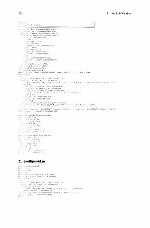
21. exellipsoid.mfunction exellipsoidX=0:0.01:1;Nx = size(X,1);w2 = X.*X;Rg2 = sqrt(0.2*(2*w2 + 1)); % oplateRg1 = sqrt(0.2*(2 + w2)); % prolatehf1=figure(1);clfset(hf1,’InvertHardcopy’, ’off’,’Color’,’w’)plot(X,Rg1,’b’,X,Rg2,’r’,’LineWidth’,2)axis([0 1 0.4 0.8])set(gca,’FontSize’,14,’Color’,[0.93 0.93 0.93],’LineWidth’,1)legend(’ oblate’,’ prolate’,4)
xlabel(’ratio of the dimensions, {\it w}’,’FontSize’,18);ylabel(’R_g / L’,’FontSize’,18);grid
B MatLab Routines 229
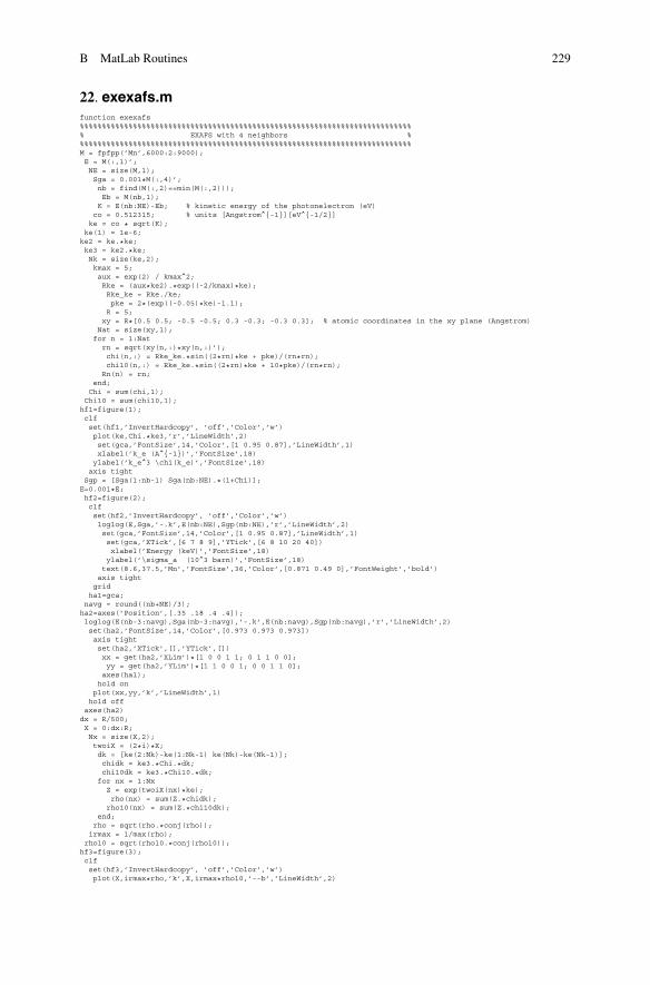
22. exexafs.mfunction exexafs%%%%%%%%%%%%%%%%%%%%%%%%%%%%%%%%%%%%%%%%%%%%%%%%%%%%%%%%%%%%%%%%%%%%%%%%%%%% EXAFS with 4 neighbors %%%%%%%%%%%%%%%%%%%%%%%%%%%%%%%%%%%%%%%%%%%%%%%%%%%%%%%%%%%%%%%%%%%%%%%%%%%%M = fpfpp(’Mn’,6000:2:9000);E = M(:,1)’;NE = size(M,1);Sga = 0.001*M(:,4)’;nb = find(M(:,2)==min(M(:,2)));Eb = M(nb,1);K = E(nb:NE)-Eb; % kinetic energy of the photonelectron (eV)co = 0.512315; % units [Angstrom^{-1}][eV^{-1/2}]
ke = co * sqrt(K);ke(1) = 1e-6;ke2 = ke.*ke;ke3 = ke2.*ke;Nk = size(ke,2);kmax = 5;aux = exp(2) / kmax^2;Rke = (aux*ke2).*exp((-2/kmax)*ke);Rke_ke = Rke./ke;pke = 2*(exp((-0.05)*ke)-1.1);R = 5;xy = R*[0.5 0.5; -0.5 -0.5; 0.3 -0.3; -0.3 0.3]; % atomic coordinates in the xy plane (Angstrom)Nat = size(xy,1);for n = 1:Natrn = sqrt(xy(n,:)*xy(n,:)’);chi(n,:) = Rke_ke.*sin((2*rn)*ke + pke)/(rn*rn);chi10(n,:) = Rke_ke.*sin((2*rn)*ke + 10*pke)/(rn*rn);
Rn(n) = rn;end;
Chi = sum(chi,1);Chi10 = sum(chi10,1);hf1=figure(1);clfset(hf1,’InvertHardcopy’, ’off’,’Color’,’w’)plot(ke,Chi.*ke3,’r’,’LineWidth’,2)set(gca,’FontSize’,14,’Color’,[1 0.95 0.87],’LineWidth’,1)xlabel(’k_e (A^{-1})’,’FontSize’,18)ylabel(’k_e^3 \chi(k_e)’,’FontSize’,18)
axis tightSgp = [Sga(1:nb-1) Sga(nb:NE).*(1+Chi)];E=0.001*E;hf2=figure(2);clfset(hf2,’InvertHardcopy’, ’off’,’Color’,’w’)loglog(E,Sga,’-.k’,E(nb:NE),Sgp(nb:NE),’r’,’LineWidth’,2)set(gca,’FontSize’,14,’Color’,[1 0.95 0.87],’LineWidth’,1)set(gca,’XTick’,[6 7 8 9],’YTick’,[6 8 10 20 40])xlabel(’Energy (keV)’,’FontSize’,18)ylabel(’\sigma_a (10^3 barn)’,’FontSize’,18)text(8.6,37.5,’Mn’,’FontSize’,36,’Color’,[0.871 0.49 0],’FontWeight’,’bold’)axis tightgrid
ha1=gca;navg = round((nb+NE)/3);ha2=axes(’Position’,[.35 .18 .4 .4]);loglog(E(nb-3:navg),Sga(nb-3:navg),’-.k’,E(nb:navg),Sgp(nb:navg),’r’,’LineWidth’,2)set(ha2,’FontSize’,14,’Color’,[0.973 0.973 0.973])axis tightset(ha2,’XTick’,[],’YTick’,[])xx = get(ha2,’XLim’)*[1 0 0 1 1; 0 1 1 0 0];yy = get(ha2,’YLim’)*[1 1 0 0 1; 0 0 1 1 0];axes(ha1);hold onplot(xx,yy,’k’,’LineWidth’,1)
hold offaxes(ha2)dx = R/500;X = 0:dx:R;Nx = size(X,2);twoiX = (2*i)*X;dk = [ke(2:Nk)-ke(1:Nk-1) ke(Nk)-ke(Nk-1)];chidk = ke3.*Chi.*dk;chi10dk = ke3.*Chi10.*dk;
for nx = 1:NxZ = exp(twoiX(nx)*ke);rho(nx) = sum(Z.*chidk);rho10(nx) = sum(Z.*chi10dk);
end;rho = sqrt(rho.*conj(rho));
irmax = 1/max(rho);rho10 = sqrt(rho10.*conj(rho10));hf3=figure(3);clfset(hf3,’InvertHardcopy’, ’off’,’Color’,’w’)plot(X,irmax*rho,’k’,X,irmax*rho10,’--b’,’LineWidth’,2)
230 B MatLab Routines
set(gca,’FontSize’,14,’Color’,[.961 .922 .922],’LineWidth’,1,’YTickLabel’,[])xlabel(’interatomic distance, u (A)’,’FontSize’,18)ylabel(’F(u) (arb. units.)’,’FontSize’,18)axis tightgridlegend(’ small variation, \delta_n ’,’ huge variation, 10\delta_n’)hold on
for n=1:Natplot([Rn(n) Rn(n)],[0 1],’r’,’LineWidth’,1)
end;hold offhf4=figure(4);clfset(hf4,’InvertHardcopy’, ’off’,’Color’,’w’)ha4a=axes(’Position’,[0.1 0.2 0.38 0.6]);set(ha4a,’FontSize’,14,’Color’,[.961 .922 .922],’LineWidth’,1);plot(ke,pke,’r’,’LineWidth’,2)
xlabel(’k_e (A^{-1})’,’FontSize’,18)ylabel(’\delta_n (radians)’,’FontSize’,18)axis tight; gridha4b=axes(’Position’,[0.6 0.2 0.38 0.6]);set(ha4b,’FontSize’,14,’Color’,[.961 .922 .922],’LineWidth’,1);plot(ke,Rke,’r’,’LineWidth’,2)set(ha4b,’YTick’,[0 .2 .4 .6 .8])xlabel(’k_e (A^{-1})’,’FontSize’,18)
ylabel(’R_n (A)’,’FontSize’,18)axis tightgrid
23. exexafsmap.mfunction exexafsmap%%%%%%%%%%%%%%%%%%%%%%%%%%%%%%%%%%%%%%%%%%%%%%%%%%%%%%%%%%%%%%%%%%%%%%%%%%%% EXAFS with 4 neighbors %%%%%%%%%%%%%%%%%%%%%%%%%%%%%%%%%%%%%%%%%%%%%%%%%%%%%%%%%%%%%%%%%%%%%%%%%%%%E = 200; % eVR = 5; % Angstromrad = pi / 180;k = 0.512315*sqrt(E);dr = R / 100;M = -R:dr:R;Np = size(M,2);xy = [0 0; 0.5 0.5; -0.5 -0.5; 0.3 -0.3; -0.3 0.3] * R;for n = 1:5 modR(n) = sqrt(xy(n,:)*xy(n,:)’); end;psh = k * modR;
an = 0.1; kan = k * an;A = [1 i i i i]./[1 modR(2:5)];for n = 1:Npy = M(n);for m = 1:Np
x = M(m);for nn = 1:5ra2 = [x y] - xy(nn,:);ra = sqrt(ra2*ra2’);if (ra<an) ra = an; end;kr = k * ra;arg = kr + psh(nn);den = kan / kr;psi(nn) = A(nn) * exp(i*arg) * den;
end;z = sum(psi);Z(n,m) = z*conj(z);X(n,m) = x; Y(n,m) = y;
end;end;logZ = log10(Z);hf1=figure(1);clfset(hf1,’InvertHardcopy’, ’off’,’Color’,’w’)surf(X,Y,logZ)axis tightshading interpset(gca,’FontSize’,14,’Color’,[0.93 0.93 0.93],’LineWidth’,1)set(gca,’ZTick’,[],’DataAspectRatio’,[.15 .15 1])colormap(jet)view(150,30)xlabel(’x (A)’,’FontSize’,18,’Rotation’,18)
ylabel(’y (A)’,’FontSize’,18,’Rotation’,-45 )colorbar(’XColor’,’k’,’FontSize’,14,’Location’,’East’,’LineWidth’,1)text(0,0,1,’log(P)’,’FontSize’,18,’Rotation’,90)
B MatLab Routines 231
24. exfpfpp.mfunction Z=exfpfpp(atom,Emin,Emax)%%%%%%%%%%%%%%%%%%%%%%%%%%%%%%%%%%%%%%%%%%%%%%%%%%%%%%%%%%%%%%%%%%%%%%%%%%%% Coherent scattering cross-section (Rayleigh) with atomic resonance %% Input: %% atom = element symbol, e.g. ’Se’ %% Emin,Emax = energy range from Emin to Emax (keV) %% Output Z = [E f’ f" sga sgR sgRr] %% | | | | | | %% | | | | | cross-section with resonance (barn) %% | | | | cross-section without resonance (barn) %% | | | absorption cross-section (barn) %% | | imaginary term (in electron number) %% | real term (in electron number) %% energy (eV) %% Secondary routines required: asfQ.m and fpfpp.m %% Usage: %% >> Z=exfpfpp(’Se’,3,23); %%%%%%%%%%%%%%%%%%%%%%%%%%%%%%%%%%%%%%%%%%%%%%%%%%%%%%%%%%%%%%%%%%%%%%%%%%%%Emin = abs(Emin); Emax = abs(Emax);if (Emax < Emin) E = Emax; Emax = Emin; Emin = E; end;if (Emin>500) Emin = 0.001*Emin; Emax = 0.001*Emax; end;if (Emin<1) Emin = 1; end;if (Emax>70) Emax = 70; end;if (Emax-Emin<0.020) E = [Emin Emin+0.01]; dE = 0.01;
else E = Emin:0.01:Emax; dE = E(3)-E(2);end;
NE = size(E,2);M = fpfpp(atom,1000*E);rad = pi/180;re = 2.818e-15; % (m)hc = 12.3985; % (keV.A)invWL = E/hc;dtth = 0.2; % (deg)TTH = 0:dtth:180; % (deg)X = TTH * rad;dx = dtth * rad;aux1 = pi * re * re * dx * 1e+28;
SinG = sin(X);PSinG = (2-SinG.*SinG).*SinG;for nn = 1:NEfres = M(nn,2:3);f = asfQ(atom,invWL(nn)*sin(0.5*X));fr = f + fres(1) +i*fres(2);f = f.*f;fr = fr.*conj(fr);I(nn) = aux1*sum(PSinG.*f);
Ir(nn) = aux1*sum(PSinG.*fr);end;Z = M;c = size(Z,2);Z(:,c+1:c+2) = [I; Ir]’;hf1=figure(1);clfset(hf1,’InvertHardcopy’, ’off’,’Color’,’w’)plot(E,I,’k--’,E,Ir,’k’,’LineWidth’,2)set(gca,’FontSize’,14,’Color’,[0.854902 0.701961 1],’LineWidth’,1)ylabel(’\sigma_R (barn)’,’FontSize’,18)xlabel(’Energy (keV)’,’FontSize’,18)axis tight
legend(’ without res.’,’ with res.’,3)n=find(M(:,2)==min(M(:,2)));if isempty(n)n1 = 1; n2 = NE; n = (n1+n2)/2;
elseEedge = E(n);if (Eedge-E(1) > 5)
n1 = find(abs(E-Eedge+5)<dE);else n1 = 1;end;if (E(NE)-Eedge > 5)
n2 = find(abs(E-Eedge-5)<dE);else n2 = NE;
end;endn1 = n1(1); n2 = n2(1);ha2=axes(’Position’,[.48 .45 .4 .4]);plot(E(n1:n2),M(n1:n2,2),’b’,E(n1:n2),M(n1:n2,3),’r’,’LineWidth’,2)set(ha2,’FontSize’,14,’Color’,[0.93 0.93 0.93])ylabel(’resonant amplitude’,’FontSize’,14)
xlabel(’Energy (keV)’,’FontSize’,14)axis tightlegend(’f \prime’,’f \prime\prime’,4)
232 B MatLab Routines
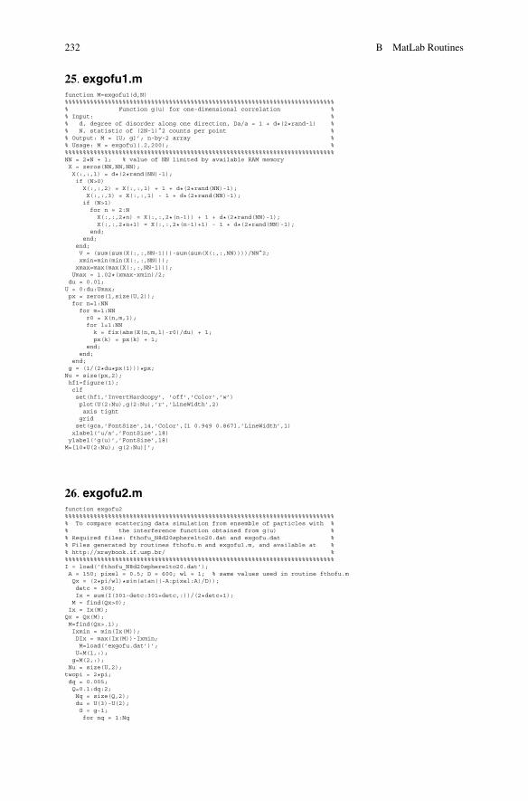
25. exgofu1.mfunction M=exgofu1(d,N)%%%%%%%%%%%%%%%%%%%%%%%%%%%%%%%%%%%%%%%%%%%%%%%%%%%%%%%%%%%%%%%%%%%%%%%%%%%% Function g(u) for one-dimensional correlation %% Input: %% d, degree of disorder along one direction, Da/a = 1 + d*(2*rand-1) %% N, statistic of (2N-1)^2 counts per point %% Output: M = [U; g]’; n-by-2 array %% Usage: M = exgofu1(.2,200); %%%%%%%%%%%%%%%%%%%%%%%%%%%%%%%%%%%%%%%%%%%%%%%%%%%%%%%%%%%%%%%%%%%%%%%%%%%%NN = 2*N + 1; % value of NN limited by available RAM memoryX = zeros(NN,NN,NN);X(:,:,1) = d*(2*rand(NN)-1);if (N>0)X(:,:,2) = X(:,:,1) + 1 + d*(2*rand(NN)-1);X(:,:,3) = X(:,:,1) - 1 + d*(2*rand(NN)-1);if (N>1)for n = 2:NX(:,:,2*n) = X(:,:,2*(n-1)) + 1 + d*(2*rand(NN)-1);X(:,:,2*n+1) = X(:,:,2*(n-1)+1) - 1 + d*(2*rand(NN)-1);
end;end;
end;V = (sum(sum(X(:,:,NN-1)))-sum(sum(X(:,:,NN))))/NN^2;xmin=min(min(X(:,:,NN)));xmax=max(max(X(:,:,NN-1)));
Umax = 1.02*(xmax-xmin)/2;du = 0.01;U = 0:du:Umax;px = zeros(1,size(U,2));for n=1:NN
for m=1:NNr0 = X(n,m,1);for l=1:NNk = fix(abs(X(n,m,l)-r0)/du) + 1;px(k) = px(k) + 1;
end;end;
end;g = (1/(2*du*px(1)))*px;Nu = size(px,2);hf1=figure(1);clfset(hf1,’InvertHardcopy’, ’off’,’Color’,’w’)plot(U(2:Nu),g(2:Nu),’r’,’LineWidth’,2)axis tightgridset(gca,’FontSize’,14,’Color’,[1 0.949 0.867],’LineWidth’,1)
xlabel(’u/a’,’FontSize’,18)ylabel(’g(u)’,’FontSize’,18)M=[10*U(2:Nu); g(2:Nu)]’;
26. exgofu2.mfunction exgofu2%%%%%%%%%%%%%%%%%%%%%%%%%%%%%%%%%%%%%%%%%%%%%%%%%%%%%%%%%%%%%%%%%%%%%%%%%%%% To compare scattering data simulation from ensemble of particles with %% the interference function obtained from g(u) %% Required files: fthofu_N8d20sphere1to20.dat and exgofu.dat %% Files generated by routines fthofu.m and exgofu1.m, and available at %% http://xraybook.if.usp.br/ %%%%%%%%%%%%%%%%%%%%%%%%%%%%%%%%%%%%%%%%%%%%%%%%%%%%%%%%%%%%%%%%%%%%%%%%%%%%I = load(’fthofu_N8d20sphere1to20.dat’);A = 150; pixel = 0.5; D = 600; wl = 1; % same values used in routine fthofu.mQx = (2*pi/wl)*sin(atan((-A:pixel:A)/D));detc = 300;Ix = sum(I(301-detc:301+detc,:))/(2*detc+1);
M = find(Qx>0);Ix = Ix(M);Qx = Qx(M);M=find(Qx>.1);Ixmin = min(Ix(M));DIx = max(Ix(M))-Ixmin;M=load(’exgofu.dat’)’;U=M(1,:);
g=M(2,:);Nu = size(U,2);twopi = 2*pi;dq = 0.005;Q=0.1:dq:2;Nq = size(Q,2);du = U(3)-U(2);G = g-1;for nq = 1:Nq
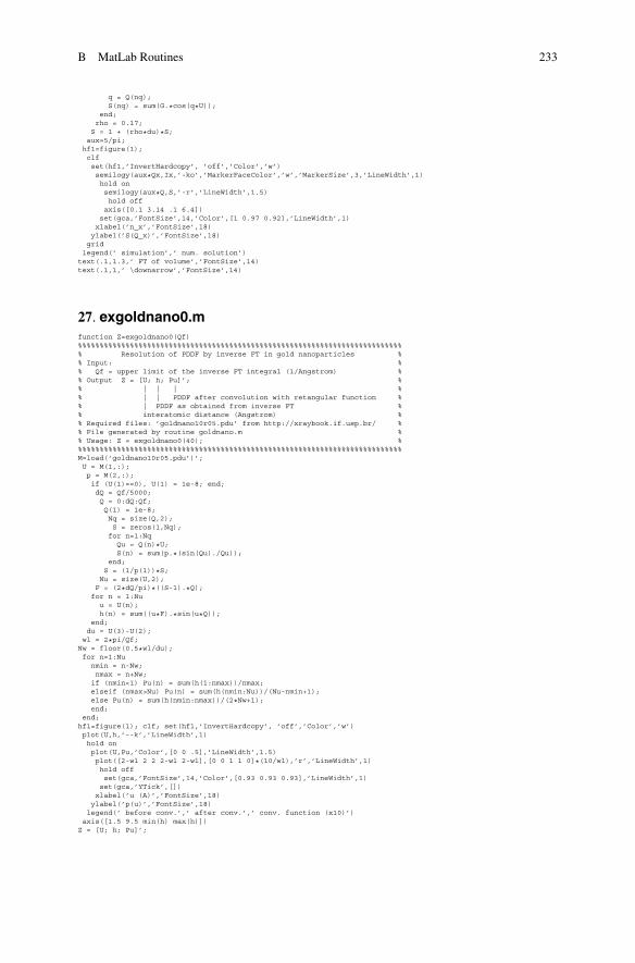
B MatLab Routines 233
q = Q(nq);S(nq) = sum(G.*cos(q*U));
end;rho = 0.17;S = 1 + (rho*du)*S;
aux=5/pi;hf1=figure(1);clfset(hf1,’InvertHardcopy’, ’off’,’Color’,’w’)semilogy(aux*Qx,Ix,’-ko’,’MarkerFaceColor’,’w’,’MarkerSize’,3,’LineWidth’,1)hold onsemilogy(aux*Q,S,’-r’,’LineWidth’,1.5)hold offaxis([0.1 3.14 .1 6.4])set(gca,’FontSize’,14,’Color’,[1 0.97 0.92],’LineWidth’,1)xlabel(’n_x’,’FontSize’,18)ylabel(’S(Q_x)’,’FontSize’,18)
gridlegend(’ simulation’,’ num. solution’)text(.1,1.3,’ FT of volume’,’FontSize’,14)text(.1,1,’ \downarrow’,’FontSize’,14)
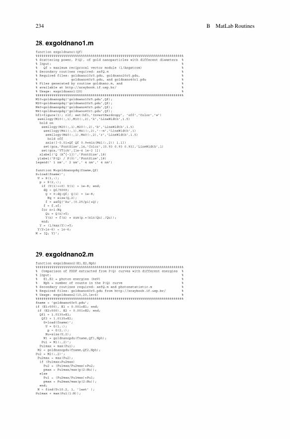
27. exgoldnano0.mfunction Z=exgoldnano0(Qf)%%%%%%%%%%%%%%%%%%%%%%%%%%%%%%%%%%%%%%%%%%%%%%%%%%%%%%%%%%%%%%%%%%%%%%%%%%%% Resolution of PDDF by inverse FT in gold nanoparticles %% Input: %% Qf = upper limit of the inverse FT integral (1/Angstrom) %% Output Z = [U; h; Pu]’; %% | | | %% | | PDDF after convolution with retangular function %% | PDDF as obtained from inverse FT %% interatomic distance (Angstrom) %% Required files: ’goldnano10r05.pdu’ from http://xraybook.if.usp.br/ %% File generated by routine goldnano.m %% Usage: Z = exgoldnano0(40); %%%%%%%%%%%%%%%%%%%%%%%%%%%%%%%%%%%%%%%%%%%%%%%%%%%%%%%%%%%%%%%%%%%%%%%%%%%%M=load(’goldnano10r05.pdu’)’;U = M(1,:);p = M(2,:);if (U(1)==0), U(1) = 1e-8; end;dQ = Qf/5000;Q = 0:dQ:Qf;Q(1) = 1e-8;Nq = size(Q,2);S = zeros(1,Nq);for n=1:NqQu = Q(n)*U;S(n) = sum(p.*(sin(Qu)./Qu));
end;S = (1/p(1))*S;Nu = size(U,2);F = (2*dQ/pi)*((S-1).*Q);
for n = 1:Nuu = U(n);h(n) = sum((u*F).*sin(u*Q));
end;du = U(3)-U(2);wl = 2*pi/Qf;Nw = floor(0.5*wl/du);for n=1:Nu
nmin = n-Nw;nmax = n+Nw;if (nmin<1) Pu(n) = sum(h(1:nmax))/nmax;elseif (nmax>Nu) Pu(n) = sum(h(nmin:Nu))/(Nu-nmin+1);else Pu(n) = sum(h(nmin:nmax))/(2*Nw+1);end;
end;hf1=figure(1); clf; set(hf1,’InvertHardcopy’, ’off’,’Color’,’w’)plot(U,h,’--k’,’LineWidth’,1)hold onplot(U,Pu,’Color’,[0 0 .5],’LineWidth’,1.5)plot([2-wl 2 2 2-wl 2-wl],[0 0 1 1 0]*(10/wl),’r’,’LineWidth’,1)hold offset(gca,’FontSize’,14,’Color’,[0.93 0.93 0.93],’LineWidth’,1)set(gca,’YTick’,[])xlabel(’u (A)’,’FontSize’,18)ylabel(’p(u)’,’FontSize’,18)
legend(’ before conv.’,’ after conv.’,’ conv. function (x10)’)axis([1.5 9.5 min(h) max(h)])Z = [U; h; Pu]’;
234 B MatLab Routines
28. exgoldnano1.mfunction exgoldnano1(Qf)%%%%%%%%%%%%%%%%%%%%%%%%%%%%%%%%%%%%%%%%%%%%%%%%%%%%%%%%%%%%%%%%%%%%%%%%%%%% Scattering power, P(Q), of gold nanoparticles with different diameters %% Input: %% Qf = maximum reciprocal vector module (1/Angstrom) %% Secondary routines required: asfQ.m %% Required files: goldnano10r5.pdu, goldnano20r5.pdu, %% goldnano40r5.pdu, and goldnano40r1.pdu %% Files generated by routine goldnano.m, and %% available at http://xraybook.if.usp.br/ %% Usage: exgoldnano1(20) %%%%%%%%%%%%%%%%%%%%%%%%%%%%%%%%%%%%%%%%%%%%%%%%%%%%%%%%%%%%%%%%%%%%%%%%%%%%M10=goldnanopdq(’goldnano10r5.pdu’,Qf);M20=goldnanopdq(’goldnano20r5.pdu’,Qf);M40=goldnanopdq(’goldnano40r5.pdu’,Qf);M41=goldnanopdq(’goldnano40r1.pdu’,Qf);hf1=figure(1); clf; set(hf1,’InvertHardcopy’, ’off’,’Color’,’w’)semilogy(M10(:,1),M10(:,2),’k’,’LineWidth’,1.5)hold onsemilogy(M20(:,1),M20(:,2),’b’,’LineWidth’,1.5)semilogy(M41(:,1),M41(:,2),’--m’,’LineWidth’,1)semilogy(M40(:,1),M40(:,2),’r’,’LineWidth’,1.5)hold offaxis([-0.01*Qf Qf 0.9*min(M41(:,2)) 1.1])set(gca,’FontSize’,14,’Color’,[0.93 0.93 0.93],’LineWidth’,1)set(gca,’YTick’,[1e-4 1e-2 1])
xlabel(’Q (A^{-1})’,’FontSize’,18)ylabel(’P(Q) / P(0)’,’FontSize’,18)legend(’ 1 nm’,’ 2 nm’,’ 4 nm’,’ 4 nm’)
function M=goldnanopdq(fname,Qf)S=load(fname)’;U = S(1,:);p = S(2,:);if (U(1)==0) U(1) = 1e-8; end;dQ = Qf/5000;Q = 0:dQ:Qf; Q(1) = 1e-8;Nq = size(Q,2);f = asfQ(’Au’,(0.25/pi)*Q);f = f.*f;for n=1:NqQu = Q(n)*U;Y(n) = f(n) * sum(p.*(sin(Qu)./Qu));
end;Y = (1/max(Y))*Y;Y(Y<1e-6) = 1e-6;M = [Q; Y]’;
29. exgoldnano2.mfunction exgoldnano2(E1,E2,Nph)%%%%%%%%%%%%%%%%%%%%%%%%%%%%%%%%%%%%%%%%%%%%%%%%%%%%%%%%%%%%%%%%%%%%%%%%%%%% Comparison of PDDF extracted from P(Q) curves with different energies %% Input: %% E1,E2 = photon energies (keV) %% Nph = number of counts in the P(Q) curve %% Secondary routines required: asfQ.m and photonstatistic.m %% Required files: goldnano40r5.pdu from http://xraybook.if.usp.br/ %% Usage: exgoldnano2(10,20,1e+6) %%%%%%%%%%%%%%%%%%%%%%%%%%%%%%%%%%%%%%%%%%%%%%%%%%%%%%%%%%%%%%%%%%%%%%%%%%%%fname = ’goldnano40r5.pdu’;if (E1>500), E1 = 0.001*E1; end;if (E2>500), E2 = 0.001*E2; end;Qf1 = 1.0135*E1;Qf2 = 1.0135*E2;G=load(fname)’;U = G(1,:);p = G(2,:);Nu=size(U,2);M1 = goldnanopdu(fname,Qf1,Nph);Pu1 = M1(:,2)’;
Pu1max = max(Pu1);M2 = goldnanopdu(fname,Qf2,Nph);Pu2 = M2(:,2)’;Pu2max = max(Pu2);if (Pu1max>Pu2max)
Pu2 = (Pu1max/Pu2max)*Pu2;pmax = Pu1max/max(p(2:Nu));
elsePu1 = (Pu2max/Pu1max)*Pu1;pmax = Pu2max/max(p(2:Nu));
end;N = find(U<10.2, 1, ’last’ );Pu1max = max(Pu1(1:N));
B MatLab Routines 235
Pu2max = max(Pu2(1:N));Pu1min = min(Pu1(1:N));Pu2min = min(Pu2(1:N));if (Pu1max>Pu2max) Ymax = Pu1max;
else Ymax = Pu2max;end;if (Pu1min<Pu2min) Ymin = Pu1min;
else Ymin = Pu2min;end;DY = Ymax-Ymin;
hf1=figure(1); clf; set(hf1,’InvertHardcopy’, ’off’,’Color’,’w’)plot(U(1:N),Pu1(1:N)+0.5*DY,’b’,’LineWidth’,1.5)hold onplot(U(1:N),Pu2(1:N)+0.25*DY,’k’,’LineWidth’,1.5)plot(U(2:N),pmax*p(2:N),’r’,’LineWidth’,1.0);hold offaxis([1.5 U(N) [Ymin Ymax]+[-0.02 1.02]*DY])set(gca,’FontSize’,14,’Color’,[0.93 0.93 0.93],’LineWidth’,1)set(gca,’YTick’,[])xlabel(’u (A)’,’FontSize’,18)
ylabel(’normalized PDDF’,’FontSize’,18)legend([’ ’ num2str(E1) ’ keV’],[’ ’ num2str(E2) ’ keV’],’ hist.’)pmax = max(p);ha1=axes(’Position’,[.2 .532 .38 .35]);plot(U,p,’Color’,[.5 .5 .5],’LineWidth’,1);set(ha1,’FontSize’,14,’Color’,[1 .8 0])ylabel(’N(u)du (x1000)’,’FontSize’,14)xlabel(’u (A)’,’FontSize’,14)axis([1.2 max(U) -0.03*pmax 1.02*pmax])hold onplot(U(2:N),p(2:N),’r’,’LineWidth’,1);
plot([1.5 10.25 10.25 1.5 1.5],[-0.015 -0.015 0.85 0.85 -0.015]*pmax,’--r’,’LineWidth’,1)hold offtext(0.8*max(U),0.8*pmax,’Au’,’FontSize’,36,’Color’,[1 1 0],’FontWeight’,’bold’)
function PdeU=goldnanopdu(fname,Qf,Nph)M=load(fname)’;U = M(1,:);p = M(2,:);if (U(1)==0) U(1) = 1e-8; end;dQ = Qf/5000;Q = 0:dQ:Qf;Q(1) = 1e-8;Nq = size(Q,2);
f = asfQ(’Au’,(0.25/pi)*Q);f = f.*f;for n=1:NqQu = Q(n)*U;P(n) = f(n)*sum(p.*(sin(Qu)./Qu));end;Ps=photonstatistic(P,Nph);S = f(1)*(Ps./f);Nu = size(U,2);F = (2*dQ/pi)*((S-1).*Q);for n = 1:Nuu = U(n);h(n) = sum((u*F).*sin(u*Q));
end;du = U(3)-U(2);wl = 2*pi/Qf;
Nw = floor(0.5*wl/du);for n=1:Nu
nmin = n-Nw;nmax = n+Nw;if (nmin<1) Pu(n) = sum(h(1:nmax))/nmax;elseif (nmax>Nu) Pu(n)= sum(h(nmin:Nu))/(Nu-nmin+1);else Pu(n) = sum(h(nmin:nmax))/(2*Nw+1);end;
end;PdeU = [U; Pu]’;
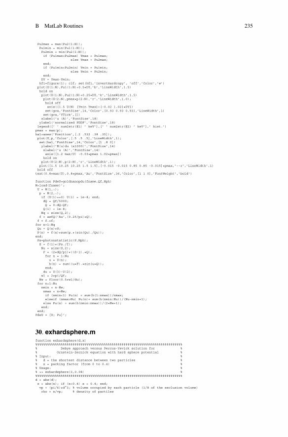
30. exhardsphere.mfunction exhardsphere(d,x)%%%%%%%%%%%%%%%%%%%%%%%%%%%%%%%%%%%%%%%%%%%%%%%%%%%%%%%%%%%%%%%%%%%%%%%%%%%% Debye approach versus Percus-Yevick solution for %% Ornstein-Zernick equation with hard sphere potential %% Input: %% d = the shortest distance between two particles %% x = packing factor (from 0 to 0.4) %% Usage: %% >> exhardsphere(3,0.08) %%%%%%%%%%%%%%%%%%%%%%%%%%%%%%%%%%%%%%%%%%%%%%%%%%%%%%%%%%%%%%%%%%%%%%%%%%%%d = abs(d);x = abs(x); if (x>0.4) x = 0.4; end;vp = (pi/6)*d^3; % volume occupied by each particle (1/8 of the exclusion volume)rho = x/vp; % density of partiles
236 B MatLab Routines
Umax = 5*d;du = d/100;U = 0:du:Umax;U(1)=1e-8;
Ud = U/d;Nu = size(U,2);aux1 = (1-x)^4;aux2 = -(1+0.5*x)^2 / aux1;aux1 = (1+2*x)^2 / aux1;C = (-0.5*x*aux1)*(Ud.*Ud.*Ud) - (6*x*aux2)*Ud - aux1;C(U>d) = 0;Qmax = 6 * (5*pi/2) / (2*d);
dq = Qmax/2000;Q = 0:dq:Qmax;Q(1) = 1e-8;Nq = size(Q,2);G = (4*pi*du)*C.*U;TFC = zeros(1,Nq);for n=1:Nqq = Q(n);TFC(n) = sum(G.*sin(q*U))/q;
end;S = 1./(1-rho*TFC);
Y = rho*(TFC.*TFC).*S;F = (dq/(2*pi*pi))*Y.*Q;invFTY = zeros(1,Nu);for n=1:Nu
u=U(n);invFTY(n) = sum(F.*sin(u*Q))/u;
end;g = invFTY + C + 1;g(U<d)=0;Qd = Q*d;T = tfsphere(Qd);Sp = 1-(8*rho*vp)*T;Smin = min(Sp);Smax = max(S);dS = Smax-Smin;
Smin = Smin-0.05*dS;Smax = Smax+0.05*dS;hf1=figure(1);clfset(hf1,’InvertHardcopy’, ’off’,’Color’,’w’)plot(Qd,Sp,’--k’,Qd,S,’r’,’LineWidth’,2)set(gca,’FontSize’,14,’Color’,[0.89 0.94 0.9],’FontName’,’Arial’,’LineWidth’,1)legend(’ Debye’,’ Percus-Yevick’,’Location’,’SouthWest’)
xlabel(’Qd’,’FontSize’,18);ylabel(’S(Q)’,’FontSize’,18);axis([0 max(Qd) Smin Smax])ha2=axes(’Position’,[.533 .251 .338 .4]);plot(Ud,g,’b’,’LineWidth’,2)set(ha2,’FontSize’,14,’Color’,[0.729 0.831 0.957],’FontName’,’Arial’,’LineWidth’,1)xlabel(’u/d’,’FontSize’,18)ylabel(’g(u)’,’FontSize’,18)
gmax = max(g);axis([0 max(Ud) 0 1.05*gmax])grid
function Z=tfsphere(u)u(u<=0)=1e-8;u3 = u.*u.*u;Z = 3*((sin(u)-u.*cos(u))./u3);
31. exkk.mfunction exkk(atom)%%%%%%%%%%%%%%%%%%%%%%%%%%%%%%%%%%%%%%%%%%%%%%%%%%%%%%%%%%%%%%%%%%%%%%%%%%%% Effects of exafs in the resonance amplitude: f’ +if’’ %% (model of 4 neighbors) %% Input: atom = element symbol, e.g. ’Fe’ %%%%%%%%%%%%%%%%%%%%%%%%%%%%%%%%%%%%%%%%%%%%%%%%%%%%%%%%%%%%%%%%%%%%%%%%%%%%dE = 2; % eVE=0:dE:70000; % eVNE = size(E,2);M = fpfpp(atom,E);nb = find(M(:,2)==min(M(:,2)));Eb = M(nb,1);K = E(nb:NE)-Eb; % kinetic energy of the photonelectron (eV)co = 0.512315; % units [Angstrom^{-1}][eV^{-1/2}]ke = co * sqrt(K);
ke(1) = 1e-6;Nk = size(ke,2);kmax = 5;aux = exp(2) / kmax^2;
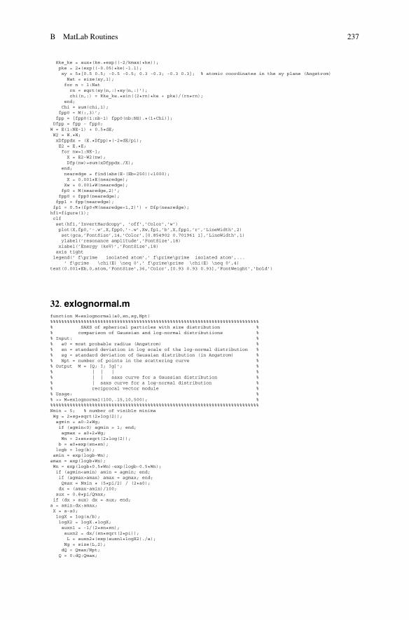
B MatLab Routines 237
Rke_ke = aux*(ke.*exp((-2/kmax)*ke));pke = 2*(exp((-0.05)*ke)-1.1);xy = 5*[0.5 0.5; -0.5 -0.5; 0.3 -0.3; -0.3 0.3]; % atomic coordinates in the xy plane (Angstrom)Nat = size(xy,1);for n = 1:Natrn = sqrt(xy(n,:)*xy(n,:)’);chi(n,:) = Rke_ke.*sin((2*rn)*ke + pke)/(rn*rn);
end;Chi = sum(chi,1);fpp0 = M(:,3)’;
fpp = [fpp0(1:nb-1) fpp0(nb:NE).*(1+Chi)];Dfpp = fpp - fpp0;W = E(1:NE-1) + 0.5*dE;W2 = W.*W;xDfppdx = (E.*Dfpp)*(-2*dE/pi);E2 = E.*E;for nw=1:NE-1;X = E2-W2(nw);Dfp(nw)=sum(xDfppdx./X);
end;nearedge = find(abs(E-(Eb+250))<1000);X = 0.001*E(nearedge);Xw = 0.001*W(nearedge);fp0 = M(nearedge,2)’;fpp0 = fpp0(nearedge);
fpp1 = fpp(nearedge);fp1 = 0.5*(fp0+M(nearedge+1,2)’) + Dfp(nearedge);hf1=figure(1);clfset(hf1,’InvertHardcopy’, ’off’,’Color’,’w’)plot(X,fp0,’-.w’,X,fpp0,’-.w’,Xw,fp1,’b’,X,fpp1,’r’,’LineWidth’,2)set(gca,’FontSize’,14,’Color’,[0.854902 0.701961 1],’LineWidth’,1)ylabel(’resonance amplitude’,’FontSize’,18)xlabel(’Energy (keV)’,’FontSize’,18)
axis tightlegend(’ f\prime isolated atom’,’ f\prime\prime isolated atom’,...
’ f\prime \chi(E) \neq 0’,’ f\prime\prime \chi(E) \neq 0’,4)text(0.001*Eb,0,atom,’FontSize’,36,’Color’,[0.93 0.93 0.93],’FontWeight’,’bold’)
32. exlognormal.mfunction M=exlognormal(a0,sn,sg,Npt)%%%%%%%%%%%%%%%%%%%%%%%%%%%%%%%%%%%%%%%%%%%%%%%%%%%%%%%%%%%%%%%%%%%%%%%%%%%% SAXS of spherical particles with size distribution %% comparison of Gaussian and log-normal distributiions %% Input: %% a0 = most probable radius (Angstrom) %% sn = standard deviation in log scale of the log-normal distribution %% sg = standard deviation of Gaussian distribution (in Angstrom) %% Npt = number of points in the scattering curve %% Output M = [Q; I; Ig]’; %% | | | %% | | saxs curve for a Gaussian distribution %% | saxs curve for a log-normal distribution %% reciprocal vector module %% Usage: %% >> M=exlognormal(100,.15,10,500); %%%%%%%%%%%%%%%%%%%%%%%%%%%%%%%%%%%%%%%%%%%%%%%%%%%%%%%%%%%%%%%%%%%%%%%%%%%%Nmin = 5; % number of visible minimaWg = 2*sg*sqrt(2*log(2));agmin = a0-2*Wg;if (agmin<0) agmin = 1; end;agmax = a0+2*Wg;Wn = 2*sn*sqrt(2*log(2));b = a0*exp(sn*sn);
logb = log(b);amin = exp(logb-Wn);amax = exp(logb+Wn);Wn = exp(logb+0.5*Wn)-exp(logb-0.5*Wn);if (agmin<amin) amin = agmin; end;if (agmax>amax) amax = agmax; end;Qmax = Nmin * (5*pi/2) / (2*a0);dx = (amax-amin)/100;
aux = 0.8*pi/Qmax;if (dx > aux) dx = aux; end;a = amin:dx:amax;X = a-a0;logX = log(a/b);logX2 = logX.*logX;auxn1 = -1/(2*sn*sn);auxn2 = dx/(sn*sqrt(2*pi));L = auxn2*(exp(auxn1*logX2)./a);Ng = size(L,2);dQ = Qmax/Npt;Q = 0:dQ:Qmax;
238 B MatLab Routines
Q(1) = 1e-8;aux = 4*pi/3;for n = 1:Ngaj = a(n);vj = aux * aj * aj * aj;u = aj*Q;x = vj*tfsphere(u);
Y(n,:) = x.*x;end;I = L*Y;v0 = aux * a0 * a0 * a0;u = a0 * Q;x = v0 * tfsphere(u);I0 = (x.*x);aux = -1.0 / (2*sg*sg);G = exp(aux *(X.*X));sumG = sum(G);G = (1/sumG)*G;Ig = G*Y;I = I*(1/max(I));
I0 = I0*(1/max(I0));Ig = Ig*(1/max(Ig));res = 100*abs(sum(abs(log(Ig)-log(I)))/sum(log(I)));x = -3*log(I(3)/I(2))/(Q(3)*Q(3)-Q(2)*Q(2));x = sqrt(x);y = -3*log(Ig(3)/Ig(2))/(Q(3)*Q(3)-Q(2)*Q(2));y = sqrt(y);a2 = a.*a;vp2 = (4*pi/3) * (a2.*a);vp2 = vp2.*vp2;
RgL = 0.6*sum(L.*vp2.*a2)/sum(L.*vp2);RgL = sqrt(RgL);RgG = 0.6*sum(G.*vp2.*a2)/sum(G.*vp2);RgG = sqrt(RgG);AsL = (4*pi)*sum(L.*a2);AsG = (4*pi)*sum(G.*a2);fprintf(’ log-normal: Rg = %3.1f(%3.1f)A, As = %5.3eA^2,fwhm=%3.1fA\n’,RgL,x,AsL,Wn)fprintf(’ Gaussian: Rg = %3.1f(%3.1f)A, As = %5.3eA^2,fwhm=%3.1fA\n’,RgG,y,AsG,Wg)
fprintf(’ residue = %5.3f\n’,res)Npt5 = 1:5:Npt;hf1=figure(1);clfset(hf1,’InvertHardcopy’, ’off’,’Color’,’w’)semilogy(Q,I0,’y--’,’LineWidth’,2)hold onsemilogy(Q(Npt5),I(Npt5),’-ro’,’MarkerFaceColor’,’w’,’MarkerSize’,4,’LineWidth’,1)semilogy(Q,Ig,’k’,’LineWidth’,1)hold offaxis([0 max(Q) 0.8*min(min([I; Ig])) 1.1])set(gca,’FontSize’,14,’Color’,[0.854902 0.701961 1])ylabel(’I(Q)/I(0)’,’FontSize’,18)xlabel(’Q (A^{-1})’,’FontSize’,18)
legend(’ sphere’,’ log-normal’,’ Gaussian’,4)M = [Q; I; Ig]’;ha1=axes(’Position’,[.48 .532 .38 .37]);hb=bar(0.1*a,L,1);hold on;plot(0.1*a,G,’k’,’LineWidth’,1);hold off;colormap coolset(ha1,’FontSize’,12,’Color’,[0.97 0.97 0.97])ylabel(’{\it p(a)}’)
xlabel(’radius, a (nm)’)axis tightlegend(’ log-n’,’ gaus’)
function Z=tfsphere(u)u3 = u.*u.*u;Z = 3*((sin(u)-u.*cos(u))./u3);
33. exlysozyme.mfunction exlysozyme%%%%%%%%%%%%%%%%%%%%%%%%%%%%%%%%%%%%%%%%%%%%%%%%%%%%%%%%%%%%%%%%%%%%%%%%%%%% Comparison of exact and approximate solutions for the SAXS curve %% Files required: %% - saxs2LYZ_0to180E20keV.dat (generated by routine saxs.c) %% - saxs2LYZ_0to40E8keV.dat (generated by routine saxs.c) %% - 2LYZ.ndu (generated by routine histogram.m) %% also available at http://xraybook.if.usp.br/ %% Secondary routines required: saxs.m and invftpofq.m %%%%%%%%%%%%%%%%%%%%%%%%%%%%%%%%%%%%%%%%%%%%%%%%%%%%%%%%%%%%%%%%%%%%%%%%%%%%M=saxs(’2LYZ.ndu’,2,80,0);M(:,2)=M(:,2)*(1/max(M(:,2)));Qmax = max(M(:,1));
B MatLab Routines 239
Pmin = min(M(:,2));S=load(’saxs2LYZ_0to180E20keV.dat’);smax = max(S(:,2));Ns=find(S(:,1)<=Qmax);ymin = S(max(Ns),2)/smax;if (Pmin<ymin) ymin=Pmin; end;X=M(:,1)*(0.25/pi);
fmQ = 193*asfQ(’N’,X)+613*asfQ(’C’,X)+185*asfQ(’O’,X)+10*asfQ(’S’,X);fmQ = fmQ.*fmQ;hf1=figure(1); clf; set(hf1,’InvertHardcopy’, ’off’,’Color’,’w’)semilogy(M(:,1),M(:,2),’-bo’,’MarkerFaceColor’,’w’,’MarkerSize’,6,’LineWidth’,1)hold onsemilogy(M(:,1),(fmQ.*M(:,2))/fmQ(1),’--b’,’LineWidth’,1.5)semilogy(S(:,1),S(:,2)/smax,’k’,’LineWidth’,1.5)hold offaxis([0 Qmax 0.9*ymin 1.1])
set(gca,’FontSize’,18,’Color’,[0.93 0.93 0.93],’YTick’,[0.001 0.01 0.1 1],’LineWidth’,1)xlabel(’Q (A^{-1})’,’FontSize’,18)ylabel(’P(Q) / P(0)’,’FontSize’,18)legend(’f_m^2(0), small angle’,’f_m^2(Q)’,’exact solution’,1)text(0.45,0.5,’2LYZ’,’FontSize’,36,’Color’,[0.855 0.702 1.0],’FontWeight’,’bold’)N=invftpofq(’saxs2LYZ_0to40E8keV.dat’,0.75,52,1000);H=load(’2LYZ.ndu’);n = size(H,1);
du = H(3,1)-H(2,1);Hsum = sum(H(2:n,2))*du;Hmax = max(H(2:n,2));hf2=figure(2); clf; set(hf2,’InvertHardcopy’, ’off’,’Color’,’w’)plot(H(2:n,1),H(2:n,2),’b’,’LineWidth’,1)hold onplot(N(:,1),Hsum*N(:,2),’--k’,’LineWidth’,1.5)hold offaxis([0 H(n,1) [-0.02 1.02]*Hmax])set(gca,’FontSize’,18,’Color’,[0.93 0.93 0.93],’LineWidth’,1)
xlabel(’u (A)’,’FontSize’,18)ylabel(’N(u)du’,’FontSize’,18)text(8,250,’ \leftarrow p(u)’,’Color’,’k’,’FontSize’,18)
34. exrdf.mfunction M=exrdf(R0,d,N)%%%%%%%%%%%%%%%%%%%%%%%%%%%%%%%%%%%%%%%%%%%%%%%%%%%%%%%%%%%%%%%%%%%%%%%%%%%% RDF according to the hard sphere model %% numerical simulation based on random distribution of positions %% Input: %% R0 = volume radius of the distribution (Angstrom) %% d = minimum separation distance between positions (Angstrom) %% 2N = approximated number of initial positions in the volume %% Output M = [U; g]’, g(u) in a n-by-2 array %% Usage: M=exrdf(100,2,4000); %%%%%%%%%%%%%%%%%%%%%%%%%%%%%%%%%%%%%%%%%%%%%%%%%%%%%%%%%%%%%%%%%%%%%%%%%%%%time=clock; fprintf(’ %1.0fh%1.0fm%1.0fs\n’,time(4:6))NN=N;d2 = d*d;R02 = R0*R0;R = R0*(2*rand(N,3)-1);R2 = sum(R.*R,2);
R = R(R2<=R02,:);N = size(R,1);for n=1:Nrn = R(n,:);for m=n+1:Nrmn = R(m,:) - rn;rmn2 = rmn * rmn’;if (rmn2<d2)R(m,:) = R(m,:) + 4*R0;
end;end;
end;R2 = sum(R.*R,2);R = R(R2<=R02,:);N = size(R,1);V = (4*pi/3)*R0^3;rho = N / V;
Umax = 2*R0;du = 0.1;U = 0:du:Umax;U(1) = 1e-8;Nu = size(U,2);p = zeros(1,Nu);R2 = sum(R.*R,2);Mj = find(R2<0.25*R02); % 0.25 => 50% of R0 or 0.49 => 70% of R0
Nj = size(Mj,1);for nn=1:Nj
n = Mj(nn);rn = R(n,:);
240 B MatLab Routines
for m=1:n-1rmn = R(m,:) - rn;k = fix(sqrt(rmn * rmn’)/du)+1;p(k) = p(k) + 1;
end;for m=n+1:Nrmn = R(m,:) - rn;k = fix(sqrt(rmn * rmn’)/du)+1;p(k) = p(k) + 1;
end;end;g = p./(4*pi*rho*Nj*du*(U.*U));M = [U; g]’;fprintf(’ N=%1.0f, n=%1.0f, Nj=%1.0f, rho=%10.8f\n’,NN,N,Nj,rho)time=clock; fprintf(’ %1.0fh%1.0fm%1.0fs\n’,time(4:6))
35. exrdffitting.mfunction exrdffitting(a,b)%%%%%%%%%%%%%%%%%%%%%%%%%%%%%%%%%%%%%%%%%%%%%%%%%%%%%%%%%%%%%%%%%%%%%%%%%%%% Nf x Ni curve adjusted by Nf = Nmax*[1-exp(-alpha*Ni)] %% Input: %% a,b = alpha values for the two data sets given below %% Usage: exrdffitting(0.7e-5,2.1e-5) %%%%%%%%%%%%%%%%%%%%%%%%%%%%%%%%%%%%%%%%%%%%%%%%%%%%%%%%%%%%%%%%%%%%%%%%%%%%% Data sets from routine exrdfd.m with d = 2 and 3, e.g. exrdf(100,d,N); %
N=[ 2 4 8 10 20 40 60 80 100 120 200]*1000;n(1,:)=[1013 2047 4098 5171 10065 19451 27886 35914 43662 50446 74620]; % d = 2n(2,:)=[1028 2019 3997 4864 9219 16403 22345 26913 31125 34530 44749]; % d = 3%-------------------------------------------------------------------------%R0 = 100;V = (4*pi/3) * R0^3;d = [2 3];vp = (pi/6)*(d.*d.*d);N = N * (pi/6);X=0:1000:110000;na = 1/a;Ya = na*(1-exp(-a*X));nb = 1/b;
Yb = nb*(1-exp(-b*X));fprintf(’ rho(2)=%5.3f/v_p e rho(3)=%5.3f/v_p\n’,(na/V)*vp(1),(nb/V)*vp(2))
hf1 = figure(1);clfset(hf1,’InvertHardcopy’,’off’,’Color’,’w’)plot(N,n(1,:),’bo’,N,n(2,:),’ks’,N,N,’--r’,’MarkerFaceColor’,’w’,’MarkerSize’,8,’LineWidth’,1.5)legend(’ d = 2A’,’ d = 3A’,’ reference: N_f = N_i’,2)hold onplot(X,Ya,’b’,X,Yb,’k’,’LineWidth’,2)hold offset(gca,’FontSize’,14,’Color’,[0.93 0.93 0.93],’LineWidth’,1)
axis tightxlabel(’N_i’,’FontSize’,18)ylabel(’N_f’,’FontSize’,18)
36. exrdfplot.mfunction exrdfplot%%%%%%%%%%%%%%%%%%%%%%%%%%%%%%%%%%%%%%%%%%%%%%%%%%%%%%%%%%%%%%%%%%%%%%%%%%%% Plot RDFs generated by the hard sphere model %% Required file: exrdfplot.dat %% File generated by routine exrdf.m (see text for details), and %% available at http://fap.if.usp.br/~morelhao/xrayphysicsbook.html %%%%%%%%%%%%%%%%%%%%%%%%%%%%%%%%%%%%%%%%%%%%%%%%%%%%%%%%%%%%%%%%%%%%%%%%%%%%S = load(’exrdfplot.dat’)’;U1 = S(1,:); g1 = S(2,:); % <-- exrdf(100,2,2e+5) with R’ = 50% of R0U2 = S(3,:); g2 = S(4,:); % <-- exrdf(100,3,2e+5) with R’ = 50% of R0U3 = S(5,:); g3 = S(6,:); % <-- exrdf(100,2,2e+5) with R’ = 70% of R0hf1 = figure(1);clfset(hf1,’InvertHardcopy’,’off’,’Color’,’w’)plot(U2,g2,’-ks’,’MarkerFaceColor’,’w’,’MarkerSize’,6,’LineWidth’,1.5)hold onplot(U1,g1,’-bo’,’MarkerFaceColor’,’w’,’MarkerSize’,6,’LineWidth’,1.5)hold offset(gca,’FontSize’,14,’Color’,[.87 .92 .98],’LineWidth’,1)axis([0 10 0 1.39])xlabel(’u (A)’,’FontSize’,18)
ylabel(’g(u)’,’FontSize’,18)legend(’ d = 3A’,’ d = 2A’)grid
B MatLab Routines 241
ha1=axes(’Position’,[.481 .24 .38 .38]);plot(U2,g2,’k’,U1,g1,’b’,’LineWidth’,2);hold onplot(U3,g3,’--b’,’LineWidth’,1)hold offset(ha1,’FontSize’,16,’Color’,[.97 .97 .97])ylabel(’g(u)’,’FontSize’,16)xlabel(’u (A)’,’FontSize’,16)
axis([0 150 0 1.39])text(50,1.1,’ \downarrow effect of finite ensemble’,’FontSize’,12)grid
37. exrlp3Dview.mfunction exrlp3Dview(L,T,vlevel,disc)%%%%%%%%%%%%%%%%%%%%%%%%%%%%%%%%%%%%%%%%%%%%%%%%%%%%%%%%%%%%%%%%%%%%%%%%%%%% Generates 3D visualization of reciprocal lattice nodes in thin crystal %% with rectangular or circular area %% Input: %% L = lateral dimension (nm) %% T = thickness (nm) %% vlevel = isosurface level value, between 0 and 1 %% disc = 1 for crystals with circular area, otherwise rectangular area %% Usage: exrlp3Dview(200,100,0.038,1) %%%%%%%%%%%%%%%%%%%%%%%%%%%%%%%%%%%%%%%%%%%%%%%%%%%%%%%%%%%%%%%%%%%%%%%%%%%%Nc = 6;dQ = 1 / 2^Nc;QrangeXY = (-1:dQ:1)*(40/L);QrangeZ = (-1:dQ:1)*(30/T);[Qx,Qy,Qz]=meshgrid(QrangeXY, QrangeXY, QrangeZ);Qx(Qx==0)=1e-8;
Qy(Qy==0)=1e-8;Qz(Qz==0)=1e-8;if (disc==1)R=1i*L/2;T=T/2;Nq = size(Qx,1);dphi = pi/500;phi=0:dphi:2*pi-dphi;cphi=cos(phi);cphi(cphi==0)=1e-8;Qxy = sqrt(Qx(:,:,1).*Qx(:,:,1)+Qy(:,:,1).*Qy(:,:,1));Wxy = zeros(Nq);
for n=1:Nqfor m=1:Nqa = Qxy(n,m)*cphi;x = a*R;x = exp(x).*(1-x)-1;x = x ./ (a.*a);Wxy(n,m) = sum(x)*dphi;
end;end;Wxy = (1/(pi*R*conj(R)))*Wxy;W = cat(3,Wxy,Wxy);for n=1:Nc, W = cat(3,W,W); end;W = cat(3,W,Wxy);
W = W.*sin(T*Qz)./(T*Qz);elseL=L/2;T=T/2;W = sin(L*Qx)./(L*Qx);W = W.*sin(L*Qy)./(L*Qy);
W = W.*sin(T*Qz)./(T*Qz);end;W = sqrt(W.*conj(W));hf1 = figure(1);clfset(hf1,’InvertHardcopy’,’off’,’Color’,’w’)P = patch(isosurface(Qx,Qy,Qz,W,vlevel),’FaceColor’,’red’,’EdgeColor’,’none’);isonormals(Qx,Qy,Qz,W,P)view(3)
daspect([1 1 1])axis tightcamlightcamlight(-80,-10)lighting phongset(gca,’FontSize’,14,’Color’,[0.97 0.97 0.97],’Box’,’on’,’LineWidth’,1,’FontName’,’Arial’)gridview(-30,25)
xlabel(’Q_X (nm^{-1})’,’FontSize’,18)ylabel(’Q_Y (nm^{-1})’,’FontSize’,18)zlabel(’Q_Z (nm^{-1})’,’FontSize’,18)
242 B MatLab Routines
38. exsgc.mfunction M=exsgc(atom,Emin,Emax,Np)%%%%%%%%%%%%%%%%%%%%%%%%%%%%%%%%%%%%%%%%%%%%%%%%%%%%%%%%%%%%%%%%%%%%%%%%%%%% Incoherent scattering cross-section (Compton), sg_C %% comparison of analytical x numerical solutions %% Input: %% atom = element symbol, from ’H’ to ’Cs’ (Z from 1 to 55) %% Emin,Emax = energy range from Emin to Emax (eV or keV) %% Np = number of points in the sg_C x E curve %% Output M = [E sg1 sg2] %% | | | %% | | cross-section (barn), analytical solution %% | cross-section (barn), numerical solution %% energy (keV) %% Secondary routines required: csfQ.m and sgcompton.m %% Usage: %% >> M=exsgc(’Ca’,1,20,50); %%%%%%%%%%%%%%%%%%%%%%%%%%%%%%%%%%%%%%%%%%%%%%%%%%%%%%%%%%%%%%%%%%%%%%%%%%%%Emin = abs(Emin); Emax = abs(Emax);if (Emax < Emin), E = Emax; Emax = Emin; Emin = E; end;if (Emin>500), Emin = 0.001*Emin; Emax = 0.001*Emax; end;if (Emin<1), Emin = 1; end;if (Emax>25), Emax = 25; end;if (Np<2), Np=2; end;dE = (Emax-Emin)/(Np-1);
E = Emin:dE:Emax;NE = size(E,2);rad = pi/180;re = 2.817940285e-15; % (m)hc = 12.3985; % (keV.A)invWL = E/hc;dtth = 0.2; % (deg)TTH = 0:dtth:180; % (deg)X = TTH * rad;dx = dtth * rad;
aux1 = pi * re * re * dx * 1e+28;SinG = sin(X);PSinG = (2-SinG.*SinG).*SinG;for nn = 1:NE
S = csfQ(atom,invWL(nn)*sin(0.5*X));M(nn,1) = E(nn);M(nn,2) = aux1*sum(PSinG.*(S(:,2)’));
end;S = sgcompton(atom,E);M(:,3) = S(:,2);hf1=figure(1);clfset(hf1,’InvertHardcopy’, ’off’,’Color’,’w’)plot(E,M(:,3),’k’,’LineWidth’,2)hold onplot(E,M(:,2),’bo’,’MarkerFaceColor’,’w’,’MarkerSize’,6,’LineWidth’,1.5)hold offset(gca,’FontSize’,14,’Color’,[0.854902 0.701961 1],’LineWidth’,1)ylabel(’\sigma_C (barn)’,’FontSize’,18)xlabel(’Energy (keV)’,’FontSize’,18)axis tight; grid
legend(’ analytical’,’ numerical’,4)n = round(0.5*NE);text(E(n),M(n,3),atom,’FontSize’,36,’Color’,[0.98 0.98 0.98],’FontWeight’,’bold’)
39. exsgr.mfunction M=exsgr(atom,Emin,Emax,Np)%%%%%%%%%%%%%%%%%%%%%%%%%%%%%%%%%%%%%%%%%%%%%%%%%%%%%%%%%%%%%%%%%%%%%%%%%%%% Coherent scattering cross-section (Rayleigh), sg_R %% comparison of analytical x numerical solutions %% Input: %% atom = element symbol, e.g. ’O’ %% Emin,Emax = energy range from Emin to Emax (eV or keV) %% Np = number of points in the sg_R x E curve %% Output M = [E sg1 sg2] %% | | | %% | | cross-section (barn), analytical solution %% | cross-section (barn), numerical solution %% energy (keV) %% Secondary routines required: asfQ.m and sgrayleigh.m %% Usage: %% >> M=exsgr(’O’,2,20,50); %%%%%%%%%%%%%%%%%%%%%%%%%%%%%%%%%%%%%%%%%%%%%%%%%%%%%%%%%%%%%%%%%%%%%%%%%%%%Emin = abs(Emin); Emax = abs(Emax);if (Emax < Emin) E = Emax; Emax = Emin; Emin = E; end;if (Emin>500) Emin = 0.001*Emin; Emax = 0.001*Emax; end;if (Emin<2) Emin = 2; end;if (Emax>70) Emax = 70; end;if (Np<2) Np=2; end;
B MatLab Routines 243
dE = (Emax-Emin)/(Np-1);E = Emin:dE:Emax;NE = size(E,2);rad = pi/180;re = 2.817940285e-15; % (m)hc = 12.3985; % (keV.A)invWL = E/hc;dtth = 0.2; % (deg)TTH = 0:dtth:180; % (deg)X = TTH * rad;dx = dtth * rad;aux1 = pi * re * re * dx * 1e+28;
Ntth = size(X,2);SinG = sin(X);PSinG = (2-SinG.*SinG).*SinG;for nn = 1:NE
f = asfQ(atom,invWL(nn)*sin(0.5*X));f = f.*f;M(nn,1) = E(nn);M(nn,2) = aux1*sum(PSinG.*f);
end;S = sgrayleigh(atom,E);M(:,3) = S(:,2);hf1=figure(1);clfset(hf1,’InvertHardcopy’, ’off’,’Color’,’w’)plot(E,M(:,3),’k’,’LineWidth’,2)hold onplot(E,M(:,2),’bo’,’MarkerFaceColor’,’w’,’MarkerSize’,6,’LineWidth’,1.5)hold offset(gca,’FontSize’,14,’Color’,[0.854902 0.701961 1],’LineWidth’,1)ylabel(’\sigma_R (barn)’,’FontSize’,18)xlabel(’Energy (keV)’,’FontSize’,18)axis tight; grid
legend(’ analytical’,’ numerical’,1)n = round(0.5*NE);text(E(n),M(n,3),atom,’FontSize’,36,’Color’,[0.98 0.98 0.98],’FontWeight’,’bold’)
40. exshell.mfunction S=exshell(a,b,rhoa,rhob)%%%%%%%%%%%%%%%%%%%%%%%%%%%%%%%%%%%%%%%%%%%%%%%%%%%%%%%%%%%%%%%%%%%%%%%%%%%% Pair distance distribution function (PDDF) in %% particles like hollow sphere %% Input: %% a and b, external and internal radius (Angstrom) %% rhoa: density for b < r < a %% rhob: density for 0 < r < b %% Output S = [U; pnu; p; ph]’; %% | | | | %% | | | PDDF via histogram %% | | PDDF via inverse FT %% | PDDF via numerical integral %% internal distances (Angstrom) %% Usage: %% >> S = exshell(500,375,2,-1); %%%%%%%%%%%%%%%%%%%%%%%%%%%%%%%%%%%%%%%%%%%%%%%%%%%%%%%%%%%%%%%%%%%%%%%%%%%%if (b==a) b = 0.5 * a; elseif (b>a) c = a; a = b; b = c; end;M=PdeQ(a,b,rhoa,rhob,5);Q = M(1,:);P0 = M(2,:);dQ = Q(3)-Q(2);Umax = 2.4*a;du = Umax/1000;U = 0:du:Umax;U(1) = 1e-6;Nu = size(U,2);
A = (dQ/(2*pi*pi))*(P0.*Q);for n=1:Nu
u = U(n);p(n) = sum(A.*sin(Q*u))*u;
end;pnu=pdeunum(U,a,b,rhoa,rhob);Nat = 4000;rand(’state’,sum(100*clock));X = 2*rand(Nat,3)-1;X2 = sum(X.*X,2);N = find(X2<=1);R = X(N,:);r = sqrt(X2(N));N = size(R,1);R = a*R;ps = rhoa*ones(1,N);
ps(r<=b/a)=rhob;ph=zeros(1,Nu);for n=1:N
244 B MatLab Routines
for m=n+1:ND = R(m,:)-R(n,:);d = sqrt(D*D’);k = floor(d/du)+1;ph(k) = ph(k)+ps(m)*ps(n);
end;end;ph = 2*ph;Nmax = find(pnu==max(pnu));pnumax = sum(pnu(Nmax-10:Nmax+10))/20;pmax = sum(p(Nmax-10:Nmax+10))/20;phmax = sum(ph(Nmax-10:Nmax+10))/20;pnu = pnu/pnumax;p = p/pmax;
ph = ph/phmax;N = 1:7:Nu;Nh = 1:5:Nu;hf1=figure(1);clfset(hf1,’InvertHardcopy’, ’off’,’Color’,’w’)bar(U(Nh),ph(Nh),’FaceColor’,[.87 .49 0],’EdgeColor’,’w’)hold onplot(U(N),p(N),’-ro’,’MarkerFaceColor’,’w’,’MarkerSize’,4,’LineWidth’,1)plot(U,pnu,’k’,’LineWidth’,1)hold offset(gca,’FontSize’,14,’Color’,[1 .97 .92])
axis tightylabel(’p(u)’,’FontSize’,18)xlabel(’u (A)’,’FontSize’,18)legend(’ hist.’,’ inv. FT’,’ num. vl.’)ha1=axes(’Position’,[.14 .532 .3 .37]);P0 = P0/max(P0);semilogy(Q,P0,’r’,’LineWidth’,2)set(ha1,’FontSize’,14,’Color’,[0.9 0.9 1])ylabel(’P(Q)’,’FontSize’,14)
xlabel(’Q (A^{-1})’,’FontSize’,14)axis([Q(1) max(Q) 0.9e-5 1.1])S = [U; pnu; p; ph]’;
function M=PdeQ(a,b,rhoa,rhob,Nmin)Qmax = Nmin * (5*pi/2) / (2*a);dQ = Qmax/2000;Q = 0:dQ:Qmax;Q(1) = 1e-8;Va = 4*pi*a*a*a/3;
Vb = 4*pi*b*b*b/3;F = (Va*rhoa) * tfsphere(Q*a) - (Vb*(rhoa-rhob)) * tfsphere(Q*b);P = F.*conj(F);M = [Q; P];
function Z=tfsphere(u)u3 = u.*u.*u;Z = 3*((sin(u)-u.*cos(u))./u3);
function M=pdeunum(U,a,b,rhoa,rhob)Rmax = 1.1*a;dr = Rmax/1000;R = 0:dr:Rmax;Nr = size(R,2);invw = 10 / dr;Y = rhoef(R,a,b,rhoa,rhob,invw);Nu = size(U,2);
rhoRdr = (pi*dr)*(R.*Y);for n=1:Nu
u = U(n);for m=1:Nrr = R(m);z1 = (r-u); z1 = z1*z1;z2 = (r+u); z2 = z2*z2;dz = (z2-z1) / 400;Z = z1:dz:z2;Yz = rhoef(sqrt(Z),a,b,rhoa,rhob,invw);A(m) = dz * sum(Yz);
end;C(n) = sum(rhoRdr.*A)/u;
end;M = C.*U.*U;
function Y = rhoef(R,a,b,rhoa,rhob,invw)Y = (1./(1 + exp(invw*(R - a)))).*((rhoa-rhob)./(1 + exp(invw*(b - R)))+rhob);
B MatLab Routines 245
41. exsphere.mfunction M=exsphere%%%%%%%%%%%%%%%%%%%%%%%%%%%%%%%%%%%%%%%%%%%%%%%%%%%%%%%%%%%%%%%%%%%%%%%%%%%% Scattering by uniform sphere %%%%%%%%%%%%%%%%%%%%%%%%%%%%%%%%%%%%%%%%%%%%%%%%%%%%%%%%%%%%%%%%%%%%%%%%%%%%uhalf = 1.8149;alpha = log(2)/uhalf^2;U = 0:0.01:20; U(1) = 1e-6;Y = tfsphere(U);
Y = Y.*Y;Z = exp(-alpha*(U.*U));hf1=figure(1);clfset(hf1,’InvertHardcopy’, ’off’,’Color’,’w’)plot(U,Z,’r--’,U,Y,’b’,[1.815],[0.5],’ko’,’LineWidth’,2,’MarkerFaceColor’,’w’,’MarkerSize’,9)set(gca,’FontSize’,14,’Color’,[0.854902 0.701961 1],’LineWidth’,1)xlabel(’Qa’,’FontSize’,18)
ylabel(’I(Qa) / I(0)’,’FontSize’,18)text(0.35,0.505,’ Qa = 1.815 \rightarrow’,’FontSize’,18)axis([0 5 0 1.01])ha2=axes(’Position’,[.48 .48 .4 .4]);plot(U,log10(Z),’r--’,U,log10(Y),’b’,’LineWidth’,1)set(ha2,’FontSize’,14,’Color’,[0.9 0.9 1])
xlabel(’Qa’)ylabel(’log(I)’)axis([0 20 -5 0.02])M = [U; Y; Z]’;
function Z=tfsphere(u);u3 = u.*u.*u;Z = 3*((sin(u)-u.*cos(u))./u3);
42. exwaterccd.mfunction exwaterccd(E,Qf,N)%%%%%%%%%%%%%%%%%%%%%%%%%%%%%%%%%%%%%%%%%%%%%%%%%%%%%%%%%%%%%%%%%%%%%%%%%%%% X-ray diffraction of liquid water on a CCD area detector %% Input: %% E = X-ray energy (keV) %% Qf = rec. vector module (1/Angstrom) limited by sample-ccd distance %% N > 999, diffraction pattern with statistic of N counts %% Secondary routines required: exwaterSofQ.m %% Usage: %% >> exwaterccd(12,4,5e+6) %%%%%%%%%%%%%%%%%%%%%%%%%%%%%%%%%%%%%%%%%%%%%%%%%%%%%%%%%%%%%%%%%%%%%%%%%%%%A = 300; % square screen detector of lateral size 2A (mm)pixel = 5; % pixel size (mm)if (E>500) E = 0.001*E; end; %%%%%%%%%%%%%%%%%%%%%%%%%%%%%%%%%%%Qfmax = E*sin(0.5*atan(30/5)); %---> % to limit Qf so that the minimum %if (Qf>Qfmax) Qf = Qfmax; end; % sample-ccd distance is D = 5 cm %M = exwaterSofQ(Qf,0)’; %%%%%%%%%%%%%%%%%%%%%%%%%%%%%%%%%%%Q = M(1,:);PS = M(2,:);D = A / tan(2*asin(Qf/E));
X = 0:pixel:A;Y = -A:pixel:0;Nx = size(X,2);twopi_wl = 2*pi*E/12.3985;for n=1:Nx
for m=1:Nxv = [X(n) Y(m) D];v = v / sqrt(v*v’);cg = v(3);v = v - [0 0 1];q = twopi_wl*sqrt(v*v’);
DQ = abs(Q-q);nn=find(DQ==min(DQ));I(m,n) = PS(nn(1))* cg*cg*cg; % to account for effective pixel size
end;end;beye=zeros(Nx);for n=1:Nxbeye(n,Nx+1-n) = 1;
end;I = [I*beye I];
I = [I; beye*I];if (N>999) I = photonstatistic(I,N); end;hf1=figure(1);clfset(hf1,’InvertHardcopy’, ’off’,’Color’,’w’)set(gca,’FontSize’,14,’Color’,’k’,’LineWidth’,1)imagesc([-A A],[-A A],I)blackbluemap = [zeros(1,64) 0:1/63:1; zeros(1,64) 0:1/63:1; 0:1/63:1 ones(1,64)]’;colormap(blackbluemap)axis image
246 B MatLab Routines
view(0,90)colorbar(’YColor’,’k’,’FontSize’,14,’Location’,’East’,’LineWidth’,1)
xlabel(’X (mm)’,’FontSize’,18)ylabel(’Y (mm)’,’FontSize’,18)text(0,0,200,’photons per pixel’,’FontSize’,16,’Rotation’,90)
43. exwaterSofQ.mfunction M=exwaterSofQ(Qf,prn)%%%%%%%%%%%%%%%%%%%%%%%%%%%%%%%%%%%%%%%%%%%%%%%%%%%%%%%%%%%%%%%%%%%%%%%%%%%% Interference function S(Q) from published RDF of water %% Input: %% Qf = rec. vector module (1/Angstrom), upper limit of S(Q) integral %% prn = 1 for graphic output (figure window) %% Output M=[Q; I]’; %% | | %% | normalized intensity, I(Q)/NI_{TH} = P(Q)S(Q) %% reciprocal vector module (1/Angstrom) %% Secondary routines required: asfQ.m %% Required files: gofuwater.dat %% File available at http://xraybook.if.usp.br/ %% Usage: %% >> M=exwaterSofQ(20,1); %%%%%%%%%%%%%%%%%%%%%%%%%%%%%%%%%%%%%%%%%%%%%%%%%%%%%%%%%%%%%%%%%%%%%%%%%%%%GofU=load(’gofuwater.dat’)’;U = GofU(1,:);g = GofU(2,:);clear GofU;g(g<0)=0;U(1) = 1e-8;du = U(3)-U(2);dq = Qf/1000;Q = 0:dq:Qf;Q(1) = 1e-8;Nq = size(Q,2);alpha = max(U)^3 / (3*sum(g.*U.*U)*du);
rho = 1e-24 * 6.022e+23 / 18 / alpha;Gudu = (4*pi*rho*du)*(g-1).*U;
for n=1:Nqq = Q(n);S(n) = 1 + sum(Gudu.*sin(q*U))/q;
end;S(S<0)=0;
f = asfQ(’O2-.’,(0.25/pi)*Q);f2 = f.*f;if (prn==1)hf1=figure(1);clfset(hf1,’InvertHardcopy’, ’off’,’Color’,’w’)plot(Q,S,’b’,’LineWidth’,2)set(gca,’FontSize’,14,’Color’,[0.93 0.93 0.93],’LineWidth’,1)hold onplot(Q,f2/f2(1),’--k’,’LineWidth’,1)hold offxlabel(’Q (A^{-1})’,’FontSize’,18)ylabel(’S(Q)’,’FontSize’,18)text(2.5,.4,’ \leftarrow P(Q)/P(0)’,’FontSize’,14,’Color’,’k’)axis([0 Qf 0 1.02*max(S)])
ha1=axes(’Position’,[.481 .282 .38 .38]);plot(U,g,’y’,’LineWidth’,2);set(ha1,’FontSize’,14,’Color’,[.85 .7 1])set(ha1,’XTick’,[2 3 4 5 6 7 8 9])ylabel(’g(u)’,’FontSize’,14)xlabel(’u (A)’,’FontSize’,14)axis([1.5 9.5 -.05 2.95])text(5,2,’H_2O’,’FontSize’,36,’Color’,[.93 .93 .93],’FontWeight’,’bold’)
gridend;M=[Q; f2.*S]’;
44. fpfpp.mfunction M=fpfpp(A,EE)%%%%%%%%%%%%%%%%%%%%%%%%%%%%%%%%%%%%%%%%%%%%%%%%%%%%%%%%%%%%%%%%%%%%%%%%%%%% Linear interpolation of tabuled values of %% atomic resonance amplitude, f’ and f" %% Input: %% A = element symbol, e.g. ’Se’ %% EE = energy values (m-by-n array) (eV) %% Output M = [E f’ f" sga] %% | | | | %% | | | absorption cross-section (barn) %% | | imaginary term (electron number) %% | real term (electron number) %
B MatLab Routines 247
% energy (eV) %% Routine available for download at http://xraybook.if.usp.br/ %%%%%%%%%%%%%%%%%%%%%%%%%%%%%%%%%%%%%%%%%%%%%%%%%%%%%%%%%%%%%%%%%%%%%%%%%%%%s=size(EE); NofE=s(1)*s(2);if (EE(NofE)<500), EE = 1000*EE; end;aux = 2000 * 2.818 * 12398.5;W = dispersion(atomnm(A));NofW = size(W,1);if (NofW == 1)disp([’ Element ’ A ’ unknown!!!’]);M = [0 0 0];return;
end;EE(EE<=0) = 0.1;M = zeros(NofE,4);for ne = 1:NofEE = EE(ne);nw = 1; ctr = 0;E2 = 0; fa1 = W(nw,2); fa2 = W(nw,3);while (nw <= NofW)E1 = E2; x = fa1; y = fa2;E2 = W(nw,1); fa1 = W(nw,2); fa2 = W(nw,3);if (E2 > E)fa1 = (fa1 - x) * (E - E1) / (E2 - E1) + x;fa2 = (fa2 - y) * (E - E1) / (E2 - E1) + y;nw = NofW; ctr = 1;end;nw = nw + 1;
end;if (ctr==0), fa1 = W(nw-1,2); fa2 = W(nw-1,3); end;
M(ne,:) = [E fa1 fa2 aux*fa2/E];end;
function nm=atomnm(A)% This function is available at the book’s webpage
function Z=dispersion(nm)% This function is available at the book’s webpage
45. fthofu.mfunction R=fthofu(N,d,cyl,fnum,prn)%%%%%%%%%%%%%%%%%%%%%%%%%%%%%%%%%%%%%%%%%%%%%%%%%%%%%%%%%%%%%%%%%%%%%%%%%%%% Fourier Transform of function h(u) for a volumetric ensemble of %% particles with anysotric correlations %% Input: %% N, the ensemble has nearly (2N+1)x(2N+1)x7 particles %% d, degree of disorder along the X direction, Da/a = 1 + d*(2*rand-1) %% cyl = 1 for cylindrical volume, otherwise rectangular volume %% fnum = 1, 2,... (ID number of the output file), %% 0 to suppress FT calculation and file saving %% prn = 0 to suppress graphic output %% Output R(n,:) = [X Y Z] 3D coordinates of the particles %% file with n-by-n array of FT{Cq(u)} values on detector pixels %% Usage: %% >> R = fthofu(2,0.2,1,1,1,1); %%%%%%%%%%%%%%%%%%%%%%%%%%%%%%%%%%%%%%%%%%%%%%%%%%%%%%%%%%%%%%%%%%%%%%%%%%%%a0 = 10; % average particle-to-particle distance (Angstrom)dy = 0.1*d;N = round(abs(N));NN = 2*N + 1;X = zeros(NN,NN,NN);Y = zeros(NN,NN,NN);Z = zeros(NN,NN,NN);X(:,:,1) = d*(2*rand(NN)-1);Y(:,:,1) = dy*(2*rand(NN)-1);
Z(:,:,1) = zeros(NN);h = 0;if (N>0)X(:,:,2) = X(:,:,1) + 1 + d*(2*rand(NN)-1);X(:,:,3) = X(:,:,1) - 1 + d*(2*rand(NN)-1);Y(:,:,2) = Y(:,:,1) + 1 + dy*(2*rand(NN)-1);Y(:,:,3) = Y(:,:,1) - 1 + dy*(2*rand(NN)-1);Z(:,:,2) = Z(:,:,1) + 1;Z(:,:,3) = Z(:,:,1) - 1;
h = [0 1 -1];if (N>1)
for n = 2:NX(:,:,2*n) = X(:,:,2*(n-1)) + 1 + d*(2*rand(NN)-1);X(:,:,2*n+1) = X(:,:,2*(n-1)+1) - 1 + d*(2*rand(NN)-1);Y(:,:,2*n) = Y(:,:,2*(n-1)) + 1 + dy*(2*rand(NN)-1);Y(:,:,2*n+1) = Y(:,:,2*(n-1)+1) - 1 + dy*(2*rand(NN)-1);Z(:,:,2*n) = Z(:,:,2*(n-1)) + 1;Z(:,:,2*n+1) = Z(:,:,2*(n-1)+1) - 1;h(2*n:2*n+1) = [n -n];
end;
248 B MatLab Routines
end;end;N0 = N+1;nn = 0;for n=1:NNfor m=1:NNfor p=1:NNnn = nn + 1;R(nn,:) = [X(N0-h(p),N0+h(m),n) Y(N0-h(p),N0-h(n),m) Z(N0+h(n),N0+h(m),p)];
end;end;
end;clear X Y Z;R = a0*R;if (cyl == 1)raio2 = max(max(R));raio2 = raio2*raio2;
R = R(sum(R.*R,2)<raio2,:);end;R = R(R(:,3).*R(:,3)<1000,:);if (fnum~=0)Nr = size(R,1);twopi_wl = 2*pi/1; % wavelength of 1 Angstrom (X-ray of 12.4 keV)A = 150; % square screen detector of lateral size 2A (mm)D = 600; % sample-detector distance (mm)pixel = 0.5; % pixel size (mm)X = -A:pixel:A;Y = A:-pixel:-A;Nx = size(X,2);
for n=1:Nx XX(n,:)=X; YY(:,n)=Y’; end;for n=1:Nxfor m=1:NxS = [XX(1,n) YY(m,1) D];S = S / sqrt(S*S’) - [0 0 1];Q(m,n,:) = twopi_wl*S;
end;end;
time=clock; fprintf(’ %2.0fh%2.0fm%2.0fs\n’,time(4:6))C = zeros(size(Q,1),size(Q,2));for n=1:Nrfor m=n+1:Nrr = R(m,:)-R(n,:);C = C + cos(Q(:,:,1)*r(1)+Q(:,:,2)*r(2)+Q(:,:,3)*r(3));
end;end;
C = (2/Nr)*C+1;time=clock; fprintf(’ %2.0fh%2.0fm%2.0fs\n’,time(4:6))if (prn~=0)surf(XX,YY,log(C))shading interpaxis imageset(gcf,’InvertHardcopy’,’off’,’Color’,’w’)set(gca,’ZTick’,[],’FontSize’,14,’Color’,[0.93 0.93 0.93],’LineWidth’,1)xlabel(’ X (mm)’,’FontSize’,18)ylabel(’ Y (mm)’,’FontSize’,18)zlabel(’log(I)’,’FontSize’,18)view(-14,30)
end;if (cyl == 1)
save([’fthofu_N’ num2str(N) ’d’ num2str(100*d) ’sphere’ num2str(fnum) ’.dat’],’C’,’-ascii’);else
save([’fthofu_N’ num2str(N) ’d’ num2str(100*d) ’square’ num2str(fnum) ’.dat’],’C’,’-ascii’);end;
end;
46. fthofuplotmap.mfunction fthofuplotmap%%%%%%%%%%%%%%%%%%%%%%%%%%%%%%%%%%%%%%%%%%%%%%%%%%%%%%%%%%%%%%%%%%%%%%%%%%%% Surface map of TF{h(u)} as a function of Qx and Qy %% Required file: fthofu_N8d20sphere1to20.dat %% File generated by routine fthofu.m, %% and available at http://xraybook.if.usp.br/ %%%%%%%%%%%%%%%%%%%%%%%%%%%%%%%%%%%%%%%%%%%%%%%%%%%%%%%%%%%%%%%%%%%%%%%%%%%%I = load(’fthofu_N8d20sphere1to20.dat’); I = I/max(max(I));A = 150; pixel = 0.5; D=600; % same values used in routine fthofu.mQ = 20*sin(0.5*atan((-A:pixel:A)/D)); % Qmax normalized by a0/(2*pi)for n=1:size(Q,2)Qx(n,:) = Q;Qy(:,n) = -Q’;
end;hf1 = figure(1);clfset(hf1,’InvertHardcopy’,’off’,’Color’,’w’)surf(Qx,Qy,log10(I))shading interpaxis image
B MatLab Routines 249
view(-14,30)set(gca,’Position’,[0.05 0.07 0.85 0.9],’LineWidth’,1)set(gca,’FontSize’,14,’Color’,[0.93 0.93 0.93])set(gca,’ZTick’,[],’DataAspectRatio’,[0.03 0.03 0.4],’YTick’,[-2 -1 0 1 2],’XTick’,[-2 -1 0 1 2])colormap(jet)colorbar(’XColor’,’k’,’FontSize’,14,’Location’,’East’,’LineWidth’,1)
xlabel(’n_x’,’FontSize’,18)ylabel(’n_y’,’FontSize’,18)text(2,0,0,’Log(FT\{h(u)\})’,’FontSize’,16,’Rotation’,90)
47. fthofuR.mfunction fthofuR(N,d,cyl)%%%%%%%%%%%%%%%%%%%%%%%%%%%%%%%%%%%%%%%%%%%%%%%%%%%%%%%%%%%%%%%%%%%%%%%%%%%% 3D plot of the ensemble of particles generated by routine fthofu.m %% Secondary routines required: fthofu.m %% Input parameters N, d, and cyl defined in the required routine %%%%%%%%%%%%%%%%%%%%%%%%%%%%%%%%%%%%%%%%%%%%%%%%%%%%%%%%%%%%%%%%%%%%%%%%%%%%a0 = 10; % same value used in routine fthofu.mR = (1/a0)*fthofu(N,d,cyl,0,0);hf1=figure(1); clf; set(hf1,’InvertHardcopy’, ’off’,’Color’,’w’)subplot(1,2,2)plot3(R(:,1),R(:,2),R(:,3),’ro’,’MarkerFaceColor’,’y’,’MarkerSize’,3,’LineWidth’,.6)axis imageaxis([-9 9 -9 9 -7 7])view(0,60)set(gca,’FontSize’,14,’Color’,’w’,’LineWidth’,1)set(gca,’ZTick’,[],’YTick’,[])xlabel(’X/a’,’FontSize’,14)hold onplot3([-8 -6],[-8 -8],[-6 -6],’r’,’LineWidth’,2)text(-6,-8,-6,’x’)plot3([-8 -8],[-8 -6],[-6 -6],’b’,’LineWidth’,2)text(-8,-6,-6,’y’)
plot3([-8 -8],[-8 -8],[-6 -4],’k’,’LineWidth’,2)text(-8,-8,-4,’z’)hold offsubplot(1,2,1)plot3(R(:,1),R(:,2),R(:,3),’ro’,’MarkerFaceColor’,’y’,’MarkerSize’,3,’LineWidth’,.6)axis imageaxis([-9 9 -9 9 -7 7])view(90,60)set(gca,’FontSize’,14,’Color’,’w’,’LineWidth’,1)set(gca,’XTick’,[],’ZTick’,[])ylabel(’Y/a’,’FontSize’,14)hold onplot3([6 8],[-8 -8],[-6 -6],’r’,’LineWidth’,2)text(8,-8,-6,’x’)plot3([6 6],[-8 -6],[-6 -6],’b’,’LineWidth’,2)text(6,-6,-6,’y’)
plot3([6 6],[-8 -8],[-6 -4],’k’,’LineWidth’,2)text(6,-8,-4,’z’)hold off
48. goldnano.mfunction M=goldnano(D,desord)%%%%%%%%%%%%%%%%%%%%%%%%%%%%%%%%%%%%%%%%%%%%%%%%%%%%%%%%%%%%%%%%%%%%%%%%%%%% Histogram of interatomic distances, or PDDF, in %% gold nanoparticles with crystalline structure %% Input: %% D = particle diameter (Angstrom) %% desord = atomic disorder in percentege (%) of the distance 2.88 A %% Output M = [U; p]’; %% | | %% | histogram (number of occurrences between u and u+du) %% interatomic distances (Angstrom) %% Usage: M = goldnano(20,5); %%%%%%%%%%%%%%%%%%%%%%%%%%%%%%%%%%%%%%%%%%%%%%%%%%%%%%%%%%%%%%%%%%%%%%%%%%%%if (D>100), disp(’ Warning!!! Delay time can be very long for D > 100 Angstroms’); end;a=4.0782; % lattice parameter (Angstrom) of gold fcc crystalsif (D<a), D = a; end;N = fix(D/a)+1;Nc = 0;for m=0:N-1for n=0:N-1for p=0:N-1Nc = Nc + 1;R(Nc,:) = [m n p]; % lattice points
end;
250 B MatLab Routines
end;end;if (Nc==0), Nc = 1; R(1,:) = [0 0 0]; end;R=a*R;X = a*[0 0 0; .5 .5 0; .5 0 .5; 0 .5 .5]; % atomic coordinates regarding each lattice point
Nx = size(X,1);for n=2:Nx
for m=1:NcR((n-1)*Nc+m,:) = R(m,:) + X(n,:);
end;end;Nat = size(R,1);Cm = sum(R(:,1))/Nat;X = R - Cm*ones(Nat,3);X2 = sum(X.*X,2);NN = X2<0.25*D*D;R = X(NN,:);Nat = size(R,1);R = R + (0.01*desord*a/sqrt(2))*(1-2*rand(Nat,3));
c0 = fix(clock);hora = [num2str(c0(4)) ’:’ num2str(c0(5)) ’:’ num2str(c0(6))];disp([’ goldnano started at ’ hora])
Umax=1.02*D;du = 0.01;U = 0:du:Umax;Nu = size(U,2);p=zeros(1,Nu);for n=1:Natfor m=n+1:Natr = R(n,:)-R(m,:);k=fix(sqrt(r*r’)/du)+1;p(k) = p(k) + 1;
end;end;
p = 2*p;p(1) = Nat;plot(U,p,’r’,’LineWidth’,2)M = [U; p]’;c1 = fix(clock);hora = [num2str(c1(4)) ’:’ num2str(c1(5)) ’:’ num2str(c1(6))];disp([’ goldnano ended at ’ hora])Dc = c1-c0;if (Dc(6)<0), Dc(6)=60+Dc(6); Dc(5)=Dc(5)-1; end;if (Dc(5)<0), Dc(5)=60+Dc(5); Dc(4)=Dc(4)-1; end;
if (Dc(4)<0), Dc(4)=24+Dc(4); end;hora = [num2str(Dc(4)) ’:’ num2str(Dc(5)) ’:’ num2str(Dc(6))];disp([’ Time delay ’ hora ’ (h:m:s)’])
49. histogram.mfunction M=histogram(fname,prn)%%%%%%%%%%%%%%%%%%%%%%%%%%%%%%%%%%%%%%%%%%%%%%%%%%%%%%%%%%%%%%%%%%%%%%%%%%%% Histogram of interatomic distances, or PDDF, of %% molecules catalogued in the Protein Data Bank %% Input: %% fname = pdb text file, *.pdb, or saved files *.ndu %% if *.pdb, it calculates the histogram and generate file *.ndu %% if *.ndu, it just plots the histogram %% prn = 0 to suppress graphic window %% Output M = [U; p]’; %% | | %% | histogram %% interatomic distances (Angstrom) %% Usage: M = histogrm(’2LYZ.pdb’,1); %%%%%%%%%%%%%%%%%%%%%%%%%%%%%%%%%%%%%%%%%%%%%%%%%%%%%%%%%%%%%%%%%%%%%%%%%%%%M = [0 0];n1 = regexp(fname,’.pdb’); n2 = regexp(fname,’.ndu’);if isempty([n1 n2]), disp(’ >>>> Unknown file type!!!’); return; end;fidin = fopen(fname,’r’);if (fidin==-1), disp([’ >>>> File ’ fname ’ not found!!!’]); return; end;if isempty(n1)M = load(fname);U = M(:,1)’;p = M(:,2)’;Nu = size(U,2);soma = sum(p);N = round(sqrt(soma));RgII = sqrt(0.5*sum(p.*U.*U)/soma);
RgI = 0;fclose(fidin);
elsefout = [fname(1:n1-1) ’.ndu’];fidin = fopen(fname,’r’);line = fgets(fidin);n = 0;while (line~=-1)switch line(1:5)
B MatLab Routines 251
case {’ATOM ’} % use "case {’ATOM ’,’HETAT’}" to read both "ATOM" and "HETATM" recordsn = n + 1;R(n,:) = sscanf(line(31:54),’%f’)’;A(n,:) = line(77:78);
end;line = fgets(fidin);
end;fclose(fidin);
N = size(R,1); Nchem = 0; AA = zeros(N,1); NA = 1;while ~isempty(NA)
n = NA(1);Mn = A(n,1)==A(:,1) & A(n,2)==A(:,2);Nchem = Nchem + 1;AA(Mn) = Nchem;Atom(Nchem,:) = A(n,:);NA = find(AA==0);
end;for n=1:Nchem, fprintf(’ %1.0f %s’,size(find(AA==n),1),Atom(n,:)); end;fprintf(’\n’);Umax = 0;for n=1:Nfor m=n+1:Nr = R(m,:)-R(n,:);r2 = r*r’;if (r2>Umax) Umax = r2; end;
end;end;
Umax = 1.02*sqrt(Umax);du = 0.01;U = 0:du:Umax;Nu = size(U,2);p=zeros(1,Nu);soma = 0;for n=1:Nfor m=n+1:Nr = R(m,:)-R(n,:);r2 = r*r’;soma = soma + r2;k = floor(sqrt(r2)/du)+1;p(k) = p(k)+1;
end;end;p = 2*p; p(1)=N;RgI = sqrt(soma)/N;RgII = sum(U.*U.*p)/sum(p);RgII = sqrt(0.5*RgII);M = [U; p]’;
save(fout,’M’,’-ascii’);end;if (prn~=0)hf1=figure(1); clf; set(hf1,’InvertHardcopy’, ’off’,’Color’,’w’)plot(U(2:Nu),p(2:Nu),’b’,’LineWidth’,1)axis([0 U(Nu) [-0.02 1.02]*max(p(2:Nu))])set(gca,’FontSize’,14,’Color’,[0.93 0.93 0.93])xlabel(’u (A)’,’FontSize’,18)
ylabel(’N(u)’,’FontSize’,18)end;fprintf(’ Protein: %s\n’,fname(1:find(fname==’.’)-1))if (RgI==0), fprintf(’ Nat = %1.0f, Rg = %3.1fA\n’,N,RgII);
else fprintf(’ Nat = %1.0f, Rg = %3.1f(%3.1f)A\n’,N,RgI,RgII);end;
50. invftpofq.mfunction M=invftpofq(fname,Qf,Umax,Nu)%%%%%%%%%%%%%%%%%%%%%%%%%%%%%%%%%%%%%%%%%%%%%%%%%%%%%%%%%%%%%%%%%%%%%%%%%%%% Inverse Fourier Transform of the molecule’s scattering power, P(Q) %% Input: %% fname = file with Q and P in columns 1 and 2 (Q values in Angstrom) %% Qf = upper limit to calculate the inverse FT %% Umax = maximum interatomic distance (Angstrom) %% Nu = number of ponts in the calculated PDDF %% Output M = [U; p]’; %% | | %% | PDDF %% interatomic distances (Angstrom) %% Usage: N=invftpofq(’saxs2LYZ_0a40E8keV.dat’,0.75,52,1000); %% File saxs2LYZ_0a40E8keV.dat from http://xraybook.if.usp.br/ %%%%%%%%%%%%%%%%%%%%%%%%%%%%%%%%%%%%%%%%%%%%%%%%%%%%%%%%%%%%%%%%%%%%%%%%%%%%S=load(fname)’;Q = S(1,:);P = S(2,:);Nq = size(Q,2);dQ = Q(3)-Q(2);if (Qf < Q(Nq))
252 B MatLab Routines
n = find(abs(Q-Qf)<=0.5*dQ);Q = S(1,1:n);P = S(2,1:n);
end;du = Umax/Nu;U = 0:du:Umax;Nu = size(U,2);aux = dQ / (2*pi*pi);for n = 1:Nuu = U(n);Qu = u*Q;p(n) = aux*sum(P.*Qu.*sin(Qu));
end;pint = sum(p)*du;p = (1/pint)*p;M=[U; p]’;
51. kdpcoordfrac.mfunction kdpcoordfrac(etaP,etaK,etaO,fname,p)%%%%%%%%%%%%%%%%%%%%%%%%%%%%%%%%%%%%%%%%%%%%%%%%%%%%%%%%%%%%%%%%%%%%%%%%%%%% KDP crystal data file with root-mean-square displacements %% Input: %% etaP, etaK, etaO: rms(Angstrom) for P, K, and O atoms %% p = 1 to save file fname.in %% Usage: kdpcoordfrac(0.15,0.15,0.15,’KDP15’,1) %% Source: http://www.crystallography.net/, cod ID: 9007582 %%%%%%%%%%%%%%%%%%%%%%%%%%%%%%%%%%%%%%%%%%%%%%%%%%%%%%%%%%%%%%%%%%%%%%%%%%%%etaP = etaP*etaP; etaK = etaK*etaK; etaO = etaO*etaO;P = [7.4521 7.4521 6.974 90.0 90.0 90.0]; % lattice parametersRf(1:4,:) = [0 0 0; 1/2 0 3/4; 1/2 1/2 1/2; 0 1/2 1/4]; % P atomsRf(5:8,:) = [0 0 1/2; 1/2 0 1/4; 1/2 1/2 0; 0 1/2 3/4]; % K atomsx = 0.1484; y = 0.0826; z = 0.1259;Rf(9:16,:) = [x, y, z; -x, -y, z; y, -x, -z; -y, x, -z;... % O atoms
-x + 1/2, y, -z + 3/4; x + 1/2, -y, -z + 3/4;...-y + 1/2, -x, z + 3/4; y + 1/2, x, z + 3/4];
Rf(17:24,:) = Rf(9:16,:)+0.5*ones(8,3);Nat = size(Rf,1);N = Rf>1;Rf(N) = Rf(N) - 1;N = Rf<0;Rf(N) = Rf(N) + 1;OcupFactor = ones(Nat,1);Bfactor = (8*pi*pi)*[etaP*ones(4,1); etaK*ones(4,1); etaO*ones(16,1)];Rf = [Rf OcupFactor Bfactor];SYM = [’P ’; ’K ’; ’O2-.’];A = [4 4 16];nn = size(A,2);L = A(1);for n=2:size(A,2), L = [L sum(A(1:n))]; end;nn=0;for n=1:size(L,2)LL(n,:) = [nn+1 L(n)];nn = L(n);
end;if (p == 1), fid = fopen([fname ’.in’], ’w’); else fid = 1; fprintf(’\n’); end;fprintf(fid,’%6.4f %6.4f %6.4f %7.4f %7.4f %7.4f\n’,P(1),P(2),P(3),P(4),P(5),P(6));for nn=1:size(A,2)at = SYM(nn,:);a = LL(nn,1); b = LL(nn,2);
for m=a:bfprintf(fid,’%s %6.4f %6.4f %6.4f %4.2f %6.3f\n’,at,Rf(m,1),Rf(m,2),Rf(m,3),OcupFactor(m),Bfactor(m));
end;end;if (p == 1), fclose(fid); else fprintf(’\n’); end;
52. kdphistcomp.mfunction kdphistcomp%%%%%%%%%%%%%%%%%%%%%%%%%%%%%%%%%%%%%%%%%%%%%%%%%%%%%%%%%%%%%%%%%%%%%%%%%%%% Variation in structure factor square modules with disorder %% Required files: KDP10E10000.sft and KDP15OxE10000.sft %% Files generated by routines diffraction.m and kdpcoordfrac.m, and %% available at http://xraybook.if.usp.br/ %% Secondary routines required: diffraction.m %%%%%%%%%%%%%%%%%%%%%%%%%%%%%%%%%%%%%%%%%%%%%%%%%%%%%%%%%%%%%%%%%%%%%%%%%%%%fname1 = ’KDP10E10000.sft’; %etaK=etaP=etaO=0.1 (reference)fname2 = ’KDP15OxE10000.sft’; %etaK=etaP=0.1; etaO=0.15;E = 10000; eta1 = 0.1; eta2 = 0.15;I1 = diffraction(E,fname1,0);I2 = diffraction(E,fname2,0);N = I2(:,1)==I1(:,1);Q12 = I2(N,1)’;
B MatLab Routines 253
p1 = I1(N,3)’;p1 = p1/max(p1);p2 = I2(N,3)’;p2 = p2/max(p2);Dp21 = zeros(size(Q12));N = p1>0.02;Dp21(N) = 100*(p1(N)-p2(N))./p1(N);Q = Q12(p1==max(p1));
aux = -(eta2^2-eta1^2);Y21 = 100*(1-exp(aux*(Q12.*Q12 - Q*Q)));
hf1=figure(1); clf; set(hf1,’InvertHardcopy’, ’off’,’Color’,’w’)plot(Q12,Dp21,’r’,Q12,Y21,’--k’,’LineWidth’,2)set(gca,’FontSize’,14,’Color’,[0.87 0.92 0.98],’Box’,’on’,’LineWidth’,1)axis tight
xlabel(’Q (A^{-1})’,’FontSize’,18)ylabel(’\Delta |F_{hkl}|^2 (%)’,’FontSize’,18)legend(’ \eta_O = 0.15A, \eta_P = \eta_K = 0.10A’,’ \eta_O = \eta_P = \eta_K = 0.15A’)
53. kdphistogram.mfunction kdphistogram%%%%%%%%%%%%%%%%%%%%%%%%%%%%%%%%%%%%%%%%%%%%%%%%%%%%%%%%%%%%%%%%%%%%%%%%%%%% Histograms of |Fhkl|^2 x Q for KDP with Debye-Waller factor %% Required files: KDP0E10000.sft, KDP10E10000.sft, KDP15E10000.sft, and %% KDP20E10000.sft %% Files generated by routines diffraction.m and kdpcoordfrac.m, and %% available at http://xraybook.if.usp.br/ %% Secondary routines required: diffraction.m %%%%%%%%%%%%%%%%%%%%%%%%%%%%%%%%%%%%%%%%%%%%%%%%%%%%%%%%%%%%%%%%%%%%%%%%%%%%E = 10000; % X-ray energy (eV) used to calculate files *.sfthf1=figure(1); clf; set(hf1,’InvertHardcopy’, ’off’,’Color’,’w’)I = diffraction(E,’KDP0E10000.sft’,0);Q = I(:,1)’;p = I(:,3)’;pmax = max(p);p = p/pmax;plot(Q,p,’w’,’LineWidth’,3)axis([0.98*min(Q) 1.02*max(Q) -0.02 1.02])set(gca,’FontSize’,14,’Color’,[0.85 0.7 1.0],’LineWidth’,1)xlabel(’Q (A^{-1})’,’FontSize’,18)
ylabel(’\Sigma|F_{hkl}|^2 (relative values)’,’FontSize’,18)hold onI = diffraction(E,’KDP10E10000.sft’,0);Q = I(:,1)’;p = I(:,3)’/pmax;plot(Q,p,’r’,’LineWidth’,3)I = diffraction(E,’KDP15E10000.sft’,0);Q = I(:,1)’;p = I(:,3)’/pmax;plot(Q,p,’y’,’LineWidth’,3)I = diffraction(E,’KDP20E10000.sft’,0);Q = I(:,1)’;
p = I(:,3)’/pmax;plot(Q,p,’b’,’LineWidth’,3)legend(’ \eta = 0’,’ \eta = 0.10 A’,’ \eta = 0.15 A’,’ \eta = 0.20 A’)plot(Q,ones(size(Q)),’--w’,’LineWidth’,1)aux = -0.1*0.1;plot(Q,exp(aux*Q.*Q),’--r’,’LineWidth’,1)aux = -0.15*0.15;plot(Q,exp(aux*Q.*Q),’--y’,’LineWidth’,1)aux = -0.2*0.2;
plot(Q,exp(aux*Q.*Q),’--b’,’LineWidth’,1)hold offtext(5.5,.85,’KDP’,’FontSize’,36,’Color’,[.93 .93 .93],’FontWeight’,’bold’)
54. kinematiclimit.mfunction Z=kinematiclimit(E,fname,H)%%%%%%%%%%%%%%%%%%%%%%%%%%%%%%%%%%%%%%%%%%%%%%%%%%%%%%%%%%%%%%%%%%%%%%%%%%%% Integrated reflectivity via recursive equations %% Input: %% E = energy (eV) or wavelength (Angstrom) %% fname = file *.in with crystal data information %% H = [h k l] reflection indexes %% Secondary routines required: rcdarwinprins.m %% Usage: Z=kinematiclimit(10000,’GaAs.in’,[1 1 1]); %%%%%%%%%%%%%%%%%%%%%%%%%%%%%%%%%%%%%%%%%%%%%%%%%%%%%%%%%%%%%%%%%%%%%%%%%%%%M = rcdarwinprins(E,fname,H,0,0);V = M(1);d = M(2);if (V>1000), N = [1 2]*2^8; else N = [1 2]*2^7; end;S=rcdarwinprins(E,fname,H,N(1),0).’;Idyn(1) = sum(S(2,:).*conj(S(2,:)))*(S(1,2)-S(1,1));S=rcdarwinprins(E,fname,H,N(2),0).’;
254 B MatLab Routines
Idyn(2) = sum(S(2,:).*conj(S(2,:)))*(S(1,2)-S(1,1));alpha = (Idyn(2)-Idyn(1))/(N(2)-N(1));Sd=rcdarwinprins(E,fname,H,2^30,0).’;maxIdyn = sum(Sd(2,:).*conj(Sd(2,:)))*(Sd(1,2)-Sd(1,1));Nkin = maxIdyn/alpha;dN = Nkin/12;N = [N (1:1:48)*dN];dN = Nkin/2;N = [N N(size(N,2))+(1:1:12)*dN];m = size(N,2);Idyn = [Idyn zeros(1,m-2)];for n=3:mS=rcdarwinprins(E,fname,H,N(n),0).’;Idyn(n) = sum(S(2,:).*conj(S(2,:)))*(S(1,2)-S(1,1));
end;Idyn = Idyn*(100/maxIdyn);
X = N*(d/10000);alpha = (Idyn(2)-Idyn(1))/(X(2)-X(1));Ikin = alpha*X;Nk = find(Ikin<120);DI = 100*(Ikin-Idyn)./Idyn;n = find(DI>10, 1 );if (n>1)Xc = ((X(n)-X(n-1))/(DI(n)-DI(n-1)))*(10-DI(n-1)) + X(n-1);
else Xc = d*Nkin/20000;end;Z = [X; Idyn]’;hf1=figure(1); clf; set(hf1,’InvertHardcopy’, ’off’,’Color’,’w’)plot(X,Idyn,’-bo’,X(Nk),Ikin(Nk),’k’,[Xc Xc],[0 alpha*Xc],’--k’,’LineWidth’,2)axis([0 max(X) 0 120])set(gca,’FontSize’,14,’Color’,[.97 .97 .97],’LineWidth’,1)xlabel(’thickness (\mum)’,’FontSize’,18)ylabel(’P_N/P_{\infty} (%)’,’FontSize’,18)legend(’ dynamical’,’ kinematic’)
fprintf(’ 10%% deviation at %6.3fum\n’, Xc)text(Xc,10,[’ \leftarrow ’ num2str(round(Xc*10)/10) ’\mum’],’FontSize’,18)ha2=axes(’Position’,[.47 .25 .4 .40]);X=Sd(1,:);Y = Sd(2,:).*conj(Sd(2,:));xc = sum(X.*Y)/sum(Y);range = sum(abs(X-xc).*Y)/sum(Y);Xmin = xc-3*range;
Xmax = xc+3*range;plot(X,Y,’-b’,’LineWidth’,2)axis([Xmin Xmax 0 1.02*max(Y)])set(ha2,’FontSize’,14,’Color’,[1 1 1],’FontName’,’Arial’,’LineWidth’,1)xlabel(’\Delta\theta (arcsec)’,’FontSize’,16)ylabel(’R(\theta)’,’FontSize’,16)nlabel=fname(1:find(fname==’.’)-1);
rlabel=[’(’ num2str(H(1)) ’,’ num2str(H(2)) ’,’ num2str(H(3)) ’)’];text(xc+0.7*range,0.75*max(Y),nlabel,’FontSize’,24,’Color’,[0.86 0.86 0.86],’FontWeight’,’bold’)text(xc+0.6*range,0.55*max(Y),rlabel,’FontSize’,24,’Color’,[0.86 0.86 0.86],’FontWeight’,’bold’)
55. lauemethod.mfunction lauemethod(fname,A,B,TH)%%%%%%%%%%%%%%%%%%%%%%%%%%%%%%%%%%%%%%%%%%%%%%%%%%%%%%%%%%%%%%%%%%%%%%%%%%%% Laue method %% Input: %% fname: file *.in with crystal data information (see sfactor.m) %% A = [A1,A2,A3] crystallographic direction aligned to the z axis %% B = [B1,B2,B3] reference direction in the xz plane %% TH = [thx,thy,thz] rotation matrix R=Rx(thx)Ry(thy)Rz(thz) %% Output file *.laue with list of hkl reflection power and %% spot coordinates on the X-ray film %% Secondary routines required: asfQ.m and fpfpp.m %% Usage: %% lauemethod(’spodumen.in’,[1 0 0],[0 0 1],[10 90 0]) %% lauemethod(’Si.in’,[1 1 1],[-1 -1 2],[0 0 0]) %%%%%%%%%%%%%%%%%%%%%%%%%%%%%%%%%%%%%%%%%%%%%%%%%%%%%%%%%%%%%%%%%%%%%%%%%%%%wlmin = 1; wlmax = 2; % continuous spectrum, constant intensity approach
% wavelength between wlmin and wlmax (Angstrom)Lg = 75; % half film width (mm)D = 50; % film radius (mm),e = [0 1 0]; % polarization, electric field vibration directionpix = .2; % film pixel (mm)sg = 2*pix; % size of diffraction spots, half width at 61% of the maximumrad = pi / 180;twopii = 2*pi*i;hc = 12398.5;c0 = fix(clock);code = [num2str(c0(1)) num2str(c0(2)) num2str(c0(3)) num2str(c0(4)) num2str(c0(5)) num2str(c0(6))];n = regexp(fname,’.in’);if isempty(n) disp(’ >>>> Unknown file type!!!’); return; end;fidin = fopen(fname,’r’);if (fidin==-1) disp([’ >>>> File ’ fname ’ not found!!!’]); return; end;
B MatLab Routines 255
fout = [fname(1:n-1) code ’.laue’];line = fgets(fidin);P = sscanf(line,’%f’)’;if (size(P,2)~=6) disp(’ >>>> Linha 1: a b c alpha beta gamma’); return; end;
n = 0;line = fgets(fidin);while (line~=-1)n = n + 1;w = find(line==’ ’); w = w(1);atm(n,:) = ’ ’;atm(n,1:w-1) = line(1:w-1);if isempty(regexp(’abcdefghijklmnopqrstuvwxyz’,atm(n,2)))atomsym(n,:)=[1 w-1];
else atomsym(n,:)=[2 w-1]; end;Rat(n,:) = sscanf(line(w+1:size(line,2)),’%f’)’;
line = fgets(fidin);end;fclose(fidin);Nat = n; Nchem = 0; AA = zeros(Nat,1); NA = find(AA==0);while ~isempty(NA)n = NA(1);M = find(atm(n,1)==atm(:,1) & atm(n,2)==atm(:,2) & atm(n,3)==atm(:,3) & atm(n,4)==atm(:,4));Nchem = Nchem + 1;AA(M) = Nchem;NA = find(AA==0);acod(Nchem,:) = atm(n,:);asym(Nchem,:) = atomsym(n,:);
end;clear atm atomsym;P(4:6) = P(4:6)*rad;cosphi = cos(P(6)) - cos(P(5))*cos(P(4));cosphi = cosphi / (sin(P(5))*sin(P(4)));sinphi = sqrt(1-cosphi*cosphi);a1 = P(1) * [sin(P(5)) 0 cos(P(5))];a2 = P(2) * [sin(P(4))*cosphi sin(P(4))*sinphi cos(P(4))];a3 = P(3) * [0 0 1];vecA = A(1)*a1 + A(2)*a2 + A(3)*a3;vecB = B(1)*a1 + B(2)*a2 + B(3)*a3;e3 = vecA/norm(vecA);e2 = cross(vecA,vecB);
e2 = e2/norm(e2);e1 = cross(e2,e3);M = [e1; e2; e3]’;thx = TH(1)*rad;thy = TH(2)*rad;thz = TH(3)*rad;Rx = [1 0 0; 0 cos(thx) -sin(thx); 0 sin(thx) cos(thx)];Ry = [ cos(thy) 0 sin(thy); 0 1 0; -sin(thy) 0 cos(thy)];
Rz = [cos(thz) -sin(thz) 0; sin(thz) cos(thz) 0; 0 0 1];R = Rx*Ry*Rz;MR = M*R’;a = a1*MR;b = a2*MR;c = a3*MR;a1r = cross(b,c);Vc = a1r*a’;a1r = a1r/Vc;a2r = cross(c,a)/Vc;a3r = cross(a,b)/Vc;hmax = floor(2.0 / (wlmin * norm(a1r)));kmax = floor(2.0 / (wlmin * norm(a2r)));lmax = floor(2.0 / (wlmin * norm(a3r)));H = [-hmax:hmax];K = [-kmax:kmax];
L = [-lmax:lmax];m = 0;for nh = 1:2*hmax+1for nk = 1:2*kmax+1
for nl = 1:2*lmax+1h = H(nh); k = K(nk); l = L(nl);q = h*a1r + k*a2r + l*a3r;if (q(3)<0)q2 = q*q’;wl = -2*q(3)/q2;if ((wl<wlmax) && (wl>wlmin))sp = wl*q + [0 0 1];z = D*tan(asin(sp(2)));if (z*z<Lg*Lg)m = m + 1;HKL(m,:) = [h k l];WL(m,1) = wl;Yf(m,1) = z;Xf(m,1) = D*atan2(sp(1),-sp(3));Fhkl2(m,1) = sfactorQ(Nchem,acod,asym,hc/wl,sqrt(q2),AA,twopii,Rat,[h k l]);
p = cross(sp,cross(e,sp));p = p * p’;Ahkl(m,1) = p*wl*Fhkl2(m)/q2;
end;end;
256 B MatLab Routines
end;end;
end;end;Nrefl = m;X = Ahkl;Nmax = [];while (sum(X)>0)NN = find(X==max(X));X(NN) = 0;Nmax = [Nmax; NN];
end;Nrefl = size(Nmax,1);HKL = HKL(Nmax,:);WL = WL(Nmax);Yf = Yf(Nmax);Xf = Xf(Nmax);Fhkl2 = Fhkl2(Nmax);Ahkl = Ahkl(Nmax);clear Nmax X;
invF2max = 100/max(Fhkl2);invAmax = 100/max(Ahkl);fidout = fopen(fout,’w’);fprintf(fidout,’\n %s, A = [%2d %2d %2d], B = [%2d %2d %2d], TH = [%5.3f %5.3f %5.3f]\n’,...
fname,A(1),A(2),A(3),B(1),B(2),B(3),TH(1),TH(2),TH(3));fprintf(fidout,’|-------------|-----------------|----------|--------------------------------|\n’);fprintf(fidout,’| h k l | |Fhkl|^2 | wl(A) | Phkl X(mm) Y(mm) |\n’);fprintf(fidout,’|-------------|-----------------|----------|--------------------------------|\n’);for m=1:Nreflfprintf(fidout,’| %3d %3d %3d | %7.1f(%5.1f%%) | %8.6f | %9.1f %9.3f %9.3f |\n’,HKL(m,1),HKL(m,2),
HKL(m,3),...Fhkl2(m),invF2max*Fhkl2(m),WL(m),Ahkl(m),Xf(m),Yf(m));
end;fprintf(fidout,’|-------------|-----------------|----------|--------------------------------|\n’);fclose(fidout);
Nx = floor(pi*D/pix);Ny = floor(Lg/pix);perimeter = Nx*pix;width = Ny*pix;Z = zeros(2*Ny+1,2*Nx+1);for m=1:Nreflnx = fix(Xf(m)/pix)+Nx+1;ny = fix(Yf(m)/pix)+Ny+1;Z(ny,nx) = Z(ny,nx) + Ahkl(m);
end;Ng = floor(10*sg/pix);
Xg = (-Ng:Ng)*pix;Xg = Xg.*Xg;for nx=1:2*Ng+1for ny=1:2*Ng+1
Xg2(ny,nx) = Xg(ny) + Xg(nx);end;
end;G = (1/(sg*sg*2*pi))*exp((-1/(2*sg*sg))*Xg2);Zg = [zeros(2*Ny+1+2*Ng,Ng) [zeros(Ng,2*Nx+1); Z; zeros(Ng,2*Nx+1)] zeros(2*Ny+1+2*Ng,Ng)];for nx=1:2*Nx+1for ny=1:2*Ny+1
Z(ny,nx) = sum(sum(G.*Zg(ny:2*Ng+ny,nx:2*Ng+nx)));end;
end;hf1=figure(1); clf; set(hf1,’InvertHardcopy’, ’off’,’Color’,’w’)imagesc(perimeter*[-1 1],width*[-1 1],log10(Z+1))axis imageset(gca,’YDir’,’normal’,’FontName’,’Arial’,’FontSize’,14,’LineWidth’,1)colormap jet;colorbar(’FontSize’,14,’Location’,’EastOutside’,’LineWidth’,1)
ylabel(’film width (mm)’,’FontSize’,18)xlabel(’film length (mm)’,’FontSize’,18)text(1.274*perimeter,-width/3,5000,’Log(I) (arb. units)’,’FontSize’,14,’Rotation’,90)
function F2 = sfactorQ(Nchem,acod,asym,E,Q,AA,twopii,R,H)for n=1:Nchemaux = fpfpp(acod(n,1:asym(n,1)),E);fres(n) = aux(2)+1i*aux(3);
end;x = 0.5*Q;x2 = x*x;F = 0;for n=1:Nchemfn = asfQ(acod(n,1:asym(n,2)),x) + fres(n);NA=find(AA==n)’;
F = F + fn*sum(exp(twopii*(R(NA,1:3)*H’)).*R(NA,4).*exp((-x2)*R(NA,5)));end;F2 = F*conj(F);
B MatLab Routines 257
56. orientcryst.mfunction orientcryst(wl,P,A,B,TH,H)%%%%%%%%%%%%%%%%%%%%%%%%%%%%%%%%%%%%%%%%%%%%%%%%%%%%%%%%%%%%%%%%%%%%%%%%%%%%%%%%%%%%%%%%%%%%%%%%%%%%% Alignment of Single Crystals %% Input: %% wl = wavelength (Angstrom) or energy (eV) %% P = [a b c alpha beta gamma] parameters of the unit cell (in Angstrom and degree) %% A = [A1,A2,A3] crystallographic direction parallel to the z axis (incident beam) %% B = [B1,B2,B3] reference direction in the xz plane %% TH = [thx,thy,thz], orientation matrix R=Rx(thx)Ry(thy)Rz(thz) %% H = [h k l] reflection indexes, use TH = [1] or [] to orient reflection hkl with %% chi or phi alignment, respectively %% Usage: %% orientcryst(1.540562,[9.4620 8.3920 5.2210 90.00 110.180 90.00],[1 0 0],[0 1 0],[0 0 0],[0 0 2]) %% orientcryst(1.540562,[9.4620 8.3920 5.2210 90.00 110.180 90.00],[1 0 0],[0 1 0],[],[0 0 2]) %% orientcryst(1.540562,[9.4620 8.3920 5.2210 90.00 110.180 90.00],[1 0 0],[0 1 0],[1],[0 0 2]) %%%%%%%%%%%%%%%%%%%%%%%%%%%%%%%%%%%%%%%%%%%%%%%%%%%%%%%%%%%%%%%%%%%%%%%%%%%%%%%%%%%%%%%%%%%%%%%%%%%%%rad = pi / 180;if (wl < 1000), E = 12398.5 / wl; else E = wl; wl = 12398.5 / E; end;if isempty(P), return; end;nm = size(P);if (nm(1)*nm(2)==1)P(1:3) = P(1)*ones(1,3);P(4:6) = [90 90 90];
elseif (nm(1)*nm(2)==2)P(1:3) = [P(1) P(1) P(2)];P(4:6) = [90 90 90];
end;P(4:6) = P(4:6)*rad;cosphi = cos(P(6)) - cos(P(5))*cos(P(4));cosphi = cosphi / (sin(P(5))*sin(P(4)));sinphi = sqrt(1-cosphi*cosphi);a1 = P(1) * [sin(P(5)) 0 cos(P(5))];a2 = P(2) * [sin(P(4))*cosphi sin(P(4))*sinphi cos(P(4))];a3 = P(3) * [0 0 1];vecA = A(1)*a1 + A(2)*a2 + A(3)*a3;vecB = B(1)*a1 + B(2)*a2 + B(3)*a3;e3 = vecA/norm(vecA);e2 = cross(vecA,vecB);e2 = e2/norm(e2);
e1 = cross(e2,e3);M = [e1; e2; e3]’;a = a1*M;b = a2*M;c = a3*M;a1r = cross(b,c);Vc = a1r*a’;a1r = a1r/Vc;a2r = cross(c,a)/Vc;a3r = cross(a,b)/Vc;
Q = H(1,1)*a1r + H(1,2)*a2r + H(1,3)*a3r;modQ = norm(Q);if (size(TH,2)==3)thx = TH(1)*rad;thy = TH(2)*rad;thz = TH(3)*rad;Rx = [1 0 0; 0 cos(thx) -sin(thx); 0 sin(thx) cos(thx)];Ry = [ cos(thy) 0 sin(thy); 0 1 0; -sin(thy) 0 cos(thy)];Rz = [cos(thz) -sin(thz) 0; sin(thz) cos(thz) 0; 0 0 1];
R = Rx*Ry*Rz;elsethbragg = asin(0.5*wl*modQ);if isempty(TH)
thy = pi/2-acos(Q(3)/modQ) + thbragg;x = Q(1); y = Q(2);thz = -atan2(y,x);Rz = [cos(thz) -sin(thz) 0; sin(thz) cos(thz) 0; 0 0 1];Ry = [ cos(thy) 0 sin(thy); 0 1 0; -sin(thy) 0 cos(thy)];R = Ry*Rz;fprintf(’ Chi alignment: R = RyRz, thz = %9.4f, thy = %9.4f,
thBragg = %9.4f\n’,thz/rad,thy/rad,thbragg/rad)else
thy = acos(Q(1)/modQ) + thbragg;x = Q(2); y = Q(3);thx = 0.5*pi - atan2(y,x);Rx = [1 0 0; 0 cos(thx) -sin(thx); 0 sin(thx) cos(thx)];Ry = [ cos(thy) 0 sin(thy); 0 1 0; -sin(thy) 0 cos(thy)];R = Ry*Rx;fprintf(’ Phi alignment: R = RyRx, thx = %9.4f, thy = %9.4f,
thBragg = %9.4f\n’,thx/rad,thy/rad,thbragg/rad)end;
end;MR = M*R’;a = a1*MR;b = a2*MR;c = a3*MR;a1r = cross(b,c);Vc = a1r*a’;
258 B MatLab Routines
a1r = a1r/Vc;a2r = cross(c,a)/Vc;a3r = cross(a,b)/Vc;
Q = H(1,1)*a1r + H(1,2)*a2r +H(1,3)*a3r;O = [0 0 0];d = a + b + c;A = b + c;B = a + c;C = a + b;D = 0.5*d;modD = 1.5*norm(D);
vecA = modD*e3*MR;vecB = modD*e1*MR;Q = modD*(Q/norm(Q));hf1 = figure(1); clf; set(hf1,’InvertHardcopy’,’off’,’Color’,’w’)vector(O,a,-D,’b’,1,’ a’);hold onvector(O,b,-D,’b’,1,’ b’);vector(O,c,-D,’b’,1,’ c’);
vector(O,[0 0 1.5*modD],[0 0 0],’r’,2,’\uparrow X-rays’);vector(O,Q,[0 0 0],’m’,2,’ Q’);vector(O,vecB,[0 0 0],’k’,2,’ B’);vector(O,vecA,[0 0 0],’k’,2,’ A’);vector(B,a,-D,’b’,1,[]);vector(B,c,-D,’b’,1,[]);vector(B,d,-D,’b’,1,[]);vector(C,a,-D,’b’,1,[]);vector(C,b,-D,’b’,1,[]);vector(C,d,-D,’b’,1,[]);
vector(A,b,-D,’b’,1,[]);vector(A,c,-D,’b’,1,[]);vector(A,d,-D,’b’,1,[]);plot3(modD*[1 -1 -1 -1 -1 1],modD*[-1 -1 1 1 -1 -1],modD*[1 1 1 -1 -1 -1],’k’,’LineWidth’,1 )plot3(modD*[-1 -1],modD*[-1 -1],modD*[1 -1],’k’,’LineWidth’,1 )plot3(-D(1),-D(2),-D(3),’b.’)axis imageaxis(modD*[-1 1 -1 1 -1 1])hold offtext(0,0,0,’O’)set(gca,’FontSize’,18,’Color’,[0.97 0.97 0.97],’LineWidth’,1)gridxlabel(’X (A)’,’FontSize’,18)
ylabel(’Y (A)’,’FontSize’,18)zlabel(’Z (A)’,’FontSize’,18)view(164,18)
function vector(A,B,T,cor,linha,nome)V = [(A+T)’ (B+T)’];plot3(V(1,:),V(2,:),V(3,:),cor,’LineWidth’,linha)if ~isempty(nome)text(V(1,2),V(2,2),V(3,2),nome,’Color’,cor,’FontSize’,18)
end;
57. pdbcoordfrac.mfunction pdbcoordfrac(fname,OP)%%%%%%%%%%%%%%%%%%%%%%%%%%%%%%%%%%%%%%%%%%%%%%%%%%%%%%%%%%%%%%%%%%%%%%%%%%%% To generate crystal data information files (*.in) from %% *.pdb file format (see http://www.wwpdb.org/) %% Input: %% fname = *.pdb file %% OP = space group number %% Output save file *.in as described in routine sfactor.m %% Usage: %% >> pdbcoordfrac(’1TRZ.pdb’,146) %%%%%%%%%%%%%%%%%%%%%%%%%%%%%%%%%%%%%%%%%%%%%%%%%%%%%%%%%%%%%%%%%%%%%%%%%%%%n = regexp(fname,’.pdb’);if isempty(n), disp(’ >>>> Unknown file type!!!’); return; end;fout = [fname(1:n-1) ’.in’];fidin = fopen(fname,’r’);if (fidin==-1), disp([’ >>>> File ’ fname ’ not found!!!’]); return; end;line = fgets(fidin); n=0; m=0;while (line~=-1)switch line(1:5)case {’CRYST’}
P = sscanf(line(7:54),’%f’)’;case {’SCALE’}
m = m + 1;SC(m,:) = sscanf(line(11:40),’%f’)’;
case {’ATOM ’,’HETAT’}n = n + 1;Rf(n,:) = [(SC*sscanf(line(31:54),’%f’))’ sscanf(line(55:66),’%f’)’];A(n,:) = line(77:78);
end;line = fgets(fidin);
end;fclose(fidin);
B MatLab Routines 259
N = size(Rf,1); Nchem = 0; Achem = zeros(N,1); NA = 1;while ~isempty(NA)
n = NA(1);Mn = find(A(n,1)==A(:,1) & A(n,2)==A(:,2));Nchem = Nchem + 1;OCF(Nchem) = sum(Rf(Mn,4));Achem(Mn) = Nchem;if (A(n,1)~=’ ’), Atom(Nchem,:) = [A(n,1) lower(A(n,2))];
else Atom(Nchem,:) = [A(n,2) ’ ’];end;NA = find(Achem==0);
end;fprintf(’ Atoms in the asymmetric unit with occupation factor (...)\n’)for n=1:Nchemx = size(find(Achem==n),1);fprintf(’ %1.0f(%4.2f)%s’,x,OCF(n)/x,Atom(n,:))
end;fprintf(’\n’);fid = fopen(fout,’w’);fprintf(fid,’%6.4f %6.4f %6.4f %6.4f %6.4f %6.4f\n’,P(1),P(2),P(3),P(4),P(5),P(6));for n=1:NR = symop(OP,Rf(n,1:3));for m=1:size(R,1)
fprintf(fid,’%s %8.4f %8.4f %8.4f %6.3f %6.2f\n’,Atom(Achem(n),:),R(m,1),R(m,2),R(m,3),Rf(n,4),Rf(n,5));end;
end;fclose(fid);
function R=symop(OP,Rf)X=Rf(1); Y=Rf(2); Z=Rf(3);switch OP
case {4}R(1,:) = [X,Y,Z; -X,Y+1/2,-Z];
case {18}R(1,:) = [X,Y,Z; -X,-Y,Z; -X+1/2,Y+1/2,-Z; X+1/2,-Y+1/2,-Z];
case {96}R = [ X, Y, Z; -X, -Y, Z+1/2; -Y+1/2,X+1/2,Z+3/4; Y+1/2,-X+1/2, Z+1/4;
-X+1/2,Y+1/2,-Z+3/4; X+1/2,-Y+1/2,-Z+1/4; Y, X, -Z; -Y, -X,-Z+1/2];case {146}R = [ X, Y, Z; -Y, X-Y, Z; -X+Y, -X, Z;
X+2/3,Y+1/3,Z+1/3; -Y+2/3,X-Y+1/3,Z+1/3; -X+Y+2/3,-X+1/3,Z+1/3;X+1/3,Y+2/3,Z+2/3; -Y+1/3,X-Y+2/3,Z+2/3; -X+Y+1/3,-X+2/3,Z+2/3];
case {169}R = [ X, Y, Z; -Y, X-Y,Z+1/3; -X+Y,-X,Z+2/3;
-X,-Y,Z+1/2; Y,-X+Y,Z+5/6; X-Y, X,Z+1/6];case {197}R = [ X, Y,Z; -X,-Y, Z; -X,Y,-Z; X,-Y,-Z; Z, X, Y; Z,-X,-Y;
-Z,-X,Y; -Z, X,-Y; Y,Z, X; -Y, Z,-X; Y,-Z,-X; -Y,-Z, X];R = [R; R+0.5*ones(12,3)];
% case {...} % include other "case" to add an operation symmetry% from 230 space groups, see "International Tables for% Crystallography (2006). Vol. A, ch. 7.1, pp. 112-717
otherwise, R = [X,Y,Z];end;
58. photonsonpsp.mfunction I=photonsonpsp(thx,thy,thz,D,L,pixel,wl,N)%%%%%%%%%%%%%%%%%%%%%%%%%%%%%%%%%%%%%%%%%%%%%%%%%%%%%%%%%%%%%%%%%%%%%%%%%%%% Intensity pattern with statistic of N counts %% Input: %% thx, thy, thz, D, L, pixel, and wl defined in routine benzeneonpsp.m %% N = number of photons (counts) scattered on the film %% Output: I = counts on the pixel array %% Secondary routines required: benzeneonpsp.m and photonstatistic.m %% Usage: %% >> I = photonsonpsp(30,0,90,50,200,2,20000,1e+4); %%%%%%%%%%%%%%%%%%%%%%%%%%%%%%%%%%%%%%%%%%%%%%%%%%%%%%%%%%%%%%%%%%%%%%%%%%%%dz = pixel;n = floor(2*L/dz);LimZ = 0.5*n*dz;Y=benzeneonpsp(thx,thy,thz,D,L,pixel,wl,0);I=photonstatistic(Y,N)+1;hf1=figure(1);clfset(hf1,’InvertHardcopy’, ’off’,’Color’,’w’)imagesc([-LimZ LimZ],[-1 1]*D*pi,log10(I))axis imageset(gca,’FontSize’,14,’LineWidth’,1,’YTick’,[-150 -100 -50 0 50 100 150])colormap(hot)colorbar(’XColor’,’k’,’YColor’,’k’,’FontSize’,14,’Location’,’East’,’LineWidth’,1)
xlabel(’film width (mm)’,’FontSize’,18)ylabel(’film length (mm)’,’FontSize’,18)text(0,0,5000,’Log(número de fótons / pixel)’,’FontSize’,18,’Rotation’,90,’Color’,’k’)
260 B MatLab Routines
59. photonstatistic.mfunction Z=photonstatistic(M,N)soma = sum(sum(M));M = M*(1/soma);Z = zeros(size(M));for np = 1:Naux = 0; photon = rand; nn = 0;while (aux<photon)nn = nn + 1;aux = aux + M(nn);
end;Z(nn) = Z(nn) + 1;
end;
60. polymer.mfunction M=polymer(Nm,jct,sofq)%%%%%%%%%%%%%%%%%%%%%%%%%%%%%%%%%%%%%%%%%%%%%%%%%%%%%%%%%%%%%%%%%%%%%%%%%%%% Scattering curve S(Q) of a polymer or %% its gyration radius Rg %% Input: %% Nm = number of monomers in the chain %% jct = 1 for limited junction, otherwise free junction (RW model) %% sofq = 0 for gyration radius %% Output M = [Q; S]’, S(Q) curve if sofq ~= 0 %% M = Rg2, mean square radius (Angstrom^2) if sofq = 0 %% Secondary routines required: polymerchain.m %% Usage: %% >> M = polymer(2000,0,1); %%%%%%%%%%%%%%%%%%%%%%%%%%%%%%%%%%%%%%%%%%%%%%%%%%%%%%%%%%%%%%%%%%%%%%%%%%%%L = 1.54; % monomer length (Angstrom)R = 10*polymerchain(Nm,jct,0);Rg2theo = Nm*L*L/6;if (sofq~=0)Qmax = 18/sqrt(Rg2theo);dq = Qmax/100;Q = 0:dq:Qmax;Q(1) = 1e-8;Nq = size(Q,2);S = zeros(1,Nq);for jj=1:Nmrj = R(jj,1);for kk = jj+1:Nmrjk = R(kk,1)-rj;S = S + cos(rjk*Q);
end;end;S = 2*S;
M = [Q; S]’;else M = sum(sum(R.*R))/Nm;end;
61. polymerchain.mfunction R=polymerchain(Nm,jct,prn)%%%%%%%%%%%%%%%%%%%%%%%%%%%%%%%%%%%%%%%%%%%%%%%%%%%%%%%%%%%%%%%%%%%%%%%%%%%% Virtual chain of monomers with free or limited junction %% Input: %% Nm = number of monomers in the chain %% jct = 1 for limited junction, otherwise free junction (RW model) %% prn = 0 to suppress graphic window %% Output R, array of 3D coordinates of the monomers %% Usage: %% >> R = polymerchain(1000,0,1); %%%%%%%%%%%%%%%%%%%%%%%%%%%%%%%%%%%%%%%%%%%%%%%%%%%%%%%%%%%%%%%%%%%%%%%%%%%%L = 0.154; % monomer length (nm)if (jct==1)
phi = [-1 0 1]*(2*pi/3);T = [(71+2*(2*rand(Nm,1)-1))*(pi/180) phi(fix(2.99999999999*rand(Nm,1))+1)’];
elseT = [pi*rand(Nm,1) (2*pi)*rand(Nm,1)];
end;R(1,:) = [0 0 0];M = eye(3);for n=1:Nmst = sin(T(n,1));ct = cos(T(n,1));sp = sin(T(n,2));cp = cos(T(n,2));M = [ct*cp ct*sp -st; -sp cp 0; st*cp st*sp ct]*M;
R(n+1,:) = R(n,:) + L*M(3,:);end;
B MatLab Routines 261
Nm = Nm + 1;rc = sum(R)/Nm;R(:,1) = R(:,1)-rc(1);R(:,2) = R(:,2)-rc(2);R(:,3) = R(:,3)-rc(3);if (prn~=0)n=24;Ncor = 0.02*(0:1:n)’;n = n + 1;C = [zeros(n,1) zeros(n,1) 1-Ncor;
Ncor zeros(n,1) 0.5*ones(n,1);0.5*ones(n,1) zeros(n,1) 0.5-Ncor;
0.5+Ncor zeros(n,1) zeros(n,1)];x = Nm/100;hf1 = figure(1); clf; set(hf1,’InvertHardcopy’,’off’,’Color’,’w’)plot3(R(1,1),R(1,2),R(1,3),’b.’)hold onfor n=2:Nmplot3(R(n-1:n,1),R(n-1:n,2),R(n-1:n,3),’Color’,C(fix((n-1)/x)+1,:),’LineWidth’,1.2)
end;plot3(R(Nm,1),R(Nm,2),R(Nm,3),’r.’)hold offset(gca,’FontSize’,14,’Color’,[0.93 0.93 0.93],’Box’,’on’,’LineWidth’,1)axis imageaxis tight; gridxlabel(’X (nm)’,’FontSize’,18)ylabel(’Y (nm)’,’FontSize’,18)
zlabel(’Z (nm)’,’FontSize’,18)end;
62. polymerkratky.mfunction polymerkratly%%%%%%%%%%%%%%%%%%%%%%%%%%%%%%%%%%%%%%%%%%%%%%%%%%%%%%%%%%%%%%%%%%%%%%%%%%%% Comparison of structural function S(Q) for systems of %% polymers with different weight %% Required files: ’polymer2k_1to500.dat’, ’polymer6k_1to500.dat’, and %% ’polymer10k_1to500.dat’ %% Files generated by routine polymersystem.m, and available at %% http://xraybook.if.usp.br/ %%%%%%%%%%%%%%%%%%%%%%%%%%%%%%%%%%%%%%%%%%%%%%%%%%%%%%%%%%%%%%%%%%%%%%%%%%%%fna = ’polymer2k_1to500.dat’; Nma = 2000;fnb = ’polymer6k_1to500.dat’; Nmb = 6000;fnc = ’polymer10k_1to500.dat’; Nmc = 10000;M = load(fna)’;Qa=M(1,:);Sa=M(2,:);M = load(fnb)’;Qb=M(1,:);Sb=M(2,:);
M = load(fnc)’;Qc=M(1,:);Sc=M(2,:);L = 1.54; % monomer length (Angstrom)Rg2a = 770;Rg2b = 2200;Rg2c = 3730;Ua = Rg2a*(Qa.*Qa);
Ub = Rg2b*(Qb.*Qb);Uc = Rg2c*(Qc.*Qc);Ya = 2*(exp(-Ua)-1+Ua)./(Ua.*Ua);Ya(1) = 1;Ya = Ya*Sa(1);Yb = 2*(exp(-Ub)-1+Ub)./(Ub.*Ub);Yb(1) = 1;Yb = Yb*Sb(1);
Yc = 2*(exp(-Uc)-1+Uc)./(Uc.*Uc);Yc(1) = 1;Yc = Yc*Sc(1);hf1 = figure(1);clfset(hf1,’InvertHardcopy’,’off’,’Color’,’w’)N=1:1:size(Qa,2);Ur=sqrt(Ua(N));
Q2 = Qa(N).^2;plot(Ur,Sa(N).*Q2,’-bo’,Ur,Ya(N).*Q2,’--k’,’MarkerFaceColor’,’w’,’MarkerSize’,6,’LineWidth’,1.5)N=1:1:size(Qb,2);Ur=sqrt(Ub(N));Q2 = Qb(N).^2;hold onplot(Ur,Sb(N).*Q2,’-md’,Ur,Yb(N).*Q2,’--k’,’MarkerFaceColor’,’w’,’MarkerSize’,6,’LineWidth’,1.5)N=1:1:size(Qc,2);Ur=sqrt(Uc(N));Q2 = Qc(N).^2;
plot(Ur,Sc(N).*Q2,’-rs’,Ur,Yc(N).*Q2,’--k’,’MarkerFaceColor’,’w’,’MarkerSize’,6,’LineWidth’,1.5)hold offset(gca,’FontSize’,14,’Color’,[0.894 0.941 0.902],’LineWidth’,1)
262 B MatLab Routines
xlabel(’QR_g’,’FontSize’,18)ylabel(’N_m^2Q^2S(Q)’,’FontSize’,18)text(13,47000,’N_m = 10000’,’FontSize’,18,’Color’,’r’)
text(13,26000,’N_m = 6000’,’FontSize’,18,’Color’,’m’)text(13,5000,’N_m = 2000’,’FontSize’,18,’Color’,’b’)axis([0 17.5 0 5.9e+4])
63. polymerRg.mfunction polymerRg(N,Nm)%%%%%%%%%%%%%%%%%%%%%%%%%%%%%%%%%%%%%%%%%%%%%%%%%%%%%%%%%%%%%%%%%%%%%%%%%%%% Statistical distribution of gyration radius for %% free and limited junction models %% Ensemble: N polymers with Nm monomers each %% Secondary routines required: polymer.m %% Usage: %% >> polymerRg(1000,2000) %%%%%%%%%%%%%%%%%%%%%%%%%%%%%%%%%%%%%%%%%%%%%%%%%%%%%%%%%%%%%%%%%%%%%%%%%%%%for n=1:NRa(n,1)=polymer(Nm,0,0);Rb(n,1)=polymer(Nm,1,0);
end;Ra = 0.01*Ra;Rb = 0.01*Rb;du = 20/8;Umax = max(Ra);Ua = 0:du:Umax;p = zeros(size(Ua));for n=1:Nk = fix(Ra(n)/du)+1;p(k) = p(k) + 1;
end;pa = (100/du) * p / sum(p);Rg2a = sum(Ra)/N;xa=find(abs(Ua-Rg2a)<du);N = size(Rb,1);Umax = max(Rb);Ub = 0:du:Umax;p = zeros(size(Ub));for n=1:Nk = fix(Rb(n)/du)+1;p(k) = p(k) + 1;
end;pb = (100/du) * p / sum(p);Rg2b = sum(Rb)/N;xb=find(abs(Ub-Rg2b)<du);hf1 = figure(1);clfset(hf1,’InvertHardcopy’,’off’,’Color’,’w’)plot([Rg2a Rg2a],[0 pa(xa(1))],’--k’,Ua,pa,’-k.’,’LineWidth’,2)hold onplot([Rg2b Rg2b],[0 pb(xb(1))],’--b’,Ub,pb,’-b.’,’LineWidth’,2)hold offset(gca,’FontSize’,14,’Color’,[0.93 0.93 0.93],’LineWidth’,1)xlabel(’R_g^2 (nm^2)’,’FontSize’,18)ylabel(’number of occurrences (%/nm^2)’,’FontSize’,18)
text(Rg2a,pa(xa(1)),’ \leftarrow free’,’FontSize’,18,’Color’,’k’)text(Rg2b,pb(xb(1)),’ \leftarrow limited’,’FontSize’,18,’Color’,’b’)axis tight
64. polymersystem.mfunction polymersystem(fname,Nm,jct,N)%%%%%%%%%%%%%%%%%%%%%%%%%%%%%%%%%%%%%%%%%%%%%%%%%%%%%%%%%%%%%%%%%%%%%%%%%%%% Scattering curve S(Q) by systems of polymers %% Input %% fname = output file name %% Nm = number of monomers in each polymer %% jct = 1 for limited junction, otherwise free junction (RW model) %% N = number of polymers in the system %% Output file fname with the S(Q) curve for the system of N polymers %% Secondary routines required: polymer.m %% Usage: %% >> polymersystem(’polymer2k_1a500.dat’,2000,0,500) %%%%%%%%%%%%%%%%%%%%%%%%%%%%%%%%%%%%%%%%%%%%%%%%%%%%%%%%%%%%%%%%%%%%%%%%%%%%for n=1:NM=polymer(Nm,jct,1);Y(:,n)=M(:,2);
end;S = sum(Y,2)/N;M = [M(:,1) S];save(fname,’M’,’-ascii’)
B MatLab Routines 263
65. quartzgofu.mfunction M=quartzgofu(E,tthmax,conv)%%%%%%%%%%%%%%%%%%%%%%%%%%%%%%%%%%%%%%%%%%%%%%%%%%%%%%%%%%%%%%%%%%%%%%%%%%%% RDF obtained by inverse FT of the interference function S(Q) in %% a cluster of disordered alpha-quartz %% Input: %% E, energy (keV) %% tthmax, maximum scattering angle (from 10 to 180 deg) %% conv = 1 to convolve g(u) with a rectangular function of unit area %% and width 2*pi/Qf %% Output M=[U; g]’; g(u) curve %% Secondary routines required: quartzIofQ.m %% Required files: clusterN12d2_1to10.dat and clusterN12d2gofu.dat %% from http://xraybook.if.usp.br/ %% Usage: M=quartzgofu(30,180,0); %%%%%%%%%%%%%%%%%%%%%%%%%%%%%%%%%%%%%%%%%%%%%%%%%%%%%%%%%%%%%%%%%%%%%%%%%%%%if (E>100), E = 0.001*E; end; wl = 12.3985/E;Qmax = 4*pi/wl;if (tthmax<10), disp(’Wide angle scattering, from 10 to 180 deg!!!’); return;elseif (tthmax>180), tthmax = 180;end;Qf = Qmax*sind(0.5*tthmax);S=quartzIofQ(wl,0,’clusterN12d2_1to10.dat’);Nq = S(:,1)<=Qf;Q = S(Nq,1)’;I = S(Nq,2)’;S = S(Nq,3)’;GofU = load(’clusterN12d2gofu.dat’);U = GofU(:,1)’;g0 = GofU(:,2)’;hf1=figure(1); clf; set(hf1,’InvertHardcopy’, ’off’,’Color’,’w’)plot(U,g0,’-ro’,’LineWidth’,1,’MarkerFaceColor’,’y’,’MarkerSize’,5)
set(gca,’FontSize’,14,’FontName’,’Arial’,’Color’,[0.93 0.93 0.93],’LineWidth’,1)xlabel(’u (A)’,’FontSize’,18)ylabel(’g(u)’,’FontSize’,18)U=U(U>0.1);Nu = size(U,2);Np = Q>0.7;Q = Q(Np); S=S(Np);rho = 9/113.01;dQ = (Q(3)-Q(2))/(2*pi*pi*rho);
g = zeros(1,Nu);for n=1:Nu
u=U(n);g(n) = 1+(dQ/u)*sum((S-1).*Q.*sin(Q*u));
end;if (conv==1)du = U(3)-U(2);wdt = 2*pi/Qf;Nw = floor(0.5*wdt/du);
gexp = zeros(1,Nu);for n=1:Nunmin = n-Nw;nmax = n+Nw;if (nmin<1), gexp(n) = sum(g(1:nmax))/nmax;elseif (nmax>Nu), gexp(n) = sum(g(nmin:Nu))/(Nu-nmin+1);
else gexp(n) = sum(g(nmin:nmax))/(2*Nw+1);end;
end;g=gexp;
end;hold onplot(U,g,’k’,’LineWidth’,1.5)hold offgmax = max(g0);aux = max(g);if (aux>gmax), gmax=aux; end;gmin = min(g);if (gmin>0), gmin=0; end;dg = 0.02*(gmax-gmin);axis([0.1 13.1 gmin-dg gmax+dg])
TTh = 2*asind(Q/Qmax);Imin = min(I);Imax = max(I);DI = 0.02*(Imax-Imin);ha2=axes(’Position’,[.4 .45 .48 .43]);plot(TTh,I,’k’,’LineWidth’,2)set(ha2,’FontSize’,14,’FontName’,’Arial’,’Color’,[1 1 1],’LineWidth’,1)gridxlabel(’2\theta (deg)’);ylabel(’intensity (cps)’);axis([TTh(1) 0.2*max(TTh) Imin-DI Imax+DI])N = Q>2.12;alpha = 0.75*Imax/max(I(N));hold on;plot(TTh(N),alpha*I(N)+0.25*Imax,’b’,’LineWidth’,2)
hold offtext(0.15*max(TTh),0.5*Imax,[’ x’ num2str(0.1*round(10*alpha))],’FontSize’,18,’Color’,’b’)
M = [U; g]’;
264 B MatLab Routines
66. quartzIofQ.mfunction M=quartzIofQ(wl,prn,fname)%%%%%%%%%%%%%%%%%%%%%%%%%%%%%%%%%%%%%%%%%%%%%%%%%%%%%%%%%%%%%%%%%%%%%%%%%%%% Calculates S(Q) and I(Q) for clusters of disordered alpha-quartz %% Input: %% wl = wavelength (Angstrom) or energy (eV) %% prn = 0 to suppress graphic window %% fname = file of RDFs in a n-by-5 array format (see quartzrdf.m), e.g. %% ’clusterN12dX_1to10.dat’ from http://xraybook.if.usp.br/ %% Output M=[Q; I; S]’; n-by-3 arrary for I(Q) and S(Q) curves %% Secondary routines required: asfQ.m, fpfpp.m, and csfQ.m %% Usage: M=quartzIofQ(1.54,1,’clusterN12d20_1to10.dat’); %% Note: resonant and Compton scatterings are included. %%%%%%%%%%%%%%%%%%%%%%%%%%%%%%%%%%%%%%%%%%%%%%%%%%%%%%%%%%%%%%%%%%%%%%%%%%%%if (wl < 100), E = 12398.5 / wl; else E = wl; wl = 12398.5 / E; end;Qmax = 4*pi/wl;S=load(fname);U = S(:,1)’;Uc = 21.07; y = exp(-5.2e-5*(U-Uc).^2.505); y(U<Uc)=1;y = 1 - y; % <--| correction explained in routine quartzrdfplot.mgsi = S(:,2)’+y; gox = S(:,3)’+y; gsiox = S(:,4)’+y; goxsi = S(:,5)’+y;Vc = 113.01; % unit cell volume (Angstrom^3) containing 3Si and 6OrhoSi = 3/Vc;
rhoOx = 6/Vc;rho = rhoSi + rhoOx;dQ = Qmax/5000;Q = 0:dQ:Qmax;Q(1) = 1e-8;Nq = size(Q,2);
Z = fpfpp(’Si’,E);fSi = asfQ(’Si’,(0.25/pi)*Q) + Z(1,2) + 1i*Z(1,3);Z = fpfpp(’O’,E);fOx = asfQ(’O’,(0.25/pi)*Q) + Z(1,2) + 1i*Z(1,3);ASi = real(fSi.*conj(fSi));AOx = real(fOx.*conj(fOx));fm2 = (1/3)*ASi + (2/3)*AOx;ASi = (rhoSi*rhoSi)*ASi(1);AOx = (rhoOx*rhoOx)*AOx(1);ASiOx = (rhoSi*rhoOx)*real(fSi(1).*conj(fOx(1)));AOxSi = (rhoOx*rhoSi)*real(fOx(1).*conj(fSi(1)));
w2 = (ASi + AOx + ASiOx + AOxSi);g = (ASi*gsi + AOx*gox + ASiOx*gsiox + AOxSi*goxsi)/w2;
du = U(3)-U(2);% GofU = [U; g0]’; save(’clusterN12d2gofu.dat’,’GofU’,’-ascii’); % uncomment to save the total RDFaux = 4*pi*du*rho;S=zeros(1,Nq);for n=1:Nqq = Q(n);S(n) = 1 + (aux/q)*sum((g - 1).*sin(q*U).*U);
end;Np = Q>0.7;Q = Q(Np); S=S(Np); fm2=fm2(Np);TTh = 2*asind(Q/Qmax);C = (1/3)*csfQ(’Si’,(0.25/pi)*Q)+(2/3)*csfQ(’C’,(0.25/pi)*Q);
I = fm2.*S + C(:,2)’;M=[Q; I; S]’;if (prn~=0)Imin = min(I);Imax = max(I);DI = 0.02*(Imax-Imin);hf1=figure(1);clfset(hf1,’InvertHardcopy’, ’off’,’Color’,’w’)plot(TTh,I,’k’,’LineWidth’,2)set(gca,’FontSize’,14,’FontName’,’Arial’,’Color’,[0.93 0.93 0.93],’LineWidth’,1)xlabel(’2\theta (deg)’,’FontSize’,18);ylabel(’intensity (cps)’,’FontSize’,18);
axis([TTh(1) 180 Imin-DI Imax+DI])Nu = U>0.1;ha2=axes(’Position’,[.45 .4 .43 .48]);plot(U(Nu),g(Nu),’k’,’LineWidth’,2)set(ha2,’FontSize’,14,’FontName’,’Arial’,’Color’,[0.85 0.7 1],’LineWidth’,1)gridxlabel(’u (A)’)ylabel(’g(u)’)
axis([0.1 13.1 0 1.02*max(g(Nu))])end;
67. quartzR.mfunction XYZ=quartzR(N,d,prn)%%%%%%%%%%%%%%%%%%%%%%%%%%%%%%%%%%%%%%%%%%%%%%%%%%%%%%%%%%%%%%%%%%%%%%%%%%%% Three-dimensional cluster of disordered alpha-quartz %% Input: %% N, cluster with 9*(2N+1)^3 atoms (1/3 of silicon and 2/3 of oxygen) %% d = degree of disorder %
B MatLab Routines 265
% prn = 0 to suppress graphic window %% Output XYZ, array of 3D atomic coordinates %% Usage: %% >> XYZ = quartzR(4,0.02,1); %%%%%%%%%%%%%%%%%%%%%%%%%%%%%%%%%%%%%%%%%%%%%%%%%%%%%%%%%%%%%%%%%%%%%%%%%%%%NN = 2*N + 1;X = zeros(NN,NN,NN);Y = zeros(NN,NN,NN);Z = zeros(NN,NN,NN);X(:,:,1) = d*(2*rand(NN)-1);Y(:,:,1) = d*(2*rand(NN)-1);
Z(:,:,1) = d*(2*rand(NN)-1);h = 0;if (N>0)X(:,:,2) = X(:,:,1) + 1 + d*(2*rand(NN)-1);X(:,:,3) = X(:,:,1) - 1 + d*(2*rand(NN)-1);Y(:,:,2) = Y(:,:,1) + 1 + d*(2*rand(NN)-1);Y(:,:,3) = Y(:,:,1) - 1 + d*(2*rand(NN)-1);Z(:,:,2) = Z(:,:,1) + 1 + d*(2*rand(NN)-1);Z(:,:,3) = Z(:,:,1) - 1 + d*(2*rand(NN)-1);
h = [0 1 -1];if (N>1)
for n = 2:NX(:,:,2*n) = X(:,:,2*(n-1)) + 1 + d*(2*rand(NN)-1);X(:,:,2*n+1) = X(:,:,2*(n-1)+1) - 1 + d*(2*rand(NN)-1);Y(:,:,2*n) = Y(:,:,2*(n-1)) + 1 + d*(2*rand(NN)-1);Y(:,:,2*n+1) = Y(:,:,2*(n-1)+1) - 1 + d*(2*rand(NN)-1);
Z(:,:,2*n) = Z(:,:,2*(n-1)) + 1 + d*(2*rand(NN)-1);Z(:,:,2*n+1) = Z(:,:,2*(n-1)+1) - 1 + d*(2*rand(NN)-1);h(2*n:2*n+1) = [n -n];
end;end;
end;N0 = N+1;nn = 0;R = zeros(NN*NN*NN,3);for n=1:NNfor m=1:NNfor p=1:NNnn = nn + 1;R(nn,:) = [X(N0-h(p),N0+h(m),n) Y(N0-h(p),N0-h(n),m) Z(N0+h(n),N0+h(m),p)];
end;end;
end;clear X Y Z;Nr = size(R,1);a = 4.9134;c = 5.4052;G = [0.5*a -sqrt(3)*a/2 0; 0.5*a +sqrt(3)*a/2 0; 0 0 c];R = R*G;
H = [2*N:-2:0 1:2:(2*N-1)];n=0; NN2 = NN*NN;S = zeros(1,NN2*NN);for jz = 1:NNfor jx = 1:NN
for jy = 1:NNn = n + 1;S(n) = H(jz)+1 + H(jx)*NN2 + H(jy)*NN;
end;end;
end;Rfrac = [ 0.4699 0.0000 0.66666667; %%%%%%%%%%%%%%%%%%%%%%%%%%%%%%%
0.0000 0.4699 0.33333333; % fractional coordinates of %1-0.4699 1-0.4699 0.00000000; % 3Si and 6O %0.4141 0.2681 0.78540000; %%%%%%%%%%%%%%%%%%%%%%%%%%%%%%%
1-0.2681 0.1460 0.45206667;1-0.1460 1-0.4141 0.11873333;0.2681 0.4141 1-0.78540000;
1-0.4141 1-0.1460 1-0.11873333;0.1460 1-0.2681 1-0.45206667];
Nat = size(Rfrac,1);mm = 0; ncell = 0; RR = zeros(Nr*Nat,3);for jz = 1:NN-1
Az = NN2*(jz-1);for jx = 1:NN-1Ax = NN*(jx-1);for jy = 1:NN-1;n = Az+Ax+jy;R0 = R(S(n),:);M = [R(S(NN+n),:)-R0; R(S(n+1),:)-R0; R(S(NN2+n),:)-R0];for nn = 1:Natmm = mm + 1;RR(mm,:) = Rfrac(nn,:)*M + R0;
end;ncell = ncell + 1;atot = (ncell-1)*Nat;aux = (ncell-1)*3;Nsi(1+aux:3+aux) = (1:3) + atot;Nox(1+2*aux:6+2*aux) = (4:9) + atot;
266 B MatLab Routines
end;end;
end;XYZ = [RR(Nsi,:); RR(Nox,:)];if (prn~=0)hf1=figure(1);clfset(hf1,’InvertHardcopy’, ’off’,’Color’,’w’)set(gca,’FontSize’,14,’FontName’,’Arial’,’LineWidth’,1)plot3(RR(Nsi,1),RR(Nsi,2),RR(Nsi,3),’bo’,’MarkerFaceColor’,’c’,’MarkerSize’,5,’LineWidth’,.6)hold onplot3(RR(Nox,1),RR(Nox,2),RR(Nox,3),’ro’,’MarkerFaceColor’,’y’,’MarkerSize’,3,’LineWidth’,.6)hold off
xlabel(’x (A)’,’FontSize’,18)ylabel(’y (A)’,’FontSize’,18)zlabel(’z (A)’,’FontSize’,18)legend(’ Si’,’ O’)gridaxis imageview(60,20)
set(gca,’Color’,[.97 .97 .97],’Box’,’on’)end;
68. quartzrdf.mfunction M=quartzrdf(N,d,prn)%%%%%%%%%%%%%%%%%%%%%%%%%%%%%%%%%%%%%%%%%%%%%%%%%%%%%%%%%%%%%%%%%%%%%%%%%%%% RDFs in clusters of disordered alpha-quartz %% Input: %% N, cluster with 9*(2N+1)^3 atoms (1/3 of silicon and 2/3 of oxygen) %% d = degree of disorder %% prn = 0 to suppress graphic window %% Output M = [U; gsi; gox; gsiox; goxsi]’; %% | | | | | %% | rdfs Si-Si, O-O, Si-O, and O_Si %% interatomic distances (Angstrom) %% Secondary routine required: quartzR.m %% Usage: %% >> M = quartzrdf(4,0.02,1); %%%%%%%%%%%%%%%%%%%%%%%%%%%%%%%%%%%%%%%%%%%%%%%%%%%%%%%%%%%%%%%%%%%%%%%%%%%%cc=clock; fprintf(’ %1.0fh%1.0fm%1.0fs\n’,cc(4:6))RR = quartzR(N,d,0);Nr = size(RR,1);n = round(Nr/3);Nsi = 1:n; Nox = n+1:Nr;a = 4.9134; c = 5.4052; % lattice parameters (Angstrom)
Vc = c*a*a*sind(120); % unit cell volume (Angstrom)rhoSi = 3/Vc;rhoOx = 6/Vc;Radius2 = 0.5*N*a;Radius2 = Radius2*Radius2;R2 = sum(RR(Nsi,:).*RR(Nsi,:),2);Naux = R2<=Radius2;RSi = RR(Nsi(Naux),:);NSi_ref = size(RSi,1);R2 = sum(RR(Nox,:).*RR(Nox,:),2);Naux = R2<=Radius2;ROx = RR(Nox(Naux),:);NOx_ref = size(ROx,1);NSi_tot = size(Nsi,2);NOx_tot = size(Nox,2);Umax = 2*(2*N+1)*c;du = 0.005;
U = 0:du:Umax; U(1)=1e-8;fourpiduU2 = 4*pi*du*(U.*U);
p = zeros(size(U));for m = 1:NSi_ref
R = RSi(m,:);for n = 1:NSi_totdR = RR(Nsi(n),:)-R;k = fix(sqrt(dR*dR’)/du) + 1;p(k) = p(k) + 1;
end;end;p(1)=0;gsi = p./(rhoSi*NSi_ref*fourpiduU2);p = zeros(size(U));for m = 1:NOx_ref
R = ROx(m,:);for n = 1:NOx_totdR = RR(Nox(n),:)-R;k = fix(sqrt(dR*dR’)/du) + 1;p(k) = p(k) + 1;
end;end;p(1)=0;gox = p./(rhoOx*NOx_ref*fourpiduU2);
B MatLab Routines 267
p = zeros(size(U));for m = 1:NSi_ref
R = RSi(m,:);for n = 1:NOx_totdR = RR(Nox(n),:)-R;k = fix(sqrt(dR*dR’)/du) + 1;p(k) = p(k) + 1;
end;end;gsiox = p./(rhoOx*NSi_ref*fourpiduU2);p = zeros(size(U));for m = 1:NOx_ref
R = ROx(m,:);for n = 1:NSi_totdR = RR(Nsi(n),:)-R;k = fix(sqrt(dR*dR’)/du) + 1;p(k) = p(k) + 1;
end;end;goxsi = p./(rhoSi*NOx_ref*fourpiduU2);M = [U; gsi; gox; gsiox; goxsi]’;fprintf(’ N=%1.0f, d=%4.2f, Nr=%1.0f, NSi_ref=%1.0f, NOx_ref=%1.0f\n’,N,d,Nr,NSi_ref,NOx_ref)cc=clock; fprintf(’ %1.0fh%1.0fm%1.0fs\n’,cc(4:6))if (prn~=0)hf1=figure(1); clf; set(hf1,’InvertHardcopy’, ’off’,’Color’,’w’)set(gca,’FontSize’,14,’FontName’,’Arial’,’LineWidth’,1)plot(U,gsi,’b’,U,gox,’r’,U,gsiox,’--m’,U,goxsi,’--c’,’LineWidth’,1)xlabel(’u (A)’,’FontSize’,18)ylabel(’g_{\alpha\beta}(u)’,’FontSize’,18)grid
legend(’ gsi’,’ gox’,’ gsiox’,’ goxsi’)end;
69. quartzrdfplot.mfunction quartzrdfplot%%%%%%%%%%%%%%%%%%%%%%%%%%%%%%%%%%%%%%%%%%%%%%%%%%%%%%%%%%%%%%%%%%%%%%%%%%%% Shows the RDFs from a cluster of disordered alpha-quartz %% Required file: clusterN12d8_1to10.dat from http://xraybook.if.usp.br/ %% File generated by routine quartzrdf.m %%%%%%%%%%%%%%%%%%%%%%%%%%%%%%%%%%%%%%%%%%%%%%%%%%%%%%%%%%%%%%%%%%%%%%%%%%%%S=load(’clusterN12d8_1to10.dat’);U = S(:,1)’; gsi = S(:,2)’; gox = S(:,3)’; gsiox = S(:,4)’; goxsi = S(:,5)’;Uc = 21.07; y = exp(-5.2e-5*(U-Uc).^2.505); % empirical valuesy(U<Uc)=1; %%%%%%%%%%%%%%%%%%%%%%%%%%%%%%%%%%%%%%%%%%%%%%%%y = 1 - y; % <--- % For correcting the RDFs gab(u) due to finite %hf1 = figure(1); % cluster size. Use y = 0 to see what happens. %clf %%%%%%%%%%%%%%%%%%%%%%%%%%%%%%%%%%%%%%%%%%%%%%%%set(hf1,’InvertHardcopy’,’off’,’Color’,’w’)plot(U,gsi+y,’b’,U,gox+y,’r’,U,0.5*(gsiox+goxsi)+y,’k’,’LineWidth’,2)legend(’ Si-Si’,’ O-O’,’ Si-O’)
set(gca,’FontSize’,14,’FontName’,’Arial’,’Color’,[.85 .7 1],’LineWidth’,1)xlabel(’u (A)’,’FontSize’,18)ylabel(’g_{\alpha\beta}(u)’,’FontSize’,18)
70. rcdarwinprins.mfunction M=rcdarwinprins(wl,fname,H,N,prn)%%%%%%%%%%%%%%%%%%%%%%%%%%%%%%%%%%%%%%%%%%%%%%%%%%%%%%%%%%%%%%%%%%%%%%%%%%%% Reflectivity curves of dynamical diffraction %% Input: %% wl = wavelength (Angstrom) or energy (eV) %% fname: file *.in with crystal data information (see sfactor.m) %% H = [h k l] reflection indexes %% N = number of crystallographic planes (Bragg planes) %% prn = 1 for figure window %% Output M = [X; R; R_; T]’ for N>0, otherwise M = [ E wl 0 0; %% | | | | d thB 2thB Vc] %% | | | transmission coefficient %% | | reflection coefficient, crystal face (-h,-k,-l) %% | reflection coefficient, crystal face (h,k,l) %% incidence angle (arcsec), relative to the Bragg angle %% Secondary routines required: bragg.m and sfactor.m %% exemplo: M=rcdarwinprins(10400,’GaAs.in’,[1 1 1],30,1); %%%%%%%%%%%%%%%%%%%%%%%%%%%%%%%%%%%%%%%%%%%%%%%%%%%%%%%%%%%%%%%%%%%%%%%%%%%%C = 1; % for sigma-polarization, C = abs(cos(2*thB)) for pi-polarizationrad = pi / 180;re = 2.818e-5;if (wl < 1000), E = 12398.5 / wl; else E = wl; wl = 12398.5 / E; end;M=vcell(wl,fname,H);V = M(2,4);d = M(2,1);if (N<=0), return; end;sinthB = 0.5*wl/d;
268 B MatLab Routines
if (sinthB>1) disp(’ Inaccessible reflection!!!’); return; end;thB = asin(sinthB);Gamma = re*wl*d/(sinthB*V);F = sfactor(wl,fname,[H; -H; 0 0 0]);if (F(1)*conj(F(1))<1), disp(’ Forbidden or very weak reflection!!!’); return; end;r = -1i*Gamma*C*F(1);r_ = -1i*Gamma*C*F(2);t = 1+1i*Gamma*F(3);thC = asin(0.5*(1+angle(t)/pi)*wl/d);Dth = thC-thB;Nd = d*N; % crystal thicknessDw = (2/3)*tan(thB)*sqrt(abs(r*r_)); % dynamical width
CurveWidth = wl / (2.0 * cos(thB) * Nd); % kinematic widthif (CurveWidth<Dw), CurveWidth = Dw; end;Range = 20 * CurveWidth;if (Range<Dth), Range = 2*abs(Dth); end;dth = CurveWidth / 100;TH = thC + (-Range:dth:Range);TH=TH(TH>0 & TH<0.5*pi);expPHI = exp((-2*pi*d*1i/wl)*sin(TH));R1 = r*expPHI;R1_ = r_*expPHI;T1 = t*expPHI;bin=dec2bin(N);Nn = size(bin,2)-find(bin==’1’);RT = coef(R1,R1_,T1,Nn(1));R = RT(1,:);R_ = RT(2,:);T = RT(3,:);for nn=2:size(Nn,2)RT = coef(R1,R1_,T1,Nn(nn));RB = RT(1,:);RB_ = RT(2,:);TB = RT(3,:);Z = 1./(1 - R_ .* RB);R = R + RB .* T .* T .* Z;R_ = RB_ + R_ .* TB .* TB .*Z;T = T .* TB .* Z;
end;X = (TH-thB)*(3600/rad);M = [X; R; R_; T].’;if (prn==1)Y = R.*conj(R);Ymax = max(Y);n2 = find(X==min(X(Y>0.5*Ymax))); n1 = n2-1;if (n1>0), x1 = (X(n2)-X(n1))*(0.5*Ymax-Y(n1))/(Y(n2)-Y(n1))+X(n1);
else x1 = 0;end;n1 = find(X==max(X(Y>0.5*Ymax))); n2 = n1+1;if (n2<size(X,2)+1), x2 = (X(n2)-X(n1))*(0.5*Ymax-Y(n1))/(Y(n2)-Y(n1))+X(n1);
else x2 = 0;end;Yb = R_.*conj(R_);Ybmax = max(Yb);ratio = max([Ymax Ybmax])/min([Ymax Ybmax]);Ymax = max([Ymax Ybmax]);Xmax = max(X);Xmin = min(X);
hf1=figure(1); clf; set(hf1,’InvertHardcopy’, ’off’,’Color’,’w’)plot(X,Y,’-k’,X,Yb,’--k’,’LineWidth’,2)hold onplot([0 0],[0 1.05*Ymax],’--k’,’LineWidth’,.5)hold offaxis([Xmin Xmax 0 1.05*Ymax])set(gca,’FontSize’,14,’Color’,[0.7 0.78 1],’LineWidth’,1)xlabel(’\Delta\theta (arcsec)’,’FontSize’,18)ylabel(’reflectivity, |R_N(\theta)|^2’,’FontSize’,18)title([fname ’, E = ’ num2str(E) ’eV’],’FontSize’,18)reflH = [’ (’ num2str(H(1)) ’,’ num2str(H(2)) ’,’ num2str(H(3)) ’)’];reflHb = [’ (’ num2str(-H(1)) ’,’ num2str(-H(2)) ’,’ num2str(-H(3)) ’)’];legend(reflH,reflHb);fprintf(’ Crystal thickness (%d planes) = %4.2e um\n’,N,Nd/10000)fprintf(’ Dynamical width = %5.3f", FWHM = %5.3f" (%4.2f urad)\n’,...Dw*3600/rad,abs(x2-x1),abs(x2-x1)*(rad*1e+6/3600))fprintf(’ Peak shift = %5.3f"\n’,Dth*3600/rad)fprintf(’ Reflectivity ration = %8.6f\n’,ratio)
fprintf(’ Anomalous signal = %5.2f%%\n’,100*(ratio-1)/(ratio+1))end;
function V=vcell(wl,fname,H)n = regexp(fname,’.in’, ’once’);if isempty(n), disp(’ >>>> Unknow file type!!!’), return; end;fidin = fopen(fname,’r’);if (fidin==-1), disp([’ >>>> File ’ fname ’ not found!!!’]); return; end;line = fgets(fidin);P = sscanf(line,’%f’)’;
if (size(P,2)~=6), disp(’ >>>> Line 1: a b c alpha beta gamma’); return; end;fclose(fidin);V = bragg(wl,P,H);
B MatLab Routines 269
function RT=coef(R,R_,T,m)n=0;while (n<m)
n = n + 1;T = (T.*T)./(1 - R.*R_);aux = 1 + T;R = R.*aux;R_ = R_.*aux;
end;RT = [R; R_; T];
71. rcdarwinprinsplot.mfunction rcdarwinprinsplot%%%%%%%%%%%%%%%%%%%%%%%%%%%%%%%%%%%%%%%%%%%%%%%%%%%%%%%%%%%%%%%%%%%%%%%%%%%% Comparison of dynamical reflectivity curves from %% crystals with different thicknesses %% Secondary routine required: rcdarwinprins.m %% Required files: Ge.in %%%%%%%%%%%%%%%%%%%%%%%%%%%%%%%%%%%%%%%%%%%%%%%%%%%%%%%%%%%%%%%%%%%%%%%%%%%%E = 10000; % X-ray energy (eV)fname = ’Ge.in’; % crystal data file as required by sfactor.mH = [2 2 0]; % reflection indexesNn = [12 13 22]; % 2^Nn = number of crystallographic planesM1=rcdarwinprins(E,fname,H,2^Nn(1),0);M2=rcdarwinprins(E,fname,H,2^Nn(2),0);M3=rcdarwinprins(E,fname,H,2^Nn(3),0);Y1 = M1(:,2).*conj(M1(:,2));Y2 = M2(:,2).*conj(M2(:,2));Y3 = M3(:,2).*conj(M3(:,2));nc = Y1==max(Y1);Xmin = 0.2*min(M3(:,1));Xmax = -Xmin + 2*M1(nc,1);hf1=figure(1); clf; set(hf1,’InvertHardcopy’, ’off’,’Color’,’w’)plot(M1(:,1),Y1,’-r’,’LineWidth’,2)hold onplot(M2(:,1),Y2,’-b’,’LineWidth’,2)plot(M3(:,1),Y3,’-k’,’LineWidth’,2)hold offaxis([Xmin Xmax 0 1])set(gca,’FontSize’,14,’Color’,[0.97 0.97 .97],’LineWidth’,1)xlabel(’\Delta\theta (arcsec)’,’FontSize’,18)
ylabel(’reflectivity, |R_N(\theta)|^2’,’FontSize’,18)title([fname ’, E = ’ num2str(E) ’eV, H = (’ num2str(H(1)) ’,’ num2str(H(2)) ’,’ num2str(H(3)) ’)’],
’FontSize’,18)legend([’N = ’ num2str(2^Nn(1))],[’N = ’ num2str(2^Nn(2))],[’N = ’ num2str(2^Nn(3))])
72. rockingcurve.mfunction S=rockingcurve(wl,a0,H,Nph)%%%%%%%%%%%%%%%%%%%%%%%%%%%%%%%%%%%%%%%%%%%%%%%%%%%%%%%%%%%%%%%%%%%%%%%%%%%% Rocking curves of cubic (001) crystals in reflection geometry %% Input: %% wl = wavelength (Angstrom) or energy (eV) %% a0 = lattice parameter of cubic crystals, e.g. GaSb (a0 = 6.0966A) %% H = [h k l], reflection index %% Nph > 1000 for statistic of Nph counts %% Output S = [TH Y1 Y2], n-by-3 array where TH = bragg angle, and %% Yn = rocking curve at low (n=1) and high (n=2) incidence angle %% Secondary routines required: bragg.m and photonstatistic.m %% Usage: S=rockingcurve(1.540562,6.0966,[2 2 4],1e+5); %%%%%%%%%%%%%%%%%%%%%%%%%%%%%%%%%%%%%%%%%%%%%%%%%%%%%%%%%%%%%%%%%%%%%%%%%%%%rad = pi / 180;thn = acos(H(3)/sqrt(H*H’)); % angle between diffraction vector and surface normalM = bragg(wl,a0,H);M(2,2) = M(2,2)*rad;if (M(2,2)==0 || thn>M(2,2)), S=0; disp(’ >>> Not in reflection condition!!!’); return; end;A0 = wl^3/sin(2*M(2,2));R1=curve(M,thn,a0);
Z1=photonstatistic(R1(:,2),Nph);aux1 = max(Z1)/max(R1(:,2));if (thn<rad)ctr=1;S = R1;
else ctr=2;R2=curve(M,-thn,a0);Z2=photonstatistic(R2(:,2),Nph);aux2 = max(Z2)/max(R2(:,2));
S = [R1 R2(:,2)];end;dth = R1(2,1)-R1(1,1);A1=sum(R1(:,2))*dth;R1(:,2) = R1(:,2) * aux1;
270 B MatLab Routines
if (ctr==1)fprintf(’ curve_area/crystal_volume = %4.2f (A^3), wl^3/sen(2thB) = %4.2f (A^3)\n’,A1,A0);
elseA2=sum(R2(:,2))*dth;R2(:,2) = R2(:,2) * aux2;fprintf(’ curve_area/crystal_volume = %4.2f (A^3), wl^3/sen(2thB) = %4.2f (A^3)\n’,0.5*(A1+A2),A0);
end;X = R1(:,1)*(1/rad);hf1 = figure(1); clf; set(hf1,’InvertHardcopy’,’off’,’Color’,’w’)if (ctr==1)semilogy(X,R1(:,2),’-k’,X,Z1,’ko’,’LineWidth’,1);
elsesemilogy(X,R1(:,2),’-k’,X,Z1,’ko’,X,R2(:,2),’-r’,X,Z2,’ro’,’LineWidth’,1);
end;axis tight
set(gca,’FontSize’,14,’Color’,[0.97 0.97 0.97],’Box’,’on’,’LineWidth’,1,’FontName’,’Arial’)xlabel(’\theta (deg)’,’FontSize’,18)if (Nph>1000)ylabel(’number of counts’,’FontSize’,18)
elseylabel(’intensity (arb. units)’,’FontSize’,18)
end;
function R=curve(M,thn,a0)wl = M(1,2);d = M(2,1);thB = M(2,2);k = 2*pi/wl;Qmax = 2*k;Qmod = 2*pi/d;cthn = cos(thn);sthn = sin(thn);L=20000; % crystal lateral dimension (Angstrom)T=5000; % thickness (Angstrom)
if (L<10000), L = 10000; end;if (T>5000), T = 5000; end;Qrange = 100/T;x = (Qmod-Qrange)/Qmax;thmin = asin(x);x = (Qmod+Qrange)/Qmax;if (x<1)thmax = asin(x);
elsethmax = 0.5*pi;
end;dth = (thmax-thmin)/250;TH = thmin:dth:thmax;a = 0.05;
b = 10;Dth = (thmin:a*dth:thmax)-thB;Dth = b*Dth; dthp = (a*b)*dth;Nth = size(TH,2);ksth = k*sin(TH);kcth = k*cos(TH);T_2 = 0.5*T;Lx_2 = 0.5*L;Y = zeros(1,Nth);for n=1:NthTHp = TH(n) + Dth;sTHp = sin(THp);DQz = k*sTHp+ksth(n)-Qmod;DQx = k*cos(THp)-kcth(n);DQxc = Lx_2*(DQx*cthn - DQz*sthn);DQzc = T_2*(DQx*sthn + DQz*cthn);
Z = sin(DQzc)./DQzc;Z = (Z.*Z)./(1+(DQxc.*DQxc));Y(n) = sum(Z);
end;V = L*L*T;
N = V/a0^3;Y = (N*N*wl*dthp/L)*Y;R = [TH; Y]’;
73. rotatcryst.mfunction L=rotatcryst(wl,P,A,B,iangle,H)%%%%%%%%%%%%%%%%%%%%%%%%%%%%%%%%%%%%%%%%%%%%%%%%%%%%%%%%%%%%%%%%%%%%%%%%%%%% Polar coordinates of wavevectors k and k’ in azimuthal scanning %% Input: %% wl = wavelength (Angstrom) or energy (eV) %% P = [a b c alpha beta gamma] lattice parameters (Angstrom and deg) %% A,B = axis of rotation and reference direction %% iangle = incidence angle (deg), angle between k and A is 90+iangle %% H = [h1 k1 l1; h2 k2 l2; ...] reflection indexes %% Ouput L = [ hkl alphaQ phiQ w phi w’ phi’] %% | | | | | | | %% | | | | | wavevector k’ polar coordinates (deg)%
B MatLab Routines 271
% | | | wavevector k polar coordinates (deg) %% | Q vector polar coordinates (deg) %% reflection indexes %% Usage: %% L=rotatcryst(8374.5,[6.7830 18.2880],[0 0 1],[0 1 0],-18.8941,[2 0 4]); %% L=rotatcryst(8374.5,[6.7830 18.2880],[0 0 1],[0 1 0],0,[0 4 0]); %%%%%%%%%%%%%%%%%%%%%%%%%%%%%%%%%%%%%%%%%%%%%%%%%%%%%%%%%%%%%%%%%%%%%%%%%%%%rad = pi / 180;deg = 1/rad;if (wl < 1000), E = 12398.5 / wl; else E = wl; wl = 12398.5 / E; end;if isempty(P), L = [E wl]; return; end;nm = size(P);if (nm(1)*nm(2)==1)P(1:3) = P(1)*ones(1,3);P(4:6) = [90 90 90];
elseif (nm(1)*nm(2)==2)P(1:3) = [P(1) P(1) P(2)];P(4:6) = [90 90 90];
end;P(4:6) = P(4:6)*rad;cosphi = cos(P(6)) - cos(P(5))*cos(P(4));cosphi = cosphi / (sin(P(5))*sin(P(4)));sinphi = sqrt(1-cosphi*cosphi);a1 = P(1) * [sin(P(5)) 0 cos(P(5))];a2 = P(2) * [sin(P(4))*cosphi sin(P(4))*sinphi cos(P(4))];a3 = P(3) * [0 0 1];a1r = cross(a2,a3);Vc = a1r*a1’;a1r = a1r/Vc;a2r = cross(a3,a1)/Vc;
a3r = cross(a1,a2)/Vc;omega = -iangle;Nr = size(H,1);w0 = omega*rad;vecA = A(1)*a1 + A(2)*a2 + A(3)*a3;vecB = B(1)*a1 + B(2)*a2 + B(3)*a3;e3 = vecA/norm(vecA);e2 = cross(vecA,vecB);e2 = e2/norm(e2);e1 = cross(e2,e3);M = [e1; e2; e3]’;m = 0;
fprintf(’\n’ );fprintf(’ ------hkl--------alphaQ------phiQ------omega-----phi-------omegat’----phit’--\n’);for n=1:NrQ = H(n,1)*a1r + H(n,2)*a2r +H(n,3)*a3r;modQ = norm(Q);sinth = 0.5*wl*modQ;
if (sinth <= 1)Qe = Q*M;cosalphaQ = Qe(3)/modQ;alphaQ = acos(cosalphaQ)*deg;sinalphaQ = sqrt(1-cosalphaQ^2);x = Qe(1); y = Qe(2);phiQ = atan2(y,x);cw = cos(w0);sw = sin(w0);x = sinth+sw*cosalphaQ;x = -x/(cw*sinalphaQ);if (abs(x)<=1)x = acos(x);phi = phiQ + [-x x];phi = atan2(sin(phi),cos(phi));cphi = cos(phi);sphi = sin(phi);if (phi(1)<0) phi(1) = 2*pi + phi(1); end;if (phi(2)<0) phi(2) = 2*pi + phi(2); end;k = (1/wl)*[cw*cphi’ cw*sphi’ sw*ones(2,1)];
kp = k(1,:) + Qe;wp1 = asin(wl*kp(3));x = kp(1); y = kp(2);phip1 = atan2(y,x);if (phip1<0), phip1 = 2*pi + phip1; end;kp = k(2,:) + Qe;wp2 = asin(wl*kp(3));x = kp(1); y = kp(2);phip2 = atan2(y,x);if (phip2<0) phip2 = 2*pi + phip2; end;m = m + 1;L(m,:) = [H(n,:) alphaQ phiQ*deg omega phi(1)*deg wp1*deg phip1*deg];m = m + 1;L(m,:) = [H(n,:) alphaQ phiQ*deg omega phi(2)*deg wp2*deg phip2*deg];
end;end;
end;Nm = m; m = 0;while (m<Nm-1)m = m + 1;fprintf(’ (%3.0f,%3.0f,%3.0f): %9.4f %9.4f %9.4f %9.4f %9.4f %9.4f\n’,...
272 B MatLab Routines
L(m,1),L(m,2),L(m,3),L(m,4),L(m,5),L(m,6),L(m,7),L(m,8),L(m,9));m = m + 1;fprintf(’ %9.4f %9.4f\n’,L(m,7),L(m,9));
fprintf(’ ---------------------------------------------------------------------------\n’);end;
74. rotcrystmethod.mfunction rotcrystmethod(wl,fname,A,TH,THd)%%%%%%%%%%%%%%%%%%%%%%%%%%%%%%%%%%%%%%%%%%%%%%%%%%%%%%%%%%%%%%%%%%%%%%%%%%%% Rotating crystal method %% Input: %% wl = wavelenght (Angstrom) or energy (eV) %% fname = file *.in with crystal data information, see sfactor.m or %% pdfcoordfrac.m (protein crystals) %% A = [A1,A2,A3] crystallographic direction of the rotating axis %% TH = [thy,thz] rotation matrix R=Rz(thz)Ry(thy) to orient the %% rotating axis direction A so that omega = 90-thy (deg) %% THd = [th1,th2], angle of elevation of the detector area center %% from yz plane and azimuth around the x axis (deg) %% Output file *.rcm with list of hkl reflection power and %% spot coordinates on the flat area detector %% Secondary routines required: sfactor.m %% Usage: rotcrystmethod(1.540562,’1TRZ.in’,[5 1 0],[60 30],[0 -30]) %%%%%%%%%%%%%%%%%%%%%%%%%%%%%%%%%%%%%%%%%%%%%%%%%%%%%%%%%%%%%%%%%%%%%%%%%%%%D = 600; % sample-detector distance (mm)Rd = 100; % radius of the flat sensor area (mm)pix = 0.1; % pixel (mm)sg = 2*pix; % size of diffraction spots, half width at 61% of the maximumosc = 180; % interval of angular precession is 2osc (deg)rad = pi / 180; osc = osc * rad;if (wl<1000) E = 12398.5 / wl; else E = wl; wl = 12398.5 / E; end;invwl = 1/wl;if (sum(abs(A))==0) disp(’ >>>> Invalid rotation axis!!!’); return;else B=A; B(find(abs(B)==min(abs(B)),1))=50;end;cthD = cos(atan(Rd/D));thD = THd(1)*rad;phiD = THd(2)*rad;sD = [sin(thD) -cos(thD)*sin(phiD) cos(thD)*cos(phiD)];
xD = D*[0 cos(phiD) sin(phiD)];yD = D*[cos(thD) sin(thD)*sin(phiD) -sin(thD)*cos(phiD)];
c0 = fix(clock);code = [num2str(c0(1)) num2str(c0(2)) num2str(c0(3)) num2str(c0(4)) num2str(c0(5)) num2str(c0(6))];n = regexp(fname,’.in’);if isempty(n) disp(’ >>>> Unknown file type !!!’); return; end;fidin = fopen(fname,’r’);if (fidin==-1) disp([’ >>>> File ’ fname ’ not found!!!’]); return; end;fout = [fname(1:n-1) ’E’ num2str(round(E)) ’eV’ code ’.rcm’];line = fgets(fidin);P = sscanf(line,’%f’)’;if (size(P,2)~=6) disp(’ >>>> Line 1: a b c alpha beta gamma’); return; end;
n = 0;line = fgets(fidin);while (line~=-1)n = n + 1;w = find(line==’ ’); w = w(1);atm(n,:) = ’ ’;atm(n,1:w-1) = line(1:w-1);if isempty(regexp(’abcdefghijklmnopqrstuvwxyz’,atm(n,2)))atomsym(n,:)=[1 w-1];
else atomsym(n,:)=[2 w-1]; end;Rat(n,:) = sscanf(line(w+1:size(line,2)),’%f’)’;
line = fgets(fidin);end;fclose(fidin);Nat = n; Nc = 0; Ac = zeros(Nat,1); NA = find(Ac==0);while ~isempty(NA)n = NA(1);Mc = find(atm(n,1)==atm(:,1) & atm(n,2)==atm(:,2) & atm(n,3)==atm(:,3) & atm(n,4)==atm(:,4));Nc = Nc + 1;Ac(Mc) = Nc;NA = find(Ac==0);acod(Nc,:) = atm(n,:);asym(Nc,:) = atomsym(n,:);
end;clear atm atomsym;P(4:6) = P(4:6)*rad;cosphi = cos(P(6)) - cos(P(5))*cos(P(4));cosphi = cosphi / (sin(P(5))*sin(P(4)));sinphi = sqrt(1-cosphi*cosphi);a1 = P(1) * [sin(P(5)) 0 cos(P(5))];a2 = P(2) * [sin(P(4))*cosphi sin(P(4))*sinphi cos(P(4))];a3 = P(3) * [0 0 1];a1r = cross(a2,a3);Vc = a1r*a1’;
B MatLab Routines 273
a1r = a1r/Vc;a2r = cross(a3,a1)/Vc;a3r = cross(a1,a2)/Vc;vecA = A(1)*a1 + A(2)*a2 + A(3)*a3;vecB = B(1)*a1 + B(2)*a2 + B(3)*a3;e3 = vecA/norm(vecA);e2 = cross(vecA,vecB);e2 = e2/norm(e2);e1 = cross(e2,e3);M = [e1; e2; e3]’;thy = TH(1)*rad;
thz = TH(2)*rad;Ry = [ cos(thy) 0 sin(thy); 0 1 0; -sin(thy) 0 cos(thy)];Rz = [cos(thz) -sin(thz) 0; sin(thz) cos(thz) 0; 0 0 1];wlR = wl*(Rz*Ry);Rzphi = eye(3);w0 = 0.5*pi - thy;hmax = floor(2.0 / (wl * norm(a1r)));kmax = floor(2.0 / (wl * norm(a2r)));lmax = floor(2.0 / (wl * norm(a3r)));H = [-hmax:hmax];K = [-kmax:kmax];L = [-lmax:lmax];
Lt = zeros(1,6);m = 0;for nh = 1:2*hmax+1for nk = 1:2*kmax+1
for nl = 1:2*lmax+1h = H(nh); k = K(nk); l = L(nl);Q = h*a1r + k*a2r + l*a3r;modQ = norm(Q);sinth = 0.5*wl*modQ;if (sinth <= 1 && sinth > 0)Qe = Q*M;cosalphaQ = Qe(3)/modQ;sinalphaQ = sqrt(1-cosalphaQ^2);x = Qe(1); y = Qe(2);phiQ = atan2(y,x);cw = cos(w0);sw = sin(w0);x = sinth+sw*cosalphaQ;y = cw*sinalphaQ;if (abs(x)<=abs(y))
phi = phiQ + [-1 1]*acos(-x/y);phi = atan2(sin(phi),cos(phi));cphi = cos(phi);sphi = sin(phi);veck = invwl*[cw*cphi’ cw*sphi’ sw*ones(2,1)];kp = veck(1,:) + Qe;thz = pi - phi(1); cthz = cos(thz); sthz = sin(thz);Rzphi(1:2,:) = [cthz -sthz 0; sthz cthz 0];kpxy = kp*(wlR*Rzphi)’;ckpsD = kpxy*sD’;if (ckpsD>cthD & abs(phi)<osc)m = m + 1;x = wl*kp(3);g = cw*sqrt(1-x*x);x = kp(1); y = kp(2);g = g*abs(sin(atan2(y,x)-phi(1)));g = 0.5*(1+kpxy(3)*kpxy(3))/g;Lt(m,:) = [h k l g (1/ckpsD)*[kpxy*xD’ kpxy*yD’]];
end;kp = veck(2,:) + Qe;
thz = pi - phi(2); cthz = cos(thz); sthz = sin(thz);Rzphi(1:2,:) = [cthz -sthz 0; sthz cthz 0];kpxy = kp*(wlR*Rzphi)’;ckpsD = kpxy*sD’;if (ckpsD>cthD & abs(phi)<osc)m = m + 1;x = wl*kp(3);g = cw*sqrt(1-x*x);x = kp(1); y = kp(2);
g = g*abs(sin(atan2(y,x)-phi(2)));g = 0.5*(1+kpxy(3)*kpxy(3))/g;Lt(m,:) = [h k l g (1/ckpsD)*[kpxy*xD’ kpxy*yD’]];
end;end;
end;end;
end;end;if (m==0) disp(’ >>>> No available reflection!!!’); return; end;Nrefl = m;X = sfactor(wl,fname,Lt(:,1:3));Fhkl2 = X.*conj(X);Phkl = Fhkl2.*Lt(:,4);clear X;X = Phkl;Nmax = [];
274 B MatLab Routines
while (sum(X)>0);NN = find(X==max(X));X(NN) = 0;Nmax = [Nmax; NN];
end;Nrefl = size(Nmax,1);Lt = Lt(Nmax,:);Fhkl2 = Fhkl2(Nmax);Phkl = Phkl(Nmax);clear Nmax X;invF2max = max(Fhkl2);
if (invF2max>1e-8) invF2max = 100/invF2max; else disp(’ >>>> Forbidden reflections only!!!’); return; end;c0=clock;fidout = fopen(fout,’w’);fprintf(fidout,’\nCrystal: %s\n’,fname);fprintf(fidout,’Date and Time: %d/%d/%d - %d:%d:%4.2f\n’,c0(2),c0(3),c0(1),c0(4),c0(5),c0(6));fprintf(fidout,’Energy = %6.2f eV (%8.6f A)\n’,E,wl);fprintf(fidout,’Rotating axis A = [%5.3f %5.3f %5.3f], orientation thy = %5.3f and thz = %5.3f\n’,A(1),A(2),A(3),TH(1),TH(2));
fprintf(fidout,’Detector area radius, Rd = %5.1f mm\n’,Rd);fprintf(fidout,’Sample-detector distance, D = %5.1f mm\n’,D);fprintf(fidout,’Detector elevation and azimuth, thd = %5.3f and phid = %5.3f\n’,thD/rad,phiD/rad);fprintf(fidout,’|----------------|--------------------|-----------------------------------|\n’);fprintf(fidout,’| h k l | |Fhkl|^2 | Phkl X(mm) Y(mm) |\n’);fprintf(fidout,’|----------------|--------------------|-----------------------------------|\n’);m = 1;while (Phkl(m)>1 && m < Nrefl)
fprintf(fidout,’| %3.0f %3.0f %3.0f | %5.3e(%5.1f%%) | %5.3e %10.3f %10.3f | %d\n’,...Lt(m,1),Lt(m,2),Lt(m,3),Fhkl2(m),invF2max*Fhkl2(m),Phkl(m),Lt(m,5),Lt(m,6),m);
m = m + 1;end;fprintf(fidout,’|----------------|--------------------|-----------------------------------|\n’);fclose(fidout);Xf = Lt(:,5); Yf = Lt(:,6);Nx = floor(Rd/pix); Ny = Nx;Ld = (2*Nx+1)*pix;Z = zeros(2*Nx+1);for m=1:Nreflnx = fix(Xf(m)/pix)+Nx+1;ny = fix(Yf(m)/pix)+Ny+1;Z(ny,nx) = Z(ny,nx) + Phkl(m);
end;Ng = floor(10*sg/pix);
Xg = (-Ng:Ng)*pix;Xg = Xg.*Xg;for nx=1:2*Ng+1for ny=1:2*Ng+1
Xg2(ny,nx) = Xg(ny) + Xg(nx);end;
end;G = (1/(sg*sg*2*pi))*exp((-1/(2*sg*sg))*Xg2);Zg = [zeros(2*Ny+1+2*Ng,Ng) [zeros(Ng,2*Nx+1); Z; zeros(Ng,2*Nx+1)] zeros(2*Ny+1+2*Ng,Ng)];for nx=1:2*Nx+1for ny=1:2*Ny+1Z(ny,nx) = sum(sum(G.*Zg(ny:2*Ng+ny,nx:2*Ng+nx)));
end;end;
thc = (1:360)*rad;Xc = Rd * cos(thc);Yc = Rd * sin(thc);hf1=figure(1); clf; set(hf1,’InvertHardcopy’, ’off’,’Color’,’w’)imagesc(Ld*[-.5 .5],Ld*[-.5 .5],log10(Z+1))hold onplot(Xc,Yc,’k’,’LineWidth’,1)plot([-5 5],[0 0],’r-’,[0 0],[-5 5],’r-’,’LineWidth’,2)hold offaxis imageset(gca,’YDir’,’normal’,’FontName’,’Arial’,’FontSize’,18,’Box’,’on’,’LineWidth’,1)Ni = 64; VFLIP = zeros(Ni,Ni);for n = 1:Ni m = Ni - (n-1); VFLIP(n,m) = 1; end;colormap(VFLIP*gray);colorbar(’FontSize’,14,’Location’,’manual’,’Position’,[.84 .11 .05 .725],’LineWidth’,1)
ylabel(’Y (mm)’)xlabel(’X (mm)’)text(0,0,5000,’Log(I) (arb. units)’,’FontSize’,14,’Rotation’,90)
75. saxs.c%%%%%%%%%%%%%%%%%%%%%%%%%%%%%%%%%%%%%%%%%%%%%%%%%%%%%%%%%%%%%%%%%%%%%%%%%%%% Calculates P(Q) by using all records "ATOM" and "HETATM" %% from a pdb file (*.pdb) %% Usage details of this C++ routine as well as the routine itself is %% available at http://xraybook.if.usp.br/ %%%%%%%%%%%%%%%%%%%%%%%%%%%%%%%%%%%%%%%%%%%%%%%%%%%%%%%%%%%%%%%%%%%%%%%%%%%%
B MatLab Routines 275
76. saxs.mfunction M=saxs(fname,Qf,Nq,prn)%%%%%%%%%%%%%%%%%%%%%%%%%%%%%%%%%%%%%%%%%%%%%%%%%%%%%%%%%%%%%%%%%%%%%%%%%%%% Scattering power of molecules in the small angle limit (SAXS curve) %% Input: %% fname = pdb text file, *.pdb, or saved files *.ndu %% Qf = maximum Q value, ranging from 0 to Qf (1/Angstrom) %% Nq = number of points in the P(Q) curve %% prn = 0 to suppress graphic window %% Output M = [Q; P]’; %% Secondary routines required: histogram.m %% Usage: %% >> M = saxs(’1N5U.pdb’,0.35,1000,1); %% >> M = saxs(’2LYZ.ndu’,2,80,0); %%%%%%%%%%%%%%%%%%%%%%%%%%%%%%%%%%%%%%%%%%%%%%%%%%%%%%%%%%%%%%%%%%%%%%%%%%%%S=histogram(fname,0)’;U = S(1,:);p = S(2,:);Nu = size(U,2);du = (U(Nu)-U(1))/(Nu-1);if (U(1)==0) U(1) = 1e-8; end;dQ = Qf/Nq;Q = 0:dQ:Qf; Q(1) = 1e-8;Nq = size(Q,2);
aux = 4*pi*du;for n=1:Nq
Qu = Q(n)*U;P(n) = aux * sum(p.*(sin(Qu)./Qu));
end;M = [Q; P]’;if (prn~=0)hf1=figure(1);clfset(hf1,’InvertHardcopy’, ’off’,’Color’,’w’)semilogy(Q,P,’k’,’LineWidth’,2);axis tightset(gca,’FontSize’,14,’Color’,[0.93 0.93 0.93])xlabel(’Q (A^{-1})’,’FontSize’,18)
ylabel(’P(Q) / P(0)’,’FontSize’,18)end;
77. sfactor.mfunction Fhkl=sfactor(wl,fname,H)%%%%%%%%%%%%%%%%%%%%%%%%%%%%%%%%%%%%%%%%%%%%%%%%%%%%%%%%%%%%%%%%%%%%%%%%%%%% Structure Factor of hkl reflections %% Input: %% wl = wavelength (Angstrom) or energy (eV) %% fname = input crystal data, file *.in %% H = [h1 k1 l1; h2 k2 l2;...], n-by-3 array of reflection indexes %% Output Fhkl=[F1; F2;...], n-by-1 array of complex structure factors %% Secondary routines requires: asfQ.m and fpfpp.m %% Usage: %% >> sfactor(10400,’AsGa.in’,[0 0 2; 0 0 4; 1 1 1; -1 -1 -1]) %% Format of crystal input file (*.in) %% 1st line: %% a b c alpha beta gamma %% 2nd line and onwards: %% At xa ya za foc fdw %% | | | | | | %% | | | | | Debye-Waller factor, 8*pi^2*<u^2> %% | | | | ocupation factor %% | fractional coordinates %% atom symbol, as written in routines asfQ.m and fpfpp.m %% Example of *.in file: GaAs.in %% 5.6534 5.6534 5.6534 90.0 90.0 90.0 %% Ga 0.0 0.0 0.0 1.0 0.0 %% Ga 0.5 0.5 0.0 1.0 0.0 %% Ga 0.0 0.5 0.5 1.0 0.0 %% Ga 0.5 0.0 0.5 1.0 0.0 %% As 0.25 0.25 0.25 1.0 0.0 %% As 0.75 0.75 0.25 1.0 0.0 %% As 0.75 0.25 0.75 1.0 0.0 %% As 0.25 0.75 0.75 1.0 0.0 %%%%%%%%%%%%%%%%%%%%%%%%%%%%%%%%%%%%%%%%%%%%%%%%%%%%%%%%%%%%%%%%%%%%%%%%%%%%if (wl < 1000) E = 12398.5 / wl; else E = wl; wl = 12398.5 / E; end;n = regexp(fname,’.in’, ’once’);if isempty(n)disp(’ Unknow file type!!!’)return;
end;fidin = fopen(fname,’r’);if (fidin==-1)
disp([’ >>>> File ’ fname ’ not found!!!’])return;
276 B MatLab Routines
end;line = fgets(fidin);P = sscanf(line,’%f’)’;if (size(P,2)~=6)disp(’ >>>> Line 1: a b c alpha beta gamma’); return;
end;n = 0;line = fgets(fidin);while (line~=-1)n = n + 1;w = find(line==’ ’); w = w(1);atm(n,:) = ’ ’;atm(n,1:w-1) = line(1:w-1);if isempty(regexp(’abcdefghijklmnopqrstuvwxyz’,atm(n,2), ’once’))atomsym(n,:)=[1 w-1];
else atomsym(n,:)=[2 w-1]; end;R(n,:) = sscanf(line(w+1:size(line,2)),’%f’)’;
line = fgets(fidin);end;fclose(fidin);Nat = n; Nchem = 0; A = zeros(Nat,1); NA = find(A==0);while ~isempty(NA)
n = NA(1);M = atm(n,1)==atm(:,1) & atm(n,2)==atm(:,2) & atm(n,3)==atm(:,3) & atm(n,4)==atm(:,4);Nchem = Nchem + 1;A(M) = Nchem;NA = find(A==0);acod(Nchem,:) = atm(n,:);asym(Nchem,:) = atomsym(n,:);
end;clear atm atomsym;cosphi = cosd(P(6)) - cosd(P(5))*cosd(P(4));cosphi = cosphi / (sind(P(5))*sind(P(4)));sinphi = sqrt(1-cosphi*cosphi);a1 = P(1) * [sind(P(5)) 0 cosd(P(5))];a2 = P(2) * [sind(P(4))*cosphi sind(P(4))*sinphi cosd(P(4))];a3 = P(3) * [0 0 1];a1r = cross(a2,a3);Vc = a1r*a1’;a1r = a1r/Vc;a2r = cross(a3,a1)/Vc;a3r = cross(a1,a2)/Vc;hmax = 2.0 / (wl * sqrt(a1r*a1r’));
kmax = 2.0 / (wl * sqrt(a2r*a2r’));lmax = 2.0 / (wl * sqrt(a3r*a3r’));fres = zeros(Nchem,1);for n=1:Nchemaux = fpfpp(acod(n,1:asym(n,1)),E);fres(n) = aux(2)+1i*aux(3);
end;if isempty(H)
F=0;for n=1:NchemNA= A==n; m = sum(R(NA,4));F = F + m * (asfQ(acod(n,1:asym(n,2)),0) + fres(n));
end;Fhkl = F;
return;end;twopii = 2*pi*1i;Nhkl = size(H,1);Fhkl = zeros(Nhkl,1);for m=1:Nhklh = H(m,1); k = H(m,2); l = H(m,3);if (hmax>abs(h) && kmax>abs(k) && lmax>abs(l))q = h*a1r + k*a2r + l*a3r;x = 0.5*sqrt(q*q’);x2 = x*x;F = 0;for n=1:Nchemfn = asfQ(acod(n,1:asym(n,2)),x) + fres(n);NA = A==n;F = F + fn*sum(exp(R(NA,1:3)*(twopii*[h; k; l])).*R(NA,4).*exp((-x2)*R(NA,5)));
end;else F=0;end;
Fhkl(m,:) = F;end;
78. sgcompton.mfunction Z=sgcompton(A,E)%%%%%%%%%%%%%%%%%%%%%%%%%%%%%%%%%%%%%%%%%%%%%%%%%%%%%%%%%%%%%%%%%%%%%%%%%%%% Incoherent (Compton) scattering cross-section %% Input: %% A = element symbol, e.g. ’Ca’ %
B MatLab Routines 277
% E = energy values (m-by-n array) (keV) %% Output Z = [E sgc] %% | | %% | cross-section (barn) %% energy (keV) %% Analytical function: %% sgr(E) = exp{ c0 + c1*[log(E)]^1 + c2*[log(E)]^2 + c3*[log(E)]^3} %% %% Coefficients c0, c1, c2, and c3 from file CrossSectionCompton.txt %% available at http://xraybook.if.usp.br/ %%%%%%%%%%%%%%%%%%%%%%%%%%%%%%%%%%%%%%%%%%%%%%%%%%%%%%%%%%%%%%%%%%%%%%%%%%%%if (E(1)>500), E = 0.001*E; end;sizeA = size(A,2);mmax = mcmaster(0);m = 1; C=zeros(1,4); ctr = 1;while ((ctr == 1) && (m < mmax+1))line = mcmaster(m);aux = find(line(1:7)==’ ’);n = aux(1);if (n==sizeA+1)X = line(1:n-1);if (X==A)C = sscanf(line(7:size(line,2)),’%f’)’;ctr = 0;
end;end;m = m + 1;
end;X = log(E);X2 = X.*X;X = C(1) + C(2)*X + C(3)*X2 + C(4)*(X2.*X);
X = exp(X);nn = size(E);Z = zeros(nn(1)*nn(2),2);for n=1:nn(1)*nn(2), Z(n,:) = [E(n) X(n)]; end;
function line=mcmaster(nn)M = [’C -0.9828799960 1.4668999900 -0.2937400040 0.0155999996’;’N -1.2368999700 1.7451000200 -0.3546600040 0.0198700000’;’O -1.7367999600 2.1768999100 -0.4490500090 0.0264730007’;’Si -0.4149700110 1.3487000500 -0.2223100070 0.0084196003’;’Ar -0.6821100120 1.7428000000 -0.3176499900 0.0156469997’;’Ca -0.0982419998 1.3283000000 -0.2137500050 0.0077306000’];% Complete matrix of coefficients is available on the book’s webpageif (nn==0), line = size(M,1);else line = M(nn,:);end;
79. sgrayleigh.mfunction Z=sgrayleigh(A,E)%%%%%%%%%%%%%%%%%%%%%%%%%%%%%%%%%%%%%%%%%%%%%%%%%%%%%%%%%%%%%%%%%%%%%%%%%%%% Coherent scattering cross-section (Rayleigh), sg_R %% Input: %% A = element symbol, e.g. ’Ca’ %% E = energy values (m-by-n array) (keV) %% Output: Z = [E sgr] %% | | %% | cross-section (barn) %% energy (keV) %% Analytical function: %% sgr(E) = exp{ c0 + c1*[log(E)]^1 + c2*[log(E)]^2 + c3*[log(E)]^3} %% %% Coefficients c0, c1, c2, and c3 from file CrossSectionRayleigh.txt %% available at http://xraybook.if.usp.br/ %%%%%%%%%%%%%%%%%%%%%%%%%%%%%%%%%%%%%%%%%%%%%%%%%%%%%%%%%%%%%%%%%%%%%%%%%%%%if (E(1)>500), E = 0.001*E; end;sizeA = size(A,2);mmax = mcmaster(0);m = 1; C=zeros(1,4); ctr = 1;while ((ctr == 1) && (m < mmax+1))line = mcmaster(m);aux = find(line(1:7)==’ ’);n = aux(1);if (n==sizeA+1)X = line(1:n-1);if (X==A)C = sscanf(line(7:size(line,2)),’%f’)’;ctr = 0;
end;end;m = m + 1;
end;X = log(E);X2 = X.*X;
278 B MatLab Routines
X = C(1) + C(2)*X + C(3)*X2 + C(4)*(X2.*X);X = exp(X);nn = size(E);for n=1:nn(1)*nn(2) Z(n,:) = [E(n) X(n)]; end;
function line=mcmaster(nn)M = [’C 3.10859990 -0.26058000 -0.27197000 0.01351800’;’N 3.47760010 -0.21575999 -0.28887001 0.01513100’;’O 3.77239990 -0.14854001 -0.30712000 0.01673000’;’Si 4.64680004 0.16278000 -0.35856000 0.01969300’;’Ar 5.21080017 0.13562000 -0.34720999 0.01843300’];% Complete matrix of coefficients is available on the book’s webpageif (nn==0), line = size(M,1);else line = M(nn,:);end;
80. siliconDScamera.mfunction siliconDScamera(D,L,pixel,wl,Nph)%%%%%%%%%%%%%%%%%%%%%%%%%%%%%%%%%%%%%%%%%%%%%%%%%%%%%%%%%%%%%%%%%%%%%%%%%%%% X-ray powder diffraction pattern of silicon %% Debye-Scherrer camera %% Input: %% film radius D (mm), width L (mm), and size of pixel (mm) %% wl = wavelength (Angstrom) or energy (eV) %% Nph > 1000 for pattern with statistic of N counts %% Secondary routines required: bragg.m, asfQ.m, fpfpp.m, %% siliconPofQ.m, and photonstatistic.m %% Required files: siliconnanoD200r2.pdu %% File generated by routine siliconnano.m, see http://xraybook.if.usp.br/ %% Usage: siliconDScamera(100,40,1,1,5e+6) %%%%%%%%%%%%%%%%%%%%%%%%%%%%%%%%%%%%%%%%%%%%%%%%%%%%%%%%%%%%%%%%%%%%%%%%%%%%E=bragg(wl,[],[]);wl = E(2);E = E(1);s = [1 0 0]; % incidence directione = [0 1 0]; % polarization (electric field vibration direction)dy = pixel;n = floor(L/dy);LimY = 0.5*n*dy;Y = -LimY:dy:0;Ny = size(Y,2);dphi = pixel / D;n = floor(pi/dphi);LimPhi = 0.5*(2*n-1)*dphi;phi = 0:dphi:LimPhi;Nphi = size(phi,2);
D2 = D*D;aux1 = D2*dy*dphi;Q = zeros(Ny,Nphi); XX = Q; YY = Q; P2 = Q;for ny = 1:Ny
y = Y(ny);invr = 1/sqrt(y*y+D2);DOmega = aux1*invr*invr*invr;YY(ny,1:Nphi)=y;for np = 1:Nphiz = phi(np);XX(ny,np)= D*z;cphi = cos(z);sphi = sin(z);sprime = invr*[D*cphi y D*sphi];
p = cross(sprime,cross(e,sprime));P2(ny,np) = (p * p’)*DOmega;Q(ny,np) = norm(sprime - s); % |s’-s|
end;end;Q = (2*pi/wl)*Q;M=siliconPofQ(’siliconnanoD200r2.pdu’,Q);M(Q<.5)=0;I = M.*P2;beye=zeros(Ny-1);for n=1:Ny-1, beye(n,Ny-n) = 1; end;I = [I; beye*I(1:Ny-1,:)];XX = [XX; beye*XX(1:Ny-1,:)];
YY = [YY; -beye*YY(1:Ny-1,:)];hf1=figure(1); clf; set(hf1,’InvertHardcopy’, ’off’,’Color’,’w’)if (Nph>1000)I=photonstatistic(I,Nph);I(I==0)=1;imagesc([0 D*pi],[-LimY LimY],log10(I))axis image
textlabel = ’Log(counts)’;elsesurf(XX,YY,log10(I+1))axis imageshading interp
B MatLab Routines 279
view(0,90)textlabel = ’Log(I) (arb. units)’;
end;set(gca,’FontName’,’Arial’,’FontSize’,14,’LineWidth’,1)colormap(hot)colorbar(’XColor’,’k’,’FontSize’,14,’Location’,’NorthOutside’,’LineWidth’,1,’Position’,[0.54 0.405 0.38 0.05])
ylabel(’film width (mm)’,’FontSize’,18)xlabel(’film length (mm)’,’FontSize’,18)text(0,0,5000,textlabel,’Color’,’w’,’FontSize’,18)
81. siliconnano.mfunction M=siliconnano(D,amp,sph)%%%%%%%%%%%%%%%%%%%%%%%%%%%%%%%%%%%%%%%%%%%%%%%%%%%%%%%%%%%%%%%%%%%%%%%%%%%% PDDF in nanocrystal of silicon %% Input: %% D = particle diameter (Angstrom) %% amp = atomic displacement in percentege (%) of the distance 2.35 A %% sph == 1 for spherical particle, othewise cubic with edge of 0.8D %% Output M = [U; p]’, n-by-2 array %% U = interatomic dist. (Angstrom) and p = PDDF %% Usage: M = siliconnano(200,2,1); %%%%%%%%%%%%%%%%%%%%%%%%%%%%%%%%%%%%%%%%%%%%%%%%%%%%%%%%%%%%%%%%%%%%%%%%%%%%if (D>200), disp(’ Warning!!! Delay time can be very long for D > 200 Angstroms’); end;if (sph~=1), D = 0.8*D; end;a0=5.4309; % silicon lattice parameter (Angstrom)if (D<a0), D = a0; end;
N = fix(D/a0)+1;Nc = 0; R=zeros((N-1)^3,3);for m=0:N-1for n=0:N-1
for p=0:N-1Nc = Nc + 1;R(Nc,:) = [m n p]; % lattice position
end;end;
end;if (Nc==0), Nc = 1; R(1,:) = [0 0 0]; end;R=a0*R;X = a0*[ 0 0 0; .5 .5 0; .5 0 .5; 0 .5 .5;
.25 .25 .25; .75 .75 .25; .75 .25 .75; .25 .75 .75]; % fractional coordinatesNx = size(X,1);
for n=2:Nxfor m=1:NcR((n-1)*Nc+m,:) = R(m,:) + X(n,:);
end;end;Nat = size(R,1);Cm = sum(R(:,1))/Nat;X = R - Cm*ones(Nat,3);if (sph==1)
X2 = sum(X.*X,2);NN = X2<0.25*D*D;R = X(NN,:);Nat = size(R,1);Umax = 1.02*D;fname = [’siliconnanoD’ num2str(round(D)) ’r’ num2str(round(amp)) ’.pdu’];
elseUmax = (1.732*1.05)*D;fname = [’siliconnanoL’ num2str(round(D)) ’r’ num2str(round(amp)) ’.pdu’];
end;R = R + (0.01*amp*a0*sqrt(3)/4)*(1-2*rand(Nat,3));du = 0.001;U = 0:du:Umax;Nu = size(U,2);p=zeros(1,Nu);for n=1:Natfor m=n+1:Natr = R(n,:)-R(m,:);k=fix(sqrt(r*r’)/du)+1;p(k) = p(k) + 1;
end;end;p = 2*p;
p(1) = Nat;M = [U; p]’;save(fname,’M’,’-ascii’);
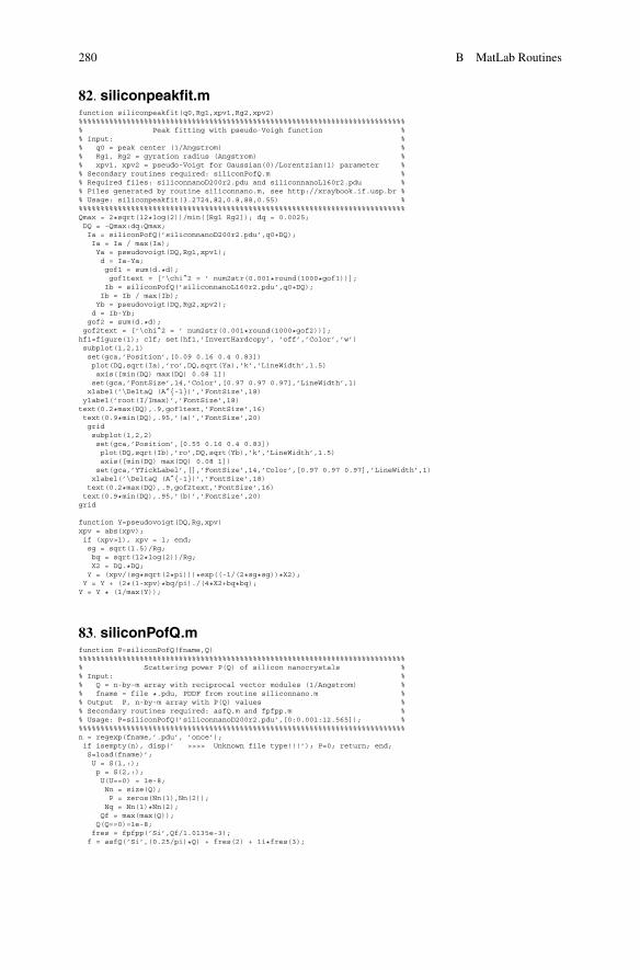
280 B MatLab Routines
82. siliconpeakfit.mfunction siliconpeakfit(q0,Rg1,xpv1,Rg2,xpv2)%%%%%%%%%%%%%%%%%%%%%%%%%%%%%%%%%%%%%%%%%%%%%%%%%%%%%%%%%%%%%%%%%%%%%%%%%%%% Peak fitting with pseudo-Voigh function %% Input: %% q0 = peak center (1/Angstrom) %% Rg1, Rg2 = gyration radius (Angstrom) %% xpv1, xpv2 = pseudo-Voigt for Gaussian(0)/Lorentzian(1) parameter %% Secondary routines required: siliconPofQ.m %% Required files: siliconnanoD200r2.pdu and siliconnanoL160r2.pdu %% Files generated by routine siliconnano.m, see http://xraybook.if.usp.br %% Usage: siliconpeakfit(3.2724,82,0.8,88,0.55) %%%%%%%%%%%%%%%%%%%%%%%%%%%%%%%%%%%%%%%%%%%%%%%%%%%%%%%%%%%%%%%%%%%%%%%%%%%%Qmax = 2*sqrt(12*log(2))/min([Rg1 Rg2]); dq = 0.0025;DQ = -Qmax:dq:Qmax;Ia = siliconPofQ(’siliconnanoD200r2.pdu’,q0+DQ);Ia = Ia / max(Ia);Ya = pseudovoigt(DQ,Rg1,xpv1);d = Ia-Ya;gof1 = sum(d.*d);gof1text = [’\chi^2 = ’ num2str(0.001*round(1000*gof1))];
Ib = siliconPofQ(’siliconnanoL160r2.pdu’,q0+DQ);Ib = Ib / max(Ib);Yb = pseudovoigt(DQ,Rg2,xpv2);d = Ib-Yb;
gof2 = sum(d.*d);gof2text = [’\chi^2 = ’ num2str(0.001*round(1000*gof2))];
hf1=figure(1); clf; set(hf1,’InvertHardcopy’, ’off’,’Color’,’w’)subplot(1,2,1)set(gca,’Position’,[0.09 0.16 0.4 0.83])plot(DQ,sqrt(Ia),’ro’,DQ,sqrt(Ya),’k’,’LineWidth’,1.5)axis([min(DQ) max(DQ) 0.08 1])set(gca,’FontSize’,14,’Color’,[0.97 0.97 0.97],’LineWidth’,1)
xlabel(’\DeltaQ (A^{-1})’,’FontSize’,18)ylabel(’root(I/Imax)’,’FontSize’,18)text(0.2*max(DQ),.9,gof1text,’FontSize’,16)text(0.9*min(DQ),.95,’(a)’,’FontSize’,20)gridsubplot(1,2,2)set(gca,’Position’,[0.55 0.16 0.4 0.83])plot(DQ,sqrt(Ib),’ro’,DQ,sqrt(Yb),’k’,’LineWidth’,1.5)axis([min(DQ) max(DQ) 0.08 1])set(gca,’YTickLabel’,[],’FontSize’,14,’Color’,[0.97 0.97 0.97],’LineWidth’,1)xlabel(’\DeltaQ (A^{-1})’,’FontSize’,18)
text(0.2*max(DQ),.9,gof2text,’FontSize’,16)text(0.9*min(DQ),.95,’(b)’,’FontSize’,20)grid
function Y=pseudovoigt(DQ,Rg,xpv)xpv = abs(xpv);if (xpv>1), xpv = 1; end;sg = sqrt(1.5)/Rg;bq = sqrt(12*log(2))/Rg;X2 = DQ.*DQ;
Y = (xpv/(sg*sqrt(2*pi)))*exp((-1/(2*sg*sg))*X2);Y = Y + (2*(1-xpv)*bq/pi)./(4*X2+bq*bq);
Y = Y * (1/max(Y));
83. siliconPofQ.mfunction P=siliconPofQ(fname,Q)%%%%%%%%%%%%%%%%%%%%%%%%%%%%%%%%%%%%%%%%%%%%%%%%%%%%%%%%%%%%%%%%%%%%%%%%%%%% Scattering power P(Q) of silicon nanocrystals %% Input: %% Q = n-by-m array with reciprocal vector modules (1/Angstrom) %% fname = file *.pdu, PDDF from routine siliconnano.m %% Output P, n-by-m array with P(Q) values %% Secondary routines required: asfQ.m and fpfpp.m %% Usage: P=siliconPofQ(’siliconnanoD200r2.pdu’,[0:0.001:12.565]); %%%%%%%%%%%%%%%%%%%%%%%%%%%%%%%%%%%%%%%%%%%%%%%%%%%%%%%%%%%%%%%%%%%%%%%%%%%%n = regexp(fname,’.pdu’, ’once’);if isempty(n), disp(’ >>>> Unknown file type!!!’); P=0; return; end;S=load(fname)’;U = S(1,:);p = S(2,:);U(U==0) = 1e-8;Nn = size(Q);P = zeros(Nn(1),Nn(2));Nq = Nn(1)*Nn(2);Qf = max(max(Q));Q(Q==0)=1e-8;fres = fpfpp(’Si’,Qf/1.0135e-3);
f = asfQ(’Si’,(0.25/pi)*Q) + fres(2) + 1i*fres(3);
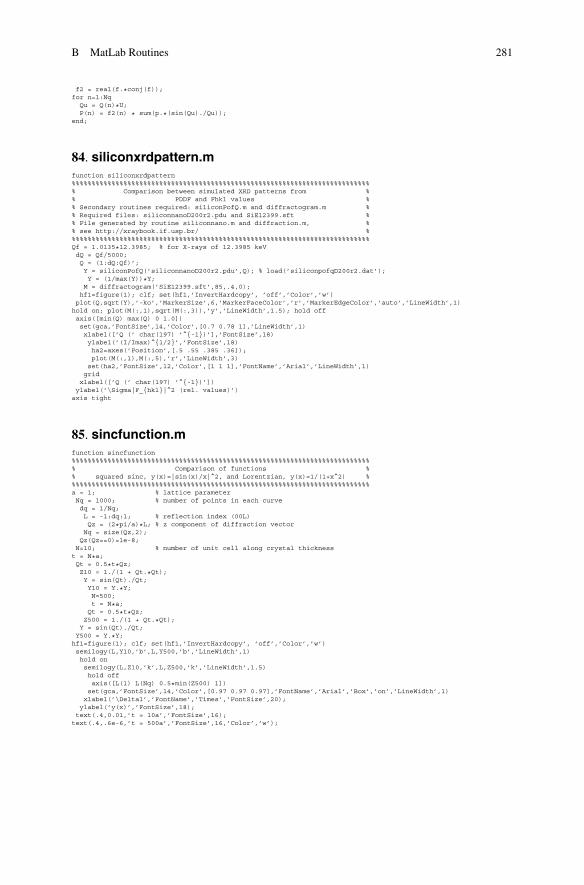
B MatLab Routines 281
f2 = real(f.*conj(f));for n=1:NqQu = Q(n)*U;P(n) = f2(n) * sum(p.*(sin(Qu)./Qu));
end;
84. siliconxrdpattern.mfunction siliconxrdpattern%%%%%%%%%%%%%%%%%%%%%%%%%%%%%%%%%%%%%%%%%%%%%%%%%%%%%%%%%%%%%%%%%%%%%%%%%%%% Comparison between simulated XRD patterns from %% PDDF and Fhkl values %% Secondary routines required: siliconPofQ.m and diffractogram.m %% Required files: siliconnanoD200r2.pdu and SiE12399.sft %% File generated by routine siliconnano.m and diffraction.m, %% see http://xraybook.if.usp.br/ %%%%%%%%%%%%%%%%%%%%%%%%%%%%%%%%%%%%%%%%%%%%%%%%%%%%%%%%%%%%%%%%%%%%%%%%%%%%Qf = 1.0135*12.3985; % for X-rays of 12.3985 keVdQ = Qf/5000;Q = (1:dQ:Qf)’;Y = siliconPofQ(’siliconnanoD200r2.pdu’,Q); % load(’siliconpofqD200r2.dat’);Y = (1/max(Y))*Y;M = diffractogram(’SiE12399.sft’,85,.4,0);
hf1=figure(1); clf; set(hf1,’InvertHardcopy’, ’off’,’Color’,’w’)plot(Q,sqrt(Y),’-ko’,’MarkerSize’,6,’MarkerFaceColor’,’r’,’MarkerEdgeColor’,’auto’,’LineWidth’,1)hold on; plot(M(:,1),sqrt(M(:,3)),’y’,’LineWidth’,1.5); hold offaxis([min(Q) max(Q) 0 1.0])set(gca,’FontSize’,14,’Color’,[0.7 0.78 1],’LineWidth’,1)xlabel([’Q (’ char(197) ’^{-1})’],’FontSize’,18)ylabel(’(I/Imax)^{1/2}’,’FontSize’,18)ha2=axes(’Position’,[.5 .55 .385 .36]);plot(M(:,1),M(:,5),’r’,’LineWidth’,3)set(ha2,’FontSize’,12,’Color’,[1 1 1],’FontName’,’Arial’,’LineWidth’,1)grid
xlabel([’Q (’ char(197) ’^{-1})’])ylabel(’\Sigma|F_{hkl}|^2 (rel. values)’)axis tight
85. sincfunction.mfunction sincfunction%%%%%%%%%%%%%%%%%%%%%%%%%%%%%%%%%%%%%%%%%%%%%%%%%%%%%%%%%%%%%%%%%%%%%%%%%%%% Comparison of functions %% squared sinc, y(x)=|sin(x)/x|^2, and Lorentzian, y(x)=1/(1+x^2) %%%%%%%%%%%%%%%%%%%%%%%%%%%%%%%%%%%%%%%%%%%%%%%%%%%%%%%%%%%%%%%%%%%%%%%%%%%%a = 1; % lattice parameterNq = 1000; % number of points in each curvedq = 1/Nq;L = -1:dq:1; % reflection index (00L)Qz = (2*pi/a)*L; % z component of diffraction vectorNq = size(Qz,2);
Qz(Qz==0)=1e-8;N=10; % number of unit cell along crystal thicknesst = N*a;Qt = 0.5*t*Qz;Z10 = 1./(1 + Qt.*Qt);Y = sin(Qt)./Qt;Y10 = Y.*Y;N=500;t = N*a;Qt = 0.5*t*Qz;Z500 = 1./(1 + Qt.*Qt);
Y = sin(Qt)./Qt;Y500 = Y.*Y;hf1=figure(1); clf; set(hf1,’InvertHardcopy’, ’off’,’Color’,’w’)semilogy(L,Y10,’b’,L,Y500,’b’,’LineWidth’,1)hold onsemilogy(L,Z10,’k’,L,Z500,’k’,’LineWidth’,1.5)hold offaxis([L(1) L(Nq) 0.5*min(Z500) 1])set(gca,’FontSize’,14,’Color’,[0.97 0.97 0.97],’FontName’,’Arial’,’Box’,’on’,’LineWidth’,1)xlabel(’\Deltal’,’FontName’,’Times’,’FontSize’,20);
ylabel(’y(x)’,’FontSize’,18);text(.4,0.01,’t = 10a’,’FontSize’,16);text(.4,.6e-6,’t = 500a’,’FontSize’,16,’Color’,’w’);
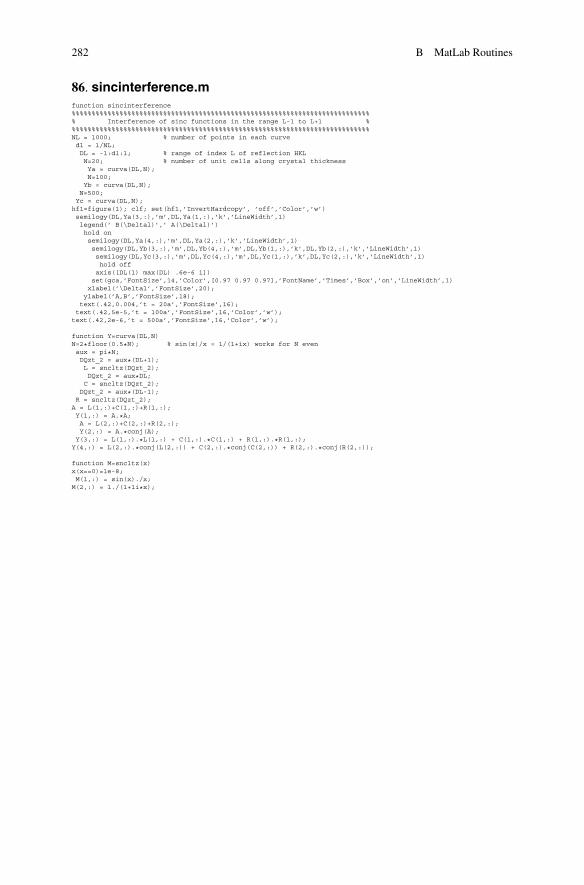
282 B MatLab Routines
86. sincinterference.mfunction sincinterference%%%%%%%%%%%%%%%%%%%%%%%%%%%%%%%%%%%%%%%%%%%%%%%%%%%%%%%%%%%%%%%%%%%%%%%%%%%% Interference of sinc functions in the range L-1 to L+1 %%%%%%%%%%%%%%%%%%%%%%%%%%%%%%%%%%%%%%%%%%%%%%%%%%%%%%%%%%%%%%%%%%%%%%%%%%%%NL = 1000; % number of points in each curvedl = 1/NL;DL = -1:dl:1; % range of index L of reflection HKLN=20; % number of unit cells along crystal thicknessYa = curva(DL,N);N=100;Yb = curva(DL,N);
N=500;Yc = curva(DL,N);hf1=figure(1); clf; set(hf1,’InvertHardcopy’, ’off’,’Color’,’w’)semilogy(DL,Ya(3,:),’m’,DL,Ya(1,:),’k’,’LineWidth’,1)legend(’ B(\Deltal)’,’ A(\Deltal)’)hold onsemilogy(DL,Ya(4,:),’m’,DL,Ya(2,:),’k’,’LineWidth’,1)semilogy(DL,Yb(3,:),’m’,DL,Yb(4,:),’m’,DL,Yb(1,:),’k’,DL,Yb(2,:),’k’,’LineWidth’,1)semilogy(DL,Yc(3,:),’m’,DL,Yc(4,:),’m’,DL,Yc(1,:),’k’,DL,Yc(2,:),’k’,’LineWidth’,1)hold offaxis([DL(1) max(DL) .6e-6 1])set(gca,’FontSize’,14,’Color’,[0.97 0.97 0.97],’FontName’,’Times’,’Box’,’on’,’LineWidth’,1)xlabel(’\Deltal’,’FontSize’,20);ylabel(’A,B’,’FontSize’,18);
text(.42,0.004,’t = 20a’,’FontSize’,16);text(.42,5e-5,’t = 100a’,’FontSize’,16,’Color’,’w’);text(.42,2e-6,’t = 500a’,’FontSize’,16,’Color’,’w’);
function Y=curva(DL,N)N=2*floor(0.5*N); % sin(x)/x = 1/(1+ix) works for N evenaux = pi*N;DQzt_2 = aux*(DL+1);L = sncltz(DQzt_2);DQzt_2 = aux*DL;C = sncltz(DQzt_2);
DQzt_2 = aux*(DL-1);R = sncltz(DQzt_2);A = L(1,:)+C(1,:)+R(1,:);Y(1,:) = A.*A;A = L(2,:)+C(2,:)+R(2,:);Y(2,:) = A.*conj(A);Y(3,:) = L(1,:).*L(1,:) + C(1,:).*C(1,:) + R(1,:).*R(1,:);Y(4,:) = L(2,:).*conj(L(2,:)) + C(2,:).*conj(C(2,:)) + R(2,:).*conj(R(2,:));
function M=sncltz(x)x(x==0)=1e-8;M(1,:) = sin(x)./x;M(2,:) = 1./(1+1i*x);
Bibliography
Als-Nielsen, J., McMorrow, D.: Elements of Modern X-Ray Physics. Wiley, New York (2001)Antunes, A., Safatle, A.M.V., Barros, P.S.M., Morelhão, S.L.: X-ray imaging in advanced studies
of ophthalmic diseases. Med. Phys. 33, 2338–2343 (2006). doi:10.1118/1.2207135Arfken, G.: Mathematical Methods for Physicists. Academic, Orlando (1985)Authier, A.:Dynamical Theory of X-Ray Diffraction, revised edn. Oxford University, Oxford
(2004)Authier, A. (ed.): International Tables for Crystallography, vol. D, online edition (2006). http://
onlinelibrary.wiley.com/book/10.1107/97809553602060000001/tocBarbosa, L.R.S.: Small angle X-ray scattering study of biological relevant systems. Ph.D. Thesis,
Institute of Physics, University of São Paulo (2008). http://www.teses.usp.br/teses/disponiveis/43/43134/tde-20032009-101046/pt-br.php
Batterman, B.W., Cole, H.: Dynamical diffraction of X-rays by perfect crystals. Rev. Mod. Phys.36, 681–717 (1964)
Bowen, D.K., Tanner, B.K.: High Resolution X-Ray Diffractometry and Topography. Taylor &Francis, London (1998)
Bragg, W.H., Bragg, W.L.: The reflexion of X-rays by crystals. Proc. R. Soc. Lond. A88, 428–438 (1913). doi: 10.1098/rspa.1913.0040. www.nobelprize.org/nobel_prizes/physics/laureates/1915/
Cattani, M.S.D.: X-R ay Scattering by Atoms: Basic Equations. Institute of Physics, University ofSão Paulo, São Carlos (2011). http://publica-sbi.if.usp.br/PDFs/pd1668.pdf
Chang, S.-L.: Multiple Diffraction of X-Rays in Crystals. Springer, Berlin (1984)Cohen-Tannoudji, C., Diu, B., Laloë, F.: Quantum Mechanics, vol. 2. Wiley, New York (1978)Coppens, P.: International Tables for Crystallography, vol. B, online edition, cap. 1.2, pp. 10–23
(2010). http://onlinelibrary.wiley.com/book/10.1107/97809553602060000001/tocCraievich, A.: Small-angle X-ray scattering by nanostructured materiais. In: Sakka, S. (ed.)
Handbook of Sol-Gel Science and Technology: Processing, Characterization and Applications,vol. II, pp. 161–189. Kluwer Academic, New York (2002)
Cullity, B.D., Stock, S.R.: Elements of X-Ray Diffraction, 3rd edn. Prentice-Hall, Upper SaddleRiver (2001)
Egami, T., Billinge, S.J.L. (eds.): Underneath the Bragg Peaks. Pergamon, Oxford (2003)Chapman, H.N., et al.: Femtosecond x-ray protein nanocrystallography. Nature 470, 73–77 (2011)Ewald, P.P.: Introduction to the dynamical theory of X-ray diffraction. Acta Crystallogr. A 25,
103–108 (1969)Franklin, R.E., Gosling, R.G.: Molecular configuration in sodium thymonucleate. Nature 171,
740–741 (1953). doi:10.1038/171740a0
© Springer International Publishing Switzerland 2016S.L. Morelhão, Computer Simulation Tools for X-ray Analysis,Graduate Texts in Physics, DOI 10.1007/978-3-319-19554-4
283
284 Bibliography
Giacovazzo, C. (ed.): Fundamentals of Crystallography, 2nd edn. Oxford University, Oxford (2002)Glatter, O., Kratky, O. (eds.): Small Angle Scattering of X-Rays. Academic, London (1982)Guinier, A.: X-ray Diffraction: In Crystals, Imperfect Crystals, and Amorphous Bodies. Dover,
New York (1994)Guinier, A., Fournet, G.: Small-Angle Scattering of X-Rays. Wiley, New York (1955)Hahn, T. (ed.): International Tables for Crystallography, vol. A, online edition (2006). http://
onlinelibrary.wiley.com/book/10.1107/97809553602060000001/tocHansen, J.-P., McDonald, I.R.: Theory of Simple Liquids, 2nd edn. Academic, London (1990)Hauptman, H.A., Karle, J.: Solution of the phase problem I. The centrosymmetric crystal. A.C.A.
Monograph No.3. Polycrystal Book Service, New York (1953). http://www.nobelprize.org/nobel_prizes/chemistry/laureates/1985/
Holt, M., Wu, Z., Hong, H., Zschack, P., Jemian, P., Tischler, J., Chen, H., Chiang, T.-C.:Determination of phonon dispersions from x-ray transmission scattering: the example ofsilicon. Phys. Rev. Lett. 83, 3317–3319 (1999)
Hubbell, J.H., Veigele, W.J., Briggs, E.A., Brown, R.T., Cromer, D.T., Howerton, R.J.: Atomicform factors, incoherent scattering functions, and photon scattering cross sections. J. Phys.Chem. Ref. Data 4, 471–538 (1975)
Hura, G., Russo, D., Glaeser, R.M., Head-Gordon, T., Krack, M., Parrinello, M.: Water structure asa function of temperature from x-ray scattering experiments and ab initio molecular dynamics.Phys. Chem. Chem. Phys. 5, 1981–1991 (2003)
James, R.W.: The Optical Principles of the Diffraction of X-rays, 1st edn. G. Bell & Sons Ltd,London (1948)
Lindner, P., Zemb, T. (eds.): Neutrons, X-Rays and Light: Scattering Methods Applied to SoftCondensed Matter. Elsevier, Amsterdam (2002)
Lovesey, S.W., Collins, S.P.: X-Ray Scattering and Absorption by Magnetic Materials. OxfordUniversity, Oxford (1996)
Malachias, A., Freitas, R., Morelhão, S.L., Magalhães Paniago, R., Kycia, S., Medeiros-Ribeiro,G.: X-ray diffraction methods for studying strain and composition in epitaxial nanostructuredsystems. In: Haight, R., Ross, F.M., Hannon, J.B. (eds.) Handbook of Instrumentation andTechniques for Semiconductor Nanostructure Characterization, vol. 1, pp. 211–279. WorldScientific, Washington, D.C. (2011). doi:10.1142/9789814322843_0006
Morelhão, S.L., Amirkhanyan, Z.G., Rémedios, C.M.R.:Absolute refinement of crystal structuresby X-ray phase measurements. Acta Crystallogr. A 71 (2015). doi:10.1038/171740a0
Morelhão, S.L., Brito, G.E.S., Abramof, E.: Nanostructure of sol.gel films by X-ray specularreflectivity. Appl. Phys. Lett. 80, 407–409 (2002). doi:10.1063/1.1436271
Morelhão, S.L., Härtwig, J., Meier, D.L.:Dislocations in dendritic web silicon. J. Cryst. Growth213, 288–298 (2000)
Morelhão, S.L., Remédios, C.M.R., Freitas, R.O., dos Santos, A.O.: X-ray phase measurements asa probe of small structural changes in doped nonlinear optical crystals. J. Appl. Crystallogr. 44,93–101 (2011)
Stöhr, J.: Nexasf Spectroscopy. Springer, Berlin (1992)McMaster, W.H., Grande, N.K.D., Mallett, J.H., Hubbell, J.H.: Compilation of X-ray cross
sections. Lawrence Livermore National Laboratory Report UCRL-50174 Section II Revision I(1969). Available from National Technical Information Services L-3, U.S. Dept. of Commerce.http://cars9.uchicago.edu/~newville/mcbook/
Newville, M.: The Fundamentals of XASF, Chicago (2004). http://xafs.org/TutorialsPietsch, U., Holý, V., Baumbach, T.: High-Resolution X-Ray Scattering: From Thin Films to
Lateral Nanostructures, 2nd edn. Springer, New York (2004)Pirenne, M.H.: The Diffraction of X-Rays and Electrons by Free Molecules. Cambridge University,
Cambridge (1946)Prince, E. (ed.): International Tables for Crystallography, vol. C, online edition (2006). http://
onlinelibrary.wiley.com/book/10.1107/97809553602060000001/tocTeixeira, J.: Small-angle scattering by fractal systems. J. Appl. Crystallogr. 21, 781–785 (1988)

Bibliography 285
Vocadlo, D.J., Davies, G.J., Laine, R., Withers, S.G.: Catalysis by hen egg-white lysozymeproceeds via a covalent intermediate. Nature 412, 835–838 (2001)
von Laue, M.: Eine quantitative prufung der theorie fur die interferenzerscheinungen bei ront-genstrahlen. Ann. Phys. 346, 989–1002 (1913). doi:10.1002/andp.19133461005. http://www.nobelprize.org/nobel_prizes/physics/laureates/1914/
Vuolo, J.H.: Fundamentos da Teoria de Erros, 2a: edn. Edgard Blucher, São Paulo (1996)Warren, B.E.: X-Ray Diffraction. Dover Books on Physics, New York (1990).Watson, J.D., Crick, F.H.C.: A structure for deoxyribose nucleic acid. Nature 171, 737–738 (1953).
doi:10.1038/171737a0. www.nobelprize.org/nobel_prizes/medicine/laureates/1962/Weckert, E., Hümmer, K.: Multiple-beam X-ray diffraction for physical determination of reflection
phases and its applications. Acta Crystallogr. A 53, 108–143 (1997)Wilkins, M.H.F., Stokes, A.R., Wilson, H.R.: Molecular structure of deoxypentose nucleic acids.
Nature 171, 738–740 (1953). doi:10.1038/171738a0Yi, Z., Ye, J., Kikugawa, N., Kako, T., Ouyang, S., Stuart-Williams, H., Yang, H., Cao, J., Luo, W.,
Li, Z., Liu, Y., Withers, R.L.: An orthophosphate semiconductor with photooxidation propertiesunder visible-light irradiation. Nat. Mater. 9, 559–564 (2010)
Zachariasen, W.H.: Theory of X-Ray Diffraction in Crystals. Wiley, New York (1945)
Index
AAbsorption, X-ray, 1. See also Photoelectric
absorptionatomic resonance, 42–45
semi-classical approach of, 45–48cross-section, 39–41, 43–47
for Kr, 48modulation in, 53–54
Kramers–Kronig relations, 48–50linear attenuation coefficient, 39–42
and scattering cross-section, 40–42modulation by rescattering of
photoelectrons, 50–56Absorption edge measurement, 206–209
experimental data, 207photoelectric absorption cross-section,
208–209transmission coefficients, 208
˛�quartzatomic structure, 120–121
RDF of, 121critical angle of, 192–193disordering periodic structures, 121–123
Alumina, XRD analysis of. See X-raydiffraction (XRD) analysis ofalumina
Amorphous solids, 116coordination number, RDF, 117correlation function, 118crystallization (see Crystallization)effect of interference in, 40periodic structures, disordering, 121
Amplituderesonance, 42, 44–47, 148
modulation, 56
scattering, 212of atoms, 23, 26, 28and polarization, 3and radiation field, 5–6
structure factor, 135–137, 160, 165Anomalous scattering factors. See Dispersion
correction termsArbitrary correlations
amorphous solid, 116coordination number, RDF, 117correlation function, 118crystallization (see Crystallization)periodic structures, disordering, 121
liquids and colloidal suspensionsRDF, 109in water, 109–111
mutual interference, 102non-spherical particles, 100–101radial distribution function
intensity scattered, 116N particles distribution, 111numerical calculation, 112packing factor, 116random positions, generation, 112–113repulsion effect, 113–115
volume effectsdeduction, functions, 105–106Fourier transform, 103interference function calculation, 108scattered intensity, 107unidirectional correlation, function,
104asfQ.m routine, 24, 110, 203, 213–214assintotic.m routine, 214Asymptotic behavior, 72, 73, 75, 97–99
© Springer International Publishing Switzerland 2016S.L. Morelhão, Computer Simulation Tools for X-ray Analysis,Graduate Texts in Physics, DOI 10.1007/978-3-319-19554-4
287
288 Index
Atomic form factor. See Atomic scatteringfactor
Atomic planescoherent scattering by, 132X-ray wavefronts crossing, 190
Atomic resonance, 42–45absorption cross-section for Kr, 48and refraction index, 192semi-classical approach of, 45–48
Atomic scattering factor, 23–24, 26–27,42
coherent scattering cross-section forSe, 44–45
with dispersed correction, 43for Ga, 26, 27
AtomsCompton scattering by, 33–36isolated, coherent scattering cross-section
for, 27–28spherosymmetrical, 23–27
Attenuation coefficient. See Linear attenuationcoefficient
Bbackadj.m routine, 203, 214Benzene molecule, scattering by, 32–33benzeneonpsp.m routine, 32, 214–215benzenesaxs1.m routine, 215–217benzenesaxs2.m routine, 217Biot–Savart law, 2Bragg–Brentano geometry, 164bragg.m routine, 133, 158, 217–218Bragg’s angle, 155, 182, 183Bragg’s law, 132, 133, 144, 182Bremsstrahlung. See Lae method
CCalcium, Compton scattering cross-section
for, 35Carbon, coherent/incoherent intensities
scattered by, 36Cauchy’s integral theorem, 49CIF. See Crystallographic information file
(CIF)Classical electron radius, 6Coherence lengths, 8–11Coherent scattering, 2, 12
by atomic planes, 132of atoms, 23–24cross-section
effect of atomic resonance in, 44–45for isolated atoms, 27–28
interference phenomena of, 40of one electron, 19–21
Complex systemsarbitrary correlations (see Arbitrary
correlations)internal correlations (see Internal
correlations)mathematical description of, 81
Compton effect, 1–2, 20, 33–35, 41Compton scattering, 1–2, 19–22, 64–66, 89,
119, 209by atoms, 33–36intensity, 20–21
Convolution of functions, 16Correlation function, 82–83, 93, 102, 104–105,
107, 117–118, 143internal, 84–85, 101pair (see Radial distribution function
(RDF))Critical angle for total external reflection, 191
in glass surfaces, 192Cromer–Mann coefficients, 24–25Cross-section
absorption, 39–41, 43–47for Kr, 48modulation in, 53–54
coherent scatteringeffect of atomic resonance, 44–45for isolated atoms, 27–28monoatomic gas, 60, 61parametric equation, 27for Se, 45
Compton scattering, 35parametric equation, 34
linear attenuation, 40–42photoelectric absorption, 50–52
for absorption edge measurement,208–209
Thomson scattering, 6–7Crystalline lattice
atomic disordering inoccupancy factor, 147–148thermal vibrations, 142–144
FT of, 130phonons, 144thermal diffuse scattering, 144truncation of, 138–139
Crystallization, of amorphous solids, 119˛�quartz, 120–122inverse FT, 122structural analysis, 123–124
Index 289
Crystallographic information file (CIF), 158XRD pattern simulation from, 204–205
Crystallography. See X-ray crystallographyCrystals
atomic disorderingoccupancy factor, 147–148thermal vibrations, 142–144
coherent intensity, 131crystalline lattice, 129diffracted intensities, 131, 134–135electron density, 129form factor, 130, 134, 144FT of crystalline lattice, 130kinematic intensity, 138, 143reciprocal lattice point, 131, 132, 134reciprocal lattice vector, 131, 133, 134,
153, 154, 158, 159reciprocal space of, 135reflectivity curves in, 182–185structure factors, 134
amplitude, 135, 137phases (direct methods), 137
truncation of crystal lattice, 138–139unit cell, 128X-ray diffraction, difficulties, 127–128
csfQ.m routine, 34, 218–219
DDarwin–Prins dynamical theory, 179, 181Data analysis
absorption edge, measurement of, 206–209PDDF analysis of lysozyme, 195–197PDF analysis of gold particles, 197–201XRD analysis of alumina, 201–206
debye.m routine, 94, 219Debye–Waller factor, 93–94, 97, 144, 162, 206Diffracted intensity, 131, 134Diffraction imaging techniques, 179–180diffraction.m routine, 146, 158, 203, 220–221Diffraction pattern
crystallized insulin, 174polychromatic, spodumene crystal, 173of polycrystalline silicon, 162
Diffractogram, polycrystalline silicon, 161,163
diffractogram.m routine, 203, 206, 222Diffractometry. See Single crystal
diffractometryDirac delta function, 15Dispersion correction terms, 44Dynamical diffraction
kinematic limit, 187–190recursive equations, 180–187
reflection/transmission coefficients bycrystallographic planes, 181–182
refraction index for X-rays, 190–193dynamicphase.m routine, 186, 223
EElastically bound electron, 45–48Elastic scattering. See Thomson scatteringElectric dipole radiation, 2
by free electron, 211–212Electron density
of atoms, 23crystals, 129of molecules, 28–29with radial symmetry, form factor for, 17small angle scattering, 69–70spherical particles, 85–86uniform spherical, relative intensity
scattered by, 18volumetric electron density function, 13
Ewald’s spheres. See Scattering spheresex1GUP.m routine, 115, 223ex1N5U.m routine, 70, 224exabscs.m routine, 224–225EXAFS. See Extended XAFS (EXAFS)exanomalousignal.m routine, 185, 225exasf.m routine, 26–27, 226excompton.m routine, 226–227excritangle.m routine, 192, 227excsf.m routine, 36, 227–228exellipsoid.m routine, 228exexafsmap.m routine, 230exexafs.m routine, 53, 229–230exfpfpp.m routine, 231exgofu1.m routine, 104, 232exgofu2.m routine, 108, 232–233exgoldnano0.m routine, 90, 233exgoldnano1.m routine, 92, 234exgoldnano2.m routine, 93, 234–235exhardsphere.m routine, 117, 235–236exkk.m routine, 236–237exlognormal.m routine, 78, 237–238exlysozyme.m routine, 88, 238–239exrdffitting.m routine, 113, 240exrdf.m routine, 239–240exrdfplot.m routine, 114, 240–241exrlp3Dview.m routine, 241exsgc.m routine, 242exsgr.m routine, 242–243exshell.m routine, 86, 243–244exsphere.m routine, 18, 245Extended XAFS (EXAFS), 54–55exwaterccd.m routine, 111, 245–246exwaterSofQ.m routine, 110, 246
290 Index
FFluorescence, 1, 38, 42–43, 53Form factor, 14, 16–17, 29
atomic (see Atomic scattering factor)crystals, 130, 134, 144molecular, 31, 63single electron scattering, 19for spherosymmetric electron density, 17for uniform sphere, 17
Fourier analysis, 54–55in PDF analysis of gold particles, 201
Fourier transform (FT), 15–18of convolution and product, 16of crystalline lattice, 130inverse, 15, 83, 85–87, 89, 109, 117, 119,
122, 196–197Four-reflection monochromator, 4–5fpfpp.m routine, 44, 164, 207, 246–247Free electrons
electric dipole radiation by, 211–212interaction, 1–11
coherence lengths, 8–11polarization effects, 2–5radiation field, 5–8
X-ray scattering by distribution of, 12–22distributions of one electron and
Compton scattering, 19–22Fourier transform, 15–18
Friedel’s pair, 184FT. See Fourier transform (FT)fthofu.m routine, 247–248fthofuplotmap.m routine, 103, 248–249fthofuR.m routine, 103, 249Full width at half maximum (FWHM),
160–162
GGaAs crystals, reflectivity curves for, 185Gallium, atomic scattering factor for, 26, 27Gases
ideal, effect of interference in, 40monoatomic (see Monoatomic gas)
goldnano.m routine, 249–250Gold nanoparticles
PDDFs, 93wide angle, 91–92X-ray scattering, 91–92
Gold particles, PDF analysis of. See Pairdensity function (PDF)
Goniometer, 165–166, 168
Grazing incidence techniques, 138, 155, 191Gyration radius, in PDDF analysis of
lysozyme, 197
Hhistogram.m routine, 250–251
IIdeal gas, effect of interference in, 40Incident wave, X-ray, 2Incoherent scattering. See Compton scatteringInelastic scattering. See Compton scatteringIntegrated intensity, 156, 160, 165, 167Integrated reflectivity of crystals, 187–188Intensity, scattering, 3–4, 6–7, 14. See also
Kinematic intensityarbitrary correlations, 107, 116coherent, 27, 28Compton scattering, 2, 20–21crystals
coherent intensity, 131kinematic intensity, 138, 143
relative intensity scattered by uniformspherical electron density, 18
single electron, 19by single molecule, 29–32
Interference, 12dispersed molecules, 64mutual interference, 81–82self-interference, 19–20
Internal correlationsmolecules, proteins, and discrete particles,
86–87limit of small angle, 87–89wide angle solution, 89–94
PDDF, 84random conformation particles
asymptotic behavior, 97–99polymers (see Polymers)
scattering power, 84spherical particles, radial electron density,
85–86spherosymmetrical function, 84
Interplanar distances, 132, 133, 157–158, 165Inverse Fourier transform, 15, 83, 85–87, 89,
109, 117, 119, 122, 196–197invftpofq.m routine, 251–252Ionization, effect on scattering amplitude, 26Iron, modulation of resonance amplitude of, 56Isotropic vibrations, 142–143
Index 291
JJoule heating effect, 38
KKDP. See Potassium dihydrogen phosphate
(KDP)kdpcoordfrac.m routine, 202, 252kdphistcomp.m routine, 252–253kdphistogram.m routine, 253Kinematic diffraction
vs. dynamical diffraction, 179–180powder diffractometry
crystallographic information file,158
polycrystalline samples, relativeintensities, 158–161
protein crystals, 174–176reciprocal space
coherent radiation, 152Ewald’s spheres (see Scattering spheres)scattering spheres, 152
reflection/transmission coefficients,182
single crystal diffractometrymonochromatic radiation, 165–167polychromatic radiation, 170–171
validity, 189–190Kinematic intensity, 59
dispersed moleculescoherent intensity scattered by N
molecules, 63interference pattern, 64molecule form factor, 63scattered intensity by single molecule,
63scattering power, 64structural function, 64
general expression of, 59monoatomic gas
beam transverse coherence length, 61coherent scattering cross-section, 60,
61Fourier transform, 60
small angle scatteringdispersion of size, 74–78macromolecules, 68–69morphology of particles, 71–74particles of uniform density, 69–70polydisperse systems, 74–78
Kinematic limit, 187–190kinematiclimit.m routine, 188, 190, 253–254Kramers–Kronig relations, 43, 48–50, 55Krypton, absorption cross-section for, 48
LLaue method, 171lauemethod.m routine, 173, 254–256Linear attenuation, and scattering cross-
section, 40–42Linear attenuation coefficient, 39–42Longitudinal coherence length, 9–11Lorentz factor, 156Lysozyme
integrated reflectivity in, 188interatomic distances, 88PDDF (see Pair distance distribution
function (PDDF), lysozymeanalysis)
scattering power, 88–89
MManganese, modulation in absorption
cross-section of, 53–54Maxwell’s equations, 5, 211Molecular form factor, 31Molecules
dispersedcoherent intensity scattered by N
molecules, 63form factor, 63interference pattern, 64scattered intensity by single molecule,
63scattering power, 64structural function, 64
scattering by, 28–33Monoatomic gas
beam transverse coherence length, 61coherent scattering cross-section, 60, 61Fourier transform, 60scattering angle, 60
Monochromatic radiationcharge coupled device, 166goniometer, 165, 168high structural complexity crystals, 166integrated intensity, 165low structural complexity crystals, 165reflection power (see Integrated intensity)rotating crystal method, 166, 167
Monocrystalline blocks with channel cut, 184Mutual interference, 81–82
NNear-edge X-ray absorption spectrum
(NEXAFS), 53Nodes. See Reciprocal lattice points (RLPs)
292 Index
Oorientcryst.m routine, 257–258Oxygen, coherent scattering cross-section for,
28
PPair correlation function. See Radial
distribution function (RDF)Pair density function (PDF), analysis of gold
particles, 197–201background correction, 199–200Fourier analysis, 201loading intensity data, 199normalizing S(Q), 200–201structural function S(Q), 199
Pair distance distribution function (PDDF), 84,161–163
lysozyme analysis, 195–197gyration radius, 197inverse Fourier transform, 196–197loading intensity data, 196
Parametric equation, 24of coherent scattering cross-section, 27of Compton scattering cross-section, 34
Patterson function, 82–83pdbcoordfrac.m routine, 175, 177, 258–259PDDF. See Pair distance distribution function
(PDDF)PDF. See Pair density function (PDF)Phase problem, 28–33Phonons, 144Photoelectric absorption, 40
and dynamical diffraction, 182, 183modulation by rescattering of, 50–56
cross-section of Mn, 52–53scattering properties by neighboring
atoms, 53and refraction index, 191
Photoelectrons, 38, 40, 42, 47wavevector with kinetic energy, 50–51
Photon–electron interaction, 19–20Photon energy, 1photonsonpsp.m routine, 259photonstatistic.m routine, 260Polarization coefficient, 22Polarization effects, on free electron radiation,
2–4electron in forced vibration, 3
Polychromatic radiation, 170–171Polycrystals, relative intensities in, 158–164polymerchain.m routine, 95, 260–261polymerkratky.m routine, 98, 261–262polymer.m routine, 260
polymerRg.m routine, 99, 262Polymers
plastic bags, 97–98RW model, 96scattering power, 94–95
polymersystem.m routine, 262Porod’s law, 76Potassium dihydrogen phosphate (KDP),
145–147Powder diffractometry of polycrystals
area profile of diffraction peaks, 160–161,163
geometric factors, 158–159line profile of diffraction peaks, 160–161,
163Probability density function, 19–21
QQuantum electrodynamics (QED), 19quartzgofu.m routine, 122, 263quartzIofQ.m routine, 122, 264quartzrdf.m routine, 266–267quartzrdfplot.m routine, 121, 267quartzR.m routine, 120, 121, 264–266
RRadial distribution function (RDF), 109
atomic structure of ˛-quartz, 121intensity scattered, 116N particles distribution, 111numerical calculation, 112packing factor, 116random positions, generation, 112–113repulsion effect, 113–115
Radiation–electron elementary interaction. SeeFree electron interaction
Radiation field, in free electron interaction,5–8, 14
Radius of gyration, 67, 75rcdarwinprins.m routine, 184, 189, 267–269rcdarwinprinsplot.m routine, 183, 269RDF. See Radial distribution function (RDF)Reciprocal lattice, crystals, 130, 131Reciprocal lattice points (RLPs), 131, 132,
134Reciprocal node, 154–156, 166, 170, 171Reciprocal space, 152–154, 159, 161, 171,
174Recursive equations, 180–187
standing waves, 186–187Reflected beam geometry. See Bragg–Brentano
geometry
Index 293
Reflection power. See Integrated intensityReflectivity curves, in crystals, 182–185
dynamic phase as function of, 186Refraction index for X-rays, 190–193
critical angle for total external reflection inglass surfaces, 192–193
wavefronts crossing atomic plane, 190Relative intensities in polycrystals, 158–164Resonance. See Atomic resonanceRLPs. See Reciprocal lattice points (RLPs)rockingcurve.m routine, 269–270Rocking curves, 155, 157, 160Root mean square deviation, atomic positions,
144, 146rotatcryst.m routine, 270–272Rotating crystal method, 166, 167, 174, 175rotcrystmethod.m routine, 175, 272–274
SSAXS. See Small angle X-ray scattering
(SAXS)saxs.c routine, 68, 70, 274saxs.m routine, 87, 275Scalar polarization factor, 4Scattering spheres, 152, 153, 159, 160Schrödinger equation, 51Selenium, coherent scattering cross-section for,
44–45Self-interference, 19–20sfactor.m routine, 158, 202, 275–276sgcompton.m routine, 34, 42, 164, 209,
276–277sgrayleigh.m routine, 27, 42, 164, 209,
277–278siliconDScamera.m routine, 278–279siliconnano.m routine, 161, 279siliconpeakfit.m routine, 280siliconPofQ.m routine, 161, 280–281siliconxrdpattern.m routine, 281sincfunction.m routine, 281sincinterference.m routine, 282Single crystal diffractometry
monochromatic radiationgoniometer, 165high structural complexity, 166low structural complexity, 165rotating crystal method, 166, 167
polychromatic radiation, 170–171Single electron scattering, 19–22
form factor, 19intensities, 19, 21
Small angle scatteringmacromolecules
pdb format, 68protein data bank, 68
morphology of particlesasymptotic behaviors, 72, 73exponential decay, 71Guinier region, 71, 72Porod region, 71, 72spherical particle, 71
particles of uniform densityelectron density, 69–70small angle X-ray scattering, 70
polydisperse systemsaverage gyration radius, 67, 75dispersion of size, 75intensity, 75Porod’s law, 76
property of, 67Small angle X-ray scattering (SAXS), 70Snell’s law, 191Solids. See Amorphous solidsSpherosymmetrical atoms, 23–27Spherosymmetric electron density, form factor
for, 17Standing waves methods, 179–180, 186–187Synchrotron, 3, 33, 41, 43, 54, 170, 191
TTDS. See Thermal diffuse scattering (TDS)Temperature factor. See Debye–Waller factorThermal diffuse scattering (TDS), 144Thickness of crystals
and integrated reflectivity, 187–188and reflection and transmission coefficients,
189Thomson scattering, 1–2, 6–7, 19
differential cross-section of, 6total cross-section of, 7by volumetric distribution of free
electrons, 13Thomson scattering length. See Classical
electron radiusTransverse coherence length, 9–10
VVectorial Bragg’s law, 153Vector polarization factor, 3, 212Volumetric electron density function, 13
WWavevectors, 152, 154, 167, 169, 170, 175
294 Index
XX-ray absorption fine structure (XAFS), 50X-ray absorption near-edge spectroscopy
(XANES), 53X-ray absorption spectroscopy, 40X-ray crystallography, 28–29. See also Crystals
crystalline lattice, 129crystal’s electron density, 129crystal’s form factor, 130diffracted intensities, 134–135FT of crystalline lattice, 130
structure factors, 134–135unit cell, 128
X-ray diffraction (XRD) analysis of alumina,201–206
background intensity, adjusting, 204comparison of experimental and simulated
patterns, 205–206loading intensity data, 203pattern simulation from CIF, 204–205
X-ray optics, 179, 184, 190X-ray specular reflectometry, 191