Appendix A. GIS-Based Soil Erosion and Sedimentation

Appendix A.

GIS-Based Soil Erosion and Sedimentation Analysis Report

HYDROLOGY AND WATER QUALITY SPECIALIST REPORT Appendix A. GIS‐Based Soil Erosion & Sedimentation Analysis Report

A‐1 December 2008

1. INTRODUCTION

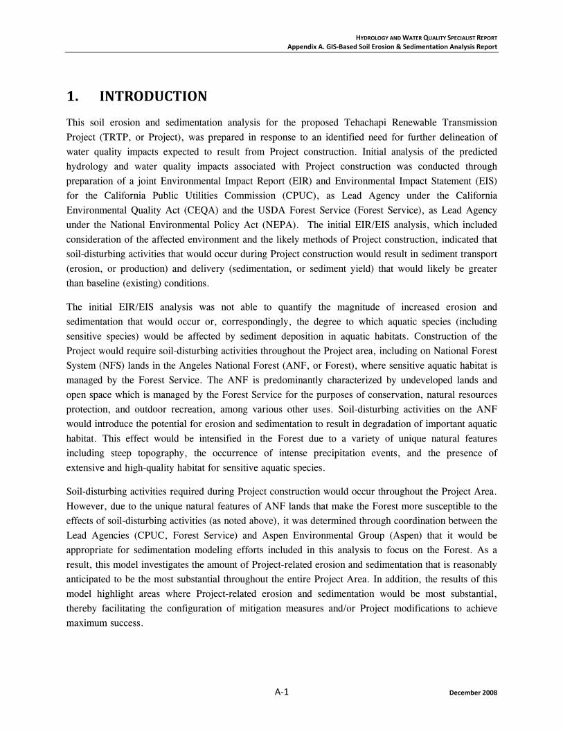
This soil erosion and sedimentation analysis for the proposed Tehachapi Renewable Transmission Project (TRTP, or Project), was prepared in response to an identified need for further delineation of water quality impacts expected to result from Project construction. Initial analysis of the predicted hydrology and water quality impacts associated with Project construction was conducted through preparation of a joint Environmental Impact Report (EIR) and Environmental Impact Statement (EIS) for the California Public Utilities Commission (CPUC), as Lead Agency under the California Environmental Quality Act (CEQA) and the USDA Forest Service (Forest Service), as Lead Agency under the National Environmental Policy Act (NEPA). The initial EIR/EIS analysis, which included consideration of the affected environment and the likely methods of Project construction, indicated that soil-disturbing activities that would occur during Project construction would result in sediment transport (erosion, or production) and delivery (sedimentation, or sediment yield) that would likely be greater than baseline (existing) conditions.

The initial EIR/EIS analysis was not able to quantify the magnitude of increased erosion and sedimentation that would occur or, correspondingly, the degree to which aquatic species (including sensitive species) would be affected by sediment deposition in aquatic habitats. Construction of the Project would require soil-disturbing activities throughout the Project area, including on National Forest System (NFS) lands in the Angeles National Forest (ANF, or Forest), where sensitive aquatic habitat is managed by the Forest Service. The ANF is predominantly characterized by undeveloped lands and open space which is managed by the Forest Service for the purposes of conservation, natural resources protection, and outdoor recreation, among various other uses. Soil-disturbing activities on the ANF would introduce the potential for erosion and sedimentation to result in degradation of important aquatic habitat. This effect would be intensified in the Forest due to a variety of unique natural features including steep topography, the occurrence of intense precipitation events, and the presence of extensive and high-quality habitat for sensitive aquatic species.

Soil-disturbing activities required during Project construction would occur throughout the Project Area. However, due to the unique natural features of ANF lands that make the Forest more susceptible to the effects of soil-disturbing activities (as noted above), it was determined through coordination between the Lead Agencies (CPUC, Forest Service) and Aspen Environmental Group (Aspen) that it would be appropriate for sedimentation modeling efforts included in this analysis to focus on the Forest. As a result, this model investigates the amount of Project-related erosion and sedimentation that is reasonably anticipated to be the most substantial throughout the entire Project Area. In addition, the results of this model highlight areas where Project-related erosion and sedimentation would be most substantial, thereby facilitating the configuration of mitigation measures and/or Project modifications to achieve maximum success.


December 2008 A‐2

As described in detail below (please see Section 3: Methodology), implementation of this model was based on the use of Geographic Information Systems (GIS) technology. This GIS-based approach enabled the quantification of erosion and sedimentation under both baseline and post-construction Project conditions. Quantification of the magnitude of increase erosion and sedimentation over baseline conditions subsequently facilitates analysis of the impacts of Project-related erosion and sedimentation on aquatic habitat and sensitive aquatic species. The data produced by this analysis are useful to identify areas of high erosion and sedimentation, as well as to compare Project alternatives, which also facilitates the Forest Service’s assessment of which Project alternative would be most consistent with federal management goals in the Project Area.

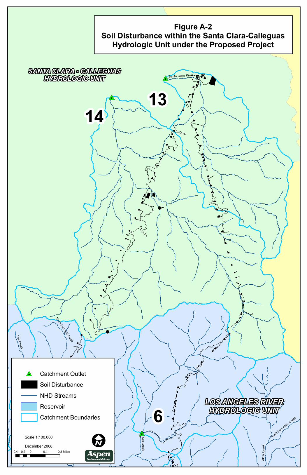
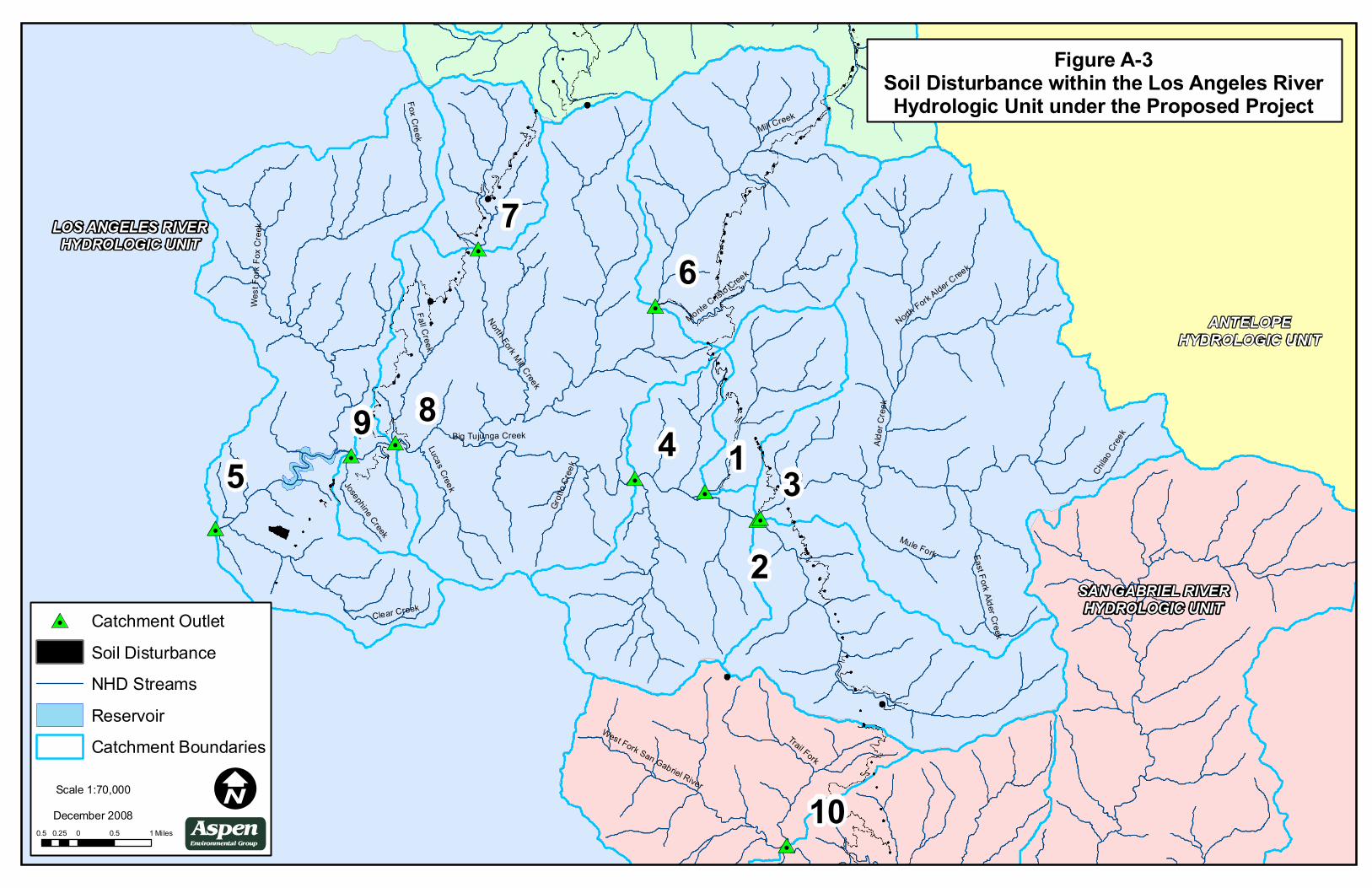
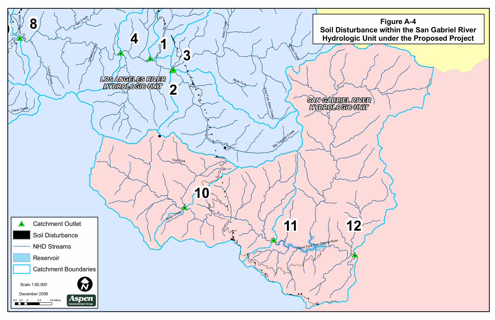
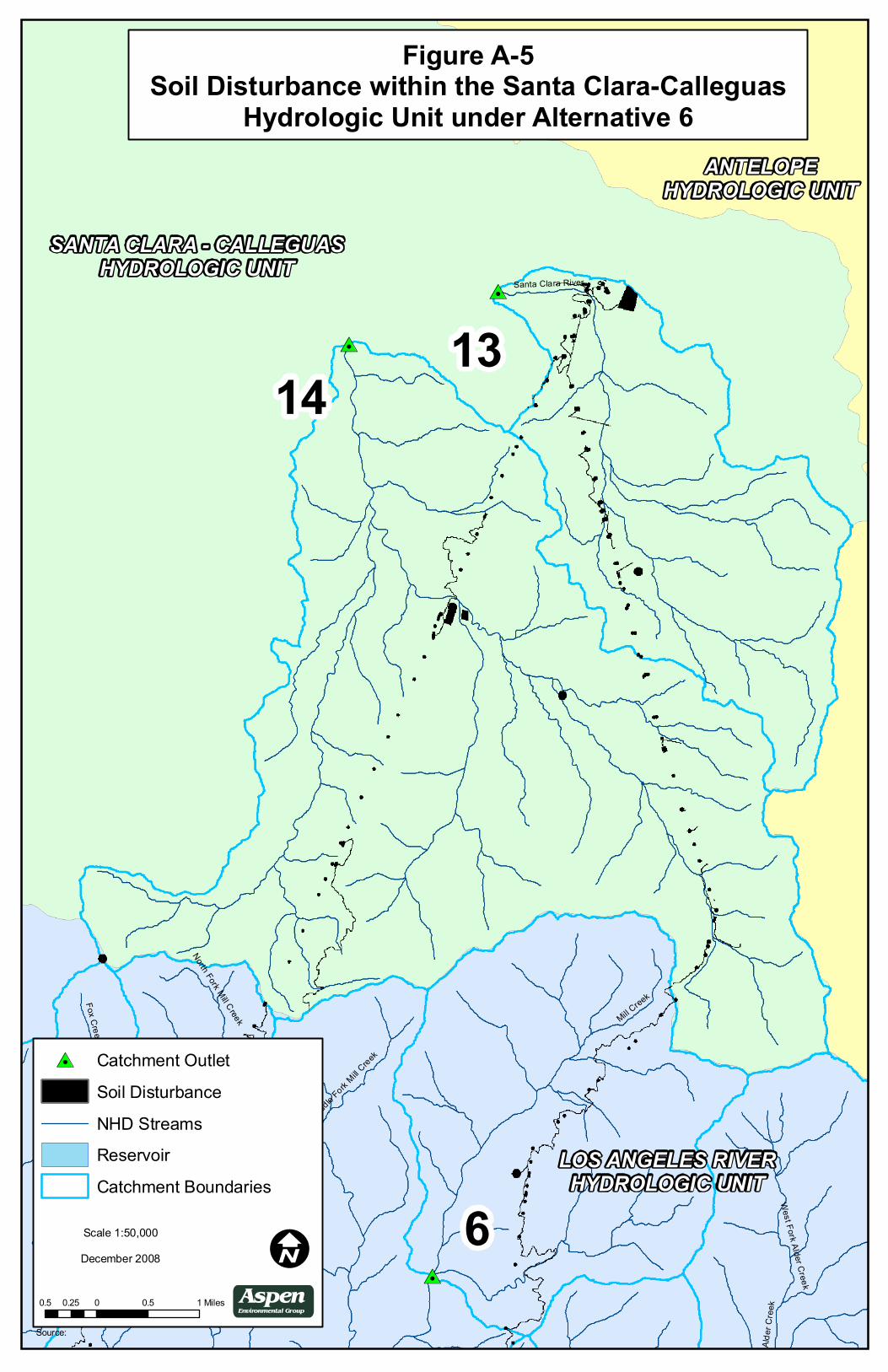
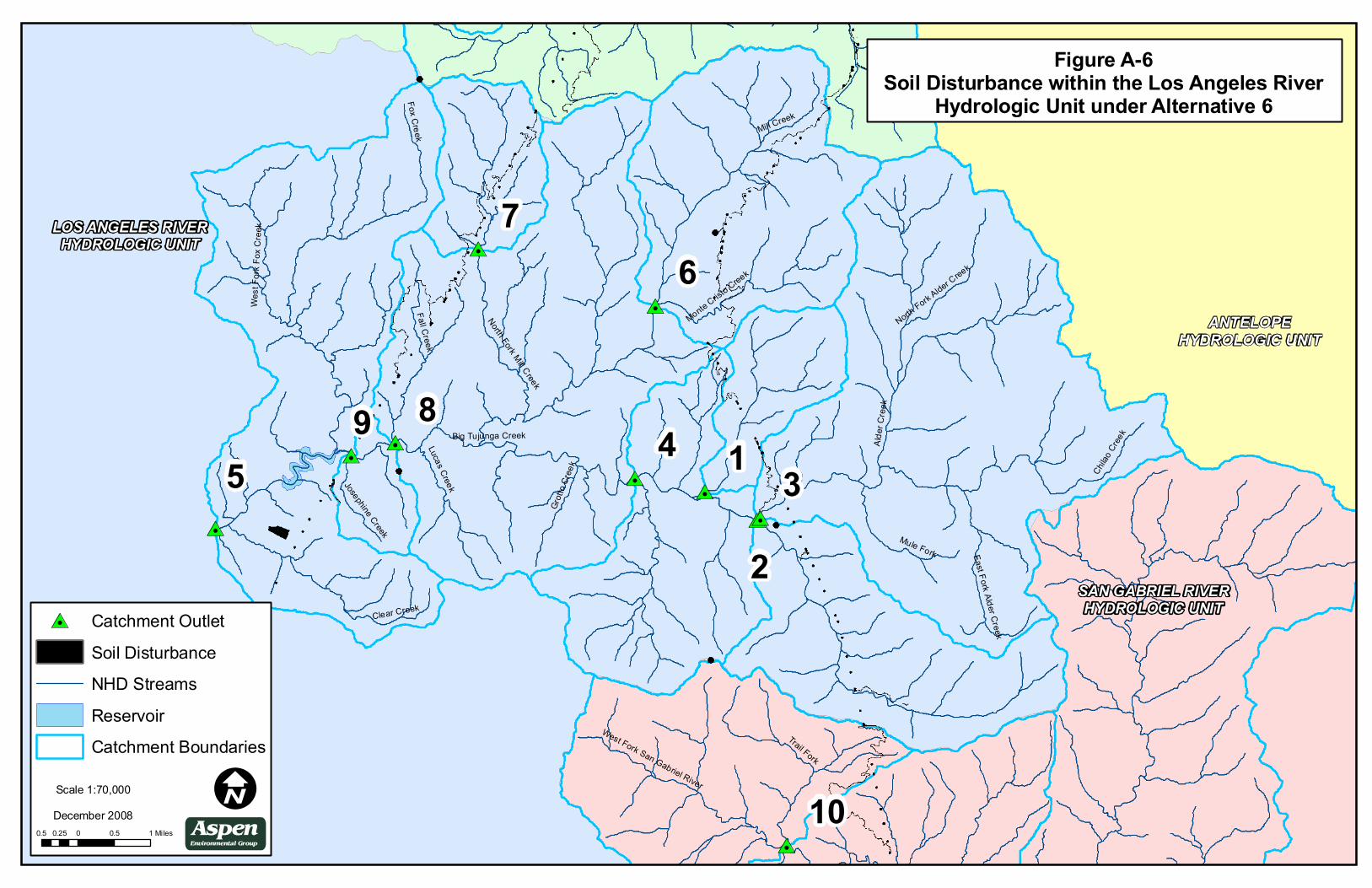
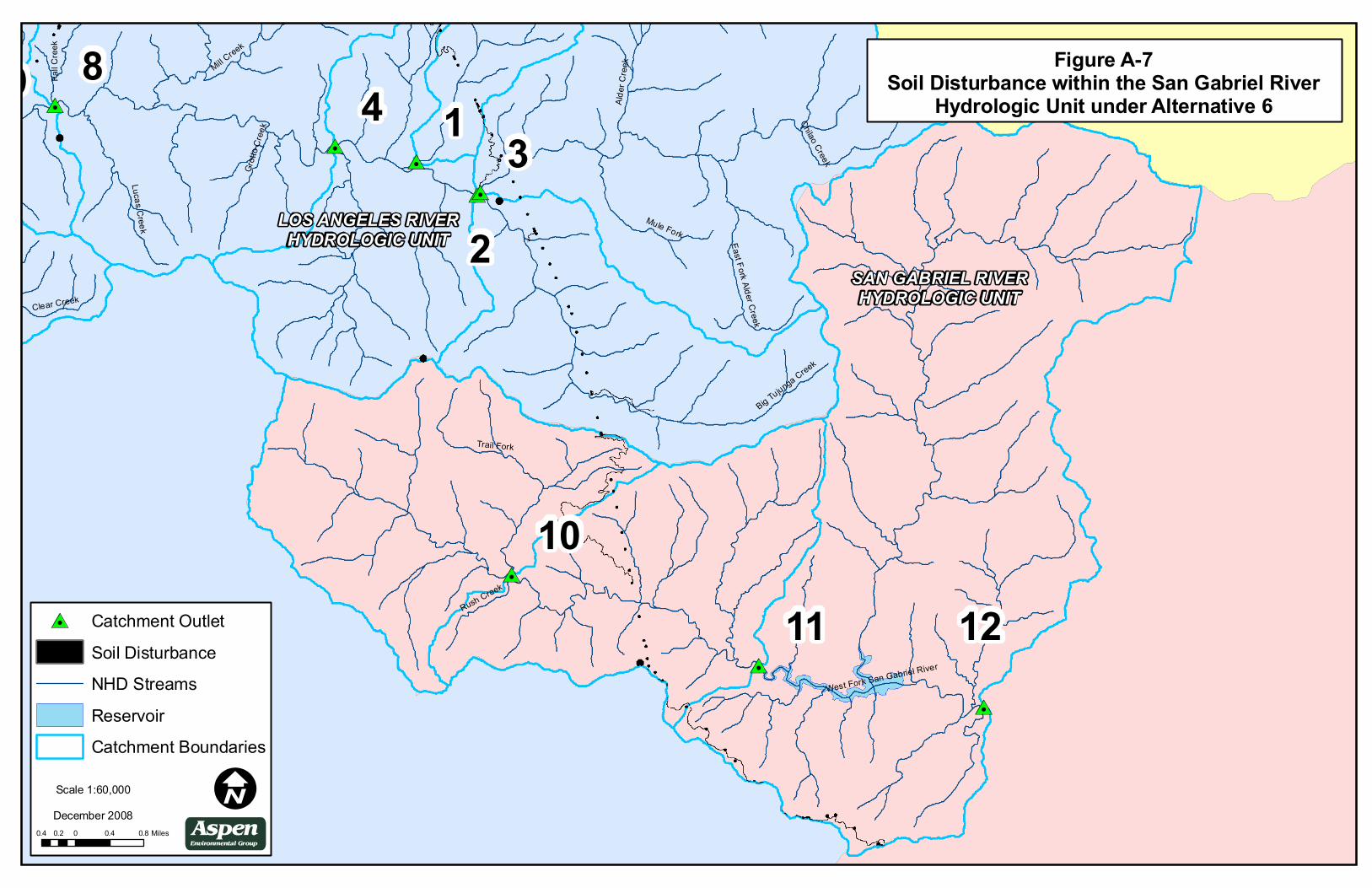
The EIR/EIS prepared for the proposed TRTP includes analysis of the proposed Project and six Project alternatives, including the No Project/Action Alternative. Among the identified Project alternatives, only Alternative 6 (Maximum Helicopter Construction on the ANF Alternative) differs from the proposed Project and other alternatives with regard to soil-disturbing activities that would occur on Forest lands. Therefore, this GIS-based erosion and sedimentation analysis addresses the effects of Alternative 2 (SCE’s proposed Project) and Alternative 6 (Maximum Helicopter Construction on the ANF Alternative) on the Forest. Soil disturbance associated with Alternative 2 is depicted in Figures 2 through 4, and soil disturbance associated with Alternative 6 is depicted in Figures 5 through 7.

Section 2 (Background) provides a description of the watershed and catchment areas that were defined for the purposes of this analysis. Section 3 (Methodology) includes a detailed description of the GIS technology and approach utilized in this analysis, including discussion of the primary model components (RUSLE and SEDMOD), as well as a description of the GIS model inputs and accuracy. Section 4 (Model Results and Discussion) and Section 5 (Summary and Recommendations) discuss the results of this analysis, and recommend actions to be applied during Project implementation that would minimize Project-related erosion, sedimentation and the related impacts to aquatic habitats and sensitive species.

2. BACKGROUND

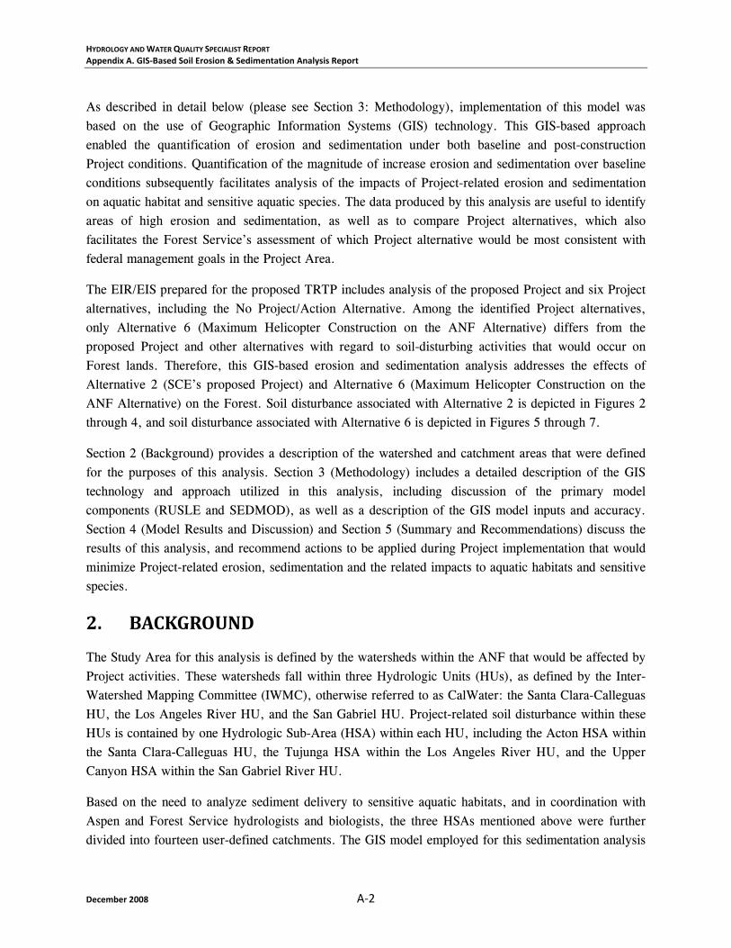
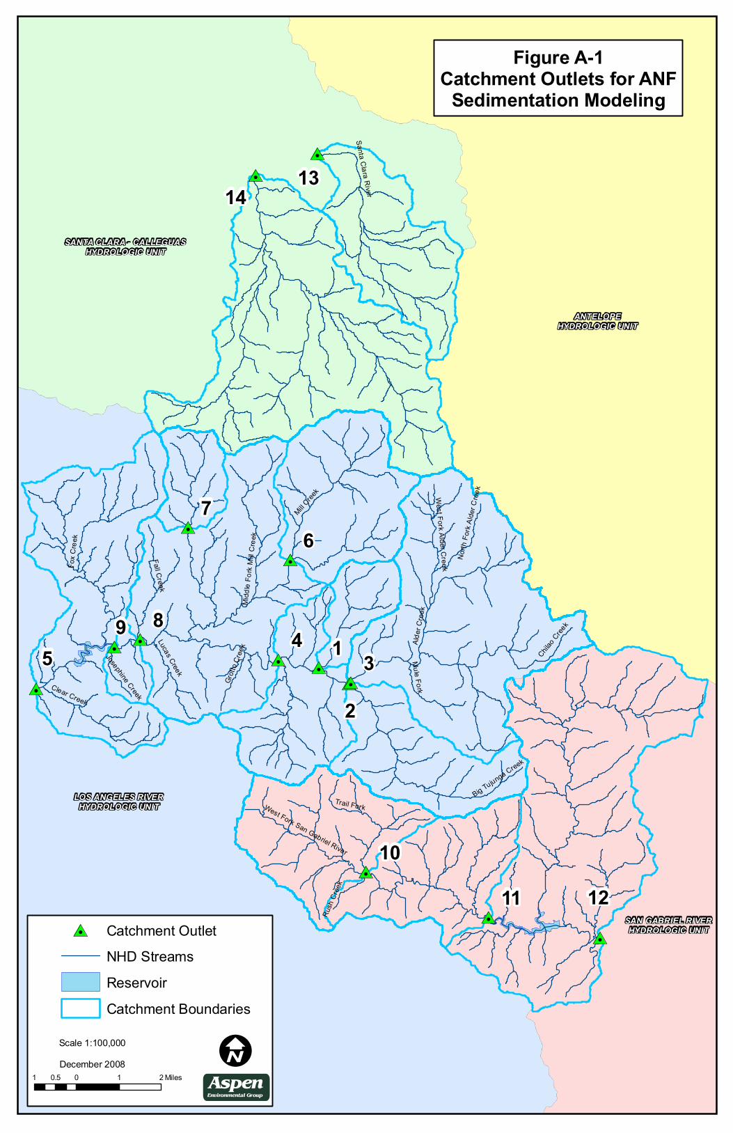
The Study Area for this analysis is defined by the watersheds within the ANF that would be affected by Project activities. These watersheds fall within three Hydrologic Units (HUs), as defined by the Inter-Watershed Mapping Committee (IWMC), otherwise referred to as CalWater: the Santa Clara-Calleguas HU, the Los Angeles River HU, and the San Gabriel HU. Project-related soil disturbance within these HUs is contained by one Hydrologic Sub-Area (HSA) within each HU, including the Acton HSA within the Santa Clara-Calleguas HU, the Tujunga HSA within the Los Angeles River HU, and the Upper Canyon HSA within the San Gabriel River HU.

Based on the need to analyze sediment delivery to sensitive aquatic habitats, and in coordination with Aspen and Forest Service hydrologists and biologists, the three HSAs mentioned above were further divided into fourteen user-defined catchments. The GIS model employed for this sedimentation analysis


A‐3 December 2008

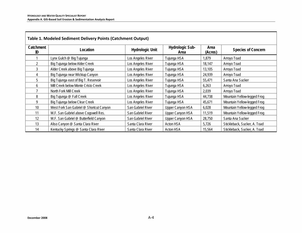
analyzed potential impacts at modeling points downstream of each of these fourteen catchments. All modeling points were selected based on coordination between Aspen and Forest Service biologists and hydrologists. Table 1 (Modeled Sediment Delivery Points (Catchment Output)), which is provided on the following page, summarizes the primary features of each modeled catchment area included in the Study Area.

As indicated in Table 1, the catchments that drain to each modeling point range in size from 2,000 acres to 55,000 acres. Five of the fourteen catchments are less than 6,300 acres, and several of the catchments are nested within larger catchments. The combined Study Area for this analysis totals approximately 105,500 acres. Figure 1 provides an overview of the Study Area and the location of the fourteen catchments and modeling points summarized above in Table 1. As indicated by Figure 1, these fourteen catchments are representative of the entire Study Area.

The soil characteristics and weather patterns within each catchment are critical factors that influence erosion and sedimentation. Soils within the Study Area are primarily formed either in alluvium or colluvium weathered from granitic or metamorphic bedrock, or in material weathered from the underlying bedrock (primarily granitic, metamorphic, and volcanic rocks). The climate within the Study Area varies between subtropical on the Pacific Ocean side of the San Gabriel Mountain range to semi-arid on the Mojave Desert side, with nearly all precipitation events occurring during the months of December through March. Precipitation during summer months is infrequent and rainless periods of several months are common. Average annual rainfall for the San Gabriel Mountains is approximately 27 inches (LADWP, 2005). Mount Islip, which is located along the crest of the San Gabriel Mountains, has annual rainfall highs of approximately 42 inches (SCE, 2007). The city of Acton, within the Acton HSA, receives an average annual precipitation of approximately nine inches (City-Data.com, 2007).

Susceptibility of sediment to transport and delivery is also largely affected by local terrain. Throughout the Study Area, terrain is highly varied. Some areas are characterized by steep slopes with minimal vegetation, while other areas are characterized by dense forests. Principal vegetative cover of the upper mountain areas in the Study Area consists of various species of brush and shrubs known as chaparral. Most trees found on mountain slopes are oak, with alder, willow, and sycamore found along streambeds at lower elevations. Pine, cedar, and juniper are found in ravines at higher elevations and along high mountain summits. These changes in vegetative cover and terrain are incorporated into the erosion and sedimentation model. (LADWP, 2005)


December 2008 A‐4

Table 1. Modeled Sediment Delivery Points (Catchment Output)

Catchment ID Location Hydrologic Unit Hydrologic Sub-

Area Area

(Acres) Species of Concern

1 Lynx Gulch @ Big Tujunga Los Angeles River Tujunga HSA 1,879 Arroyo Toad 2 Big Tujunga below Alder Creek Los Angeles River Tujunga HSA 18,147 Arroyo Toad 3 Alder Creek above Big Tujunga Los Angeles River Tujunga HSA 13,105 Arroyo Toad 4 Big Tujunga near Wickiup Canyon Los Angeles River Tujunga HSA 24,939 Arroyo Toad 5 Big Tujunga east of Big T. Reservoir Los Angeles River Tujunga HSA 55,471 Santa Ana Sucker 6 Mill Creek below Monte Cristo Creek Los Angeles River Tujunga HSA 6,263 Arroyo Toad 7 North Fork Mill Creek Los Angeles River Tujunga HSA 2,039 Arroyo Toad 8 Big Tujunga @ Fall Creek Los Angeles River Tujunga HSA 44,738 Mountain Yellow-legged Frog 9 Big Tujunga below Clear Creek Los Angeles River Tujunga HSA 45,671 Mountain Yellow-legged Frog 10 West Fork San Gabriel @ Shortcut Canyon San Gabriel River Upper Canyon HSA 6,028 Mountain Yellow-legged Frog 11 W.F. San Gabriel above Cogswell Res. San Gabriel River Upper Canyon HSA 11,519 Mountain Yellow-legged Frog 12 W.F. San Gabriel @ Butterfield Canyon San Gabriel River Upper Canyon HSA 28,750 Santa Ana Sucker 13 Aliso Canyon @ Santa Clara River Santa Clara River Acton HSA 5,726 Stickleback, Sucker, A. Toad 14 Kentucky Springs @ Santa Clara River Santa Clara River Acton HSA 15,564 Stickleback, Sucker, A. Toad


A‐5 December 2008

3. METHODOLOGY

As described in the preceding sections, this sedimentation analysis employed a GIS-integrated model to quantify the amount of sediment production and delivery that would occur within each of the fourteen affected hydrologic catchment areas as a result of construction activities under Alternative 2 (SCE’s Propose Project) and Alternative 6 (Maximum Helicopter Construction in the ANF). The use of a GIS-integrated approach in this analysis greatly reduced the time required for erosion and sedimentation modeling by removing the need for numerous field measurements and calculations. In addition, it was possible to achieve a finer resolution of the spatial distribution of the modeling results through GIS modeling than would have been possible through ground-based field calculations.

Model Selection. Based on a thorough review of scientific journal articles and other literature, it was determined that several erosion and sedimentation models would be viable for the purposes of this analysis. Each identified model utilized GIS software to analyze the interaction between environmental and Project-related factors, using existing and readily-available spatially distributed data. Through coordination between Aspen and Forest Service biologists and hydrologists, it was agreed that the Revised Universal Soil Loss Equation (RUSLE) model used in conjunction with a Spatially-Explicit Sediment Delivery Model (SEDMOD) would best satisfy the needs of this analysis. Sections 3.1 and 3.2, below, describe the RUSLE and SEDMOD methodologies employed for this analysis. Additionally, Section 3.3 provides a more detailed discussion of the GIS data inputs and associated level of accuracy for this analysis.

3.1 Revised Universal Soil Loss Equation (RUSLE)

The RUSLE is a modified version of the Universal Soil Loss Equation (USLE), which has been in use since the 1960s to measure soil loss from agricultural lands with relatively uniform slopes across a given plot. Over time, the original USLE was modified to account for terrain variability in features such as rangeland, mines, construction sites, and steeply-sloped topography. The RUSLE also includes modifications to certain USLE model factors, including slope length and slope steepness. In comparison with the original USLE, these modifications allow the RUSLE model to account for both convergent and divergent flow, thereby creating a more accurate portrayal of flow direction and accumulation over complex terrain. As a result, the RUSLE model is effective in measuring soil loss from land with variable topography, such as that found in the Study Area identified for this analysis.

The RUSLE model uses an empirical, GIS-integrated approach to assess rates of sediment transport and delivery. This model, which is based on observed data collected over several decades, is one of the most widely used and professionally accepted models for predicting annual erosion due to soil disturbance. Using a program developed by Mr. Van Remortel, the GIS-integrated RUSLE model generates soil and landform metrics through a set of computational executable programs using Arc Macro Language (AML) scripts and general-purpose programming language (C++) (Van Remortel, 2006). The GIS-integrated approach to employing the RUSLE model facilitated the assessment of


December 2008 A‐6

erosion and sedimentation on a whole-watershed scale, thereby allowing for the characterization of Project effects throughout the Study Area.

The output of the RUSLE model is an annual average rate of erosion and sedimentation; the output does not include a measure of soil loss that would occur during specific storm events. However, the RUSLE model does provide a percent increase in annual average erosion, which may be applied to any given storm event to predict the amount by which, on average, erosion caused by an individual storm event would increase over baseline conditions. The RUSLE model is appropriate for this analysis of ANF lands because it is able to provide a quantitative measurement of the erosion and sedimentation that would occur as a result of Project-related soil disturbance. These results can be used to describe the magnitude of potential impacts, and to assess differences between Project alternatives.

3.1.1 RUSLE Factors

The primary RUSLE model output is a quantification of long-term average annual soil loss expressed in tons per acre per year, as represented by the “A” factor. The A-factor, as the model output, is used to realistically approximate the amount of annual erosion, and is displayed as a spatially-distributed variable. This model output is determined by the product of five other factors, including the following:

• Rfactor: rainfall erosivity (i.e. how much of an influence rainfall plays in sediment production, or the intensity of rainfall events);

• Kfactor: soil erodibility (i.e. soil characteristics, cohesion, and susceptibility to erosion during rainfall events);

• LSfactor: slope length and slope steepness;

• Cfactor: land cover and management (i.e. characterization of land cover in terms of its influence on and/or resistance to erodibility); and

• Pfactor: support practice (i.e. Best Management Practices (BMPs) employed during Project activities).

As such, the RUSLE formula for assessing the annual average rate of erosion and sedimentation is as follows:

A = R * K * LS * C * P.

Each of the RUSLE factors is measured relative to a standard experimental plot of soil called the “unit plot”. Primary characteristics of the unit plot are summarized in Table 2 (RUSLE Unit Plot), which describes the LS-factor, C-factor, and P-factor.


A‐7 December 2008

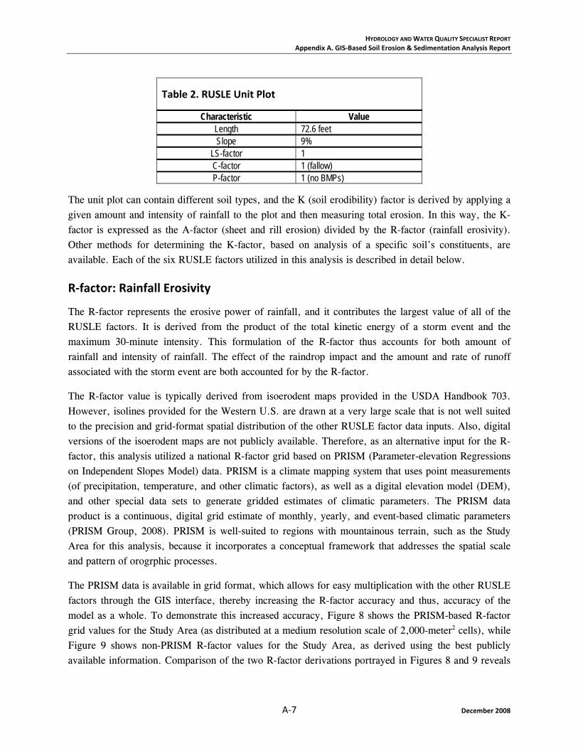
Table 2. RUSLE Unit Plot

Characteristic Value Length 72.6 feet Slope 9%

LS-factor 1 C-factor 1 (fallow) P-factor 1 (no BMPs)

The unit plot can contain different soil types, and the K (soil erodibility) factor is derived by applying a given amount and intensity of rainfall to the plot and then measuring total erosion. In this way, the K-factor is expressed as the A-factor (sheet and rill erosion) divided by the R-factor (rainfall erosivity). Other methods for determining the K-factor, based on analysis of a specific soil’s constituents, are available. Each of the six RUSLE factors utilized in this analysis is described in detail below.

R‐factor: Rainfall Erosivity

The R-factor represents the erosive power of rainfall, and it contributes the largest value of all of the RUSLE factors. It is derived from the product of the total kinetic energy of a storm event and the maximum 30-minute intensity. This formulation of the R-factor thus accounts for both amount of rainfall and intensity of rainfall. The effect of the raindrop impact and the amount and rate of runoff associated with the storm event are both accounted for by the R-factor.

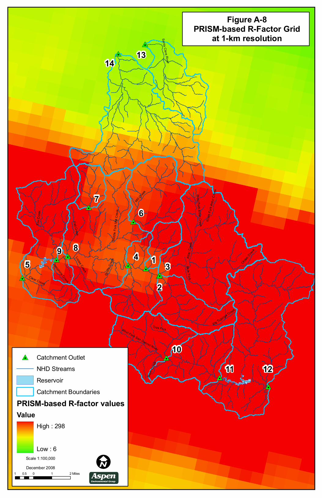
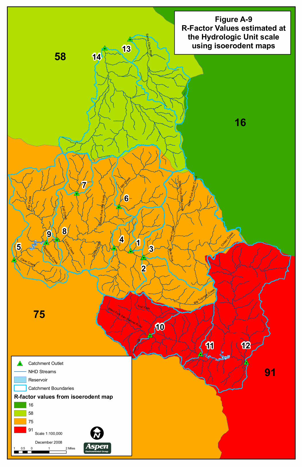
The R-factor value is typically derived from isoerodent maps provided in the USDA Handbook 703. However, isolines provided for the Western U.S. are drawn at a very large scale that is not well suited to the precision and grid-format spatial distribution of the other RUSLE factor data inputs. Also, digital versions of the isoerodent maps are not publicly available. Therefore, as an alternative input for the R-factor, this analysis utilized a national R-factor grid based on PRISM (Parameter-elevation Regressions on Independent Slopes Model) data. PRISM is a climate mapping system that uses point measurements (of precipitation, temperature, and other climatic factors), as well as a digital elevation model (DEM), and other special data sets to generate gridded estimates of climatic parameters. The PRISM data product is a continuous, digital grid estimate of monthly, yearly, and event-based climatic parameters (PRISM Group, 2008). PRISM is well-suited to regions with mountainous terrain, such as the Study Area for this analysis, because it incorporates a conceptual framework that addresses the spatial scale and pattern of orogrphic processes.

The PRISM data is available in grid format, which allows for easy multiplication with the other RUSLE factors through the GIS interface, thereby increasing the R-factor accuracy and thus, accuracy of the model as a whole. To demonstrate this increased accuracy, Figure 8 shows the PRISM-based R-factor grid values for the Study Area (as distributed at a medium resolution scale of 2,000-meter2 cells), while Figure 9 shows non-PRISM R-factor values for the Study Area, as derived using the best publicly available information. Comparison of the two R-factor derivations portrayed in Figures 8 and 9 reveals


December 2008 A‐8

that the coarser, non-PRISM estimate is deficient in portraying intra-watershed variation of the R-factor, as well as areas of high rainfall erosivity that occur in the higher mountain elevations. As such, it was determined that the PRISM data was the best available data to employ for this analysis.

K‐factor: Soil Erodibility

The K-factor represents soil susceptibility to erosion; in other words, the K-factor measures the ability of a particular soil type to resist erosion, or a soil type’s cohesion. A soil’s susceptibility to erosion is determined by the specific contents of the soil, including percentage of silt, sand, clay, and organic matter, as well as the soil structure and the permeability of the soil profile. The K-factor is expressed as a soil loss rate per erosion index unit for a specific soil, as measured on a standard RUSLE unit plot (please see Table 2). For this analysis, the K-factor was derived from a STATSGO (State Soil Geographic Database) grid for the State of California. Other soil data, such as SSURGO (Soil Survey Geographic Database), is more precise than STATSGO but is not available for the Project Study Area. In addition, the automated program used to implement the RUSLE through a GIS interface is not currently compatible with SSURGO data. Therefore, it was determined that the STATSGO grid data would be used for this analysis.

LS‐factor: Slope Length and Steepness

The LS-factor is a critical factor in accurately estimating soil erosion potential. It is defined as the ratio of soil loss from the Study Area to soil loss from a standardized RUSLE unit plot (please see Table 2). The LS-factor is a combination of two data sets: slope length (L), and slope steepness (S). Longer, steeper slopes produce higher overland flow velocities and higher rates of erosion. Slope length affects erosion potential more than slope steepness. Slope length is the distance from the origin of the overland flow to either the nearest stream or to a point where the slope changes sufficiently to allow for deposition.

When working with smaller geographic areas, the LS-factor can be calculated through the gathering and assessment of field measurements; however, because the Study Area defined for this analysis is large enough to require assessment on a regional scale, it was not possible to collect field measurements to the degree that would be necessary to accurately reflect the LS-factor for the entire Study Area. Instead, for the purposes of this analysis, a RUSLE-based grid of the LS-factor was calculated from a DEM through the model’s GIS interface. New algorithms derived by McCool et al. are incorporated into the automated program used with this GIS-based analysis, thereby accounting for convergent and divergent flow, which is important for accurately representing flow amount and velocity across complex terrain such as in the Study Area for this analysis (McCool, et al., 1989).

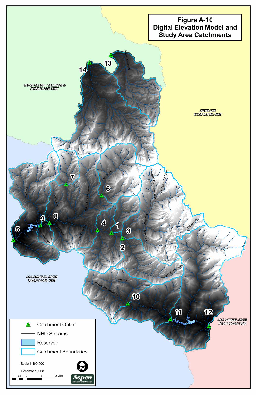
The DEM used in this analysis is the basic input from which the LS-factor grid is derived, as shown in Figure 10. Due to limitations in the processing ability of the automated LS-factor calculation program, the input must be in the form of an integer grid rather than a floating-point grid. Therefore, for this analysis, a non-floating-point DEM with a 10-meter cell size was used. This 10-meter cell-size grid was


A‐9 December 2008

first clipped to the hydrologically-defined watershed boundary, in order to reduce processing time by eliminating unnecessary data, while also preventing slope length calculation errors. In addition, the DEM used for this analysis was of high quality, did not contain artificial ‘steps’ from mosaic errors, and did not include changes common of ‘smoothing’ programs.

The micro-relief of the digital landscape created for this model was limited to the resolution of the DEM used, which was built of cells 10 meters by 10 meters wide. Therefore, all roads in the Study Area were represented by series of individual cells, each of which was 10 meters wide. Forest System roads relevant to the Study Area for this analysis are actually five meters wide and, therefore, this analysis overestimated the width of roads by approximately five meters. Roads that are cut across hillsides were represented in the model by slope changes but because road width was over-estimated by the 10-meter DEM, such changes in slope were not exactly representative of ground conditions. However, in the absence of a more precise DEM, the 10-meter DEM was considered to be acceptable for the purposes of this analysis.

In order to create a model where surface water flow accumulates within logical channels without digital “sinks”, or depressions with no logical outflow, an iterative routine was employed to “fill” such depressions in the DEM prior to its application in the RUSLE (Hickey et al., 1994). The fill routine that was applied for this analysis was built into the original AMLs developed by Mr. Rick Van Remortel, which are described above in Section 3.1. In addition, an application called ArcHydro was used to calculate a flow direction grid for the Study Area, based on the steepest descent (slope) from each 10-meter cell in the DEM (Maidment, 2002). Using the GIS interface, ArcHydro allows water to “exit” each cell in one of eight directions (cardinal and half-cardinal). It is this multi-directional flow analysis that allows for convergent and divergent flows to be represented in the model. Please see Figure 11 for a representation of this routine.

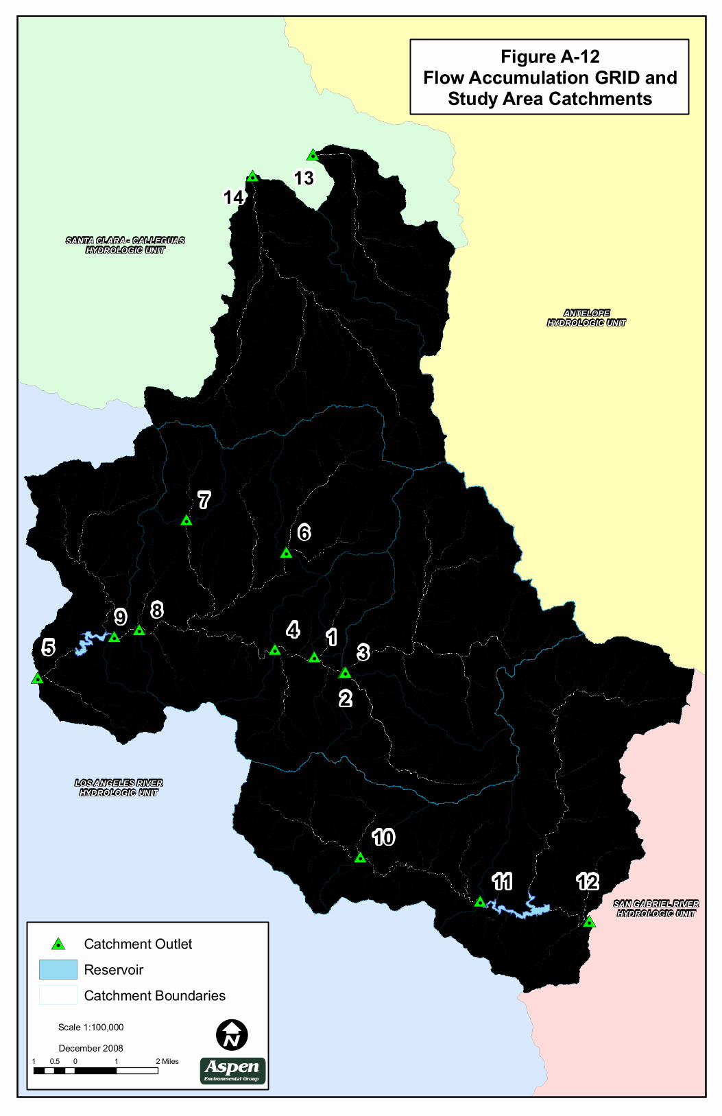
Once the flow direction grid has been derived using ArcHydro, slope length was investigated. As water flows further down the watershed and begins to concentrate towards the outlet point (where sedimentation is measured by the model), the flow amount accumulates and increases in volume. This accumulation of flow was represented as a flow accumulation grid, which is depicted in Figure 12. The flow accumulation grid was used to create a hydrologically defined stream network. For accurate calculation of slope length, the program needed to distinguish between erosion and deposition. Erosion and deposition both depend on slope steepness, which is the main determinant of flow velocity. These processes are also a function of sediment concentration in the water. If water is fully saturated with sediment, it must maintain velocity in order to prevent deposition. Conversely, if water is not very saturated with sediment, then changes in slope are less likely to result in deposition. The automated program (SEDMOD, as described below in Section 3.2) that calculates both erosion and deposition uses a slope “cutoff factor” to determine when deposition begins. This method accounts for changes in slope from cell to cell. For this analysis, the following default cutoff values were used:


December 2008 A‐10

(1) On slopes steeper than 5%, a 50% change in slope gradient was required to initiate deposition;

(2) On slopes gentler than 5%, a 30% change in slope gradient was required to initiate deposition.

By incorporating a cutoff factor into the LS calculation, the model more accurately describes erosion by avoiding huge slope length numbers which would grossly bias the calculations upward.

C‐factor: Land Cover and Management

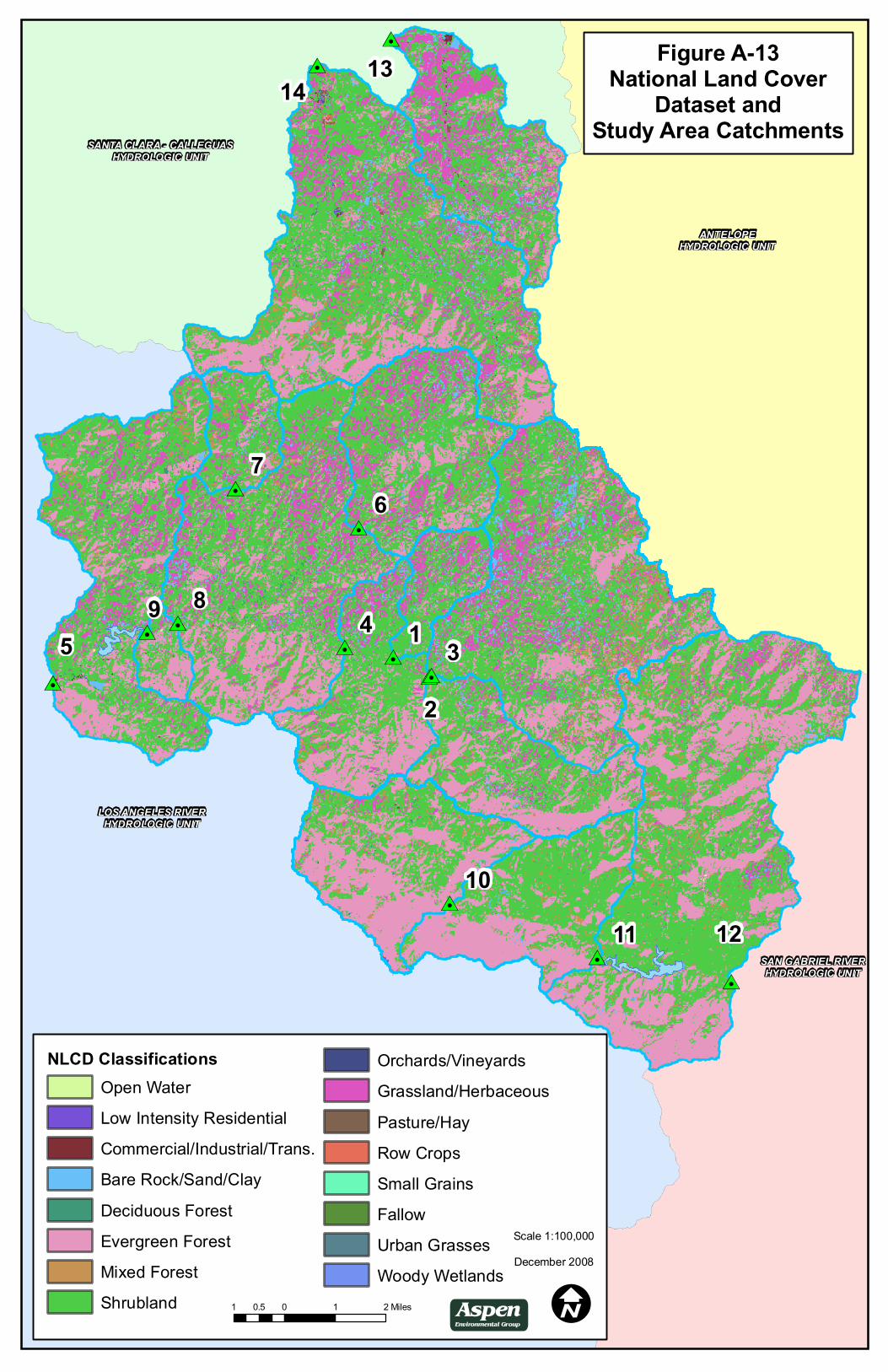
The C-factor represents crop or land cover management, and is represented as the ratio of soil loss from the Study Area to soil loss from an identical area that is left fallow and tilled parallel to the slope. This factor accounts for the effect that plants and soil cover have on soil loss. For the purposes of this analysis, the C-factor was derived from a National Land Cover Dataset (NLCD) grid that was clipped to the Study Area boundary, as shown in Figure 13. The C-factor is particularly useful for this analysis because, unlike other factors that are environment-dependent and cannot be altered (such as topography or rainfall), the C-factor can be used to represent soil-disturbing activities included under the proposed Project and Project alternatives and it is therefore altered as necessary to reflect Project activities. As such, the C-factor is the main mechanism by which the differences between project alternatives are modeled.

One of the major soil-disturbing activities associated with construction of the proposed Project is widening and improvement of Forest System roads in the ANF. The intensity of road improvement included as part of construction varies across the Project alternatives, which accounts for the primary changes in predicted annual average erosion and sedimentation for each alternative. In order to represent the effects of road improvements and other soil disturbance associated with proposed construction activities, a C-factor value of 0.98 was used for new or improved roadways in the Forest, including access roads and spur roads. In addition, due to similarities in the types of land disturbing activities associated with road improvements and the installation of helicopter fly yards, marshalling yards, helicopter landing pads, and pulling/stringing sites, the same C-factor value was used for each of these areas. This C-factor value was derived from NLCD land classification 31, which represents “bare rock/sand/clay, barren land” and is therefore also representative of recently graded sites (NLCD, 2006).

P‐factor: Support Practice

The P-factor is the support or land management factor, and is typically used to account for such practices as contour farming, terracing, and strip cropping. The P-factor typically ranges from 0.0 to 1.0, with a P-factor value of 1.0 representing forested land where agricultural support practices, such as contour tilling, are not used. In order to represent parts of the Study Area that would not be disturbed by Project activities, a P-factor value of 1.0 was used. In literature on this topic, it has been reported that P-factor values of 1.3 are appropriate for blade-graded soils; however, due to the overestimation of road width (ten meters in the DEM versus five meters on the ground) already


A‐11 December 2008

incorporated into this analysis as a result of the 10-meter cell DEM used to represent the LS-factor, this high P-factor of 1.3 was not utilized. Additionally, there is a general lack of consensus in the professional community as to the appropriateness of using a P-factor value greater than 1.0. Therefore, for the purposes of this analysis, the application of a P-factor value of 1.0 to areas of soil disturbance is considered an adjustment to the model that accounts for the overestimation of road widths.

On the scale of 0.0 to 1.0, recent work has resulted in the development of P-factor values that represent construction best management practices (BMPs) such as silt fences, fiber rolls, and sedimentation basins (Dion, 2002; Galetovic et al., 1998). For this analysis a P-factor of 0.4 was used as a reasonable and conservative representation of BMPs. The average value of several support practices on a 10-15% gradient slope is 0.5, but it was determined that 0.4 would be an appropriate value to use in order to account for the over-estimation of road widths, as described above.

3.2 SpatiallyExplicit Sediment Delivery Model (SEDMOD)

Sedimentation at a specific point in the watershed is determined by the total upland erosion minus any deposition that has occurred along the way, where “deposition” refers to soils that have eroded as a result of disturbance, but are not transported all the way to a stream channel or a watershed outlet. Therefore, in order to accurately quantify sediment deposition, it is essential to also quantify deposition within the catchment basins. For the purposes of this analysis, a Spatially-Explicit Sediment Delivery Model (SEDMOD) was used in conjunction with the RUSLE in order to address sediment not transported all the way to the selected modeling points in the Study Area. SEDMOD is run through the 6th AML built into Rick Van Remortel’s set of computational executable programs described above (please see the introduction under Section 3.1). Deposition of eroded soil is influenced by several factors, including soil-particle size, flow rate of the storm runoff, and changes in slope steepness (this is the slope cutoff factor that is described above for the LS-factor). As with the RUSLE, the SEDMOD assesses deposition using an integrated GIS approach, and is run in sequence after the RUSLE factors have been determined.

3.3 GIS Data Input and Accuracy

The GIS-based approach applied to this sedimentation analysis provides a representation of the spatial distribution of Project impacts, which allows scientists and decision-makers to accurately identify areas where BMPs and mitigation measures should be applied to reduce the impacts of sediment delivery. Additionally, this GIS-based approach facilitates the analysis of sedimentation impacts on a regional scale, which would otherwise be prohibitively data intensive. Collection of the number of field measurements that would be required to provide the same resolution of spatially-distributed results would not be feasible to achieve within the timeframe specified for this analysis. The RUSLE and SEDMOD applications utilized for this analysis were integrated through ESRI’s ArcGIS 9.3 Desktop software, using an ArcInfo license. Several components of this software package were employed in this analysis, including ArcMap, ArcCatalog, and ArcInfo Workstation. As described in Section 3.1, AMLs



developed by Mr. Rick Van Remortel include the commands necessary to implement the RUSLE and SEDMOD.

This analysis utilized both of the two main types of GIS data formats for model inputs: vector data and raster data. “Vector” data is comprised of x-y coordinate representations of locations on the earth that take the form of single points, strings of points (lines or arcs), or closed lines (polygons). Examples of vector data used in this analysis include streams, monitoring points, and watershed boundaries. In contrast, “raster” data is cell data arranged in a regular grid pattern in which each unit (pixel or cell) in the grid is assigned an identifying value based on its characteristics. Examples of raster data used in this analysis include elevation grids, rainfall distribution, and soil type distribution.

The accuracy of the data outputs produced by this analysis is directly tied to the quality of the data inputs. For this analysis, two primary data inputs that are used by both the RUSLE and the SEDMOD formulas were employed, including a digital elevation grid, or DEM, and National Hydrography Dataset (NHD) stream network data. This analysis used a DEM that was produced using several different USGS DEMs that were digitally combined to form one DEM that covered the entire Project Study Area. Each of the original DEMs were based on 7.5-minute USGS quadrangle maps and were combined using Globalmapper software. The resolution of the combined DEM, which portrayed all fourteen catchments in this analysis, was a 10-meter square cell, and elevation values were represented as discrete, rather than floating-point, data.

As mentioned, another important data input used by both models is the stream network provided by the NHD. This analysis used the High-Resolution NHD data which, as with the DEMs, is based on 7.5-minute USGS quadrangle maps. Blue lines from the USGS quadrangle maps were digitized to create the NHD vector file of streams. Although the vector file of streams does accurately represent the USGS data (from the quadrangle maps), the resolution of this accuracy is limited to the 1:24,000 scale at which the streams were digitized. Also, although the streams are considered to be cartographically correct, the stream vector file contains many small gaps and loops, and does not maintain network connectivity. Therefore, for this analysis, the NHD streams were first edited to form a cohesive and hydrologically accurate network before being applied to the model.

The RUSLE and the SEDMOD are both based on the flow of water and loose soil over a digital representation of the Earth’s surface; therefore, the accuracy of the DEMs and the NHD data described above are essential to the process of delineating hydrologically correct watersheds. Any missing or extraneous portions of the digital watershed representations utilized in this analysis could lead to a variety of inaccuracies in the model, such as interrupted or truncated slope lengths and flow lines or overestimated slope lengths, in addition to greatly extended processing times. For this analysis, delineation of precise, hydrologically correct watersheds was accomplished through the use of an ArcGIS extension called ArcHydro, developed by Dr. Maidment at the Center for Research in Water Resources (Maidment, 2002). Using ArcHydro, watersheds were defined through a multi-step process that is based primarily on analysis of the DEM, using the NHD data to increase the influence of a



known stream network. Several grids (data sets) were derived from the initial DEM, including flow direction, flow accumulation, and stream definition. From these grids, hydrologically correct catchments were derived based on user-defined outlet points, and subsequently used as “cookie-cutters” to clip the RUSLE factor grids prior to running the model calculations. As such, model calculations only consider data relevant to the identified Study Area.

4. Model Results and Discussion

The results of the RUSLE/SEDMOD analysis include quantification of average annual sediment production and delivery under the following conditions for each of the fourteen identified outlet points:

• Baseline (existing conditions without Project‐related disturbance);

• Alternative 2 (SCE’s Proposed Project) without Best Management Practices (BMPs);

• Alternative 2 with application of BMPs;

• Alternative 6 (Maximum Helicopter Construction in the ANF) without BMPs; and

• Alternative 6 with application of BMPs.

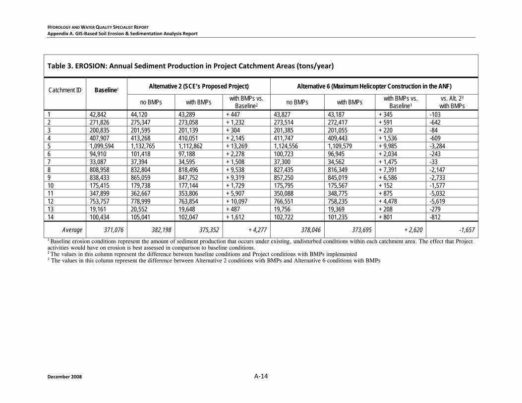
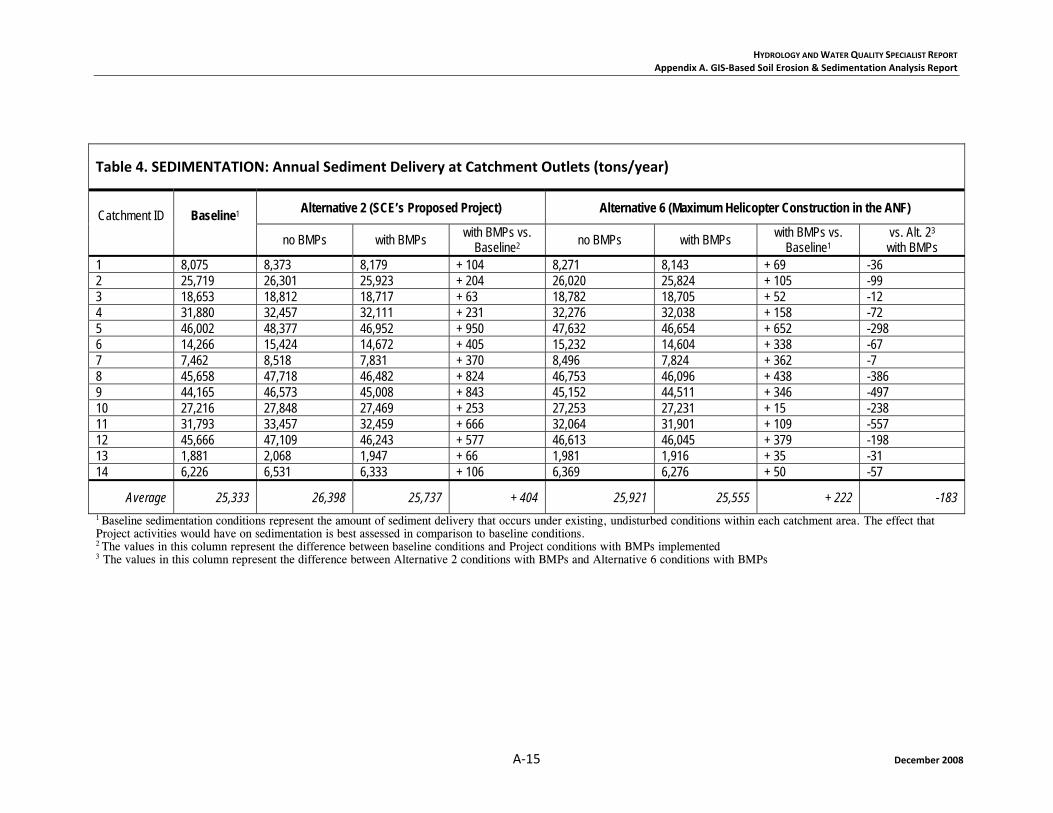
The data provided by the RUSLE and SEDMOD model outputs is presented below in Table 3 (Erosion: Annual Sediment Production in Project Catchment Areas (tons/year)) and in Table 4 (Sedimentation: Annual Sediment Delivery at Catchment Outlets (tons/year)). These tables provide the RUSLE and SEDMOD-calculated amounts of sediment production and delivery, respectively, for each of the conditions listed above. In addition, these tables provide the calculated differences in sediment production and delivery between the modeled alternatives and baseline conditions. The results presented in Tables 3 and 4 are most usefully considered as a general indicator of Project-related increases in sediment load to streams, rather than as an exact amount in tons. The data presented in Tables 3 and 4 are discussed in further detail below, following Table 4.

As mentioned above, baseline conditions represent the natural processes of sediment transport and delivery that are currently and naturally occurring in the Project Area, absent any Project-related disturbance. The results presented in Tables 3 and 4 indicate that neither Alternative 2 nor Alternative 6 would result in substantially greater rates of sediment delivery, or sedimentation, compared to baseline conditions. The annual average baseline erosion amounts reported above are consistent with values reported in professional literature, especially considering the steep terrain, intense rainfall, and chaparral cover of the Study Area.



Table 3. EROSION: Annual Sediment Production in Project Catchment Areas (tons/year)

Catchment ID Baseline1 Alternative 2 (SCE’s Proposed Project) Alternative 6 (Maximum Helicopter Construction in the ANF)

no BMPs with BMPs with BMPs vs. Baseline2 no BMPs with BMPs with BMPs vs.

Baseline1 vs. Alt. 23 with BMPs

1 42,842 44,120 43,289 + 447 43,827 43,187 + 345 -103 2 271,826 275,347 273,058 + 1,232 273,514 272,417 + 591 -642 3 200,835 201,595 201,139 + 304 201,385 201,055 + 220 -84 4 407,907 413,268 410,051 + 2,145 411,747 409,443 + 1,536 -609 5 1,099,594 1,132,765 1,112,862 + 13,269 1,124,556 1,109,579 + 9,985 -3,284 6 94,910 101,418 97,188 + 2,278 100,723 96,945 + 2,034 -243 7 33,087 37,394 34,595 + 1,508 37,300 34,562 + 1,475 -33 8 808,958 832,804 818,496 + 9,538 827,435 816,349 + 7,391 -2,147 9 838,433 865,059 847,752 + 9,319 857,250 845,019 + 6,586 -2,733 10 175,415 179,738 177,144 + 1,729 175,795 175,567 + 152 -1,577 11 347,899 362,667 353,806 + 5,907 350,088 348,775 + 875 -5,032 12 753,757 778,999 763,854 + 10,097 766,551 758,235 + 4,478 -5,619 13 19,161 20,552 19,648 + 487 19,756 19,369 + 208 -279 14 100,434 105,041 102,047 + 1,612 102,722 101,235 + 801 -812

Average 371,076 382,198 375,352 + 4,277 378,046 373,695 + 2,620 -1,657 1 Baseline erosion conditions represent the amount of sediment production that occurs under existing, undisturbed conditions within each catchment area. The effect that Project activities would have on erosion is best assessed in comparison to baseline conditions.

2 The values in this column represent the difference between baseline conditions and Project conditions with BMPs implemented 3 The values in this column represent the difference between Alternative 2 conditions with BMPs and Alternative 6 conditions with BMPs



Table 4. SEDIMENTATION: Annual Sediment Delivery at Catchment Outlets (tons/year)

Catchment ID Baseline1 Alternative 2 (SCE’s Proposed Project) Alternative 6 (Maximum Helicopter Construction in the ANF)

no BMPs with BMPs with BMPs vs. Baseline2 no BMPs with BMPs with BMPs vs.

Baseline1 vs. Alt. 23 with BMPs

1 8,075 8,373 8,179 + 104 8,271 8,143 + 69 -36 2 25,719 26,301 25,923 + 204 26,020 25,824 + 105 -99 3 18,653 18,812 18,717 + 63 18,782 18,705 + 52 -12 4 31,880 32,457 32,111 + 231 32,276 32,038 + 158 -72 5 46,002 48,377 46,952 + 950 47,632 46,654 + 652 -298 6 14,266 15,424 14,672 + 405 15,232 14,604 + 338 -67 7 7,462 8,518 7,831 + 370 8,496 7,824 + 362 -7 8 45,658 47,718 46,482 + 824 46,753 46,096 + 438 -386 9 44,165 46,573 45,008 + 843 45,152 44,511 + 346 -497 10 27,216 27,848 27,469 + 253 27,253 27,231 + 15 -238 11 31,793 33,457 32,459 + 666 32,064 31,901 + 109 -557 12 45,666 47,109 46,243 + 577 46,613 46,045 + 379 -198 13 1,881 2,068 1,947 + 66 1,981 1,916 + 35 -31 14 6,226 6,531 6,333 + 106 6,369 6,276 + 50 -57

Average 25,333 26,398 25,737 + 404 25,921 25,555 + 222 -183 1 Baseline sedimentation conditions represent the amount of sediment delivery that occurs under existing, undisturbed conditions within each catchment area. The effect that Project activities would have on sedimentation is best assessed in comparison to baseline conditions.

2 The values in this column represent the difference between baseline conditions and Project conditions with BMPs implemented 3 The values in this column represent the difference between Alternative 2 conditions with BMPs and Alternative 6 conditions with BMPs



It is critical to note that the natural variation in sediment delivery to streams in the Study Area is substantially greater than the modeled sedimentation increases that would result from Project activities. Most precipitation in the Study Area occurs during only four months of the year, with storm events that generally tend to be both large and intense. During most of the year, little to no sediment is delivered to waterways in the Study Area. But during a large storm event, a huge amount of sediment may be transported and delivered directly into aquatic habitat. This variation is completely independent of human activity and is part of the natural morphology of the Study Area. Therefore, an increase in annual average sediment delivery of up to ten percent would not be considered substantial, in comparison with the magnitude of natural variation of sediment transport and delivery that presently occurs in the Study Area. Additionally, aquatic species in the Study Area are presently acclimated to the hydrologic changes in the aquatic environment that occur as a result of intense storm events. As such, it is not expected that a temporary increase in sediment transport and delivery such as would occur under Alternative 2 or Alternative 6 would affect the viability of aquatic species on the ANF.

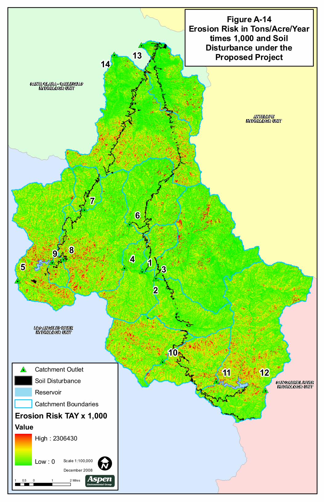
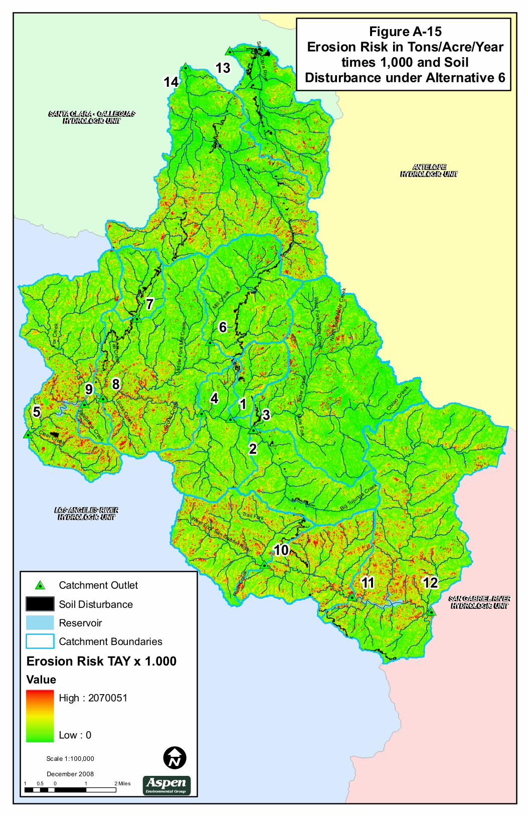
The results portrayed in Tables 3 and 4 are particularly useful in two ways. First, these calculations allow for a comparison of alternatives and baseline conditions, both before and after implementation of Best Management Practices, and secondly, these calculations provide spatially distributed data which indicates where (which outlet point) and to what magnitude (annual average sedimentation) the impacts of Project-related soil disturbance would occur. The cell by cell representation of erosion and sedimentation prepared in this RUSLE/SEDMOD model allows scientists and decision makers to focus their mitigation efforts on areas of high risk, and to implement BMPs or Project modifications that take into account the most high-risk areas, i.e. the areas where the increase in sedimentation would have the highest potential to affect aquatic habitat and species. Figures 14 and 15 provide a visual representation of the spatial distribution of erosion risk within the Study Area.

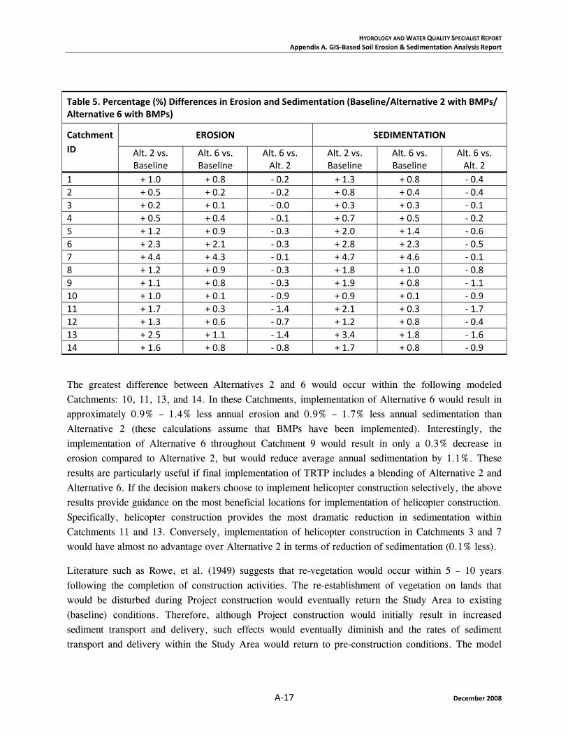
As indicated in the tables above, the implementation of BMPs during Project construction activities would substantially reduce sediment transport and delivery in the Study Area. Table 5 (Percentage Differences in Erosion and Sedimentation (Baseline / Alternative 2 with BMPs / Alternative 6 with BMPs), presented below, provides a summary of differences between baseline conditions, Alternative 2 with BMPs, and Alternative 6 with BMPs. Additionally, as reflected in Tables 3 and 4, the rates of sediment transport and delivery under Alternative 2 would be greater than under Alternative 6, both with and without the implementation of BMPs. Table 5, presented below, provides a percentage calculation of differences between the alternatives, which can be used to identify catchments where the differences would be most substantial.

As indicated in Table 5, both Alternative 2 and Alternative 6 would result in increases from baseline conditions for both erosion and sedimentation and, as previously mentioned, the calculated amounts of erosion and sedimentation that would occur under Alternative 6 are lower than those that would occur under Alternative 2. However, as noted in Table 5, the differences between Alternatives 2 and 6 are not considered to be substantial.



Table 5. Percentage (%) Differences in Erosion and Sedimentation (Baseline/Alternative 2 with BMPs/ Alternative 6 with BMPs)

Catchment ID

EROSION SEDIMENTATION

Alt. 2 vs. Baseline

Alt. 6 vs. Baseline

Alt. 6 vs. Alt. 2

Alt. 2 vs. Baseline

Alt. 6 vs. Baseline

Alt. 6 vs. Alt. 2

1 + 1.0 + 0.8 ‐ 0.2 + 1.3 + 0.8 ‐ 0.4 2 + 0.5 + 0.2 ‐ 0.2 + 0.8 + 0.4 ‐ 0.4 3 + 0.2 + 0.1 ‐ 0.0 + 0.3 + 0.3 ‐ 0.1 4 + 0.5 + 0.4 ‐ 0.1 + 0.7 + 0.5 ‐ 0.2 5 + 1.2 + 0.9 ‐ 0.3 + 2.0 + 1.4 ‐ 0.6 6 + 2.3 + 2.1 ‐ 0.3 + 2.8 + 2.3 ‐ 0.5 7 + 4.4 + 4.3 ‐ 0.1 + 4.7 + 4.6 ‐ 0.1 8 + 1.2 + 0.9 ‐ 0.3 + 1.8 + 1.0 ‐ 0.8 9 + 1.1 + 0.8 ‐ 0.3 + 1.9 + 0.8 ‐ 1.1 10 + 1.0 + 0.1 ‐ 0.9 + 0.9 + 0.1 ‐ 0.9 11 + 1.7 + 0.3 ‐ 1.4 + 2.1 + 0.3 ‐ 1.7 12 + 1.3 + 0.6 ‐ 0.7 + 1.2 + 0.8 ‐ 0.4 13 + 2.5 + 1.1 ‐ 1.4 + 3.4 + 1.8 ‐ 1.6 14 + 1.6 + 0.8 ‐ 0.8 + 1.7 + 0.8 ‐ 0.9

The greatest difference between Alternatives 2 and 6 would occur within the following modeled Catchments: 10, 11, 13, and 14. In these Catchments, implementation of Alternative 6 would result in approximately 0.9% – 1.4% less annual erosion and 0.9% – 1.7% less annual sedimentation than Alternative 2 (these calculations assume that BMPs have been implemented). Interestingly, the implementation of Alternative 6 throughout Catchment 9 would result in only a 0.3% decrease in erosion compared to Alternative 2, but would reduce average annual sedimentation by 1.1%. These results are particularly useful if final implementation of TRTP includes a blending of Alternative 2 and Alternative 6. If the decision makers choose to implement helicopter construction selectively, the above results provide guidance on the most beneficial locations for implementation of helicopter construction. Specifically, helicopter construction provides the most dramatic reduction in sedimentation within Catchments 11 and 13. Conversely, implementation of helicopter construction in Catchments 3 and 7 would have almost no advantage over Alternative 2 in terms of reduction of sedimentation (0.1% less).

Literature such as Rowe, et al. (1949) suggests that re-vegetation would occur within 5 – 10 years following the completion of construction activities. The re-establishment of vegetation on lands that would be disturbed during Project construction would eventually return the Study Area to existing (baseline) conditions. Therefore, although Project construction would initially result in increased sediment transport and delivery, such effects would eventually diminish and the rates of sediment transport and delivery within the Study Area would return to pre-construction conditions. The model



calculations presented in the preceding tables represents the worst-case (most conservative) scenario, where no re-vegetation has occurred.

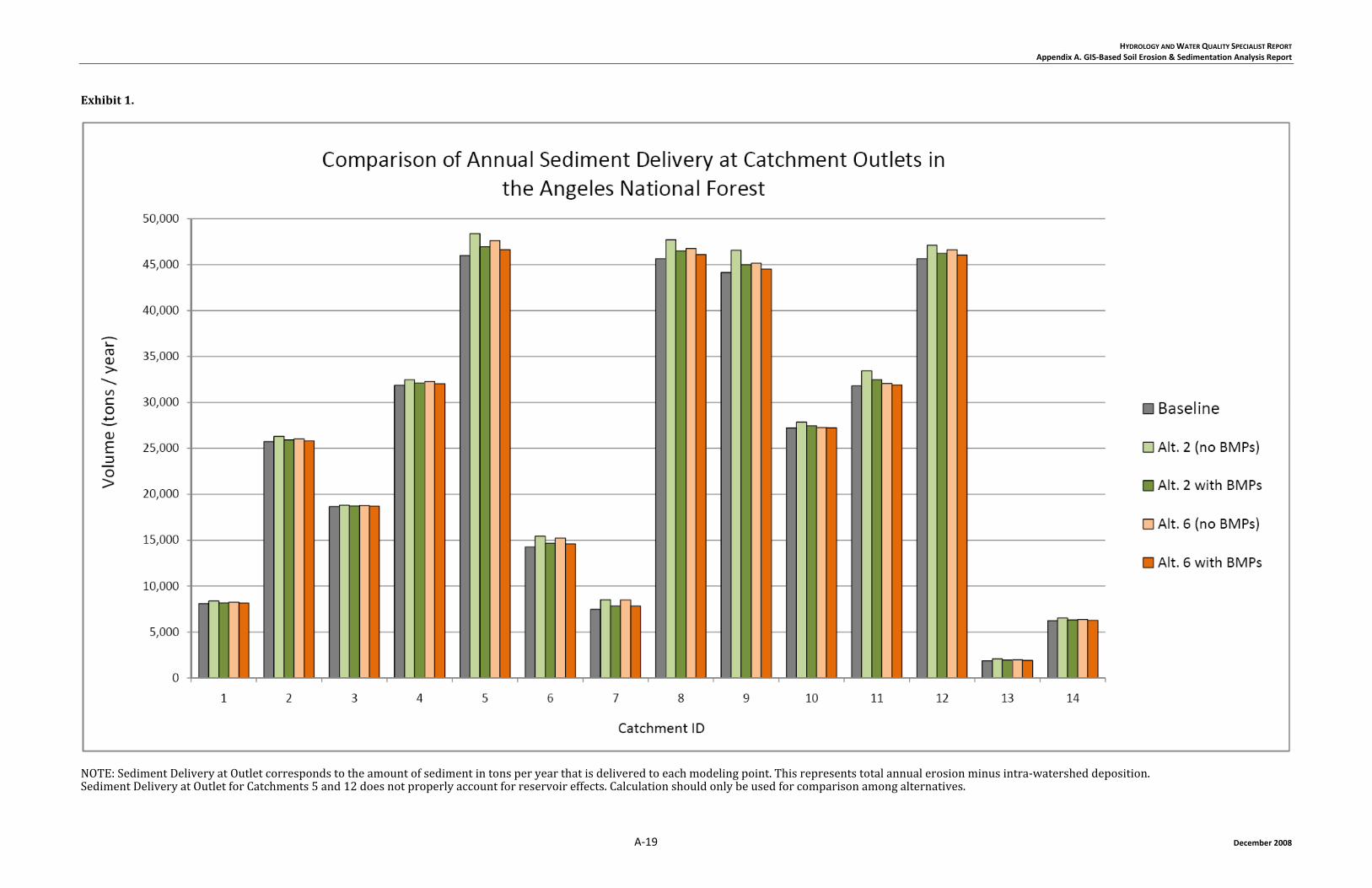
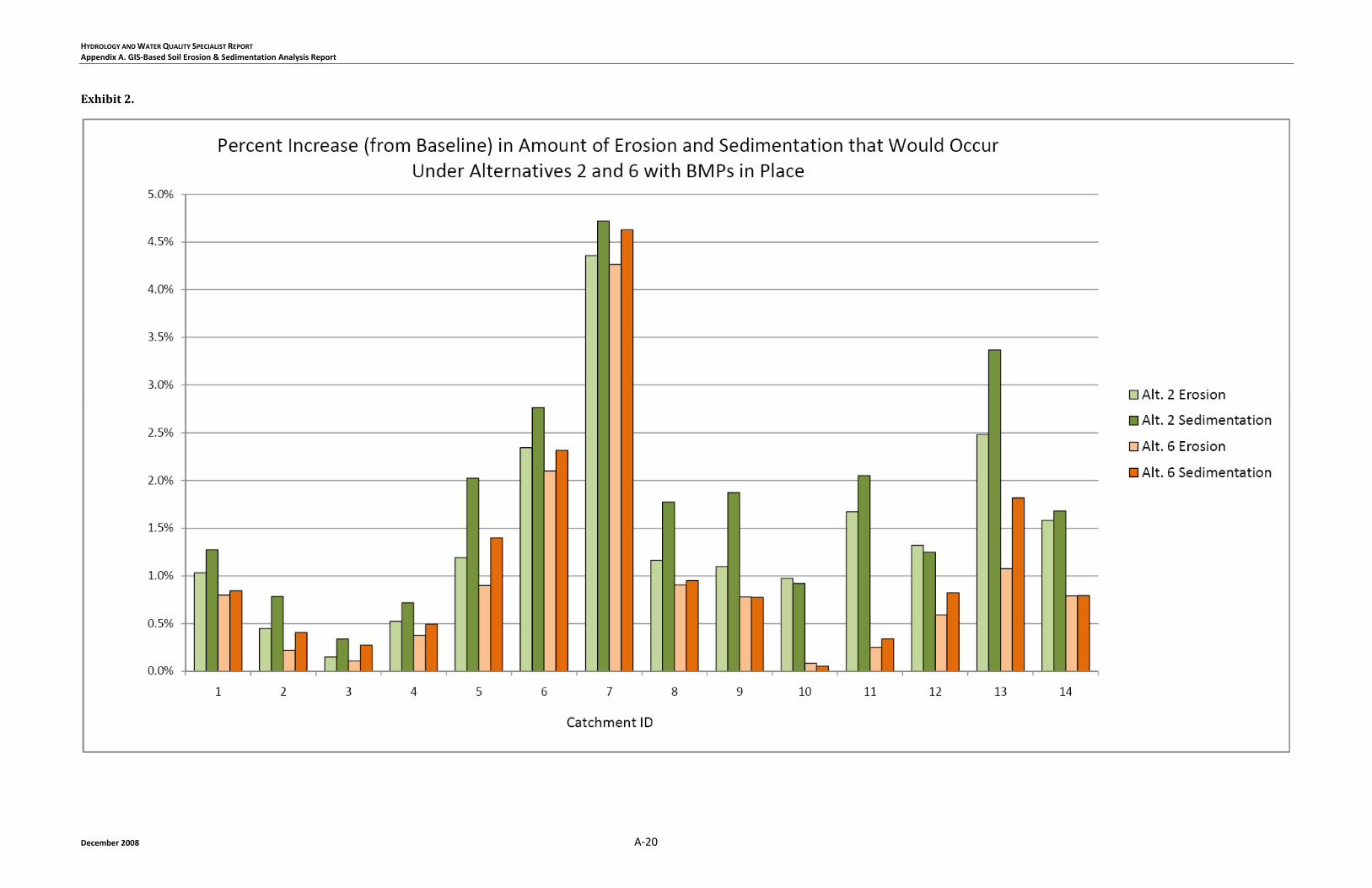
Exhibit 1 (Comparison of Annual Sediment Delivery at Catchment Outlets in the Angeles National Forest), as presented on the following page, provides a visual representation of the results discussed above. In addition, Exhibit 2 (Percent Increase (from Baseline) in Amount of Erosion and Sedimentation that Would Occur Under Alternatives 2 and 6 with BMPs in Place) provides a visual representation of the percent differences between Alternative 2 and Alternative 6, compared to baseline conditions. In comparison with Exhibit 1, which shows the actual sediment delivery amounts that would occur during Project construction, Exhibit 2 depicts the relative increase in sedimentation from baseline values and, therefore, directly facilitates the identification of catchments within which the application of BMPs and/or the implementation of Alternative 6 would be most effective in reducing overall sediment transport and delivery resulting from Project construction.

A comparison of Exhibits 1 and 2 provides several interesting and useful results. For instance, Exhibit 1 shows that among the fourteen catchment areas modeled for this analysis, Catchments 7 and 13 would experience some of the lowest amounts of Project-related erosion and sedimentation under both Alternative 2 and Alternative 6. However, Exhibit 2 indicates that with construction of either alternative, Catchments 7 and 13 would experience a much greater percentage increase in erosion and sedimentation than any of the other catchments. These results indicate that under baseline conditions, Catchments 7 and 13 are characterized by relatively low amounts of erosion and sedimentation and therefore, the soil-disturbing activities that would occur under Alternatives 2 or 6 would result in a more drastic increase in erosion and sedimentation than would occur in a catchment where existing, baseline conditions are more notable, such as in Catchments 5, 8, 9, or 12 (please see Exhibit 1). The largest percentage increases in erosion and sedimentation occur in Catchments 6, 7, 11, and 13. In general, the catchment areas that experience lower amounts of erosion and sedimentation under baseline conditions (as shown in Exhibit 1) would experience a larger percentage increase in erosion and sedimentation under both Alternative 2 and Alternative 6 (as shown in Exhibit 2).

5. Summary and Recommendations

As discussed in Sections 1 and 2 of this report, this sedimentation analysis for the proposed TRTP was prepared in response to a need for quantitative information regarding the potential effects of Project-related sedimentation on aquatic habitats in the ANF, as identified in the biological resources analysis prepared for the EIR/EIS for this project. Through coordination between Aspen and the Forest Service, it was determined that the most appropriate approach for this analysis would be to conduct a combined Revised Universal Soil Loss (RUSLE) and Spatially-Explicit Sediment Delivery Model (SEDMOD) analysis of Alternative 2 (SCE’s proposed Project) and Alternative 6 (Maximum Helicopter Construction in the ANF). As described in Section 1 (Introduction), this sedimentation analysis did not address other identified Project alternatives because only Alternative 6 differs from Alternative 2 with regard to soil-disturbing activities that would occur within the ANF.



Exhibit 1.

NOTE: Sediment Delivery at Outlet corresponds to the amount of sediment in tons per year that is delivered to each modeling point. This represents total annual erosion minus intra‐watershed deposition. Sediment Delivery at Outlet for Catchments 5 and 12 does not properly account for reservoir effects. Calculation should only be used for comparison among alternatives.



Exhibit 2.



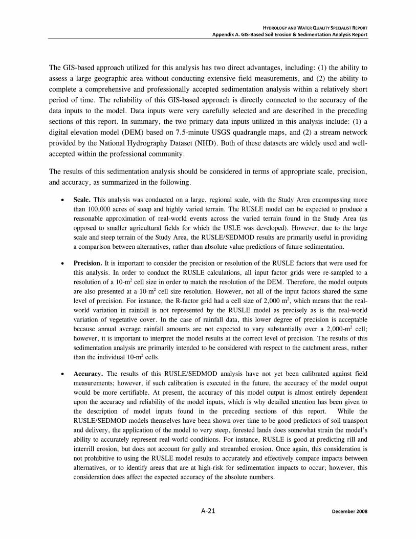
The GIS-based approach utilized for this analysis has two direct advantages, including: (1) the ability to assess a large geographic area without conducting extensive field measurements, and (2) the ability to complete a comprehensive and professionally accepted sedimentation analysis within a relatively short period of time. The reliability of this GIS-based approach is directly connected to the accuracy of the data inputs to the model. Data inputs were very carefully selected and are described in the preceding sections of this report. In summary, the two primary data inputs utilized in this analysis include: (1) a digital elevation model (DEM) based on 7.5-minute USGS quadrangle maps, and (2) a stream network provided by the National Hydrography Dataset (NHD). Both of these datasets are widely used and well-accepted within the professional community.

The results of this sedimentation analysis should be considered in terms of appropriate scale, precision, and accuracy, as summarized in the following.

• Scale. This analysis was conducted on a large, regional scale, with the Study Area encompassing more than 100,000 acres of steep and highly varied terrain. The RUSLE model can be expected to produce a reasonable approximation of real-world events across the varied terrain found in the Study Area (as opposed to smaller agricultural fields for which the USLE was developed). However, due to the large scale and steep terrain of the Study Area, the RUSLE/SEDMOD results are primarily useful in providing a comparison between alternatives, rather than absolute value predictions of future sedimentation.

• Precision. It is important to consider the precision or resolution of the RUSLE factors that were used for this analysis. In order to conduct the RUSLE calculations, all input factor grids were re-sampled to a resolution of a 10-m2 cell size in order to match the resolution of the DEM. Therefore, the model outputs are also presented at a 10-m2 cell size resolution. However, not all of the input factors shared the same level of precision. For instance, the R-factor grid had a cell size of 2,000 m2, which means that the real-world variation in rainfall is not represented by the RUSLE model as precisely as is the real-world variation of vegetative cover. In the case of rainfall data, this lower degree of precision is acceptable because annual average rainfall amounts are not expected to vary substantially over a 2,000-m2 cell; however, it is important to interpret the model results at the correct level of precision. The results of this sedimentation analysis are primarily intended to be considered with respect to the catchment areas, rather than the individual 10-m2 cells.

• Accuracy. The results of this RUSLE/SEDMOD analysis have not yet been calibrated against field measurements; however, if such calibration is executed in the future, the accuracy of the model output would be more certifiable. At present, the accuracy of this model output is almost entirely dependent upon the accuracy and reliability of the model inputs, which is why detailed attention has been given to the description of model inputs found in the preceding sections of this report. While the RUSLE/SEDMOD models themselves have been shown over time to be good predictors of soil transport and delivery, the application of the model to very steep, forested lands does somewhat strain the model’s ability to accurately represent real-world conditions. For instance, RUSLE is good at predicting rill and interrill erosion, but does not account for gully and streambed erosion. Once again, this consideration is not prohibitive to using the RUSLE model results to accurately and effectively compare impacts between alternatives, or to identify areas that are at high-risk for sedimentation impacts to occur; however, this consideration does affect the expected accuracy of the absolute numbers.



As previously mentioned, this GIS-based analysis is particularly useful through its identification of catchment areas in the ANF where the erosion and sedimentation effects of Project-related soil disturbance (under both Alternative 2 and Alternative 6) would be more substantial than other catchment areas. This identification subsequently facilitates the effective implementation of construction BMPs and mitigation measures that will minimize or avoid effects of the Project. Additionally, it is expected that the results of this analysis will be useful for decision-makers in identifying areas where it may be preferable to implement helicopter construction in order to avoid upgrades to certain Forest roads.

It is recommended that mitigation efforts be concentrated on areas of high predicted sedimentation. Although BMPs will be implemented to mitigate the impacts of all Project-related soil-disturbing activities, it is recommended that particular attention be given to monitoring of the effectiveness of BMPs within high-risk Catchments (such as 7 and 13, as described above). Careful monitoring will allow for the timely modification of existing BMPs and/or implementation of additional BMPs, as necessary, and will further reduce the likelihood of any impacts to sensitive aquatic resources.

Although the environmental analysis presented in the EIR/EIS for TRTP does not analyze partial implementation of Alternative 6, it does allow for such a reality by examining both the minimum and maximum helicopter construction scenarios within the ANF. Therefore, environmental effects associated with any combination of Alternative 2 and Alternative 6 are addressed by the current environmental analysis presented in the EIR/EIS. Based on the results the sedimentation analysis, Alternative 6 would be particularly effective in reducing sedimentation within several Catchments. As described above, helicopter construction would provide the greatest reduction in sedimentation compared to Alternative 2 within Catchments 10, 11, 13, and 14, and, conversely, the least reduction in sedimentation compared to Alternative 2 within Catchment 3. This information, in conjunction with the findings of the air quality, biology, noise, and visual resources analyses, can be used to craft the most environmentally protective combination of alternatives in the event that none of the current alternatives is implemented fully.

References

CalWater. 2008. Website: (http://www.ca.nrcs.usda.gov/features/calwater/).

City-Data.com. 2007. “Acton, California.” Website: http://www.city-data.com/city/Acton-California.html. Accessed December 2008.

Dion. 2002. Land development for civil engineers. New York.

Galetovic et al. 1998. Guidelines for the Use of the Revised Universal Soil Loss Equation (RUSLE) Version 1.06 on Mined Lands, Construction Sites, and Reclaimed Lands. Denver: Office of Technology Transfer – Western Regional Coordinating Center of the Office of Surface Mining.

Hickey et al. 1994. Slope length calculations from a DEM with ARC/INFO GRID. Computers, Environment, and Urban Systems, vol. 18, no. 5, pp. 365 – 380.



LADPW, 2005. Los Angeles County Department of Public Works, Water Resources Division. “2004-2005 Hydrologic Report.” Website: http://ladpw.org/wrd/report/0405/index.cfm. Accessed December 2008.

Maidment. 2002. Arc Hydro: GIS for Water Resources. Redlands.

McCool, et al. 1989. Revised slope length factor for the Universal Soil Loss Equation. Transactions of the ASAE, vol. 30, pp. 1387 – 1396.

NLCD, 2006. 2006 National Land Cover Data. Website: http://www.epa.gov/mrlc/nlcd-2006.html. Accessed December 2008.

PRISM Group. 2008. Website: http://www.prism.oregonstate.edu/. Accessed December, 2008.

Rowe, et al. 1949. Probable peak discharges and erosion rates from southern California watersheds as influenced by fire. U.S. Department of Agriculture, Forest Service. California Forest and Range Experiment Station.

SCE (Southern California Edison). 2007. Proponent’s Environmental Assessment, Tehachapi Renewable Transmission Project, (Segments 4 through 11), Southern California Edison Company. June.

Van Remortel, Rick D. 2006. Computation of Soil & Landform Metrics, Version 2. March.

Ibid., 2001. Estimating the LS factor for RUSLE through iterative slope length processing of digital elevation data. Cartography, v. 30, no. 1, pp. 27-35.

Glossary/Acronyms AML: Arc Macro Language

ANF: Angeles National Forest

ArcHydro: GIS program for creating and using data in hydrologic projects.

Baseline: Existing conditions (i.e. the amount / volume of sediment production and delivery that occurs under natural conditions, without the influence of Project activities).

BMP: Best Management Practices

C++: A general computer programming language.

Catchment: Watershed area.

CEQA: California Environmental Quality Act

Deposition: Soils that have eroded as a result of land disturbance but are deposited somewhere within a watershed rather than being transported to a stream channel or a watershed outlet

DEM: Digital elevation model



Discrete Data: Data that can only have certain values; i.e. the opposite of “continuous data”, which can have a wide range of values.

Erosion: The displacement or mobilization of soil; for the purposes of this analysis, “baseline erosion”, or that which occurs naturally as a result of wind, runoff, gravity, etc. is compared to the volume of erosion that would occur as a result of Project-related soil disturbance.

ESRI: Environmental Systems Research Institute, developer of GIS.

Fill: Soils that are digitally added to a depression in the earth.

Floating-Point Data: A representation of continuous data through the use of decimal numbers.

GIS: Geographic Information Systems.

HSA: Hydrologic Sub-Area

HU: Hydrologic Unit

Interrill Erosion: Precipitation causes soil particles to detach, creating shallow overland flows where continued precipitation tends to concentrate and transport additional detached sediment to nearby rill or flow concentration.

IWMC: Interagency Watershed Mapping Committee; in California, the IWMC creates and maintains watershed mapping and dataset information through the CalWater Committee

Orographic: The average height of land, or for a river system, “orographic sequence” represents the proximity of river segments to the source, with the highest-order segment being nearest to the source of the river.

NEPA: National Environmental Policy Act

NFS: National Forest System

NHD: National Hydrography Dataset

NLCD: National Land Cover Dataset

Outflow: The volume of water discharged by a river or stream during a specified period of time.

Overland Flow: A thin film of water flowing over the land surface.

Raster Data: Cell data arranged in a regular grid pattern in which each unit (pixel or cell) in the grid is assigned an identifying value based on its characteristics.

RUSLE: Revised Universal Soil Loss Equation

Sediment delivery: Sedimentation



Sediment transport: Erosion

Sediment yield: Material eroded from land surface that is transported to a stream.

SSURGO: Soil Survey Geographic Database

STATSGO: State Soil Geographic Database

TRTP: Tehachapi Renewable Transmission Project

USGS: United States Geological Society

USLE: Universal Soil Loss Equation

Vector Data: X-Y coordinate representations of locations on the earth that take the form of single points, strings of points (lines or arcs), or closed lines (polygons).

#0#0#0

#0

#0

#0

#0

#0#0

#0

#0#0

#0#0

9 8

7

5 4

1413

121110

6

3

2

1

ANTELOPEHYDROLOGIC UNIT

LOS ANGELES RIVERHYDROLOGIC UNIT

SAN GABRIEL RIVERHYDROLOGIC UNIT

SANTA CLARA - CALLEGUASHYDROLOGIC UNIT

Mill Cree

k

Big Tujunga Creek

Fox C

reek

West Fork San Gabriel River

Alder

Cree

k

Fall Creek

Clear Creek

Chilao C

reek

Trail Fork

Midd

le Fo

rk Mi

ll Cree

k

Lucas Creek

Mule ForkGrott

o Cree

k

Rush

Cree

k

West Fork Alder Creek

North

Fork

Alder

Cree

k

Santa Clara River

Josephine Creek

#0 Catchment OutletNHD StreamsReservoirCatchment Boundaries

AspenEnvironmental Group

1 0 1 20.5 MilesIScale 1:100,000

December 2008

Figure A-1Catchment Outlets for ANF

Sedimentation Modeling

#0

#0

#0

#0

9 8

7

1413

6LOS ANGELES RIVERHYDROLOGIC UNIT


Mill Creek

North Fork Mill Creek

Fall Creek

Midd

le Fo

rk Mi

ll Cree

k

Fox Creek

Santa Clara River

Alder

Cree

k

North Fork Alder Creek

#0 Catchment OutletSoil DisturbanceNHD StreamsReservoirCatchment Boundaries


0.4 0 0.4 0.80.2 MilesIScale 1:100,000

December 2008

Figure A-2Soil Disturbance within the Santa Clara-Calleguas

Hydrologic Unit under the Proposed Project

#0

#0#0

#0

#0

#0

#0

#0#0

#0

#0

#0


9 8

7

5 4

121110

6

3

2

1




Mill Creek

Big Tujunga Creek

Fox Creek

Alder

Cree

k

Fall Creek

Clear Creek


Chilao

Cree

k

Trail Fork

Lucas Creek

Mule Fork

Monte Cristo Creek

East Fork Alder Creek


Grott

o Cree

k

West

Fork

Fox C

reek


Josephine Creek



0.5 0 0.5 10.25 Miles

IScale 1:70,000December 2008

Figure A-3Soil Disturbance within the Los Angeles RiverHydrologic Unit under the Proposed Project

#0

#0#0

#0

#0

#0

#0#0

#0

#0

#0


9 84

121110

3

2



Big Tujunga Creek


Alder

Cree

k

Chilao Creek

Mill Creek

Trail Fork

Lucas Creek Mule Fork East Fork Alder Creek

Grott

o Cree

k

Rush Creek

Fall C

reek

Clear Creek



0.4 0 0.4 0.80.2 Miles


Figure A-4Soil Disturbance within the San Gabriel RiverHydrologic Unit under the Proposed Project

#0

#0

#0

#0

8

7

1413

6




Mill Creek


Fox Creek

Middle Fork M

ill Creek

Fall Creek


Santa Clara River

Alder

Cree

k



0.5 0 0.5 10.25 Miles


Source:

Figure A-5Soil Disturbance within the Santa Clara-Calleguas

Hydrologic Unit under Alternative 6

#0

#0#0

#0

#0

#0

#0

#0#0

#0

#0

#0


9 8

7

5 4

121110

6

3

2

1




Mill Creek

Big Tujunga Creek

Fox Creek

Alder

Cree

k

Fall Creek

Clear Creek


Chilao

Cree

k

Trail Fork

Lucas Creek

Mule Fork

Monte Cristo Creek

East Fork Alder Creek


Grott

o Cree

k

West

Fork

Fox C

reek


Josephine Creek



0.5 0 0.5 10.25 Miles


Figure A-6Soil Disturbance within the Los Angeles River


#0

#0#0

#0

#0

#0

#0#0

#0

#0

#0


9 84

121110

3

2



Big Tujunga Creek


Alder

Cree

k

Chilao Creek

Mill Creek

Trail Fork

Lucas Creek Mule Fork East Fork Alder Creek

Grott

o Cree

k

Rush Creek

Fall C

reek

Clear Creek



0.4 0 0.4 0.80.2 Miles


Figure A-7Soil Disturbance within the San Gabriel River


#0#0#0

#0

#0

#0

#0

#0#0

#0

#0#0

#0#0

9 8

7

5 4

1413

121110

6

3

2

1

Mill Cree

k

Big Tujunga Creek

Fox C

reek


Alder

Cree

k

Fall Creek

Clear Creek

Chilao C

reek

Trail Fork

Midd

le Fo

rk Mi

ll Cree

k

Lucas Creek

Mule ForkGrott

o Cree

k

Rush

Cree

k


North

Fork

Alder

Cree

k

Santa Clara River

Josephine Creek


PRISM-based R-factor valuesValue

High : 298

Low : 6


1 0 1 20.5 MilesIScale 1:100,000

December 2008

Figure A-8PRISM-based R-Factor Grid

at 1-km resolution

#0#0#0

#0

#0

#0

#0

#0#0

#0

#0#0

#0#0

9 8

7

5 4

1413

121110

6

3

2

1

75

58

16

91

Mill Cree

k

Big Tujunga Creek

Fox C

reek


Alder

Cree

k

Fall Creek

Clear Creek

Chilao C

reek

Trail Fork

Midd

le Fo

rk Mi

ll Cree

k

Lucas Creek

Mule ForkGrott

o Cree

k

Rush

Cree

k


North

Fork

Alder

Cree

k

Santa Clara River

Josephine Creek


R-factor values from isoerodent map16587591


1 0 1 20.5 Miles


Figure A-9R-Factor Values estimated at

the Hydrologic Unit scaleusing isoerodent maps

#0#0#0

#0

#0

#0

#0

#0#0

#0

#0#0

#0

#0

9 8

7

5 4

1413

121110

6

3

2

1





Mill Cree

k

Big Tujunga Creek

Fox C

reek


Alder

Cree

k

Fall Creek

Clear Creek

Chilao C

reek

Trail Fork

Midd

le Fo

rk Mi

ll Cree

k

Lucas Creek

Mule ForkGrott

o Cree

k

Rush

Creek


North

Fork

Alder

Cree

k

Santa Clara River

Josephine Creek



1 0 1 20.5 MilesIScale 1:100,000

December 2008

Figure A-10Digital Elevation Model and

Study Area Catchments

#0#0#0

#0

#0

#0

#0

#0#0

#0

#0#0

#0#0

9 8

7

5 4

1413

121110

6

3

2

1





Flow DirectionsNESESSWWNWNE Aspen

Environmental Group1 0 1 20.5 Miles


Figure A-11Flow Direction GRID

based on DEM

#0#0#0

#0

#0

#0

#0

#0#0

#0

#0#0

#0#0

9 8

7

5 4

1413

121110

6

3

2

1





#0 Catchment OutletReservoirCatchment Boundaries


1 0 1 20.5 MilesIScale 1:100,000

December 2008

Figure A-12Flow Accumulation GRID and

Study Area Catchments

#0#0#0

#0

#0

#0

#0

#0#0

#0

#0#0

#0#0

9 8

7

5 4

1413

121110

6

3

2

1





NLCD ClassificationsOpen WaterLow Intensity ResidentialCommercial/Industrial/Trans.Bare Rock/Sand/ClayDeciduous ForestEvergreen ForestMixed ForestShrubland

Orchards/VineyardsGrassland/HerbaceousPasture/HayRow CropsSmall GrainsFallowUrban GrassesWoody Wetlands


1 0 1 20.5 Miles I

Scale 1:100,000December 2008

Figure A-13National Land Cover

Dataset andStudy Area Catchments

#0#0#0

#0

#0

#0

#0

#0#0

#0

#0#0

#0#0

9 8

7

5 4

1413

121110

6

3

2

1





#0 Catchment OutletSoil DisturbanceReservoirCatchment Boundaries

Erosion Risk TAY x 1,000Value

High : 2306430

Low : 0


1 0 1 20.5 Miles


Figure A-14Erosion Risk in Tons/Acre/Year

times 1,000 and SoilDisturbance under the

Proposed Project

#0#0#0

#0

#0

#0

#0

#0#0

#0

#0#0

#0

#0

9 8

7

5 4

1413

121110

6

3

2

1





Mill Cree

k

Big Tujunga Creek

Fox C

reek


Alder

Cree

k

Fall Creek

Clear Creek

Chilao C

reek

Trail Fork

Midd

le Fo

rk Mi

ll Cre

ek

Lucas Creek

Mule ForkGrott

o Cree

k

Rush

Cree

k


North

Fork

Alder

C ree

k

Santa Clara River

Josephine Creek

#0 Catchment OutletSoil DisturbanceReservoirCatchment Boundaries

Erosion Risk TAY x 1.000Value

High : 2070051

Low : 0


1 0 1 20.5 Miles


Figure A-15Erosion Risk in Tons/Acre/Year

times 1,000 and SoilDisturbance under Alternative 6

Documents

Appendix A. GIS-Based Soil Erosion and Sedimentation