Appendix A Linear Algebra for Quantum Computation3A978-3-319...Appendix A: Linear Algebra for Quantum Computation 249 Two vectors v 1 and v 2 are orthogonal if the inner product (v

Appendix ALinear Algebra for Quantum Computation

The goal of this appendix is to compile the definitions, notations, and facts of linearalgebra that are important for this book. Quantum computation has inherited linearalgebra from quantum mechanics as the supporting language for describing thisarea. It is essential to have a solid knowledge of the basic results of linear algebrato understand quantum computation and quantum algorithms. If the reader does nothave this base knowledge, we suggest reading some basic references recommendedat the end of this appendix.

A.1 Vector Spaces

A vector space V over the field of complex numbersC is a nonempty set of elementscalled vectors together with two operations called vector addition and multiplicationof a vector by a scalar in C. The addition operation is associative and commutativeand satisfies the following axioms:

• There is an element 0 ∈ V , such that, for each v ∈ V , v + 0 = 0 + v = v (exis-tence of neutral element).

• For each v ∈ V , there exists u = (−1)v in V such that v + u = 0 (existence ofinverse element).

0 is called zero vector. The scalar multiplication operation satisfies the followingaxioms:

• a.(b.v) = (a.b).v (associativity),• 1.v = v (1 is the neutral element of multiplication),• (a + b).v = a.v + b.v (distributivity over sum of scalars),• a.(v + w) = a.v + a.w (distributivity over vector addition).

where v, w ∈ V and a, b ∈ C.A vector space can be infinite, but in most applications in quantum computation,

finite vector spaces are used and are denoted by Cn , where n is the number of

© Springer Nature Switzerland AG 2018R. Portugal, Quantum Walks and Search Algorithms, Quantum Scienceand Technology, https://doi.org/10.1007/978-3-319-97813-0

247

248 Appendix A: Linear Algebra for Quantum Computation

dimensions. In this case, the vectors have n complex entries. In this book, we rarelyuse infinite spaces, and in these few cases, we are interested only in finite subspaces.In the context of quantum mechanics, infinite vector spaces are used more frequentlythan finite spaces.

A basis for Cn consists of exactly n linearly independent vectors. If {v1, . . . , vn}is a basis for Cn , then an arbitrary vector v can be written as

v =n∑

i=1

aivi ,

where coefficients ai are complex numbers. The dimension of a vector space is thenumber of basis vectors and is denoted by dim(V ).

A.2 Inner Product

The inner product is a binary operation (·, ·) : V × V �→ C, which obeys the fol-lowing properties:

1. (·, ·) is linear in the second argument

(v,

n∑

i=1

aivi

)=

n∑

i=1

ai (v, vi ) .

2. (v1, v2) = (v2, v1)∗.

3. (v, v) ≥ 0. The equality holds if and only if v = 0.

In general, the inner product is not linear in the first argument. The property inquestion is called conjugate-linear.

There is more than one way to define an inner product on a vector space. In Cn ,

the most used inner product is defined as follows: If

v =⎡

⎢⎣a1...

an

⎤

⎥⎦ , w =⎡

⎢⎣b1...

bn

⎤

⎥⎦ ,

then

(v, w) =n∑

i=1

a∗i bi .

This expression is equivalent to the matrix product of the transpose–conjugate vectorv† and w.

Appendix A: Linear Algebra for Quantum Computation 249

Two vectors v1 and v2 are orthogonal if the inner product (v1, v2) is zero. Wealso introduce the notion of norm using the inner product. The norm of v, denotedby ‖v‖, is defined as

‖v‖ = √(v, v).

A normalized vector or unit vector is a vector whose norm is equal to 1. A basis issaid orthonormal if all vectors are normalized and mutually orthogonal.

A finite vector space with an inner product is called a Hilbert space and denotedbyH. In order to an infinite vector space be a Hilbert space, it must obey additionalproperties besides having an inner product. Since we deal primarily with finite vectorspaces, we use the term Hilbert space as a synonym for vector space with an innerproduct. A vector subspace (or simply subspace) W of a finite Hilbert space V isalso a Hilbert space. The set of vectors orthogonal to all vectors of W is the Hilbertspace W⊥ called orthogonal complement. V is the direct sum of W and W⊥, thatis, V = W ⊕ W⊥. A N -dimensional Hilbert space is denoted byHN to highlight itsdimension. A Hilbert space associated with a system A is denoted byHA or simplyA. If A is a subspace of H, then H = A + A⊥, which means that any vector in Hcan be written as a sum of a vector in A and a vector in A⊥.

Exercise A.1. LetA andB be subspaces ofH. Show that dim(A + B) = dim(A) +dim(B) − dim(A ∩ B),

(A + B)⊥ = A⊥ ∩ B⊥, and(A ∩ B)⊥ = A⊥ + B⊥.

Exercise A.2. Give one example of subspacesA andB ofC3 such that (A ∩ B)⊥ �=A ∩ B⊥ + A⊥ ∩ B + A⊥ ∩ B⊥.

A.3 The Dirac Notation

In this review of linear algebra, we use the Dirac or bra–ket notation, which wasintroduced by the English physicist Paul Dirac in the context of quantum mechanicsto aid algebraic manipulations. This notation is very easy to grasp. Several alternativenotations for vectors are used, such as v and �v. The Dirac notation uses |v〉. Up to thispoint, instead of using boldface or an arrow over letter v, we put letter v between avertical bar and a right angle bracket. Ifwe have an indexed basis, that is, {v1, . . . , vn},in the Dirac notation we use the form {|v1〉, . . . , |vn〉} or {|1〉, . . . , |n〉}. Note that ifwe are using a single basis, letter v is unnecessary in principle. Computer scientistsusually start counting from 0. So, the first basis vector is usually called v0. In theDirac notation we have

v0 = |0〉.

Vector |0〉 is not the zero vector; it is only the first vector in a collection of vectors.The zero vector is an exception, whose notation is not modified. Here we use thenotation 0.

Suppose that vector |v〉 has the following entries in a basis


|v〉 =⎡

⎢⎣a1...

an

⎤

⎥⎦ .

The dual vector is denoted by 〈v| and is defined by

〈v| = [a∗1 · · · a∗

n

].

Vectors and their duals can be seen as column and row matrices, respectively. Thematrix product of 〈v| and |v〉, denoted by

⟨v∣∣v⟩, is

⟨v∣∣v⟩ =

n∑

i=1

a∗i ai ,

which coincides with (|v〉, |v〉). Then, the norm of a vector in the Dirac notation is

∥∥|v〉∥∥ =√⟨

v∣∣v⟩.

If {|v1〉, . . . , |vn〉} is an orthonormal basis, then

⟨vi∣∣v j⟩ = δi j ,

where δi j is the Kronecker delta. We use the terminology ket for the vector |v〉 andbra for the dual vector 〈v|. Keeping consistency, we use the terminology bra–ket for⟨v∣∣v⟩.

It is also very common to see the matrix product of |v〉 and 〈v|, denoted by |v〉〈v|,known as the outer product, whose result is a n × n matrix

|v〉〈v| =⎡

⎢⎣a1...

an

⎤

⎥⎦ · [a∗1 · · · a∗

n

]

=⎡

⎢⎣a1a∗

1 · · · a1a∗n

. . .

ana∗1 · · · ana∗

n

⎤

⎥⎦ .

The key to the Dirac notation is to always view kets as column matrices, bras asrow matrices, and recognize that a sequence of bras and kets is a matrix product,hence associative, but noncommutative.


A.4 Computational Basis

The computational basis of Cn is {|0〉, . . . , |n − 1〉}, where

|0〉 =

⎡

⎢⎢⎢⎣

10...

0

⎤

⎥⎥⎥⎦ , . . . , |n − 1〉 =

⎡

⎢⎢⎢⎣

00...

1

⎤

⎥⎥⎥⎦ .

This basis is also known as canonical basis. A few times we use the numberingof the computational basis beginning with |1〉 and ending with |n〉. In this book,when we use a small-caption Latin letter within a ket or bra, we are referring to thecomputational basis. Then, the following expression is always valid

⟨i∣∣ j⟩ = δi j .

The normalized sum of all computational basis vectors defines vector

|D〉 = 1√n

n−1∑

i=0

|i〉,

which we call diagonal state. When n = 2, the diagonal state is given by |D〉 = |+〉,where

|+〉 = |0〉 + |1〉√2

.

Exercise A.3. Calculate explicitly the values of |i〉〈 j | andn−1∑

i=0

|i〉〈i |

in C3.

A.5 Qubit and the Bloch Sphere

The qubit is a unit vector in vector space C2. An arbitrary qubit |ψ〉 is representedby

|ψ〉 = α |0〉 + β |1〉,

where coefficients α and β are complex numbers and obey the constraint


Fig. A.1 Bloch sphere. Thestate |ψ〉 of a qubit isrepresented by a point on thesphere

θ

φ

|ψ〉

x

y

z|0〉

|1〉

|α|2 + |β|2 = 1.

The set {|0〉, |1〉} is the computational basis of C2, and α, β are called amplitudesof state |ψ〉. The term state (or state vector) is used as a synonym for unit vector ina Hilbert space.

In principle, we need four real numbers to describe a qubit, two for α and two forβ. The constraint |α|2 + |β|2 = 1 reduces to three numbers. In quantum mechanics,two vectors that differ from a global phase factor are considered equivalent. Aglobal phase factor is a complex number of unit modulus multiplying the state. Byeliminating this factor, a qubit can be described by two real numbers θ and φ asfollows:

|ψ〉 = cosθ

2|0〉 + eiφ sin

θ

2|1〉,

where 0 ≤ θ ≤ π and 0 ≤ φ < 2π . In the notation above, state |ψ〉 can be rep-resented by a point on the surface of a sphere of unit radius called Bloch sphere.Numbers θ and φ are spherical angles that locate the point that describes |ψ〉, asshown in Fig. A.1. The vector showed there is given by

⎡

⎣sin θ cosφ

sin θ sin φ

cos θ

⎤

⎦ .

When we disregard global phase factors, there is a one-to-one correspondencebetween the quantum states of a qubit and the points on the Bloch sphere. State |0〉is the north pole of the sphere because it is obtained by taking θ = 0. State |1〉 is thesouth pole. States

|±〉 = |0〉 ± |1〉√2


are the intersection points of the x-axis and the sphere; states (|0〉 ± i|1〉)/√2 arethe intersection points of the y-axis with the sphere.

The representation of classical bits in this context is given by the poles of theBloch sphere, and the representation of the probabilistic classical bit, that is, 0 withprobability p and 1 with probability 1 − p, is given by the point on z-axis withcoordinate 2p − 1. The interior of the Bloch sphere is used to describe states of aqubit in the presence of decoherence.

Exercise A.4. Using the Dirac notation, show that opposite points on the Blochsphere correspond to orthogonal states.

Exercise A.5. Suppose you know that the state of a qubit is either |+〉 with proba-bility p or |−〉 with probability 1 − p. If this is the best you know about the state ofthe qubit, where on the Bloch sphere would you represent this qubit?

A.6 Linear Operators

Let V and W be vector spaces, {|v1〉, . . . , |vn〉} a basis for V , and A a functionA : V �→ W that satisfies

A(∑

i

ai |vi 〉)

=∑

i

aiA(|vi 〉),

for any complex numbers ai . A is called a linear operator from V to W . Theterm linear operator on V means that both the domain and codomain of A areV . The composition of linear operators A : V1 �→ V2 and B : V2 �→ V3 is also alinear operator C : V1 �→ V3 obtained through the composition of their functions:C(|v〉) = B(A(|v〉)). The sum of two linear operators, both from V to W , is definedby formula (A + B)(|v〉) = A(|v〉) + B(|v〉).

The identity operator I on V is a linear operator such that I(|v〉) = |v〉 for all|v〉 ∈ V . The null operator O on V is a linear operator such that O(|v〉) = 0 for all|v〉 ∈ V .

The rank of a linear operator A on V is the dimension of the image of A. Thekernel or nullspace or support of a linear operator A on V is the set of all vectors|v〉 such that A(|v〉) = 0. The dimension of the kernel is called the nullity of theoperator. The rank–nullity theorem states that rank(A) + nullity(A) = dim(V ).

Fact

If we specify the action of a linear operatorA on a basis of vector space V , the actionof A on any vector in V can be determined by using the linearity property.


A.7 Matrix Representation

Linear operators are represented by matrices. Let A : V �→ W be a linear operator.Let {|v1〉, . . . , |vn〉} and {|w1〉, . . . , |wm〉} be orthonormal bases for V and W , re-spectively. Thematrix representation ofA is obtained by applyingA to every vectorin the basis of V and expressing the result as a linear combination of basis vectorsof W , as follows:

A (∣∣v j⟩) =

m∑

i=1

ai j |wi 〉,

where index j run from 1 to n. Therefore, ai j are entries of am × n matrix, which wecall A. In this case, expressionA (∣∣v j

⟩), whichmeans functionA applied to argument∣∣v j

⟩, is equivalent to the matrix product A

∣∣v j⟩. Using the outer product notation, we

have

A =m∑

i=1

n∑

j=1

ai j |wi 〉⟨v j

∣∣.

Using the above equation and the fact that the basis of V is orthonormal, we canverify that the matrix product of A and

∣∣v j⟩is equal to A (∣∣v j

⟩). The key to this

calculation is to use the associativity of matrix multiplication:

(|wi 〉⟨v j

∣∣)|vk〉 = |wi 〉( ⟨

v j

∣∣vk⟩ )

= δ jk |wi 〉.

In particular, the matrix representation of the identity operator I in any orthonor-mal basis is the identity matrix I and the matrix representation of the null operatorO in any orthonormal basis is the zero matrix.

If the linear operator C is the composition of the linear operators B and A, thematrix representation of C is obtained by multiplying the matrix representation of Bwith that of A, that is, C = BA.

When we fix orthonormal bases for the vector spaces, there is a one-to-one corre-spondence between linear operators and matrices. In C

n , we use the computationalbasis as a reference basis, so that the terms linear operator and matrix are taken assynonyms. We also use the term operator as a synonym for linear operator.

Exercise A.6. Suppose B is an operator whose action on the computational basisof the n-dimensional vector space V is

B| j〉 = ∣∣ψ j⟩,

where∣∣ψ j⟩are vectors in V for all j .

1. Obtain the expression of B using the outer product.2. Show that

∣∣ψ j⟩is the j th column in the matrix representation of B.


3. Suppose that B is the Hadamard operator

H = 1√2

[1 11 −1

].

Redo the previous items using operator H .

A.8 Diagonal Representation

Let A be an operator on V . If there exists an orthonormal basis {|v1〉, . . . , |vn〉} of Vsuch that

A =n∑

i=1

λi |vi 〉〈vi |,

we say that A admits a diagonal representation or, equivalently, A is diagonalizable.The complex numbers λi are the eigenvalues of A and |vi 〉 are the correspondingeigenvectors. A vector |ψ〉 is an eigenvector of A if there is a scalar λ, called eigen-value, so that

A|ψ〉 = λ|ψ〉.

Any multiple of an eigenvector is also an eigenvector. If two eigenvectors are asso-ciated with the same eigenvalue, then any linear combination of these eigenvectorsis an eigenvector. The number of linearly independent eigenvectors associated withthe same eigenvalue is the multiplicity of that eigenvalue. We use the short notation“λ-eigenvectors” for eigenvectors associated with eigenvalues λ.

If there are eigenvalues with multiplicity greater than one, the diagonal represen-tation is factored out as follows:

A =∑

λ

λPλ,

where index λ runs only on the distinct eigenvalues and Pλ is the projector onthe eigenspace of A associated with eigenvalue λ. If λ has multiplicity 1, Pλ =|v〉〈v|, where |v〉 is the unit eigenvector associated with λ. If λ has multiplic-ity 2 and |v1〉, |v2〉 are linearly independent unit eigenvectors associated with λ,Pλ = |v1〉〈v1| + |v2〉〈v2| and so on. The projectors Pλ satisfy

∑

λ

Pλ = I.

An alternative way to define a diagonalizable operator is by requiring that A issimilar to a diagonal matrix.Matrices A and A′ are similar if A′ = M−1AM for someinvertible matrix M . We have interest only in the case when M is a unitary matrix.


The term diagonalizable used here is narrower than the one used in the literaturebecause we are demanding that M be a unitary matrix.

The characteristic polynomial of a matrix A, denoted by pA(λ), is the monicpolynomial

pA(λ) = det(λI − A).

The roots of pA(λ) are the eigenvalues of A. Usually, the best way to calculate theeigenvalues of a matrix is via the characteristic polynomial. For a two-dimensionalmatrix U , the characteristic polynomial is given by

pU (λ) = λ2 − tr(U ) λ + det(U ).

IfU is a real unitary matrix, the eigenvalues have the form e±iω and the characteristicpolynomial is given by

pU (λ) = λ2 − 2λ cosω + 1.

Exercise A.7. Suppose that A is a diagonalizable operator with eigenvalues ±1.Show that

P±1 = I ± A

2.

A.9 Completeness Relation

The completeness relation is so useful that it deserves to be highlighted. Let {|v1〉, . . .,|vn〉} be an orthonormal basis of V . Then,

I =n∑

i=1

|vi 〉〈vi |.

The completeness relation is the diagonal representation of the identity matrix.

Exercise A.8. If {|v1〉, . . . , |vn〉} is an orthonormal basis, it is straightforward toshow that

A =m∑

i=1

n∑

j=1

ai j |wi 〉⟨v j

∣∣

implies

A∣∣v j⟩ =

m∑

i=1

ai j |wi 〉.

Prove the reverse, that is, given the above expressions for A∣∣v j⟩, use the completeness

relation to obtain A. [Hint: Multiply the last equation by⟨v j

∣∣ and sum over j .]


A.10 Cauchy–Schwarz Inequality

Let V be a Hilbert space and |v〉, |w〉 ∈ V . Then,

∣∣ ⟨v∣∣w⟩ ∣∣ ≤

√⟨v∣∣v⟩ ⟨

w∣∣w⟩.

A more explicit way of presenting the Cauchy–Schwarz inequality is

∣∣∣∣∣∑

i

viwi

∣∣∣∣∣

2

≤(∑

i

|vi |2)(∑

i

|wi |2)

,

which is obtained when we take |v〉 =∑i v∗i |i〉 and |w〉 =∑i wi |i〉.

A.11 Special Operators

Let A be a linear operator on Hilbert space V . Then, there exists a unique linearoperator A† on V , called adjoint operator, that satisfies

(|v〉, A|w〉) = (A†|v〉, |w〉) ,

for all |v〉, |w〉 ∈ V .The matrix representation of A† is the transpose–conjugate matrix (A∗)T . The

main properties of the dagger or transpose–conjugate operation are

1. (A B)† = B†A†

2. |v〉† = 〈v|3.(A|v〉)† = 〈v|A†

4.(|w〉〈v|)† = |v〉〈w|

5.(A†)† = A

6.(∑

i ai Ai)† =∑i a

∗i A

†i

The last property shows that the dagger operation is conjugate-linear when appliedon a linear combination of operators.

Normal Operator

An operator A on V is normal if A†A = AA†.

Spectral Theorem

An operator A on V is diagonalizable if and only if A is normal.

Unitary Operator

An operator U on V is unitary if U †U = UU † = I .


Facts about Unitary Operators

Unitary operators are normal. They are diagonalizable with respect to an orthonormalbasis. Eigenvectors of a unitary operator associated with different eigenvalues areorthogonal. The eigenvalues have unit modulus, that is, they have the form eiα , whereα is a real number . Unitary operators preserve the inner product, that is, the innerproduct ofU |v1〉 andU |v2〉 is equal to the inner product of |v1〉 and |v2〉. The actionof a unitary operator on a vector preserves its norm.

Hermitian Operator

An operator A on V is Hermitian or self-adjoint if A† = A.

Facts about Hermitian Operators

Hermitian operators are normal. They are diagonalizable with respect to an orthonor-mal basis. Eigenvectors of a Hermitian operator associated with different eigenvaluesare orthogonal. The eigenvalues of a Hermitian operator are real numbers. A realsymmetric matrix is Hermitian.

Orthogonal Projector

An operator P on V is an orthogonal projector if P2 = P and P† = P .

Facts about Orthogonal Projectors

The eigenvalues are equal to 0 or 1. If P is an orthogonal projector, then the orthog-onal complement I − P is also an orthogonal projector. Applying a projector to avector either decreases its norm or maintains invariant. In this book, we use the termprojector as a synonym for orthogonal projector. We use the term nonorthogonalprojector explicitly to distinguish this case. An example of a nonorthogonal projectoron a qubit is P = |1〉(〈0| + 〈1|). Note that P is not normal in this example.

Positive Operator

An operator A on V is said positive if⟨v∣∣A∣∣v⟩ ≥ 0 for any |v〉 ∈ V . If the inequality

is strict for any nonzero vector in V , then the operator is said positive definite.

Facts about Positive Operators

Positive operators are Hermitian. The eigenvalues are nonnegative real numbers.

Exercise A.9. Consider matrix

M =[1 0

1 1

].

1. Show that M is not normal.2. Show that the eigenvectors of M generate a one-dimensional space.


Exercise A.10. Consider matrix

M =[1 0

1 −1

].

1. Show that the eigenvalues of M are ±1.2. Show that M is not unitary nor Hermitian.3. Show that the eigenvectors associated with distinct eigenvalues of M are not

orthogonal.4. Show that M has a diagonal representation.

Exercise A.11. 1. Show that the product of two unitary operators is a unitaryoperator.

2. The sum of two unitary operators is necessarily a unitary operator? If not, givea counterexample.

Exercise A.12. 1. Show that the sum of two Hermitian operators is a Hermitianoperator.

2. The product of two Hermitian operators is necessarily a Hermitian operator? Ifnot, give a counterexample.

Exercise A.13. Show that A†A is a positive operator for any operator A.

A.12 Pauli Matrices

The Pauli matrices are

σ0 = I =[1 00 1

],

σ1 = σx = X =[0 11 0

],

σ2 = σy = Y =[0 −ii 0

],

σ3 = σz = Z =[1 00 −1

].

These matrices are unitary and Hermitian, and hence their eigenvalues are equal to±1. Putting in another way: σ 2

j = I and σ†j = σ j to j = 0, . . . , 3.

The following facts are extensively used:

X |0〉 = |1〉, X |1〉 = |0〉,


Z |0〉 = |0〉, Z |1〉 = −|1〉.

Pauli matrices form a basis for the vector space of 2 × 2 matrices. Therefore, anarbitrary operator that acts on a qubit can be written as a linear combination of Paulimatrices.

Exercise A.14. Consider the representation of the state |ψ〉 of a qubit on the Blochsphere. What is the representation of states X |ψ〉, Y |ψ〉, and Z |ψ〉 relative to |ψ〉?What is the geometric interpretation of the action of the Pauli matrices on the Blochsphere?

A.13 Operator Functions

If we have an operator A on V , we ask whether it is possible to calculate√A, that

is, to find an operator whose square is A? It is more interesting to ask ourselveswhether it makes sense to use an operator as an argument of an arbitrary functionf : C �→ C, such as the exponential or logarithmic function. If f is analytic, we usethe Taylor expansion of f (x) and replace x by A. This will not work for the squareroot function. There is an alternate route for lifting f if operator A is normal. Usingthe diagonal representation, A can be written in the form

A =∑

i

ai |vi 〉〈vi |,

where ai are the eigenvalues and the set {|vi 〉} is an orthonormal basis of eigenvec-tors of A. We extend the application of a function f : C �→ C to the set of normaloperators as follows. If A is a normal operator, then

f (A) =∑

i

f (ai )|vi 〉〈vi |.

The result is an operator defined on the same vector space V .If the goal is to calculate

√A, first A must be diagonalized, that is, we must

determine a unitary matrix U such that A = UDU †, where D is a diagonal matrix.Then, we use the fact that

√A = U

√DU †, where

√D is calculated by taking the

square root of each diagonal element.IfU is the evolution operator of an isolated quantum systemwhose state is |ψ(0)〉

initially, the state at time t is given by

|ψ(t)〉 = Ut |ψ(0)〉.

Usually, the most efficient way to calculate state |ψ(t)〉 is to obtain the diagonalrepresentation of the unitary operator U , described as


U =∑

i

λi |vi 〉〈vi |,

and to calculate the t th power of U , which is

Ut =∑

i

λti |vi 〉〈vi |.

The system state at time t will be

|ψ(t)〉 =∑

i

λti

⟨vi∣∣ψ(0)

⟩ |vi 〉.

The trace of a matrix is another type of operator function. In this case, the resultof applying the trace function is a complex number defined as

tr(A) =∑

i

aii ,

where aii is the i th diagonal element of A. In the Dirac notation,

tr(A) =∑

i

〈vi |A|vi 〉,

where {|v1〉, . . . , |vn〉} is an orthonormal basis of V . The trace function satisfies thefollowing properties:

1. (Linearity) tr(aA + bB) = a tr(A) + b tr(B),

2. (Commutativity) tr(AB) = tr(BA),

3. (Cyclic property) tr(A B C) = tr(CA B).

The third property follows from the second one. Properties 2 and 3 are valid when A,B, and C are not square matrices (AB, ABC , and CAB must be square matrices).

The trace function is invariant under the similarity transformation, that is,tr(M−1AM) = tr(A), where M is an invertible matrix. This implies that the tracedoes not depend on the basis choice for the matrix representation of A.

A useful formula involving the trace of operators is

tr(A|ψ〉〈ψ |) = ⟨ψ∣∣A∣∣ψ ⟩ ,

for any |ψ〉 ∈ V and any A on V . This formula is easily proved using the cyclicproperty of the trace function.

Exercise A.15. Using the method of applying functions to matrices described inthis section, find all matrices M such that


M2 =[5 4

4 5

].

Exercise A.16. If f is analytic and A is normal, show that f (A) using the Taylorexpansion is equal to f (A) using the spectral decomposition.

A.14 Norm of a Linear Operator

Given a vector space V over the complex numbers, a norm on V is a function‖ ‖ : V → R with the following properties:

• ‖a|ψ〉‖ = |a| ‖|ψ〉‖,• ‖|ψ〉 + ∣∣ψ ′⟩‖ ≤ ‖|ψ〉‖ + ‖∣∣ψ ′⟩‖,• ‖|ψ〉‖ ≥ 0,• ‖|ψ〉‖ = 0 if and only if |ψ〉 = 0,

for all a ∈ C and all |ψ〉, ∣∣ψ ′⟩ ∈ V ,The set of all linear operators on a Hilbert spaceH is a vector space over the com-

plex numbers because it obeys the properties demanded by the definition describedin Sect. A.1. It is possible to define more than one norm on a vector space, and letus start with the following norm.

Let A be a linear operator on a Hilbert space H. The norm of A is defined as

‖A‖ = max⟨ψ

∣∣ψ⟩=1

∣∣⟨ψ∣∣A∣∣ψ⟩∣∣ ,

where the maximum is over all normalized states |ψ〉 ∈ H.The next norm is induced from an inner product. The Hilbert–Schmidt inner

product (also known as Frobenius inner product) of two linear operators A and B is

(A, B) = tr(A†B

).

Now, we can define another norm (trace norm) of a linear operator A on a Hilbertspace H as

‖A‖tr =√tr(A†A

).

In a normed vector space, the distance between vectors |ψ〉 and ∣∣ψ ′⟩ is given by‖|ψ〉 − ∣∣ψ ′⟩‖. Then, it makes sense to speak about distance between linear operatorsA and B, which is the nonnegative number ‖A − B‖.Exercise A.17. Show that ‖U‖ = 1 if U is a unitary operator.

Exercise A.18. Show that the inner product (A, B) = tr(A†B) satisfies the proper-ties described in Sect. A.2.


Exercise A.19. Show that ‖U‖tr = √n if U is a unitary operator on Cn .

Exercise A.20. Show that both norms defined in this section satisfy the propertiesdescribed at the beginning of this section.

A.15 Tensor Product

Let V and W be finite Hilbert spaces with basis {|v1〉, . . ., |vm〉} and {|w1〉, . . .,|wn〉}, respectively. The tensor product of V and W , denoted by V ⊗ W , is a (mn)-dimensional Hilbert space with basis {|v1〉 ⊗ |w1〉, |v1〉 ⊗ |w2〉, . . . , |vm〉 ⊗ |wn〉}.The tensor product of a vector in V and a vector in W , such as |v〉 ⊗ |w〉, alsodenoted by |v〉|w〉 or |v,w〉 or |v w〉, is calculated explicitly via the Kroneckerproduct, defined ahead. An arbitrary vector in V ⊗ W is a linear combination ofvectors |vi 〉 ⊗ ∣∣w j

⟩, that is, if |ψ〉 ∈ V ⊗ W , then

|ψ〉 =m∑

i=1

n∑

j=1

ai j |vi 〉 ⊗ ∣∣w j⟩.

The tensor product is bilinear, that is, linear with respect to each argument:

1. |v〉 ⊗ (a |w1〉 + b |w2〉) = a |v〉 ⊗ |w1〉 + b |v〉 ⊗ |w2〉,

2.(a |v1〉 + b |v2〉

)⊗ |w〉 = a |v1〉 ⊗ |w〉 + b |v2〉 ⊗ |w〉.A scalar can always be factored out to the beginning of the expression:

a(|v〉 ⊗ |w〉) = (

a|v〉)⊗ |w〉 = |v〉 ⊗ (a|w〉).

The tensor product of a linear operator A on V and B on W , denoted by A ⊗ B,is a linear operator on V ⊗ W defined by

(A ⊗ B

)(|v〉 ⊗ |w〉) = (A|v〉)⊗ (B|w〉).

In general, an arbitrary linear operator on V ⊗ W cannot be factored out as thetensor product of the form A ⊗ B, but it can be written as a linear combination ofoperators of the form Ai ⊗ Bj . The above definition is easily extended to operatorsA : V �→ V ′ and B : W �→ W ′. In this case, the tensor product of these operators is(A ⊗ B) : (V ⊗ W ) �→ (V ′ ⊗ W ′).

In quantum mechanics, it is very common to use operators in the form of externalproducts, for example, A = |v〉〈v| and B = |w〉〈w|. The tensor product of A and Bis represented by the following equivalent ways:


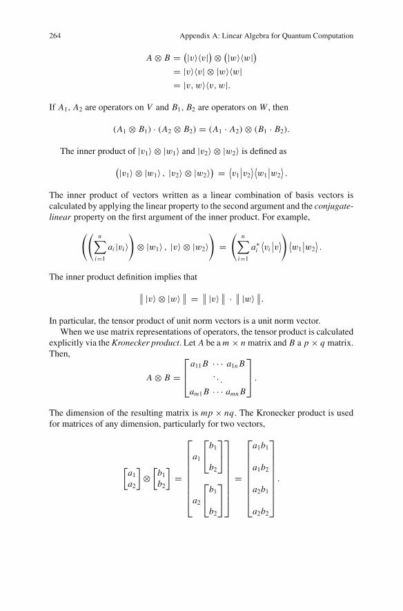
A ⊗ B = (|v〉〈v|)⊗ (|w〉〈w|)= |v〉〈v| ⊗ |w〉〈w|= |v,w〉〈v,w|.

If A1, A2 are operators on V and B1, B2 are operators on W , then

(A1 ⊗ B1) · (A2 ⊗ B2) = (A1 · A2) ⊗ (B1 · B2).

The inner product of |v1〉 ⊗ |w1〉 and |v2〉 ⊗ |w2〉 is defined as

(|v1〉 ⊗ |w1〉 , |v2〉 ⊗ |w2〉) = ⟨

v1∣∣v2⟩ ⟨

w1

∣∣w2⟩.

The inner product of vectors written as a linear combination of basis vectors iscalculated by applying the linear property to the second argument and the conjugate-linear property on the first argument of the inner product. For example,

((n∑

i=1

ai |vi 〉)

⊗ |w1〉 , |v〉 ⊗ |w2〉)

=(

n∑

i=1

a∗i

⟨vi∣∣v⟩)⟨w1

∣∣w2⟩.

The inner product definition implies that

∥∥ |v〉 ⊗ |w〉 ∥∥ = ∥∥ |v〉 ∥∥ · ∥∥ |w〉 ∥∥.

In particular, the tensor product of unit norm vectors is a unit norm vector.When we use matrix representations of operators, the tensor product is calculated

explicitly via the Kronecker product. Let A be am × n matrix and B a p × q matrix.Then,

A ⊗ B =⎡

⎢⎣a11B · · · a1n B

. . .

am1B · · · amn B

⎤

⎥⎦ .

The dimension of the resulting matrix is mp × nq. The Kronecker product is usedfor matrices of any dimension, particularly for two vectors,

[a1a2

]⊗[b1b2

]=

⎡

⎢⎢⎢⎢⎢⎢⎢⎢⎣

a1

⎡

⎣b1

b2

⎤

⎦

a2

⎡

⎣b1

b2

⎤

⎦

⎤

⎥⎥⎥⎥⎥⎥⎥⎥⎦

=

⎡

⎢⎢⎢⎢⎢⎢⎢⎢⎣

a1b1

a1b2

a2b1

a2b2

⎤

⎥⎥⎥⎥⎥⎥⎥⎥⎦

.


The tensor product is an associative and distributive operation, but noncommu-tative, that is, |v〉 ⊗ |w〉 �= |w〉 ⊗ |v〉 if v �= w. Most operations on a tensor productare performed term by term, such as

(A ⊗ B)† = A† ⊗ B†.

If both operators A and B are special operators of the same type, as the ones definedin Sect. A.11, then the tensor product A ⊗ B is also a special operator of the sametype. For example, the tensor product of Hermitian operators is a Hermitian operator.

The trace of a Kronecker product of matrices is

tr(A ⊗ B) = trA trB,

while the determinant is

det(A ⊗ B) = (det A)m (det B)n,

where n is the dimension of A and m of B.If the diagonal state of the vector space V is |D〉V and of space W is |D〉W , then

the diagonal state of space V ⊗ W is |D〉V ⊗ |D〉W . Therefore, the diagonal state ofspace V⊗n is |D〉⊗n , where V⊗n means V ⊗ · · · ⊗ V with n terms.

Exercise A.21. Let H be the Hadamard operator

H = 1√2

[1 11 −1

].

Show that

〈i |H⊗n| j〉 = (−1)i · j√2n

,

where n represents the number of qubits and i · j is the binary inner product, that is,i · j = i1 j1 + · · · + in jn mod 2, where (i1, . . . , in) and ( j1, . . . , jn) are the binarydecompositions of i and j , respectively.

A.16 Quantum Gates, Circuits, and Registers

A quantum circuit is a pictorial way to describe a quantum algorithm. The input lieson the left-hand side of the circuit and the quantum information flows unchangedthrough thewires, from the left to right, until finding aquantumgate, which is a squarebox with the name of a unitary operator. The quantum gate represents the action ofthe unitary operator, which transforms the quantum information and releases it tothe wire on the right-hand side. For example, the algebraic expression |+〉 = H |0〉


is represented by the circuit1

|0〉 H |+〉.

If a measurement is performed, the representation is

|0〉 H

{0,

1.

A meter represents a measurement in the computational basis, and a double wireconveys the classical information that comes out of the meter. In the example, thestate of the qubit right before the measurement is (|0〉 + |1〉)/√2. If the qubit stateis projected on |0〉 after the measurement, the output is 0, otherwise 1.

The controlled NOT gate (CNOT or C(X)) is a 2-qubit gate defined by

CNOT |k〉|�〉 = |k〉Xk |�〉,

and represented by the circuit|k〉 • |k〉|�〉 Xk |�〉.

The qubit marked with the black full point is called control qubit, and the qubitmarked with the ⊕ sign is called the target qubit.

The Toffoli gate C2(X) is a 3-qubit controlled gate defined by

C2(X) | j〉|k〉|�〉 = | j〉|k〉X jk |�〉,

and represented by the circuit| j〉 • | j〉|k〉 • |k〉|�〉 X jk |�〉.

The Toffoli gate has two control qubits and one target qubit.These gates can be generalized. The generalized Toffoli gate Cn(X) is a (n + 1)-

qubit controlled gate defined by

Cn(X) | j1〉...| jn〉| jn+1〉 = | j1〉...| jn〉X j1... jn | jn+1〉.

When defined using the computational basis, the state of the target qubit inverts ifand only if all control qubits are set to one. There is another case in which the stateof the target qubit inverts if and only if all control qubits are set to zero. In this case,the control qubits are depicted by empty controls (empty white points) instead of fullcontrols (full black points), such as

1The circuits were generated with package Q-circuit.


| j〉 | j〉|k〉 |k〉|�〉 X jk |�〉,

whose algebraic representation is

| j1〉| j2〉| j3〉 �−→ | j1〉| j2〉X (1− j1)(1− j2)| j3〉.

It is possible to mix full and empty controls. Those kinds of controlled gates arecalled generalized Toffoli gates.

A register is a set of qubits treated as a composite system. In many quantumalgorithms, the qubits are divided into two registers: one for the main calculationfrom where the result comes out and one for the draft (calculations that will bediscarded).

Suppose we have a register with two qubits. The computational basis is

|0, 0〉 =

⎡

⎢⎢⎣

1000

⎤

⎥⎥⎦ |0, 1〉 =

⎡

⎢⎢⎣

0100

⎤

⎥⎥⎦ |1, 0〉 =

⎡

⎢⎢⎣

0010

⎤

⎥⎥⎦ |1, 1〉 =

⎡

⎢⎢⎣

0001

⎤

⎥⎥⎦ .

An arbitrary state of this register is

|ψ〉 =1∑

i=0

1∑

j=0

ai j |i, j〉

where coefficients ai j are complex numbers that satisfy the constraint

∣∣a00∣∣2 + ∣∣a01

∣∣2 + ∣∣a10∣∣2 + ∣∣a11

∣∣2 = 1.

To help to generalize to n qubits, it is usual to compress the notation by convertingthe base-2 notation to the base-10 notation. The computational basis for a two-qubitregister in the base-10 notation is {|0〉, |1〉, |2〉, |3〉}. In the base-2 notation, we candetermine the number of qubits by counting the number of digits inside the ket; forexample, |011〉 refers to three qubits. In the base-10 notation, we cannot determinewhat is the number of qubits of the register. The number of qubits is implicit. At anypoint, we can go back, write the numbers in the base-2 notation, and the number ofqubits will be clear. In the compact notation, an arbitrary state of a n-qubit registeris

|ψ〉 =2n−1∑

i=0

ai |i〉

where coefficients ai are complex numbers that satisfy the constraint


2n−1∑

i=0

∣∣ai∣∣2 = 1.

The diagonal state of a n-qubit register is the tensor product of the diagonal state ofeach qubit, that is, |D〉 = |+〉⊗n .

A set of universal quantum gates is a finite set of gates that generates any unitaryoperator through tensor and matrix products of gates in the set. Since the number ofpossible quantum gates is uncountable even in the 1-qubit case, we require that anyquantum gate can be approximated by a sequence of universal quantum gates. Onesimple set of universal gates is CNOT, H , X , T (or π/8 gate), and T †, where

T =[1 00 e

iπ4

].

To calculate the time complexity of a quantum algorithm, we have to implement acircuit of the algorithm in terms of universal gates in the best way possible. The timecomplexity is determined by the depth of the circuit.

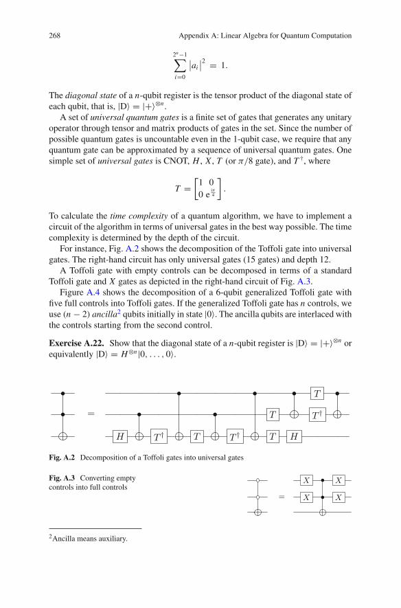
For instance, Fig. A.2 shows the decomposition of the Toffoli gate into universalgates. The right-hand circuit has only universal gates (15 gates) and depth 12.

A Toffoli gate with empty controls can be decomposed in terms of a standardToffoli gate and X gates as depicted in the right-hand circuit of Fig. A.3.

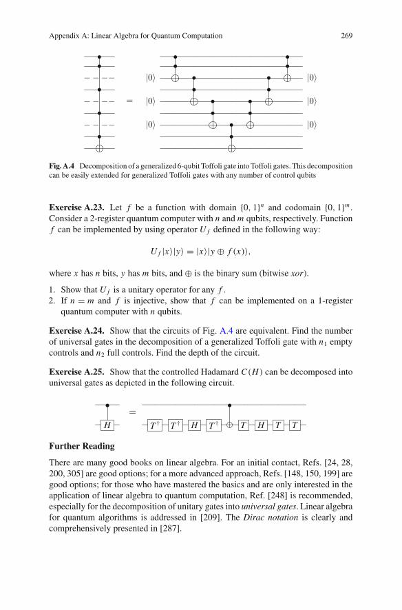
Figure A.4 shows the decomposition of a 6-qubit generalized Toffoli gate withfive full controls into Toffoli gates. If the generalized Toffoli gate has n controls, weuse (n − 2) ancilla2 qubits initially in state |0〉. The ancilla qubits are interlaced withthe controls starting from the second control.

Exercise A.22. Show that the diagonal state of a n-qubit register is |D〉 = |+〉⊗n orequivalently |D〉 = H⊗n|0, . . . , 0〉.

• • • • T •

• = • • T T †

H T † T T † T H

Fig. A.2 Decomposition of a Toffoli gates into universal gates

Fig. A.3 Converting emptycontrols into full controls

X • X

= X • X

2Ancilla means auxiliary.


• • •• • •

− − −− |0〉 • • |0〉• • •

− − −− = |0〉 • • |0〉• • •

− − −− |0〉 • |0〉• •

Fig. A.4 Decomposition of a generalized 6-qubit Toffoli gate intoToffoli gates. This decompositioncan be easily extended for generalized Toffoli gates with any number of control qubits

Exercise A.23. Let f be a function with domain {0, 1}n and codomain {0, 1}m .Consider a 2-register quantum computer with n andm qubits, respectively. Functionf can be implemented by using operator U f defined in the following way:

U f |x〉|y〉 = |x〉|y ⊕ f (x)〉,

where x has n bits, y has m bits, and ⊕ is the binary sum (bitwise xor).

1. Show that U f is a unitary operator for any f .2. If n = m and f is injective, show that f can be implemented on a 1-register

quantum computer with n qubits.

Exercise A.24. Show that the circuits of Fig. A.4 are equivalent. Find the numberof universal gates in the decomposition of a generalized Toffoli gate with n1 emptycontrols and n2 full controls. Find the depth of the circuit.

Exercise A.25. Show that the controlled Hadamard C(H) can be decomposed intouniversal gates as depicted in the following circuit.

• •=H T † T † H T † T H T T

Further Reading

There are many good books on linear algebra. For an initial contact, Refs. [24, 28,200, 305] are good options; for a more advanced approach, Refs. [148, 150, 199] aregood options; for those who have mastered the basics and are only interested in theapplication of linear algebra to quantum computation, Ref. [248] is recommended,especially for the decomposition of unitary gates into universal gates. Linear algebrafor quantum algorithms is addressed in [209]. The Dirac notation is clearly andcomprehensively presented in [287].

Appendix BGraph Theory for Quantum Walks

Graph theory is a large area of mathematics with a wide range of applications,especially in computer science. It is impossible to overstate the importance of graphtheory for quantum walks. In fact, graph theory for quantum walks is as importantas linear algebra for quantum computation.

In the quantum walk setting, the graph represents positions and directions for thewalker’s shift. It is not mandatory to use the graph vertices as the walker’s position.Any interpretation is accepted if it employs the graph structure so that the physicalmeaning reflects the graph components. For example, it makes no sense to have aquantum walk model in which the walker can jump over some vertices, for instance,a model on the line in which the walker can jump from vertex 1 to vertex 3, skippingvertex 2. If it is allowed to jump from vertex 1 to vertex 3, it means that there is anedge or arc linking vertex 1 to vertex 3 and the underlying graph is not the line.

A solid basis on graph theory is required to understand the area of quantum walk.This appendix focuses on the main definitions of graph theory used in this work withsome brief examples and should not be used as the first contact with graph theory.At the end of this appendix, introductory and advanced references for starters andfor further reading are given.

B.1 Basic Definitions

A simple graph (V, E) is defined by a set V ( ) of vertices or nodes and a setE( ) of edges so that each edge links two vertices and two vertices are linked byat most one edge. Two vertices linked by an edge are called adjacent or neighbors.The neighborhood of a vertex v ∈ V , denoted by N (v), is the set of vertices adjacentto v. Two edges that share a common vertex are also called adjacent. A loop is anedge whose endpoints are equal. Multiple edges are edges having the same pair ofendpoints. A simple graph has no loops nor multiple edges. In simple graphs, theedges can be named by the endpoints like an unordered set {v, v′}, where v and v′are vertices.


271

272 Appendix B: Graph Theory for Quantum Walks

The degree of vertex v is the number of edges incident to the vertex and is denotedby d(v). The maximum degree is denoted by �( ), and the minimum degree isdenoted by δ( ). A graph is d-regular if all vertices have degree d, that is, eachvertex has exactly d neighbors. The handshaking lemma states that every graph hasan even number of vertices with odd degree, which is a consequence of the degreesum formula ∑

v∈Vd(v) = 2|E |.

A path is a list v0, e1, v1, . . . , ek , vk of vertices and edges such that edge ei hasendpoints vi−1 and vi . A cycle is a closed path.

Agraph is connectedwhen there is a path between every pair of vertices; otherwiseit is called disconnected. An example of connect graph is the complete graph, whichdenoted by KN where N is the number of vertices, and is a simple graph in whichevery pair of distinct vertices is connected by an edge.

A subgraph ′(V ′, E ′), where V ′ ⊂ V and E ′ ⊂ E , is an induced subgraph of (V, E) if it has exactly the edges that appear in over the same vertex set. Iftwo vertices are adjacent in , they are also adjacent in the induced subgraph. It iscommon to use the term subgraph in place of induced subgraph.

A graph is H-free if has no induced subgraph isomorphic to graph H . Takefor instance a diamond graph, which is a graph with four vertices and five edgesconsisting of a K4 minus one edge or two triangles sharing a common edge. A graphis diamond-free if no induced subgraph is isomorphic to a diamond graph.

The adjacency matrix M of a simple graph (V, E) is the symmetric squarematrix whose rows and columns are indexed by the vertices and whose entries are

Mvv′ ={1, if {v, v′} ∈ E( ),

0, otherwise.

The Laplacian matrix L of a simple graph (V, E) is the symmetric square matrixwhose rows and columns are indexed by the vertices and whose entries are

Lvv′ =

⎧⎪⎨

⎪⎩

d(v), if v = v′,−1, if {v, v′} ∈ E( ),

0, otherwise.

Note that L = D − A, where D is the diagonal matrix whose rows and columnsare indexed by the vertices and whose entries are Dvv′ = d(v)δvv′ . The symmetricnormalized Laplacian matrix is defined as Lsym = D−1/2LD−1/2.

Most of the times in this book, the term graph is used in place of simple graph.We also use the term simple graph to stress that the graph is undirected and has noloops nor multiple edges.

Appendix B: Graph Theory for Quantum Walks 273

B.2 Multigraph

A multigraph is an extension of the definition of graph that allows multiple edges.Many books use the term graph as a synonym of multigraph. In a simple graph, thenotation {v, v′} is an edge label. In a multigraph, {v, v′} does not characterize anedge and the edges can have their own identity or not. For quantum walks, we needto give labels for each edge (each one has its own identity). Formally, an undirectedlabeled multigraph G(V, E, f ) consists of a vertex set V , an edge multiset E , andan injective function f : E → �, whose codomain � is an alphabet for the edgelabels.

B.3 Bipartite Graph

A bipartite graph is a graph whose vertex set V is the union of two disjoint setsX and X ′ so that no two vertices in X are adjacent and no two vertices in X ′ areadjacent. A complete bipartite graph is a bipartite graph such that every possibleedge that could connect vertices in X and X ′ is part of the graph and is denoted byKm,n , where m and n are the cardinalities of sets X and X ′, respectively. Km,n is thegraph that V (K ) = X ∪ X ′ and E(K ) = {{x, x ′} : x ∈ X, x ′ ∈ X ′}.Theorem B.1. (König) A graph is bipartite if and only if it has no odd cycle.

B.4 Intersection Graph

Let {S1, S2, S3, . . .} be a family of sets. The intersection graph of this family ofsets is a graph whose vertices are the sets and two vertices are adjacent if and onlyif the intersection of the corresponding sets is nonempty, that is, G(V, E) is theintersection graph of family {S1, S2, S3, . . .} if V = {S1, S2, S3, . . .} and E(G) ={{Si , Sj } : Si ∩ Sj �= ∅} for all i �= j .

B.5 Clique, Stable Set, and Matching

A clique is a subset of vertices of a graph such that its induced subgraph is complete.Amaximal clique is a clique that cannot be extended by including one more adjacentvertex, that is, it is not contained in a larger clique. A maximum clique is a clique ofmaximum possible size. A clique of size d is called a d-clique. A set with one vertexis a clique. Some references in graph theory use the term “clique” as synonym ofmaximal clique. We avoid this notation here.


A clique partition of a graph is a set of cliques of that contains each edge of exactly once. A minimum clique partition is a clique partition with the smallestset of cliques. A clique cover of a graph is a set of cliques of that contains eachedge of at least once. A minimum clique cover is a clique cover with the smallestset of cliques.

A stable set is a set of pairwise nonadjacent vertices.A matching M ⊆ E is a set of edges without pairwise common vertices. An edge

m ∈ M matches the endpoints of m. A perfect matching is a matching that matchesall vertices of the graph.

B.6 Graph Operators

Let C be the set of all graphs. A graph operator O : C −→ C is a function that mapsan arbitrary graph G ∈ C to another graph G ′ ∈ C.

B.6.1 Clique Graph Operator

A clique graph K ( ) of a graph is a graph such that every vertex representsa maximal clique of and two vertices of K ( ) are adjacent if and only if theunderlying maximal cliques in share at least one vertex in common.

The clique graph of a triangle-free graph G is isomorphic to the line graph of G.

B.6.2 Line Graph Operator

A line graph (or derived graph or interchange graph) of a graph (called rootgraph) is another graph L( ) so that each vertex of L( ) represents an edge of

and two vertices of L( ) are adjacent if and only if their corresponding edges sharea common vertex in .

The line graph of amultigraph is a simple graph. On the other hand, given a simplegraph G, it is possible to determine whether G is the line graph of a multigraph H ,for instance, via the following theorems:

Theorem B.2. (Bermond and Meyer) A simple graph G is a line graph of a multi-graph if and only if there exists a family of cliques C in G such that

1. Every edge {v, v′} ∈ E(G) belongs to at least one clique ci ∈ C.2. Every vertex v ∈ V (G) belongs to exactly two cliques ci , c j ∈ C.

A graph is reduced from a multigraph if the graph is obtained from a multigraphby merging multiple edges into single edges.


Theorem B.3. (Bermond andMeyer)A simple graph is a line graph of a multigraphH if and only if the graph reduced from H is the line graph of a simple graph.

It is possible to determine whether G is the line graph of a bipartite multigraphvia the following theorem.

Theorem B.4. (Peterson) A simple graph G is a line graph of a bipartite multigraphif and only if K (G) is bipartite.

B.6.3 Subdivision Graph Operator

A subdivision (or expansion) of a graph G is a new graph resulting from the sub-division of one or more edges in G. The barycentric subdivision subdivides alledges of the graph or a multigraph and produces a new bipartite simple graph. Ifthe original graph is G(V, E), the barycentric subdivision generates a new graphBS(G) = (V ′, E ′), whose vertex set is V ′( ) = V (G) ∪ E(G) and an edge {v, e},where v ∈ V and e ∈ E , belongs to E ′( ) if and only if v is incident to e.

B.6.4 Clique–Insertion Operator

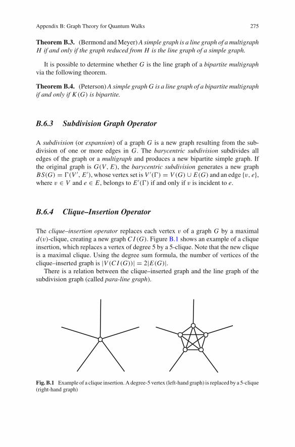
The clique–insertion operator replaces each vertex v of a graph G by a maximald(v)-clique, creating a new graph C I (G). Figure B.1 shows an example of a cliqueinsertion, which replaces a vertex of degree 5 by a 5-clique. Note that the new cliqueis a maximal clique. Using the degree sum formula, the number of vertices of theclique–inserted graph is |V (C I (G))| = 2|E(G)|.

There is a relation between the clique–inserted graph and the line graph of thesubdivision graph (called para-line graph).

Fig. B.1 Example of a clique insertion.A degree-5 vertex (left-hand graph) is replaced by a 5-clique(right-hand graph)


Theorem B.5. (Sampathkumar) The para-line graph of G is isomorphic to theclique–inserted graph C I (G).

B.7 Coloring

A coloring of a graph is a labeling of the vertices with colors so that no two verticessharing the same edge have the same color. The smallest number of colors needed tocolor a graph is called chromatic number, denoted by χ( ). A graph that can beassigned a coloring with k colors is k-colorable and is k-chromatic if its chromaticnumber is exactly k.

Theorem B.6. (Brooks) χ( ) ≤ �( ) for a graph , unless is a complete graphor an odd cycle.

The complete graph with N vertices has χ( ) = N and �( ) = N − 1. Oddcycles have χ( ) = 3 and�( ) = 2. For these graphs the bound χ( ) ≤ �( ) + 1is the best possible. In all other cases, the bound χ( ) ≤ �( ) is given by Brooks’theorem.

The concept of coloring can be applied to the edge set of a loop free graph. Anedge coloring is a coloring of the edges so that no vertex is incident to two edges ofthe same color. The smallest number of colors needed for an edge coloring is calledthe chromatic index or edge-chromatic number, denoted by χ ′( ).

Theorem B.7. (Vizing) A graph of maximal degree �( ) has edge-chromaticnumber �( ) or �( ) + 1, that is, �( ) ≤ χ ′( ) ≤ �( ) + 1.

Since at least �( ) colors are always necessary for edge coloring, the set ofall graphs may be partitioned into two classes: (1) class 1 graphs for which �( )

colors are sufficient and (2) class 2 graphs for which �( ) + 1 colors are necessary.Examples of graphs in class 1 are: complete graphs KN for even N , bipartite graphs.Examples of graph in class 2 are: regular graphs with an odd number of verticesN > 1 (includes complete graphs KN for odd N ≥ 3), Petersen graph. To determinewhether an arbitrary graph is in class 1 is NP-complete. There are asymptotic resultsin literature showing that the proportion of graphs in class 2 is very small.

Given a graph in class 2, we describe two ways to modify the graph in orderto create a new graph in class 1: (1) Add a leaf to each vertex of , or (2) make anidentical copy of and add edges connecting the pairs of identical vertices.

B.8 Diameter

The geodesic distance (simply distance) between two vertices in graph G(V, E) isthe number of edges in a shortest path connecting them. The eccentricity ε(v) of a


vertex v is the greatest geodesic distance between v and any other vertex, that is, it ishow far a vertex is from the vertex most distant from it in the graph. The diameter dof a graph is d = maxv∈V ε(v), that is, it is the maximum eccentricity of any vertexin the graph or the greatest distance between any pair of vertices.

B.9 Directed Graph

A directed graph or digraph G is defined by a vertex set V (G), an arc set A(G), anda function assigning each arc an ordered pair of vertices. We use the notation (v, v′)for an ordered pair of vertices, where v is the tail and v′ is the head, and (v, v′) iscalled directed edge or simply arc. A digraph is a simple digraph if each orderedpair is the head and tail of at most one arc. The underlying graph of a digraph G isthe graph obtained by considering the arcs of G as unordered pairs.

If (v, v′) and (v′, v) are in A(G), the set with (v, v′) and (v′, v) is called a pairof symmetric arcs. A symmetric directed graph G or symmetric digraph is a digraphwhose arc set comprises pairs of symmetric arcs, that is, if (v, v′) ∈ A(G), then(v′, v) ∈ A(G). Figure B.2 depicts an example of a symmetric digraph G and itsunderlying simple graph H .

The outdegree d+(v) is the number of arcs with tail v. The indegree d−(v) is thenumber of arcs with head v. The definitions of out-neighborhood, in-neighborhood,minimum and maximum indegree and outdegree are straightforward generalizationsof the corresponding undirected ones. A local sink or simply sink is a vertex withoutdegree zero, and a local source or simply source is a vertex with indegree zero.A global sink is a vertex which is reached by all other vertices. A global source A isa vertex which reaches all other vertices.

A directed cycle graph is a directed version of a cycle graph, where all edges areoriented in the same direction. A directed acyclic graph is a finite directed graph withno directed cycles. The moral graph of a directed acyclic graph G is a simple graphthat is obtained from the underlying simple graph of G by adding edges between allpairs of vertices that have a common child (in G).

Fig. B.2 Example of a symmetric digraph G and its underlying simple graph H


B.10 Some Named Graphs

B.10.1 Johnson Graphs

Let [N ] be the set {1, . . . , N }. There are(Nk

)k-subsets of [N ], where a k-subset

is a subset of [N ] with k elements. Let us define the Johnson graph J (N , k). Thevertices of J (N , k) are the k-subsets of [N ], and two vertices are adjacent if and onlyif their intersection has size (k − 1). If k = 1, J (N , 1) is the complete graph KN .J (N , k) and J (N , N − k) are the same graphs after renaming the vertices. J (N , k)is a regular graph with degree k (N − k). The diameter of J (N , k) is min(k, N − k).

B.10.2 Kneser Graphs

Let [N ] be the set {1, . . . , N }. A k-subset is a subset of [N ] with k elements. TheKneser graph KGN ,k is the graph whose vertices are the k-subsets, and two verticesare adjacent if and only if the two corresponding sets are disjoint. If k = 1, KGN ,1 isthe complete graph KN . KGN ,k is a regular graph with degree

(N−kk

). The diameter

of KGN ,k is �(k − 1)/(N − 2k)� + 1. The Petersen graph, depicted in Fig. B.3, isa Kneser graph KG5,2. It is in class 2 because it is 3-regular and its edge-chromaticnumber is 4.

B.10.3 Cayley Graphs

ACayley graph (G, S) encodes the structure of a groupG described by a generatingset S in the context of abstract algebra.

Definition B.8. A group is a nonempty set G together with a binary operation ·(called product), which satisfies the following requirements:

• (Closure) For all a, b in G, a · b is also in G.• (Associativity) For all a, b, c in G, (a · b) · c = a · (b · c).

Fig. B.3 Petersen graph


• (Identity) There exists an identity element e in G such that, for every element a inG, a · e = e · a = a.

• (Inverse) For eacha inG, there exists an element b inG, such thata · b = b · a = e,where e is the identity element. Element b is denoted by a−1.

The order of a group is its number of elements. A group is finite if its order isfinite. A group is commutative or abelian if the binary operation is commutative. Agenerating set of a group G is a subset S ⊂ G such that every element of G can beexpressed as the product of finitely many elements of S and their inverses. From nowon, we suppose that S is finite. S is called symmetric if S = S−1, that is, whenevers ∈ S, s−1 is also in S.

A subgroup of a group G is a subset H of G such that H is a group with the sameproduct operation of G. No proper subgroup of group G can contain a generating setof G.

The Cayley graph (G, S) is a directed graph defined as follows. The vertex setV ( ) is G, and the arc (a, b) is in A( ) if and only if b = a · s for some s ∈ S,where a, b ∈ G.

If S is symmetric and e �= S, the Cayley graph (G, S) is a |S|-regular simplegraph. It is a difficult problem to decide whether a Cayley graph of a group describedby a symmetric generating set is in class 1 or class 2. There is a remarkable conjecturestudied over decades:

Conjecture B.9. (Stong) All undirected Cayley graphs of groups of even order arein class 1.

Further Reading

Graph theory has many applications, and it is easy to get lost and waste time aftertaking some wrong direction. No danger comes from those introductory books [53,139, 314, 326]. Before starting to read an advanced book, check whether it is reallynecessary to go further. In the context of quantum walks, the survey [58] is use-ful. Harary’s book [138] is excellent (there is a new edition by CRC Press). Othersuggestions are [75, 102, 121]. Wikipedia (English version) is an excellent place toobtain quickly the definition or the main properties of a concept in graph theory, andhttp://www.graphclasses.org is a Web site used by researchers in graphtheory. Some results compiled in this Appendix are described in papers [259, 289,304, 318, 347].

Appendix CClassical Hitting Time

Consider a connected, nondirected, and non-bipartite graph Γ (X, E), where X ={x1, . . . , xn} is the vertex set and E is the edge set. The hitting time of a classicalrandom walk on this graph is the expected time for the walker to reach a markedvertex for the first time, once given the initial conditions. We may have more thanone marked vertex defined by a subset M ∈ X . In this case, the hitting time is theexpected time for the walker to reach a vertex in M for the first time.

If px x ′(t) is the probability of the walker to reach x ′ for the first time at time thaving left x at t = 0, the hitting time from vertex x to x ′ is

Hx x ′ =∞∑

t=0

t px x ′(t). (C.1)

Define Hx x = 0 when the departure and arrival vertices are the same.For example, the probability px x ′(t) at time t = 1 when x �= x ′ for the complete

graph with n vertices is 1/(n − 1), because the walker has n − 1 possible verticesto move in the first step. To arrive at vertex x ′ at time t = 2 for the first time, thewalker must visit one of n − 2 vertices different from x and x ′. The probabilityis (n − 2)/(n − 1). After this visit, it must go directly to vertex x ′, which occurswith probability 1/(n − 1). Therefore, px x ′(2) = (n − 2)/(n − 1)2. Generalizingthis argumentation, we obtain px x ′(t) = (n − 2)t−1/(n − 1)t . Then,

Hx x ′ =∞∑

t=0

t(n − 2)t−1

(n − 1)t.

Using the identity∑∞

t=0 tαt = α/(1 − α)2, which is valid for 0 < α < 1, we obtain

Hx x ′ = n − 1. (C.2)

Usually, the hitting time depends on x and x ′, but the complete graph is an exception.In the general case, Hx x ′ can be different from Hx ′x .


281

282 Appendix C: Classical Hitting Time

The notion of hitting time from a vertex to a subset can be formalized as follows:Suppose that M is a nonempty subset of X with cardinality m and define pxM(t) asthe probability that the walker reaches any of the vertices in M for the first time attime t having left x at t = 0. The hitting time from x to M is

HxM =∞∑

t=0

t pxM(t). (C.3)

Again, we define HxM = 0 if x ∈ M .Let us use an extended notion of hitting time when the walker starts from a

probability distribution. In the former case, the probability to depart from vertex xis 1 and the probability to depart from any other vertex is 0. Suppose that the walkerstarts with a distribution σ , that is, at the initial time the probability of the walker tobe at vertex x is σx . The most used initial distributions are the uniform distributionσx = 1/n and the stationary distribution, which is defined ahead. In any case, theinitial distribution must satisfy

∑x∈X σx = 1. The hitting time from σ to M is

HσM =∑

x∈Xσx HxM . (C.4)

That is, HσM is the expected value of the hitting time HxM from x to M weightedwith distribution σ .

Exercise C.1. Show that for the complete graph

HxM = n − 1

m

if x /∈ M .

Exercise C.2. Show that for the complete graph

HσM = (n − m)(n − 1)

mn

if σ is the uniform distribution. Why HσM ≈ HxM for n � m?

C.1 Hitting Time Using the Stationary Distribution

Equations (C.1) and (C.3) are troublesome for the practical calculation of the hittingtime of random walks on graphs. Fortunately, there are alternative methods. Thebest-known method uses a recursive method. Let us illustrate this method using thecomplete graph. We want to calculate Hx x ′ . The walker departs from x and movesdirectly to x ′ with probability 1/(n − 1) spending one time unit. With probability

Appendix C: Classical Hitting Time 283

(n − 2)/(n − 1), the walker moves to vertex x ′′ different from x ′ and therefore itspends one time unit plus the expected time to go from x ′′ to x ′, which is Hx x ′ . Wehave established the following recursive equation:

Hx x ′ = 1

n − 1+ n − 2

n − 1

(1 + Hx x ′

), (C.5)

the solution of which is equal to (C.2).This method works for an arbitrary graph. If Vx is the neighborhood of x , the

cardinality of Vx is the degree of x denoted by d(x). To help this calculation, weassume that the distance between x and x ′ is greater than 1. So, the walker will departfrom x and will move to the neighboring vertex x ′′ with probability 1/d(x) spendingone time unit. Now, we must add this result to the expected time to move from x ′′ tox ′. This has to be performed for all vertices x ′′ in the neighborhood of x . We obtain

Hx x ′ = 1

d(x)

∑

x ′′∈Vx

(1 + Hx ′′ x ′

). (C.6)

Equation (C.5) is a special case of (C.6), because for the complete graphd(x) = n − 1and Hx ′′ x ′ = Hx x ′ unless x ′′ = x ′. The case x ′′ = x ′ generates the first term in (C.5).The remaining n − 2 cases generate the second term. This shows that (C.6) is generaland the distance between x and x ′ need not be greater than 1. However, we cannottake x = x ′ (distance 0) since the left-hand side is zero and the right-hand side is not.

The goal now is to solve (C.6) in terms of the hitting time Hx x ′ . This task isfacilitated if (C.6) is converted to the matrix form. If H is a square n-dimensionalmatrix with entries Hx x ′ , the left-hand side will be converted into H and the right-hand side must be expanded. Using that

px x ′ ={ 1

d(x) , if x ′ is adjacent to x;0, otherwise,

(C.7)

we obtain the following matrix equation:

H = J + PH + D, (C.8)

where J is a matrix with all entries equal to 1, P is the right stochastic matrix, andD is a diagonal matrix that should be introduced to validate the matrix equation forthe diagonal elements. P is also called transition matrix or probability matrix, as wehave discussed in Chap. 3.

The diagonal matrix D can be calculated using the stationary distribution π ,which is the distribution that satisfies equation πT · P = πT . It is also called limitingor equilibrium distribution. For connected, nondirected, and non-bipartite graphsΓ (X, E), there is always a limiting distribution. By left multiplying (C.8) by πT , weobtain


Dx x = − 1

πx,

where πx is the x th entry of π .Equation (C.8) can be written as (I − P)H = J + D. When we try to find H

using this equation, we deal with the fact that (I − P) is a noninvertible matrix,because 1 is a 0-eigenvector of (I − P), where 1 is the vector with all entries equalto 1. This means that equation (I − P)X = J + D has more than one solution X .In fact, if matrix X is a solution, then X + 1 · vT is also a solution for any vector v.However, having at hand a solution X of this equation does not guarantee that wehave found H . There is a way to verify whether X is a correct solution by using thatHx x must be zero for all x . A solution of equation (I − P)X = J + D is

X = (I − P + 1 · πT)−1

(J + D), (C.9)

as can be checked by solving Exercise C.3. Now we add a term of type 1 · vT tocancel out the diagonal entries of X , and we obtain

H = X − 1 · vT , (C.10)

where the entries of vector v are the diagonal entries of X , that is, vx = Xx x .

Exercise C.3. LetM = I − P + 1 · πT .

1. Show that M is invertible.2. Using equations πT · P = πT , P · 1 = 1, and

M−1 =∞∑

t=0

(I − M)t ,

show that

M−1 = 1 · πT +∞∑

t=0

(Pt − 1 · πT

).

3. Show that solution (C.9) satisfies equation (I − P)X = J + D.4. Show that matrix H given by (C.10) satisfies Hx x = 0.

Exercise C.4. Find the stochastic matrix of the complete graph with n vertices.Using the fact that the stationary distribution is uniform in this graph, find matrix Xusing (C.9) and then find matrix H using (C.10). Check the results with (C.2).


C.2 Hitting Time Without the Stationary Distribution

There is an alternative method for calculating the hitting time that does not use thestationary distribution. We describe the method using HσM as defined in (C.4). Thevertices in M are called marked vertices. Consider the symmetric digraph whoseunderlying graph is Γ (X, E). Now we define a modified digraph, which is obtainedfrom the symmetric digraph by converting all arcs leaving the marked vertices intoloops, whilemaintaining unchanged the incoming ones. This means that if the walkerreaches a marked vertex, the walker will stay there forever. To calculate the hittingtime, the original undirected graph and the modified digraph are equivalent. How-ever, the stochastic matrices are different. Let us denote the stochastic matrix of themodified graph by P ′, whose entries are

p′xy =

{pxy, x /∈ M;δxy, x ∈ M.

(C.11)

What is the probability of finding the walker in X\M at time t before visiting M?Let σ (0) be the initial probability distribution on the vertices of the original graphviewed as a row vector. Then, the distribution after t steps is

σ (t) = σ (0) · Pt . (C.12)

Let 1 be the column n-vector with all entries equal to 1. Define 1X\M as the columnn-vector with n − m entries equal to 1 corresponding to the vertices that are in X\Mand m entries equal to zero corresponding to the vertices are in M . The probabilityof finding the walker in X\M at time t is σ (t) · 1X\M . However, this expression is notuseful for calculating the hitting time, because the walker has already visited M . Wewant to find the probability of the walker being in X\M at time t having not visitedM . This result is obtained if we use matrix P ′ instead of P in (C.12). In fact, if theevolution is driven by matrix P ′ and the walker has visited M , it remains imprisonedin M forever. Therefore, if the walker is found in X\M , it has certainly not visitedM . The probability of finding the walker in X\M at time t without having visitedM is σ (0) · (P ′)t · 1X\M .

In (C.3), we have calculated the average time to reach a marked vertex for thefirst time employing the usual formula for calculating weighted averages. When thevariable t assumes nonnegative integer values, there is an alternative formula forcalculating this average. This formula applies to this context because time t is thenumber of steps. Let T be the number of steps to reach a marked vertex for the firsttime, and let p(T ≥ t) be the probability of reaching M for the first time for anynumber of steps T equal to or greater than t . If the initial condition is distribution σ ,the hitting time can be equivalently defined by formula

Hσ M =∞∑

t=1

p(T ≥ t). (C.13)


To verify the equivalence of this new formula with the previous one, note that

p(T ≥ t) =∞∑

j=t

p(T = j), (C.14)

where p(T = t) is the probability of reaching M for the first time with exactly tsteps. Using (C.14) and (C.13), we obtain

Hσ M =∞∑

j=1

j∑

t=1

p(T = j)

=∞∑

j=1

j p(T = j). (C.15)

This last equation is equivalent to (C.3).We can give another interpretation for probability p(T ≥ t). If the walker reaches

M at T ≥ t , then in the first t − 1 steps it will still be in X\M , that is, it will be on oneof the unmarked vertices without having visited M . We have learned in a previousparagraph that the probability of the walker being in X\M at time t without havingvisited M is σ (0) · (P ′)t−1 · 1X\M . Then,

p(T ≥ t) = σ (0) · (P ′)t−1 · 1X\M . (C.16)

Define PM as a square (n − m)-matrix obtained from P by deleting the rows andcolumns corresponding to vertices ofM . DefineσM and1M using the sameprocedure.Analyzing the entries that do not vanish after multiplying the matrices on the right-hand side of (C.16), we conclude that

p(T ≥ t) = σ(0)M

· Pt−1M

· 1M . (C.17)

Using the above equation and (C.13), we obtain

Hσ M = σ(0)M

·( ∞∑

t=0

PtM

)· 1M

= σ(0)M

· (I − PM

)−1 · 1M . (C.18)

Matrix (I − PM) is always invertible for connected, nondirected, and non-bipartitegraphs. This result follows from the fact that 1 is not an eigenvector of PM , and hence(I − PM) has no eigenvalue equal to 0.

The strategy used to obtain (C.18) is used to define the quantum hitting time inSzegedy’s model.


Exercise C.5. Use (C.18) to find the hitting time of a random walk on the completegraph with n vertices, and compare the results with Exercises C.1 and C.2.

Further Reading

The classical hitting time is described inmany references, for instance, [11, 215, 235,245]. The last chapter of [235] describes in detail the Perron–Frobenius theorem,which is important in the context of this appendix.

References

1. Aaronson, S., Ambainis, A.: Quantum search of spatial regions. In: Theory of Computing,pp. 200–209 (2003)

2. Aaronson, S., Shi, Y.: Quantum lower bounds for the collision and the element distinctnessproblems. J. ACM 51(4), 595–605 (2004)

3. Abal, G., Donangelo, R., Forets, M., Portugal, R.: Spatial quantum search in a triangularnetwork. Math. Struct. Comput. Sci. 22(03), 521–531 (2012)

4. Abal, G., Donangelo, R., Marquezino, F.L., Portugal, R.: Spatial search on a honeycombnetwork. Math. Struct. Comput. Sci. 20(6), 999–1009 (2010)

5. Abreu, A., Cunha, L., Fernandes, T., de Figueiredo, C., Kowada, L., Marquezino, F., Posner,D., Portugal, R.: The graph tessellation cover number: extremal bounds, efficient algorithmsand hardness. In: Bender, M.A., Farach-Colton, M., Mosteiro, M.A. (eds.) LATIN 2018.Lecture Notes in Computer Science, vol. 10807, pp. 1–13. Springer, Berlin (2018)

6. Agliari, E., Blumen, A., Mülken, O.: Quantum-walk approach to searching on fractal struc-tures. Phys. Rev. A 82, 012305 (2010)

7. Aharonov, D.: Quantum computation - a review. In: Stauffer, D. (ed.) Annual Review ofComputational Physics, vol. VI, pp. 1–77. World Scientific, Singapore (1998)

8. Aharonov, D., Ambainis, A., Kempe, J., Vazirani, U.: Quantum walks on graphs. In: Proceed-ings of the 33th STOC, pp. 50–59. ACM, New York (2001)

9. Aharonov, Y., Davidovich, L., Zagury, N.: Quantum random walks. Phys. Rev. A 48(2),1687–1690 (1993)

10. Alberti,A.,Alt,W.,Werner, R.,Meschede,D.:Decoherencemodels for discrete-time quantumwalks and their application to neutral atom experiments. New J. Phys. 16(12), 123052 (2014)

11. Aldous, D., Fill, J.A.: Reversible Markov chains and random walks on graphs (2002). http://www.stat.berkeley.edu/~aldous/RWG/book.html

12. Alvir, R., Dever, S., Lovitz, B., Myer, J., Tamon, C., Xu, Y., Zhan, H.: Perfect state transferin laplacian quantum walk. J. Algebr. Comb. 43(4), 801–826 (2016)

13. Ambainis, A.: Quantumwalks and their algorithmic applications. Int. J. Quantum Inf. 01(04),507–518 (2003)

14. Ambainis, A.: Quantumwalk algorithm for element distinctness. In: Proceedings 45th AnnualIEEESymposium on Foundations of Computer Science FOCS, pp. 22–31.Washington (2004)

15. Ambainis, A.: Polynomial degree and lower bounds in quantum complexity: collision andelement distinctness with small range. Theory Comput. 1, 37–46 (2005)

16. Ambainis, A.: Quantum walk algorithm for element distinctness. SIAM J. Comput. 37(1),210–239 (2007)


289

http://www.stat.berkeley.edu/~aldous/RWG/book.html

http://www.stat.berkeley.edu/~aldous/RWG/book.html

290 References

17. Ambainis, A., Bach, E., Nayak, A., Vishwanath, A., Watrous, J.: One-dimensional quantumwalks. In: Proceedings of the 33th STOC, pp. 60–69. ACM, New York (2001)

18. Ambainis, A., Backurs, A., Nahimovs, N., Ozols, R., Rivosh, A.: Search by quantum walkson two-dimensional grid without amplitude amplification. In: Proceedings of the 7th TQC,Tokyo, Japan, pp. 87–97. Springer, Berlin (2013)

19. Ambainis, A., Kempe, J., Rivosh, A.: Coins make quantum walks faster. In: Proceedings ofthe 16th Annual ACM-SIAM Symposium on Discrete Algorithms SODA, pp. 1099–1108(2005)

20. Ambainis, A., Portugal, R., Nahimov, N.: Spatial search on grids with minimum memory.Quantum Inf. Comput. 15, 1233–1247 (2015)

21. Ampadu, C.: Return probability of the open quantum random walk with time-dependence.Commun. Theor. Phys. 59(5), 563 (2013)

22. Anderson, P.W.: Absence of diffusion in certain random lattices. Phys. Rev. 109, 1492–1505(1958)

23. Angeles-Canul, R.J., Norton, R.M., Opperman, M.C., Paribello, C.C., Russell, M.C., Tamon,C.: Quantum perfect state transfer on weighted join graphs. Int. J. Quantum Inf. 7(8), 1429–1445 (2009)

24. Apostol, T.M.: Calculus, Volume 1: One-Variable Calculus with an Introduction to LinearAlgebra. Wiley, New York (1967)

25. Arunachalam, S., De Wolf, R.: Optimizing the number of gates in quantum search. QuantumInf. Comput. 17(3–4), 251–261 (2017)

26. Asbóth, J.K.: Symmetries, topological phases, and bound states in the one-dimensional quan-tum walk. Phys. Rev. B 86, 195414 (2012)

27. Asbóth, J.K., Edge, J.M.: Edge-state-enhanced transport in a two-dimensional quantumwalk.Phys. Rev. A 91, 022324 (2015)

28. Axler, S.: Linear Algebra Done Right. Springer, New York (1997)29. Balu, R., Liu, C., Venegas-Andraca, S.E.: Probability distributions for Markov chain based

quantum walks. J. Phys. A: Math. Theor. 51(3), 035301 (2018)30. Barnett, S.: Quantum Information. Oxford University Press, New York (2009)31. Barr, K., Fleming, T., Kendon, V.: Simulation methods for quantum walks on graphs applied

to formal language recognition. Nat. Comput. 14(1), 145–156 (2015)32. Barr, K.E., Proctor, T.J., Allen, D., Kendon, V.M.: Periodicity and perfect state transfer in

quantum walks on variants of cycles. Quantum Inf. Comput. 14(5–6), 417–438 (2014)33. Bašic,M.: Characterization of quantum circulant networks having perfect state transfer. Quan-

tum Inf. Process. 12(1), 345–364 (2013)34. Beame, P., Saks, M., Sun, X., Vee, E.: Time-space trade-off lower bounds for randomized

computation of decision problems. J. ACM 50(2), 154–195 (2003)35. Bednarska, M., Grudka, A., Kurzynski, P., Luczak, T., Wójcik, A.: Quantum walks on cycles.

Phys. Lett. A 317(1–2), 21–25 (2003)36. Bednarska, M., Grudka, A., Kurzynski, P., Luczak, T., Wójcik, A.: Examples of non-uniform

limiting distributions for the quantumwalk on even cycles. Int. J. Quantum Inf. 2(4), 453–459(2004)

37. Belovs, A.: Learning-graph-based quantum algorithm for k-distinctness. In: IEEE 53rd An-nual Symposium on Foundations of Computer Science, pp. 207–216 (2012)

38. Belovs, A., Childs, A.M., Jeffery, S., Kothari, R., Magniez, F.: Time-efficient quantum walksfor 3-distinctness. In: Proceedings of the 40th International Colloquium ICALP, Riga, Latvia,2013, pp. 105–122. Springer, Berlin (2013)

39. Benedetti, C.,Buscemi, F.,Bordone, P., Paris,M.G.A.:Non-Markovian continuous-timequan-tum walks on lattices with dynamical noise. Phys. Rev. A 93, 042313 (2016)

40. Benenti, G., Casati, G., Strini, G.: Principles of Quantum Computation And Information:Basic Tools And Special Topics. World Scientific Publishing, River Edge (2007)

41. Benioff, P.: Space Searches with a Quantum Robot. AMS ContemporaryMathematics Series,vol. 305. American Mathematical Society, Providence (2002)

References 291

42. Bennett, C.H., Bernstein, E., Brassard, G., Vazirani, U.V.: Strengths and weaknesses of quan-tum computing. SIAM J. Comput. 26(5), 1510–1523 (1997)

43. Bergou, J.A., Hillery, M.: Introduction to the Theory of Quantum Information Processing.Springer, New York (2013)

44. Bernard, P.-A., Chan, A., Loranger, É., Tamon, C., Vinet, L.: A graph with fractional revival.Phys. Lett. A 382(5), 259–264 (2018)

45. Bernasconi, A., Godsil, C., Severini, S.: Quantum networks on cubelike graphs. Phys. Rev.A 78, 052320 (2008)

46. Berry, S.D., Bourke, P., Wang, J.B.: QwViz: visualisation of quantum walks on graphs. Com-put. Phys. Commun. 182(10), 2295–2302 (2011)

47. Bhattacharya, N., van Linden van den Heuvell, H.B., Spreeuw, R.J.C., : Implementation ofquantum search algorithm using classical Fourier optics. Phys. Rev. Lett. 88, 137901 (2002)

48. Bian, Z.-H., Li, J., Zhan, X., Twamley, J., Xue, P.: Experimental implementation of a quantumwalk on a circle with single photons. Phys. Rev. A 95, 052338 (2017)

49. Biham, O., Nielsen, M.A., Osborne, T.J.: Entanglement monotone derived from Grover’salgorithm. Phys. Rev. A 65, 062312 (2002)

50. Boada, O., Novo, L., Sciarrino, F., Omar, Y.: Quantum walks in synthetic gauge fields withthree-dimensional integrated photonics. Phys. Rev. A 95, 013830 (2017)

51. Boettcher, S., Falkner, S., Portugal, R.: Renormalization group for quantum walks. J. Phys.Conf. Ser. 473(1), 012018 (2013)

52. Boettcher, S., Li, S.: Analysis of coined quantum walks with renormalization. Phys. Rev. A97, 012309 (2018)

53. Bondy, A., Murty, U.S.R.: Graph Theory. Graduate Texts in Mathematics. Springer, London(2011)

54. Bose, S.: Quantum communication through an unmodulated spin chain. Phys. Rev. Lett. 91,207901 (2003)

55. Botsinis, P., Babar, Z., Alanis, D., Chandra, D., Nguyen, H., Ng, S.X., Hanzo, L.: Quantumerror correction protects quantum search algorithms against decoherence. Sci. Rep. 6, 38095(2016)

56. Bougroura, H., Aissaoui, H., Chancellor, N., Kendon, V.: Quantum-walk transport propertieson graphene structures. Phys. Rev. A 94, 062331 (2016)

57. Boyer,M., Brassard, G., Høyer, P., Tapp,A.: Tight bounds on quantum searching. ForstschritteDer Physik 4, 820–831 (1998)

58. Brandstädt, A., Le, V.B., Spinrad, J.P.: Graph Classes: A Survey. SIAM, Philadelphia (1999)59. Brassard, G., Høyer, P., Mosca, M., Tapp, A.: Quantum amplitude amplification and estima-

tion. Quantum Computation and Quantum Information Science. AMS Contemporary Math-ematics Series, vol. 305, pp. 53–74. American Mathematical Society, Providence (2002)

60. Brassard, G., Høyer, P., Tapp, A.: Quantum cryptanalysis of hash and claw-free functions.In: Proceedings of the 3rd Latin American Symposium LATIN’98, pp. 163–169. Springer,Berlin (1998)

61. Breuer, H.P., Petruccione, F.: The Theory of Open Quantum Systems. Oxford UniversityPress, Oxford (2002)

62. Bru, L.A., de Valcárcel, G.J., di Molfetta, G., Pérez, A., Roldán, E., Silva, F.: Quantum walkon a cylinder. Phys. Rev. A 94, 032328 (2016)

63. Bruderer, M., Plenio, M.B.: Decoherence-enhanced performance of quantum walks appliedto graph isomorphism testing. Phys. Rev. A 94, 062317 (2016)

64. Buhrman, H., Dürr, C., Heiligman, M., Høyer, P., Magniez, F., Santha, M., de Wolf, R.:Quantum algorithms for element distinctness. SIAM J. Comput. 34(6), 1324–1330 (2005)

65. Byrnes, T., Forster, G., Tessler, L.: Generalized Grover’s algorithm for multiple phase inver-sion states. Phys. Rev. Lett. 120, 060501 (2018)

66. Cáceres, M.O.: On the quantum CTRW approach. Eur. Phys. J. B 90(4), 74 (2017)67. Cameron, S., Fehrenbach, S., Granger, L., Hennigh, O., Shrestha, S., Tamon, C.: Universal

state transfer on graphs. Linear Algebra Appl. 455, 115–142 (2014)

292 References

68. Carteret, H.A., Ismail, M.E.H., Richmond, B.: Three routes to the exact asymptotics for theone-dimensional quantum walk. J. Phys. A: Math. Gen. 36(33), 8775–8795 (2003)

69. Carvalho, S.L., Guidi, L.F., Lardizabal, C.F.: Site recurrence of open and unitary quantumwalks on the line. Quantum Inf. Process. 16(1), 17 (2016)

70. Cedzich, C., Geib, T., Grünbaum, F.A., Stahl, C., Velázquez, L., Werner, A.H., Werner, R.F.:The topological classification of one-dimensional symmetric quantum walks. Ann. HenriPoincaré 19(2), 325–383 (2018)

71. Chakraborty, K., Maitra, S.: Application of Grover’s algorithm to check non-resiliency of aboolean function. Cryptogr. Commun. 8(3), 401–413 (2016)

72. Chakraborty, S., Novo, L., Di Giorgio, S., Omar, Y.: Optimal quantum spatial search onrandom temporal networks. Phys. Rev. Lett. 119, 220503 (2017)

73. Chan, A., Coutinho, G., Tamon, C., Vinet, L., Zhan, H.: Quantum fractional revival on graphs(2018). arXiv:1801.09654

74. Chandrashekar, C.M., Busch, T.: Quantum percolation and transition point of a directeddiscrete-time quantum walk. Sci. Rep. 4, 6583 (2014)

75. Chartrand, G., Lesniak, L., Zhang, P.: Graphs&Digraphs. Chapman&Hall/CRC, BocaRaton(2010)

76. Chiang, C.-F., Gomez, G.: Hitting time of quantum walks with perturbation. Quantum Inf.Process. 12(1), 217–228 (2013)

77. Chiang, C.-F., Nagaj, D., Wocjan, P.: Efficient circuits for quantum walks. Quantum Inf.Comput. 10(5–6), 420–434 (2010)

78. Childs, A.M.: Universal computation by quantum walk. Phys. Rev. Lett. 102, 180501 (2009)79. Childs, A.M.: On the relationship between continuous- and discrete-time quantum walk.

Commun. Math. Phys. 294(2), 581–603 (2010)80. Childs, A.M., Eisenberg, J.M.: Quantum algorithms for subset finding. Quantum Inf. Comput.

5(7), 593–604 (2005)81. Childs, A.M., Farhi, E., Gutmann, S.: An example of the difference between quantum and

classical random walks. Quantum Inf. Process. 1(1), 35–43 (2002)82. Childs, A.M., Goldstone, J.: Spatial search and the Dirac equation. Phys. Rev. A 70, 042312

(2004)83. Christandl, M., Datta, N., Ekert, A., Landahl, A.J.: Perfect state transfer in quantum spin

networks. Phys. Rev. Lett. 92, 187902 (2004)84. Cohen-Tannoudji, C., Diu, B., Laloe, F.: QuantumMechanics. Wiley-Interscience, New York

(2006)85. Connelly, E., Grammel, N., Kraut, M., Serazo, L., Tamon, C.: Universality in perfect state

transfer. Linear Algebra Appl. 531, 516–532 (2017)86. Coutinho, G.: Quantum walks and the size of the graph. Discret. Math. (2018).

arXiv:1802.0873487. Coutinho, G., Godsil, C.: Perfect state transfer in products and covers of graphs. Linear

Multilinear Algebra 64(2), 235–246 (2016)88. Coutinho, G., Godsil, C.: Perfect state transfer is poly-time. Quantum Inf. Comput. 17(5–6),

495–502 (2017)89. Coutinho,G., Portugal, R.: Discretization of continuous-time quantumwalks via the staggered

model with Hamiltonians. Nat. Comput. (2018). arXiv:1701.0342390. Cover, T.M., Thomas, J.: Elements of Information Theory. Wiley, New York (1991)91. Crespi, A., Osellame, R., Ramponi, R., Giovannetti, V., Fazio, R., Sansoni, L., De Nicola,

F., Sciarrino, F., Mataloni, P.: Anderson localization of entangled photons in an integratedquantum walk. Nat. Photonics 7(4), 322–328 (2013)

92. D’Ariano, G.M., Erba, M., Perinotti, P., Tosini, A.: Virtually abelian quantum walks. J. Phys.A: Math. Theor. 50(3), 035301 (2017)

93. de Abreu, A.S.: Tesselações em grafos e suas aplicações em computação quântica. Master’sthesis, UFRJ (2017)

94. de Abreu, A.S., Ferreira, M.M., Kowada, L.A.B., Marquezino, F.L.: QEDS: A classical sim-ulator for quantum element distinctness. Revista de Informática Teórica e Aplicada 23(2),51–66 (2016)

http://arxiv.org/abs/1801.09654



References 293

95. Derevyanko, S.: Anderson localization of a one-dimensional quantum walker. Sci. Rep. 8(1),1795 (2018)

96. d’Espagnat, B.: Conceptual Foundations of Quantum Mechanics. Westview Press, Boulder(1999)

97. Desurvire, E.: Classical and Quantum Information Theory: An Introduction for the TelecomScientist. Cambridge University Press, Cambridge (2009)

98. Dheeraj, M.N., Brun, T.A.: Continuous limit of discrete quantum walks. Phys. Rev. A 91,062304 (2015)

99. diMolfetta, G., Debbasch, F.: Discrete-time quantumwalks: continuous limit and symmetries.J. Math. Phys. 53(12), 123302 (2012)

100. Diao, Z., Zubairy, M.S., Chen, G.: A quantum circuit design for Grover’s algorithm. Z. Natur-forsch. A 57(8), 701–708 (2002)

101. Díaz, N., Donangelo, R., Portugal, R., Romanelli, A.: Transient temperature andmixing timesof quantum walks on cycles. Phys. Rev. A 94, 012305 (2016)

102. Diestel, R.: Graph Theory. Graduate Texts in Mathematics, vol. 173. Springer, New York(2012)

103. Dodd, J.L., Ralph, T.C., Milburn, G.J.: Experimental requirements for Grover’s algorithm inoptical quantum computation. Phys. Rev. A 68, 042328 (2003)

104. Domino, K., Glos, A., Ostaszewski, M.: Superdiffusive quantum stochastic walk definable onarbitrary directed graph. Quantum Info. Comput. 17(11–12), 973–986 (2017)

105. Du, Y.-M., Lu, L.-H., Li, Y.-Q.: A rout to protect quantum gates constructed via quantumwalks from noises. Sci. Rep. 8(1), 7117 (2018)

106. Dukes, P.R.: Quantum state revivals in quantum walks on cycles. Results Phys. 4, 189–197(2014)

107. Dunjko, V., Briegel, H.J.: Quantum mixing of Markov chains for special distributions. NewJ. Phys. 17(7), 073004 (2015)

108. Ellinas, D., Konstandakis, C.: Parametric quantum search algorithm as quantum walk: aquantum simulation. Rep. Math. Phys. 77(1), 105–128 (2016)

109. Endo, T., Konno, N., Obuse, H., Segawa, E.: Sensitivity of quantum walks to a boundary oftwo-dimensional lattices: approaches based on the CGMVmethod and topological phases. J.Phys. A: Math. Theor. 50(45), 455302 (2017)

110. Ermakov, V.L., Fung, B.M.: Experimental realization of a continuous version of the Groveralgorithm. Phys. Rev. A 66, 042310 (2002)

111. Falk, M.: Quantum search on the spatial grid (2013). arXiv:1303.4127112. Falloon, P.E., Rodriguez, J., Wang, J.B.: QSWalk: a mathematica package for quantum

stochastic walks on arbitrary graphs. Comput. Phys. Commun. 217, 162–170 (2017)113. Farhi, E., Gutmann, S.: Quantum computation and decision trees. Phys. Rev. A 58, 915–928

(1998)114. Feller, W.: An Introduction to Probability Theory and Its Applications. Wiley, New York

(1968)115. Foulger, I., Gnutzmann, S., Tanner, G.: Quantum walks and quantum search on graphene

lattices. Phys. Rev. A 91, 062323 (2015)116. Fujiwara, S., Hasegawa, S.: General method for realizing the conditional phase-shift gate and

a simulation of Grover’s algorithm in an ion-trap system. Phys. Rev. A 71, 012337 (2005)117. Galiceanu, M., Strunz, W.T.: Continuous-time quantum walks on multilayer dendrimer net-

works. Phys. Rev. E 94, 022307 (2016)118. Mc Gettrick, M., Miszczak, J.A.: Quantum walks with memory on cycles. Phys. A 399,

163–170 (2014)119. Ghosh, J.: Simulating Anderson localization via a quantum walk on a one-dimensional lattice

of superconducting qubits. Phys. Rev. A 89, 022309 (2014)120. Glos, A., Miszczak, J.A., Ostaszewski, M.: QSWalk.jl: Julia package for quantum stochastic

walks analysis (2018). arXiv:1801.01294121. Godsil, C., Royle, G.F.: Algebraic Graph Theory. Graduate Texts in Mathematics, vol. 207.

Springer, New York (2001)



294 References

122. Gönülol, M., Aydner, E., Shikano, Y., Müstecaplolu, Ö.E.: Survival probability in a quantumwalk on a one-dimensional lattice with partially absorbing traps. J. Comput. Theor. Nanosci.10(7), 1596–1600 (2013)

123. Gould, H.W.: Combinatorial Identities. Morgantown Printing and Binding Co., Morgantown(1972)

124. Goyal, S.K., Konrad, T., Diósi, L.: Unitary equivalence of quantum walks. Phys. Lett. A379(3), 100–104 (2015)

125. Graham,R.L.,Knuth,D.E., Patashnik,O.:ConcreteMathematics:AFoundation forComputerScience. Addison-Wesley, Reading (1994)

126. Griffiths, D.: Introduction to Quantum Mechanics. Benjamin Cummings, Menlo Park (2005)127. Grigoriev, D.: Karpinski, M., auf der Heide, F.M., Smolensky, R.: A lower bound for random-

ized algebraic decision trees. Comput. Complex. 6(4), 357–375 (1996)128. Grover, L.K.: A fast quantum mechanical algorithm for database search. In: Proceedings of

the 28th Annual ACM Symposium on Theory of Computing, STOC ’96, pp. 212–219. NewYork (1996)

129. Grover, L.K.: Quantum computers can search arbitrarily large databases by a single query.Phys. Rev. Lett. 79(23), 4709–4712 (1997)

130. Grover, L.K.: Quantum mechanics helps in searching for a needle in a haystack. Phys. Rev.Lett. 79(2), 325–328 (1997)

131. Grover, L.K.: Quantum computers can search rapidly by using almost any transformation.Phys. Rev. Lett. 80(19), 4329–4332 (1998)

132. Grover, L.K.: Trade-offs in the quantum search algorithm. Phys. Rev. A 66, 052314 (2002)133. Gudder, S.: Quantum Probability. Academic Press, San Diego (1988)134. LoGullo,N.,Ambarish, C.V., Busch, T.,Dell’Anna, L., Chandrashekar, C.M.,Chandrashekar,

C.M.: Dynamics and energy spectra of aperiodic discrete-time quantum walks. Phys. Rev. E96, 012111 (2017)

135. Hamada, M., Konno, N., Segawa, E.: Relation between coined quantum walks and quantumcellular automata. RIMS Kokyuroku 1422, 1–11 (2005)

136. Hamilton, C.S., Barkhofen, S., Sansoni, L., Jex, I., Silberhorn, C.: Driven discrete time quan-tum walks. New J. Phys. 18(7), 073008 (2016)

137. Hao, L., Li, J., Long, G.: Eavesdropping in a quantum secret sharing protocol based on Groveralgorithm and its solution. Sci. China Phys. Mech. Astron. 53(3), 491–495 (2010)

138. Harary, F.: Graph Theory. Addison-Wesley, Boston (1969)139. Hartsfield, N., Ringel, G.: Pearls in Graph Theory: A Comprehensive Introduction. Dover

Books on Mathematics. Dover Publications, New York (1994)140. Hayashi, M., Ishizaka, S., Kawachi, A., Kimura, G., Ogawa, T.: Introduction to Quantum

Information Science. Springer, Berlin (2014)141. He, Z., Huang, Z., Li, L., Situ, H.: Coherence of one-dimensional quantum walk on cycles.

Quantum Inf. Process. 16(11), 271 (2017)142. He, Z., Huang, Z., Li, L., Situ, H.: Coherence evolution in two-dimensional quantum walk on

lattice. Int. J. Quantum Inf. 16(02), 1850011 (2018)143. He, Z., Huang, Z., Situ, H.: Dynamics of quantum coherence in two-dimensional quantum

walk on finite lattices. Eur. Phys. J. Plus 132(7), 299 (2017)144. Hein, B., Tanner, G.: Quantum search algorithms on a regular lattice. Phys. Rev. A 82(1),

012326 (2010)145. Higuchi, Y., Konno, N., Sato, I., Segawa, E.: Spectral and asymptotic properties of Grover

walks on crystal lattices. J. Funct. Anal. 267(11), 4197–4235 (2014)146. Hirvensalo, M.: Quantum Computing. Springer, Berlin (2010)147. Ho, C.-L., Ide, Y., Konno, N., Segawa, E., Takumi, K.: A spectral analysis of discrete-time

quantum walks related to the birth and death chains. J. Stat. Phys. 171(2), 207–219 (2018)148. Hoffman, K.M., Kunze, R.: Linear Algebra. Prentice Hall, New York (1971)149. Holweck, F., Jaffali, H., Nounouh, I.: Grover’s algorithm and the secant varieties. Quantum

Inf. Process. 15(11), 4391–4413 (2016)150. Horn, R., Johnson, C.R.: Matrix Analysis. Cambridge University Press, Cambridge (1985)

References 295

151. Høyer, P.: Arbitrary phases in quantum amplitude amplification. Phys. Rev. A 62, 052304(2000)

152. Høyer, P., Komeili, M.: Efficient quantum walk on the grid with multiple marked elements.In: Vollmer, H., Vallée, B. (eds.) Proceedings of the 34th Symposium on Theoretical Aspectsof Computer Science STACS, vol. 66, pp. 42:1–14. Dagstuhl, Germany (2017)

153. Hsu, L.-Y.: Quantum secret-sharing protocol based on Grover’s algorithm. Phys. Rev. A 68,022306 (2003)

154. Hughes, B.D.: RandomWalks and Random Environments: Voloum 1 RandomWalks. OxfordUniversity Press, Oxford (1995)

155. Hughes, B.D.: RandomWalks and Random Environments: Volume 2 Random Environments.Oxford University Press, Oxford (1996)

156. Hush, M.R., Bentley, C.D.B., Ahlefeldt, R.L., James, M.R., Sellars, M.J., Ugrinovskii, V.:Quantum state transfer through time reversal of an optical channel. Phys. Rev. A 94, 062302(2016)

157. Ide, Y., Konno, N., Segawa, E.: Time averaged distribution of a discrete-time quantum walkon the path. Quantum Inf. Process. 11(5), 1207–1218 (2012)

158. Innocenti, L., Majury, H., Giordani, T., Spagnolo, N., Sciarrino, F., Paternostro, M., Ferraro,A.: Quantum state engineering using one-dimensional discrete-time quantum walks. Phys.Rev. A 96, 062326 (2017)

159. Itakura, Y.K.: Quantum algorithm for commutativity testing of a matrix set. Master’s thesis,University of Waterloo, Waterloo (2005)

160. Iwai, T., Hayashi, N., Mizobe, K.: The geometry of entanglement and Grover’s algorithm. J.Phys. A: Math. Theor. 41(10), 105202 (2008)

161. Izaac, J.A., Wang, J.B.: PyCTQW: a continuous-time quantum walk simulator on distributedmemory computers. Comput. Phys. Commun. 186, 81–92 (2015)

162. Izaac, J.A., Wang, J.B.: Systematic dimensionality reduction for continuous-time quantumwalks of interacting fermions. Phys. Rev. E 96, 032136 (2017)

163. Izaac, J.A., Zhan, X., Bian, Z., Wang, K., Li, J., Wang, J.B., Xue, P.: Centrality measure basedon continuous-time quantum walks and experimental realization. Phys. Rev. A 95, 032318(2017)

164. Jeffery, S.,Magniez, F., deWolf, R.:Optimal parallel quantumquery algorithms.Algorithmica79(2), 509–529 (2017)

165. Jin, W., Chen, X.: A desired state can not be found with certainty for Grover’s algorithm in apossible three-dimensional complex subspace. Quantum Inf. Process. 10(3), 419–429 (2011)

166. Johnston, N., Kirkland, S., Plosker, S., Storey, R., Zhang, X.: Perfect quantum state transferusing Hadamard diagonalizable graphs. Linear Algebra Appl. 531, 375–398 (2017)

167. Jones, J.A., Mosca, M., Hansen, R.H.: Implementation of a quantum search algorithm on aquantum computer. Nature 393(6683), 344–346 (1998)

168. Kaplan, M.: Quantum attacks against iterated block ciphers. Mat. Vopr. Kriptogr. 7, 71–90(2016)

169. Kargin, V.: Bounds for mixing time of quantum walks on finite graphs. J. Phys. A: Math.Theor. 43(33), 335302 (2010)

170. Kaye, P., Laflamme, R., Mosca, M.: An Introduction to Quantum Computing. Oxford Uni-versity Press, New York (2007)

171. Kedon, V.M., Tamon, C.: Perfect state transfer in quantumwalks on graphs. J. Comput. Theor.Nanosci. 8(3), 422–433 (2011)

172. Kempe, J.: Quantum random walks - an introductory overview. Contemp. Phys. 44(4), 302–327 (2003)

173. Kempe, J.: Discrete quantum walks hit exponentially faster. Probab. Theory Relat. Fields133(2), 215–235 (2005). arXiv:quant-ph/0205083

174. Kempton, M., Lippner, G., Yau, S.-T.: Perfect state transfer on graphs with a potential. Quan-tum Inf. Comput. 17(3–4), 303–327 (2017)

175. Kendon, V.: Decoherence in quantum walks - a review. Math. Struct. Comput. Sci. 17(6),1169–1220 (2007)

http://arxiv.org/abs/quant-ph/0205083

296 References

176. Kendon, V., Sanders, B.C.: Complementarity and quantum walks. Phys. Rev. A 71, 022307(2005)

177. Kirkland, S., Severini, S.: Spin-system dynamics and fault detection in threshold networks.Phys. Rev. A 83, 012310 (2011)

178. Kitaev, A.Y., Shen, A.H., Vyalyi, M.N.: Classical and Quantum Computation. AmericanMathematical Society, Boston (2002)

179. Koch, D., Hillery, M.: Finding paths in tree graphs with a quantum walk. Phys. Rev. A 97,012308 (2018)

180. Kollár, B., Novotný, J., Kiss, T., Jex, I.: Percolation induced effects in two-dimensional coinedquantum walks: analytic asymptotic solutions. New J. Phys. 16(2), 023002 (2014)

181. Komatsu, T., Konno, N.: Stationary amplitudes of quantum walks on the higher-dimensionalinteger lattice. Quantum Inf. Process. 16(12), 291 (2017)

182. Konno, N.: Quantum random walks in one dimension. Quantum Inf. Process. 1(5), 345–354(2002)

183. Konno, N.: Quantum walks. In: Franz, U., Schürmann, M. (eds.) Quantum Potential Theory.Lecture Notes in Mathematics, vol. 1954, pp. 309–452. Springer, Berlin (2008)

184. Konno, N., Ide, Y., Sato, I.: The spectral analysis of the unitary matrix of a 2-tessellablestaggered quantum walk on a graph. Linear Algebra Appl. 545, 207–225 (2018)

185. Konno, N., Mitsuhashi, H., Sato, I.: The discrete-time quaternionic quantum walk on a graph.Quantum Inf. Process. 15(2), 651–673 (2016)

186. Konno, N., Obata, N., Segawa, E.: Localization of the Grover walks on spidernets and freeMeixner laws. Commun. Math. Phys. 322(3), 667–695 (2013)

187. Konno, N., Portugal, R., Sato, I., Segawa, E.: Partition-based discrete-time quantum walks.Quantum Inf. Process. 17(4), 100 (2018)

188. Konno, N., Sato, I.: On the relation between quantum walks and zeta functions. Quantum Inf.Process. 11(2), 341–349 (2012)

189. Konno, N., Sato, I., Segawa, E.: The spectra of the unitary matrix of a 2-tessellable staggeredquantum walk on a graph. Yokohama Math. J. 62, 52–87 (2017)

190. Košík, J.: Two models of quantum random walk. Central Eur. J. Phys. 4, 556–573 (2003)191. Košík, J., Bužek, V., Hillery, M.: Quantum walks with random phase shifts. Phys. Rev. A 74,

022310 (2006)192. Krawec, W.O.: History dependent quantum walk on the cycle with an unbalanced coin. Phys.

A 428, 319–331 (2015)193. Krovi, H., Brun, T.A.: Quantum walks with infinite hitting times. Phys. Rev. A 74, 042334

(2006)194. Krovi, H., Brun, T.A.: Quantum walks on quotient graphs. Phys. Rev. A 75, 062332 (2007)195. Krovi, H., Magniez, F., Ozols, M., Roland, J.: Finding is as easy as detecting for quantum

walks. Automata, Languages and Programming. Lecture Notes in Computer Science, vol.6198, pp. 540–551. Springer, Berlin (2010)

196. Kutin, S.: Quantum lower bound for the collision problem with small range. Theory Comput.1, 29–36 (2005)

197. Laarhoven, T., Mosca, M., van de Pol, J.: Finding shortest lattice vectors faster using quantumsearch. Des. Codes Cryptogr. 77(2), 375–400 (2015)

198. Lam, H.T., Szeto, K.Y.: Ramsauer effect in a one-dimensional quantum walk with multipledefects. Phys. Rev. A 92, 012323 (2015)

199. Lang, S.: Linear Algebra. Undergraduate Texts in Mathematics and Technology. Springer,New York (1987)

200. Lang, S.: Introduction to Linear Algebra. Undergraduate Texts inMathematics. Springer, NewYork (1997)

201. Lara, P.C.S., Leão, A., Portugal, R.: Simulation of quantum walks using HPC. J. Comput. Int.Sci. 6, 21 (2015)

202. Lehman, L.: Environment-induced mixing processes in quantum walks. Int. J. Quantum Inf.12(04), 1450021 (2014)

References 297

203. Leuenberger, M.N., Loss, D.: Grover algorithm for large nuclear spins in semiconductors.Phys. Rev. B 68, 165317 (2003)

204. Li, D., Mc Gettrick, M., Gao, F., Xu, J., Wen, Q.-Y., Wen, Q.-Y.: Generic quantum walks withmemory on regular graphs. Phys. Rev. A 93, 042323 (2016)

205. Li, D., Mc Gettrick, M., Zhang, W.-W., Zhang, K.-J., Zhang, K.-J.: Quantum walks on twokinds of two-dimensional models. Int. J. Theor. Phys. 54(8), 2771–2783 (2015)

206. Li, P., Li, S.: Phase matching in Grover’s algorithm. Phys. Lett. A 366(1), 42–46 (2007)207. Li, P., Li, S.: Two improvements in Grover’s algorithm. Chin. J. Electron. 17(1), 100–104

(2008)208. Lin, J.-Y., Zhu, X., Wu, S.: Limitations of discrete-time quantum walk on a one-dimensional

infinite chain. Phys. Lett. A 382(13), 899–903 (2018)209. Lipton, R.J., Regan, K.W.: Quantum Algorithms via Linear Algebra: A Primer. MIT Press,

Boston (2014)210. Liu,C., Balu,R.: Steady states of continuous-time open quantumwalks.Quantum Inf. Process.

16(7), 173 (2017)211. Loke, T., Tang, J.W., Rodriguez, J., Small, M., Wang, J.B.: Comparing classical and quantum

pageranks. Quantum Inf. Process. 16(1), 25 (2016)212. Loke, T., Wang, J.B.: Efficient quantum circuits for continuous-time quantum walks on com-

posite graphs. J. Phys. A: Math. Theor. 50(5), 055303 (2017)213. Loke, T., Wang, J.B.: Efficient quantum circuits for Szegedy quantum walks. Ann. Phys. 382,

64–84 (2017)214. Long, G.L.: Grover algorithm with zero theoretical failure rate. Phys. Rev. A 64, 022307

(2001)215. Lovász, L.: Random walks on graphs: a survey. Comb. Paul Erdös Eighty 2, 1–46 (1993)216. Lovett, N.B., Cooper, S., Everitt,M., Trevers,M.,Kendon,V.:Universal quantumcomputation

using the discrete-time quantum walk. Phys. Rev. A 81, 042330 (2010)217. Lovett, N.B., Everitt, M., Heath, R.M., Kendon, V.: The quantum walk search algorithm:

factors affecting efficiency. Math. Struct. Comput. Sci. 67, 1–141 (2018)218. Lu, X., Yuan, J., Zhang, W.: Workflow of the Grover algorithm simulation incorporating

CUDA and GPGPU. Comput. Phys. Commun. 184(9), 2035–2041 (2013)219. Ma, B.-W., Bao, W.-S., Li, T., Li, F.-G., Zhang, S., Fu, X.-Q.: A four-phase improvement of

Grover’s algorithm. Chin. Phys. Lett. 34(7), 070305 (2017)220. Machida, T., Chandrashekar, C.M.: Localization and limit laws of a three-state alternate

quantum walk on a two-dimensional lattice. Phys. Rev. A 92, 062307 (2015)221. Machida, T., Chandrashekar, C.M., Konno, N., Busch, T.: Limit distributions for different

formsof four-state quantumwalks on a two-dimensional lattice.Quantum Inf.Comput.15(13–14), 1248–1258 (2015)

222. Mackay, T.D., Bartlett, S.D., Stephenson, L.T., Sanders, B.C.: Quantum walks in higherdimensions. J. Phys. A: Math. Gen. 35(12), 2745 (2002)

223. Magniez, F., Nayak, A.: Quantum complexity of testing group commutativity. Algorithmica48(3), 221–232 (2007)

224. Magniez, F., Nayak,A., Richter, P., Santha,M.:On the hitting times of quantumversus randomwalks. In: Proceedings of the 20th ACM-SIAM Symposium on Discrete Algorithms (2009)

225. Magniez, F., Nayak, A., Roland, J., Santha, M.: Search via quantum walk. In: Proceedings ofthe 39th ACM Symposium on Theory of Computing, pp. 575–584 (2007)

226. Magniez, F., Santha, M., Szegedy, M.: Quantum algorithms for the triangle problem. SIAMJ. Comput. 37(2), 413–424 (2007)

227. Makmal, A., Tiersch,M., Ganahl, C., Briegel, H.J.: Quantumwalks on embedded hypercubes:nonsymmetric and nonlocal cases. Phys. Rev. A 93, 022322 (2016)

228. Makmal, A., Zhu, M., Manzano, D., Tiersch, M., Briegel, H.J.: Quantum walks on embeddedhypercubes. Phys. Rev. A 90, 022314 (2014)

229. Manouchehri, K., Wang, J.: Physical Implementation of QuantumWalks. Springer, NewYork(2014)

298 References

230. Marinescu, D.C., Marinescu, G.M.: Approaching Quantum Computing. Pearson/PrenticeHall, Michigan (2005)

231. Marquezino, F.L., Portugal, R.: The qwalk simulator of quantum walks. Comput. Phys. Com-mun. 179(5), 359–369 (2008)

232. Marquezino, F.L., Portugal, R., Abal, G.: Mixing times in quantumwalks on two-dimensionalgrids. Phys. Rev. A 82(4), 042341 (2010)

233. Marquezino, F.L., Portugal, R., Abal, G., Donangelo, R.: Mixing times in quantum walks onthe hypercube. Phys. Rev. A 77, 042312 (2008)

234. Mermin, N.D.: Quantum Computer Science: An Introduction. Cambridge University Press,New York (2007)

235. Meyer, C.D.: Matrix Analysis and Applied Linear Algebra. SIAM, Philadelphia (2001)236. Meyer, D.A.: From quantum cellular automata to quantum lattice gases. J. Stat. Phys. 85(5),

551–574 (1996)237. Meyer, D.A.: Sophisticated quantum search without entanglement. Phys. Rev. Lett. 85, 2014–

2017 (2000)238. Meyer, D.A., Wong, T.G.: Connectivity is a poor indicator of fast quantum search. Phys. Rev.

Lett. 114, 110503 (2015)239. Mlodinow,L., Brun, T.A.:Discrete spacetime, quantumwalks, and relativisticwave equations.

Phys. Rev. A 97, 042131 (2018)240. Moore, C., Mertens, S.: The Nature of Computation. Oxford University Press, New York

(2011)241. Moore, C., Russell, A.: Quantum walks on the hypercube. In: Proceedings of the 6th Interna-

tionalWorkshop on Randomization andApproximation Techniques RANDOM, pp. 164–178.Springer, Berlin (2002)

242. Moqadam, J.K., Portugal, R., de Oliveira, M.C.: Quantum walks on a circle with optome-chanical systems. Quantum Inf. Process. 14(10), 3595–3611 (2015)

243. Khatibi Moqadam, J., de Oliveira, M.C., Portugal, R., Portugal, R.: Staggered quantum walkswith superconducting microwave resonators. Phys. Rev. B 95, 144506 (2017)

244. Mosca, M.: Counting by quantum eigenvalue estimation. Theor. Comput. Sci. 264(1), 139–153 (2001)

245. Motwani, R., Raghavan, P.: Randomized algorithms.ACMComput. Surv. 28(1), 33–37 (1996)246. Mülken, O., Blumen, A.: Continuous-time quantum walks: models for coherent transport on

complex networks. Phys. Rep. 502(2), 37–87 (2011)247. Nayak, A., Vishwanath, A.: Quantum walk on a line. DIMACS Technical Report 2000-43

(2000). arXiv:quant-ph/0010117248. Nielsen, M.A., Chuang, I.L.: Quantum Computation and Quantum Information. Cambridge

University Press, New York (2000)249. Novo, L., Chakraborty, S., Mohseni, M., Neven, H., Omar, Y.: Systematic dimensionality

reduction for quantum walks: optimal spatial search and transport on non-regular graphs. Sci.Rep. 5, 13304 (2015)

250. Ohno, H.: Unitary equivalent classes of one-dimensional quantum walks. Quantum Inf. Pro-cess. 15(9), 3599–3617 (2016)

251. Oliveira, A.C., Portugal, R., Donangelo, R.: Decoherence in two-dimensional quantumwalks.Phys. Rev. A 74, 012312 (2006)

252. Omnès, R.: UnderstandingQuantumMechanics. PrincetonUniversity Press, Princeton (1999)253. Pal, H., Bhattacharjya, B.: Perfect state transfer on gcd-graphs. Linear Multilinear Algebra

65(11), 2245–2256 (2017)254. Paparo,G.D.,Müller,M., Comellas, F.,Martin-Delgado,M.A.:QuantumGoogle in a complex

network. Sci. Rep. 3, 2773 (2013)255. Parthasarathy, K.R.: The passage from random walk to diffusion in quantum probability. J.

Appl. Probab. 25, 151–166 (1988)256. Patel, A., Raghunathan, K.S., Rungta, P.: Quantum random walks do not need a coin toss.

Phys. Rev. A 71, 032347 (2005)257. Peres, A.: Quantum Theory: Concepts and Methods. Springer, Berlin (1995)


References 299

258. Pérez, A., Romanelli, A.: Spatially dependent decoherence and anomalous diffussion of quan-tum walks. J. Comput. Theor. Nanosci. 10(7), 1591–1595 (2013)

259. Peterson, D.: Gridline graphs: a review in two dimensions and an extension to higher dimen-sions. Discret. Appl. Math. 126(2), 223–239 (2003)

260. Philipp, P., Portugal, R.: Exact simulation of coined quantum walks with the continuous-timemodel. Quantum Inf. Process. 16(1), 14 (2017)

261. Philipp, P., Tarrataca, L., Boettcher, S.: Continuous-time quantum search on balanced trees.Phys. Rev. A 93, 032305 (2016)

262. Piccinini, E., Benedetti, C., Siloi, I., Paris, M.G.A., Bordone, P.: GPU-accelerated algorithmsfor many-particle continuous-time quantum walks. Comput. Phys. Commun. 215, 235–245(2017)

263. Portugal, R.: Establishing the equivalence between Szegedy’s and coined quantum walksusing the staggered model. Quantum Inf. Process. 15(4), 1387–1409 (2016)

264. Portugal, R.: Staggered quantum walks on graphs. Phys. Rev. A 93, 062335 (2016)265. Portugal, R.: Element distinctness revisited. Quantum Inf. Process. 17(7), 163 (2018)266. Portugal, R., Boettcher, S., Falkner, S.: One-dimensional coinless quantum walks. Phys. Rev.

A 91, 052319 (2015)267. Portugal, R., deOliveira,M.C.,Moqadam, J.K.: Staggered quantumwalkswithHamiltonians.

Phys. Rev. A 95, 012328 (2017)268. Portugal, R., Fernandes, T.D.: Quantum search on the two-dimensional lattice using the stag-

gered model with Hamiltonians. Phys. Rev. A 95, 042341 (2017)269. Portugal, R., Santos, R.A.M., Fernandes, T.D., Gonçalves, D.N.: The staggered quantumwalk

model. Quantum Inf. Process. 15(1), 85–101 (2016)270. Portugal, R., Segawa, E.: Connecting coined quantum walks with Szegedy’s model. Interdis-

cip. Inf. Sci. 23(1), 119–125 (2017)271. Preiss, P.M., Ma, R., Tai, M.E., Lukin, A., Rispoli, M., Zupancic, P., Lahini, Y., Islam, R.,

Greiner, M.: Strongly correlated quantum walks in optical lattices. Science 347(6227), 1229–1233 (2015)

272. Preskill, J.: Lecture Notes on Quantum Computation (1998). http://www.theory.caltech.edu/~preskill/ph229

273. Reitzner, D., Hillery, M., Koch, D.: Finding paths with quantum walks or quantum walkingthrough a maze. Phys. Rev. A 96, 032323 (2017)

274. Reitzner, D., Nagaj, D., Buzek, V.: Quantum walks. Acta Phys. Slov. 61(6), 603–725 (2011)275. Ren, P., Aleksic, T., Emms, D., Wilson, R.C., Hancock, E.R.: Quantum walks, Ihara zeta

functions and cospectrality in regular graphs. Quantum Inf. Process. 10(3), 405–417 (2011)276. Rieffel, E., Polak, W.: Quantum Computing, a Gentle Introduction. MIT Press, Cambridge

(2011)277. Robens, C., Alt, W., Meschede, D., Emary, C., Alberti, A.: Ideal negative measurements

in quantum walks disprove theories based on classical trajectories. Phys. Rev. X 5, 011003(2015)

278. Rodrigues, J., Paunkovic, N., Mateus, P.: A simulator for discrete quantum walks on lattices.Int. J. Mod. Phys. C 28(04), 1750055 (2017)

279. Rohde, P.P., Fedrizzi, A., Ralph, T.C.: Entanglement dynamics and quasi-periodicity in dis-crete quantum walks. J. Modern Opt. 59(8), 710–720 (2012)

280. Romanelli, A., Siri, R., Abal, G., Auyuanet, A., Donangelo, R.: Decoherence in the quantumwalk on the line. Phys. A 347, 137–152 (2005)

281. Ronke, R., Estarellas, M.P., D’Amico, I., Spiller, T.P., Miyadera, T.: Anderson localisation inspin chains for perfect state transfer. Eur. Phys. J. D 70(9), 189 (2016)

282. Rosmanis, A.: Quantum adversary lower bound for element distinctness with small range.Chic. J. Theor. Comput. Sci. 4, 2014 (2014)

283. Rossi, M.A.C., Benedetti, C., Borrelli, M., Maniscalco, S., Paris, M.G.A.: Continuous-timequantum walks on spatially correlated noisy lattices. Phys. Rev. A 96, 040301 (2017)

284. Rudinger, K., Gamble, J.K., Bach, E., Friesen, M., Joynt, R., Coppersmith, S.N.: Compar-ing algorithms for graph isomorphism using discrete- and continuous-time quantum randomwalks. J. Comput. Theor. Nanosci. 10(7), 1653–1661 (2013)

http://www.theory.caltech.edu/~preskill/ph229

http://www.theory.caltech.edu/~preskill/ph229

300 References

285. Sadgrove,M.: Quantum amplitude amplification by phase noise. Europhys. Lett. 86(5), 50005(2009)

286. Sadowski, P., Miszczak, J.A., Ostaszewski, M.: Lively quantum walks on cycles. J. Phys. A:Math. Theor. 49(37), 375302 (2016)

287. Sakurai, J.J., Napolitano, J.: Modern Quantum Mechanics. Addison-Wesley, Reading (2011)288. Salas, P.J.: Noise effect on Grover algorithm. Eur. Phys. J. D 46(2), 365–373 (2008)289. Sampathkumar, E.: On the line graph of subsivision graph. J. Karnatak Univ. Sci. 17, 259–260

(1972)290. Santha, M.: Quantum walk based search algorithms. In: Proceedings of the 5th International

Conference, TAMC 2008, Xi’an, China, 2008, pp. 31–46. Springer, Berlin (2008)291. Santos, R.A.M.: Szegedy’s quantum walk with queries. Quantum Inf. Process. 15(11), 4461–

4475 (2016)292. Santos, R.A.M., Portugal, R.: Quantum hitting time on the complete graph. Int. J. Quantum

Inf. 8(5), 881–894 (2010)293. Santos, R.A.M., Portugal, R., Boettcher, S.: Moments of coinless quantum walks on lattices.

Quantum Inf. Process. 14(9), 3179–3191 (2015)294. Schmitz, A.T., Schwalm, W.A.: Simulating continuous-time hamiltonian dynamics by way

of a discrete-time quantum walk. Phys. Lett. A 380(11), 1125–1134 (2016)295. Segawa, E.: Localization of quantumwalks induced by recurrence properties of randomwalks.

J. Comput. Theor. Nanosci. 10(7), 1583–1590 (2013)296. Shakeel, A., Meyer, D.A., Love, P.J.: History dependent quantum random walks as quantum

lattice gas automata. J. Math. Phys. 55(12), 122204 (2014)297. Shenvi, N., Kempe, J., Whaley, K.B.: A quantum random walk search algorithm. Phys. Rev.

A 67(5), 052307 (2003)298. Shi, H.-L., Liu, S.-Y., Wang, X.-H., Yang, W.-L., Yang, Z.-Y., Fan, H.: Coherence depletion

in the Grover quantum search algorithm. Phys. Rev. A 95, 032307 (2017)299. Souza, A.M.C., Andrade, R.F.S.: Discrete time quantum walk on the Apollonian network. J.

Phys. A: Math. Theor. 46(14), 145102 (2013)300. Souza, D.S., Marquezino, F.L., Lima, A.A.B.: Quandoop: a classical simulator of quantum

walks on computer clusters. J. Comput. Int. Sci. 8, 109–172 (2017)301. Stefanák, M., Skoupý, S.: Perfect state transfer by means of discrete-time quantum walk on

complete bipartite graphs. Quantum Inf. Process. 16(3), 72 (2017)302. Stefanák, M., Kollár, B., Kiss, T., Jex, I.: Full revivals in 2D quantum walks. Phys. Scr.

2010(T140), 014035 (2010)303. Stolze, J., Suter, D.: QuantumComputing, Revised andEnlarged:AShort Course fromTheory

to Experiment. Wiley-VCH, New York (2008)304. Stong, R.A.: On 1-factorizability of Cayley graphs. J. Comb. Theory Ser. B 39(3), 298–307

(1985)305. Strang, G.: Linear Algebra and Its Applications. Brooks Cole (1988)306. Strauch, F.W.: Connecting the discrete- and continuous-time quantum walks. Phys. Rev. A

74(3), 030301 (2006)307. Szegedy, M.: Quantum speed-up of Markov chain based algorithms. In: Proceedings of the

45th Annual IEEE Symposium on Foundations of Computer Science, FOCS ’04, pp. 32–41.Washington (2004)

308. Szegedy, M.: Spectra of quantized walks and a√

δε rule (2004). arXiv:quant-ph/0401053309. Tani, S.: Claw finding algorithms using quantum walk. Theor. Comput. Sci. 410(50), 5285–

5297 (2009)310. Tödtli, B., Laner, M., Semenov, J., Paoli, B., Blattner, M., Kunegis, J.: Continuous-time

quantum walks on directed bipartite graphs. Phys. Rev. A 94, 052338 (2016)311. Toyama, F.M., Van Dijk, W., Nogami, Y.: Quantum search with certainty based on modified

Grover algorithms: optimum choice of parameters. Quantum Inf. Process. 12(5), 1897–1914(2013)

312. Travaglione, B.C., Milburn, G.J.: Implementing the quantum random walk. Phys. Rev. A65(3), 032310 (2002)


References 301

313. Tregenna, B., Flanagan,W., Maile, R., Kendon, V.: Controlling discrete quantumwalks: coinsand initial states. New J. Phys. 5(1), 83 (2003)

314. Trudeau, R.J.: Introduction to Graph Theory. Dover Books on Mathematics. Dover Publica-tions, Mineola (2013)

315. Tulsi, A.: Faster quantum-walk algorithm for the two-dimensional spatial search. Phys. Rev.A 78(1), 012310 (2008)

316. Tulsi, A.: General framework for quantum search algorithms. Phys. Rev. A 86, 042331 (2012)317. Tulsi, A.: Robust quantum spatial search. Quantum Inf. Process. 15(7), 2675–2683 (2016)318. Valencia-Pabon, M., Vera, J.-C.: On the diameter of Kneser graphs. Discret. Math. 305(1),

383–385 (2005)319. Venegas-Andraca, S.E.: QuantumWalks for Computer Scientists. Morgan and Claypool Pub-

lishers (2008)320. Venegas-Andraca, S.E.: Quantum walks: a comprehensive review. Quantum Inf. Process.

11(5), 1015–1106 (2012)321. Vieira, R., Amorim, E.P.M., Rigolin, G.: Entangling power of disordered quantum walks.

Phys. Rev. A 89, 042307 (2014)322. Wang, C., Hao, L., Song, S.Y., Long, G.L.: Quantum direct communication based on quantum

search algorithm. Int. J. Quantum Inf. 08(03), 443–450 (2010)323. Wang, G.: Efficient quantum algorithms for analyzing large sparse electrical networks. Quan-

tum Inf. Comput. 17(11&12), 987–1026 (2017)324. Wang, Y., Shang, Y., Xue, P.: Generalized teleportation by quantum walks. Quantum Inf.

Process. 16(9), 221 (2017)325. Waseem, M., Ahmed, R., Irfan, M., Qamar, S.: Three-qubit Grover’s algorithm using su-

perconducting quantum interference devices in cavity-QED. Quantum Inf. Process. 12(12),3649–3664 (2013)

326. West, D.B.: Introduction to Graph Theory. Prentice Hall, Englewood Cliffs (2000)327. Whitfield, J.D., Rodríguez-Rosario, C.A., Aspuru-Guzik, A.: Quantum stochastic walks: a

generalization of classical randomwalks and quantumwalks. Phys. Rev. A 81, 022323 (2010)328. Williams, C.P.: Explorations in Quantum Computing. Springer, Berlin (2008)329. Wong, T.G.: Quantum walk search with time-reversal symmetry breaking. J. Phys. A: Math.

Theor. 48(40), 405303 (2015)330. Wong, T.G.: Coined quantum walks on weighted graphs. J. Phys. A: Math. Theor. 50(47),

475301 (2017)331. Wong, T.G.: Faster search by lackadaisical quantum walk. Quantum Inf. Process. 17(3), 68

(2018)332. Wong, T.G., Ambainis, A.: Quantum search with multiple walk steps per oracle query. Phys.

Rev. A 92, 022338 (2015)333. Wong, T.G., Santos, R.A.M.: Exceptional quantum walk search on the cycle. Quantum Inf.

Process. 16(6), 154 (2017)334. Wong, T.G., Tarrataca, L., Nahimov, N.: Laplacian versus adjacency matrix in quantum walk

search. Quantum Inf. Process. 15(10), 4029–4048 (2016)335. Xi-Ling, X., Zhi-Hao, L., Han-Wu, C.: Search algorithm on strongly regular graphs based on

scattering quantum walk. Chin. Phys. B 26(1), 010301 (2017)336. Xu, X.-P., Ide, Y.: Exact solutions and symmetry analysis for the limiting probability distri-

bution of quantum walks. Ann. Phys. 373, 682–693 (2016)337. Xu, X.-P., Ide, Y., Konno, N.: Symmetry and localization of quantum walks induced by an

extra link in cycles. Phys. Rev. A 85, 042327 (2012)338. Yalçinkaya, I., Gedik, Z.: Two-dimensional quantum walk under artificial magnetic field.

Phys. Rev. A 92, 042324 (2015)339. Yalouz, S., Pouthier, V.: Continuous-time quantum walk on an extended star graph: trapping

and superradiance transition. Phys. Rev. E 97, 022304 (2018)340. Yamaguchi, F., Milman, P., Brune, M., Raimond, J.M., Haroche, S.: Quantum search with

two-atom collisions in cavity QED. Phys. Rev. A 66, 010302 (2002)

302 References

341. Yang-Yi, H., Ping-Xing, C.: Localization of quantum walks on finite graphs. Chin. Phys. B25(12), 120303 (2016)

342. Yao, A.C.C.: Near-optimal time-space tradeoff for element distinctness. In: Proceedings ofthe 29th Annual Symposium on Foundations of Computer Science, pp. 91–97 (1988)

343. Yoon, C.S., Kang, M.S., Lim, J.I., Yang, H.J.: Quantum signature scheme based on a quantumsearch algorithm. Phys. Scr. 90(1), 015103 (2015)

344. Zalka, C.: Grover’s quantum searching algorithm is optimal. Phys. Rev. A 60, 2746–2751(1999)

345. Zeng, M., Yong, E.H.: Discrete-time quantum walk with phase disorder: localization andentanglement entropy. Sci. Rep. 7(1), 12024 (2017)

346. Zhan, X., Qin, H., Bian, Z.-H., Li, J., Xue, P.: Perfect state transfer and efficient quantumrouting: a discrete-time quantum-walk approach. Phys. Rev. A 90, 012331 (2014)

347. Zhang, F., Chen, Y.-C., Chen, Z.: Clique-inserted-graphs and spectral dynamics of clique-inserting. J. Math. Anal. Appl. 349(1), 211–225 (2009)

348. Zhang, R., Qin, H., Tang, B., Xue, P.: Disorder and decoherence in coined quantum walks.Chin. Phys. B 22(11), 110312 (2013)

349. Zhang,Y.-C., Bao,W.-S.,Wang,X., Fu,X.-Q.: Effects of systematic phase errors on optimizedquantum random-walk search algorithm. Chin. Phys. B 24(6), 060304 (2015)

350. Zhang, Y.-C., Bao, W.-S., Wang, X., Fu, X.-Q.: Optimized quantum random-walk searchalgorithm for multi-solution search. Chin. Phys. B 24(11), 110309 (2015)

351. Zhirov, O.V., Shepelyansky, D.L.: Dissipative decoherence in theGrover algorithm. Eur. Phys.J. D 38(2), 405–408 (2006)

352. Zhou, J., Bu, C.: State transfer and star complements in graphs. Discret. Appl. Math. 176,130–134 (2014)

Index

AAbelian group, 131, 279Absorbing state, 224Abstract algebra, 278Abstract search algorithm, 66Adjacency matrix, 24, 163, 272Adjacent, 106, 203, 225, 271Adjoint operator, 257Amplitude amplification technique, 41, 63–

66, 183, 185, 200, 202Arc, 23, 127, 195, 277, 285Arc notation, 125, 128, 131, 157, 196Argument, 135Average distribution, 153, 155Average position, 20Average probability distribution, 125, 139

BBallistic, 30, 32Barycentric subdivision, 275Basis, 248Benioff, 175Bilinear, 263Binary sum, 43, 106Binary vector, 108Binomial, 40Binomial coefficient, 203Binomial distribution, 20Bipartite digraph, 223, 234Bipartite graph, 220, 273Bipartite multigraph, 274, 275Bipartite quantum walk, 225Bitwise xor, 43Black box group, 246Bloch sphere, 252Block diagonal, 128

Bound, 156Bra-ket notation, 249, 250

CCanonical basis, 251Cardinality, 204Cauchy–Schwarz inequality, 55, 257Cayley graph, 131, 278Ceiling function, 236Characteristic function, 169Characteristic polynomial, 52, 230Chebyshev polynomial, 236, 241Chirality, 118Chromatic index, 276Chromatic number, 276Class 1, 125, 127, 276Class 2, 125, 127, 276Classical algorithm, 62Classical bit, 253Classical discrete-time Markov chain, 23Classical hitting time, 223, 227, 234Classical Markov chain, 23, 223Classical mixing time, 156Classical physics, 9Classical random robot, 175Classical random walk, 19, 35, 40, 69, 139,

156, 281Class NP-complete, 8Clique, 174, 204, 205, 273Clique cover, 274Clique graph, 161, 274, 275Clique–insertion operator, 275Clique partition, 274Cliques, 159Closed physical system, 8Coined model, 176, 195


303

304 Index

Coined quantum walk, 78, 125, 126, 128,157, 227

Coined quantum walk model, 19, 26Coinless, 174, 223Coin operator, 26, 126, 128, 132Coin space, 114Coin-position notation, 125–127Collapse, 12Collision problem, 220Colorable, 161Coloring, 276Commutative group, 279Complete bipartite graph, 273Complete graph, 24, 176, 195, 197, 223, 237,

272, 281Completeness relation, 142, 256Complex number, 141Composite system, 11Computational basis, 14, 89, 251Computational complexity, 41Computer Physics Communications library,

86, 87Conjugate-linear, 248, 257, 264Connected graph, 197, 272Continued fraction approximation, 135Continuous-time Markov chain, 19, 33, 35Continuous-time model, 39, 125Continuous-time quantum walk, 35, 39, 137Continuous-time quantum walk model, 19Counting algorithm, 66Cycle, 89, 126, 143, 272

DDagger, 257Decision problem, 201Decoherence, 253Degree, 24, 106, 128, 272, 283Degree sum formula, 272Derived graph, 274Detection problem, 237Detection time, 246Diagonalizable, 255, 256Diagonalize, 92Diagonal representation, 12, 255Diagonal state, 44, 98, 107, 114, 251, 265,

268Diameter, 277Diamond-free graph, 272Diamond graph, 272Digraph, 277Dimension, 248Dimensionless, 72

Dirac notation, 18, 269Directed acyclic graph, 277Directed cycle graph, 277Directed edge, 277Directed graph, 127, 277Disconnected graph, 272Discrete model, 26Discrete-time classical Markov chain, 223Discrete-time Markov chain, 40Discrete-time quantum walk, 223Discriminant, 227Distance, 152Duplication process, 223, 224, 234

EEccentricity, 276Edge, 19, 127Edge-chromatic number, 125, 126, 161, 276Edge-colorability, 157Edge coloring, 126, 276, 129Eigenvalue, 228, 255Eigenvector, 228, 255Electron, 6Element distinctness problem, 177, 201,

202, 245Entangled, 11Equilibrium distribution, 283Euler number, 190Evolution equation, 71, 99Evolution operator, 44, 70, 118, 126, 128,

132, 227Expansion, 275Expected distance, 19, 20, 69Expected position, 20Expected time, 281Expected value, 13, 84, 170, 282

FFidelity, 157Finding problem, 237Finite lattice, 126Finite vector space, 247Flip-flop shift operator, 81, 126, 128, 132,

196Fortran, 29Fourier, 81Fourier basis, 71, 72, 91, 100, 108, 142Fourier transform, 69, 71, 89, 91, 92, 108Fractional revival, 137, 138, 157Fundamental period, 134, 197

Index 305

GGamma function, 150Gaussian distribution, 22Generalized Toffoli gate, 43, 59, 266Generating matrix, 33Generating set, 278, 279Geodesic distance, 276Geometric series, 242Global phase factor, 13, 252Global sink, 277Global source, 277Gram–Schmidt process, 229Graph, 19, 125, 272, 281Graph tessellation, 159, 160, 174Graph tessellation cover, 159, 160, 167, 174Graph theory, 159Grid, 175Group, 278Group order, 279Grover, 66, 81Grover coin, 98, 106, 115Grover matrix, 107Grover operator, 163Grover quantum walk, 130Grover’s algorithm, 41, 195, 197, 199

HHadamard, 27, 81Hadamard coin, 70Hajós graph, 159Half-silvered mirror, 9Hamiltonian walk, 38Hamming distance, 106Hamming weight, 110, 115, 148Handshaking lemma, 272Head, 127, 195, 277Hermitian, 19Hermitian operator, 258H-free, 272Hilbert space, 249Hiperwalk, 86Hitting time, 246, 281Homogeneous coin, 126Homogeneous rate, 33Hypercube, 89, 106, 126, 143, 176, 199

IIdentity operator, 253Imaginary unit, 35Indegree, 277Induced subgraph, 272

Infinitesimal, 33Infinite vector space, 248Inflection point, 22Initial condition, 139In-neighborhood, 277Inner product, 248Inner product matrix, 227Instantaneous uniform mixing, 156, 157Interchange graph, 274Intersection graph, 273Invariant, 83, 84Inverse Fourier transform, 79Isolated physical system, 7

JJava, 29Johnson graph, 220, 246Julia, 29

KKernel, 227, 229, 253Ket, 15Kneser graph, 278Kronecker delta, 250Kronecker product, 264

LLanguage C, 29Laplacian matrix, 272Las Vegas algorithm, 63Latin letter, 251Lattice, 199Laurent series, 242Law of excluded middle, 7Lazy random walk, 156Leaf, 132, 276Learning graph, 221Least common multiple, 135Left singular vector, 229Left stochastic matrix, 23Limiting distribution, 24, 89, 96, 115, 125,

139, 153, 155, 157, 283Limiting probability distribution, 125Linear operator, 253Line graph, 132, 220, 246, 274Locality, 38, 129Local operator, 129, 130, 162, 163Local sink, 277Local source, 277Loop, 24, 195, 234, 271, 285Loopless complete graph, 195

306 Index

MMaple, 29, 36Marked element, 42, 64Marked vertex, 175, 176, 178, 181, 186, 191,

192, 194, 198, 200, 223, 234, 285Markov chain, 224Markov’s inequality, 63Matching, 274Mathematica, 29, 36Matrix representation, 98, 254Maximal clique, 159, 207, 273Maximum degree, 125, 272Maximum indegree, 277Measurement, 14, 16Metric, 152Minimum clique cover, 274Minimum clique partition, 274Minimum degree, 272Minimum indegree, 277Mixing time, 89, 115, 125Modified evolution operator, 177Moment, 170Monte Carlo algorithm, 63Moral graph, 277Moving shift operator, 126, 128, 191Multigraph, 132, 273, 275Multiple edge, 132, 271Multiplicity, 255Multiset, 273

NNatural logarithm, 22Neighbor, 130, 271Neighborhood, 271, 283Non-bipartite, 139Non-homogeneous coin, 126, 191, 195, 197Non-orthogonal projector, 258Norm, 134, 137, 249Normal, 257Normal distribution, 22Normalization condition, 70, 80, 107Normalization constant, 72Normalized vector, 249Normal matrix, 227North pole, 252NP-complete, 276Nullity, 253Null operator, 253Nullspace, 253

OObservable, 12

Optimal algorithm, 41, 53Optimality, 66Oracle, 42Orthogonal, 249Orthogonal complement, 249, 258Orthogonal projector, 12, 258Orthonormal, 249Orthonormal basis, 91Outdegree, 223, 224, 277Outer product, 250Out-neighborhood, 277

PPair of symmetric arcs, 277Para-line graph, 275Parity, 95, 97Partial inner product, 138Partial measurement, 16Partition, 159Path, 272Pauli matrices, 259Perfect matching, 274Perfect state transfer, 125, 137, 138, 157, 174Periodic, 134, 197Periodic boundary condition, 98Perron-Frobenius theorem, 287Persitent random walk, 87Petersen graph, 278Phase, 13, 135Phase estimation, 66Polygamma function, 190Polygon, 160, 197Position-coin notation, 125, 127, 196Position standard deviation, 20Positive definite operator, 258Positive operator, 258Postulate of composite systems, 11Postulate of evolution, 8Postulate of measurement, 12Principal eigenvalue technique, 177, 178,

184, 187, 190, 192, 195, 198, 199,212, 216

Probabilistic classical bit, 253Probability amplification, 63Probability amplitude, 70, 77Probability distribution, 13Probability matrix, 23, 283Probability theory, 169Program QWalk, 86Projective measurement, 12, 140Projector, 237, 243Promise, 42

Index 307

PyCTQW, 86Python, 29

QQ-circuit, 266QSWalk, 87QSWalk.jl, 87Quantization, 25Quantize, 33Quantum algorithm, 9, 19Quantum computation, 18, 247Quantum computer, 19Quantum database, 41Quantum hitting time, 223, 227, 233–235,

245, 286Quantum mechanics, 170, 176, 248Quantum mixing time, 155–157Quantum query model, 201Quantum random walk, 25Quantum robot, 175Quantum transport, 125Quantum-walk-based search algorithm, 126,

176, 199Quantum walk dynamic, 125Quantum walks, 19Quasi-periodic, 125, 134, 153Quasi-periodic behavior, 125Quasi-periodic dynamic, 133Qubit, 11, 251Query complexity, 45QwViz, 86

RRandomness, 25Random number generator, 63Random variable, 169Random walk, 175, 224Rank, 253Rank-nullity theorem, 253Recursive equation, 24Reduced evolution operator, 93, 120, 142Reflection, 227Reflection operator, 46, 226Register, 11, 43, 267Regular graph, 106, 125, 126, 272Relative phase factor, 13Relativistic chessboard model, 39Renormalization, 16Renormalization group, 87Reverse triangle inequality, 56Reversibility, 43Right singular vector, 229

Right stochastic matrix, 224, 283Root graph, 274Running time, 48, 178, 183, 220, 237

SSage, 29Sample space, 169Schrödinger equation, 9Schrödinger’s cat, 8Search algorithm, 41Self-adjoint operator, 258Shift operator, 26, 70, 90, 98, 105, 106Similar, 255Similarity transformation, 261Simple digraph, 277Simple graph, 159, 271, 272Singular value, 227, 228Singular value decomposition, 228Singular vector, 227, 228Sink, 223, 224, 234, 277Source, 277South pole, 252Spatial search algorithm, 177, 199Spatial search problem, 175Spectral decomposition, 52, 114, 134, 167,

228Spherical Bessel function, 242Spin, 6Spin chain, 137Spin down, 6Spin up, 6Stable set, 274Staggered model, 125, 159, 174, 176, 220Staggered model with Hamiltonians, 162Staggered quantum walk, 138, 246Staggered quantum walk model, 197, 204,

205Standard deviation, 13, 69, 84Standard evolution operator, 90, 99, 107State, 5, 223, 252State space, 7, 223State space postulate, 7, 12, 176State vector, 7, 252Stationary distribution, 139, 223, 282, 283Stirling’s approximation, 22, 40Stochastic, 26, 140Stochastic matrix, 23, 223Stochastic process, 223Subdivision, 275Subgroup, 279Subset finding, 220, 221Subspace, 249

308 Index

Success probability, 176, 178, 183, 199, 220Support, 253Symmetric, 279Symmetrical, 153Symmetric arc, 127, 129Symmetric bipartite digraph, 223Symmetric bipartite graph, 223Symmetric digraph, 125, 127, 277, 285Symmetric directed graph, 277Symmetric generating set, 131Symmetric multidigraph, 132Symmetric probability distribution, 78Sync function, 242Szegedy’s model, 220, 286

TTail, 127, 195, 277Taylor series, 34Tensor product, 11, 263k-tessellable, 160k-tessellable quantum walk, 1631-tessellable, 1972-tessellable, 2202-tessellable quantum walk, 132, 138Tessellation, 138, 197Tessellation cover, 138, 197Tessellation cover number, 160Three-dimensional infinite lattice, 69Tile, 160Time complexity, 42, 45Time evolution, 8Time-homogeneous Markov chain, 224Time-independent evolution operator, 125,

133Torus, 89, 98, 175Total variation distance, 152Trace, 261Transition matrix, 23, 224, 227, 283Transition rate, 19, 33Transpose-conjugate, 257Triangle finding, 220, 221Triangle-free graph, 274, 275Triangle inequality, 55, 153

Trivial tessellation, 160Tulsi’s modification, 183, 191, 218, 246Two-dimensional infinite lattice, 69Two-dimensional lattice, 89, 143, 175, 199Two-dimensional spacetime, 39

UUnbiased coin, 78Uncertainty principle, 16Uncoupled quantum walk, 82Underlying digraph, 224Underlying graph, 277Underlying symmetric digraph, 157Undirected edge, 195Undirected labeled multigraph, 273Uniform distribution, 282Uniform rate, 33Unit vector, 249, 251Unitary operator, 257Unitary transformation, 8Universal gates, 41, 45, 268, 269Universal quantum computation, 39Unstructured search, 201

VVector space, 247Vertices, 19

WWavefront, 95Wave number, 72Wheel graph, 161

XXor, 269

ZZero matrix, 254

Documents

Appendix A Linear Algebra for Quantum Computation3A978-3-319...Appendix A: Linear Algebra for Quantum Computation 249 Two vectors v 1 and v 2 are orthogonal if the inner product (v