Appendix A. Short-listing process - Home - Department of

25

Appendix A. Short-listing process

On behalf of the States and Territories, the Australian Weeds Committee (AWC) was requested to comment on the draft definition of ‘sleeper weed’ and to nominate contact persons to review a draft list of potential sleeper weeds for analysis and suggest any additions or deletions (Nothrop and Cunningham 2003).

For the purpose of this project, a sleeper weed was initially defined as:

A naturalised exotic terrestrial plant species that is currently only present in a small area but has the potential to spread widely and have a major negative impact on agriculture and/or the natural environment. The benefits of eradicating a sleeper weed must be demonstrated to outweigh future costs.

In consultation with stakeholders, the definition of ‘sleeper weed’ was refined to:

A naturalised exotic plant species that is currently only present in a small area but that has the potential to spread widely and have a major negative impact on agriculture.

Freshwater aquatic weeds were included in the analysis but marine species were excluded. Weeds already targeted for eradication under a national cost sharing approach were also excluded. For this project, sleeper weeds also excluded native plants; garden plants not yet naturalised; crop and pasture species; and marine and estuarine plants.

A draft list of potential sleeper weeds (144 taxa) for further analysis was compiled from the following four sources:

A. 11 taxa prioritised by an earlier study of agricultural sleeper weeds (Groves et al. 2002); B. 31 taxa on the ‘Alert list for environmental weeds’ (NHT 2003); C. 75 taxa identified by screening Appendix 3 of Groves et al. (2002) as follows:

• Given a rating as an agricultural weed; • Not yet known to be a major problem, but considered important enough to warrant

control; • Present at 3 or less locations per State and Territory; and • Present in only one or two States or Territories; and

D. 30 taxa absent from Groves et al. (2002, Appendix 3) but present on the OCPPO database of recent incursions (2002).

Following consultation with stakeholders, the list of 144 potential candidate taxa was reduced to 17 (Table 1), with many species considered unfeasible or unworthy of eradication and a limited number of additional species being recommended for further investigation (the complete list of taxa not analysed in detail is included at Table 2.

26

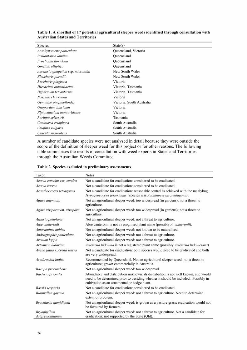
Table 1. A shortlist of 17 potential agricultural sleeper weeds identified through consultation with Australian States and Territories

Species State(s) Aeschynomene paniculata Queensland, Victoria Brillantaisia lamium Queensland Froelichia floridana Queensland Gmelina elliptica Queensland Asystasia gangetica ssp. micrantha New South Wales Eleocharis parodii New South Wales Baccharis pingraea Victoria Hieracium aurantiacum Victoria, Tasmania Hypericum tetrapterum Victoria, Tasmania Nassella charruana Victoria Oenanthe pimpinelloides Victoria, South Australia Onopordum tauricum Victoria Piptochaetium montevidense Victoria Rorippa sylvestris Tasmania Centaurea eriophora South Australia Crupina vulgaris South Australia Cuscuta suaveolens South Australia

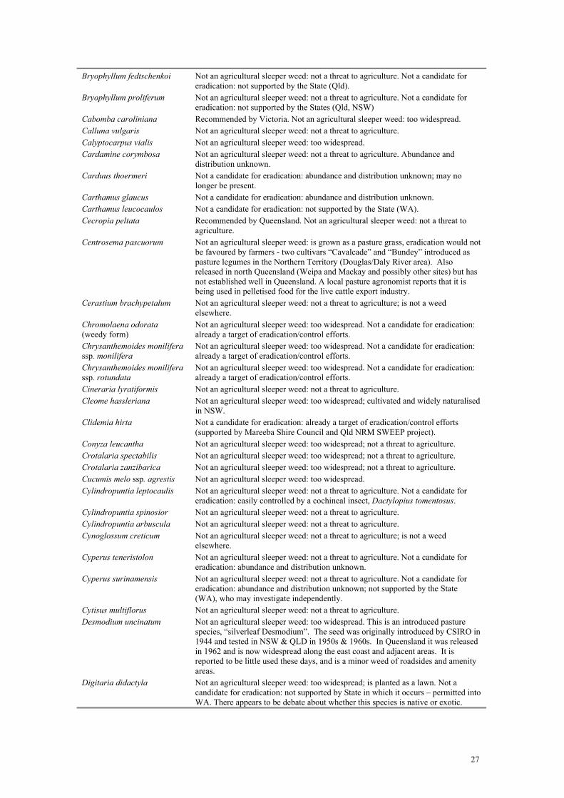
A number of candidate species were not analysed in detail because they were outside the scope of the definition of sleeper weed for this project or for other reasons. The following table summarises the results of consultation with weed experts in States and Territories through the Australian Weeds Committee.

Table 2. Species excluded in preliminary assessments

Taxon Notes Acacia catechu var. sundra Not a candidate for eradication: considered to be eradicated. Acacia karroo Not a candidate for eradication: considered to be eradicated. Acanthocereus tetragonus Not a candidate for eradication: reasonable control is achieved with the mealybug

Hypogeococcus festerianus. Species was Acanthocereus pentagonus. Agave attenuata Not an agricultural sleeper weed: too widespread (in gardens); not a threat to

agriculture. Agave vivipara var. vivapara Not an agricultural sleeper weed: too widespread (in gardens); not a threat to

agriculture. Alliaria petiolaris Not an agricultural sleeper weed: not a threat to agriculture. Aloe canteronii Aloe canteronii is not a recognised plant name (possibly A. cameronii). Amaranthus dubius Not an agricultural sleeper weed: not known to be naturalised. Andrographis paniculata Not an agricultural sleeper weed: not a threat to agriculture. Arctium lappa Not an agricultural sleeper weed: not a threat to agriculture. Artemisia ludovina Artemisia ludovina is not a registered plant name (possibly Artemisia ludoviciana). Avena fatua x Avena sativa Not a candidate for eradication: both species would need to be eradicated and both

are very widespread. Azadirachta indica Recommended by Queensland. Not an agricultural sleeper weed: not a threat to

agriculture; grown commercially in Australia. Bacopa procumbens Not an agricultural sleeper weed: too widespread. Barleria prionitis Abundance and distribution unknown: its distribution is not well known, and would

need to be determined prior to deciding whether it should be included. Possibly in cultivation as an ornamental or hedge plant.

Bassia scoparia Not a candidate for eradication: considered to be eradicated. Blainvillea gayana Not an agricultural sleeper weed: not a threat to agriculture. Need to determine

extent of problem. Brachiaria humidicola Not an agricultural sleeper weed: is grown as a pasture grass; eradication would not

be favoured by farmers. Bryophyllum daigremontianum

Not an agricultural sleeper weed: not a threat to agriculture. Not a candidate for eradication: not supported by the State (Qld).

27

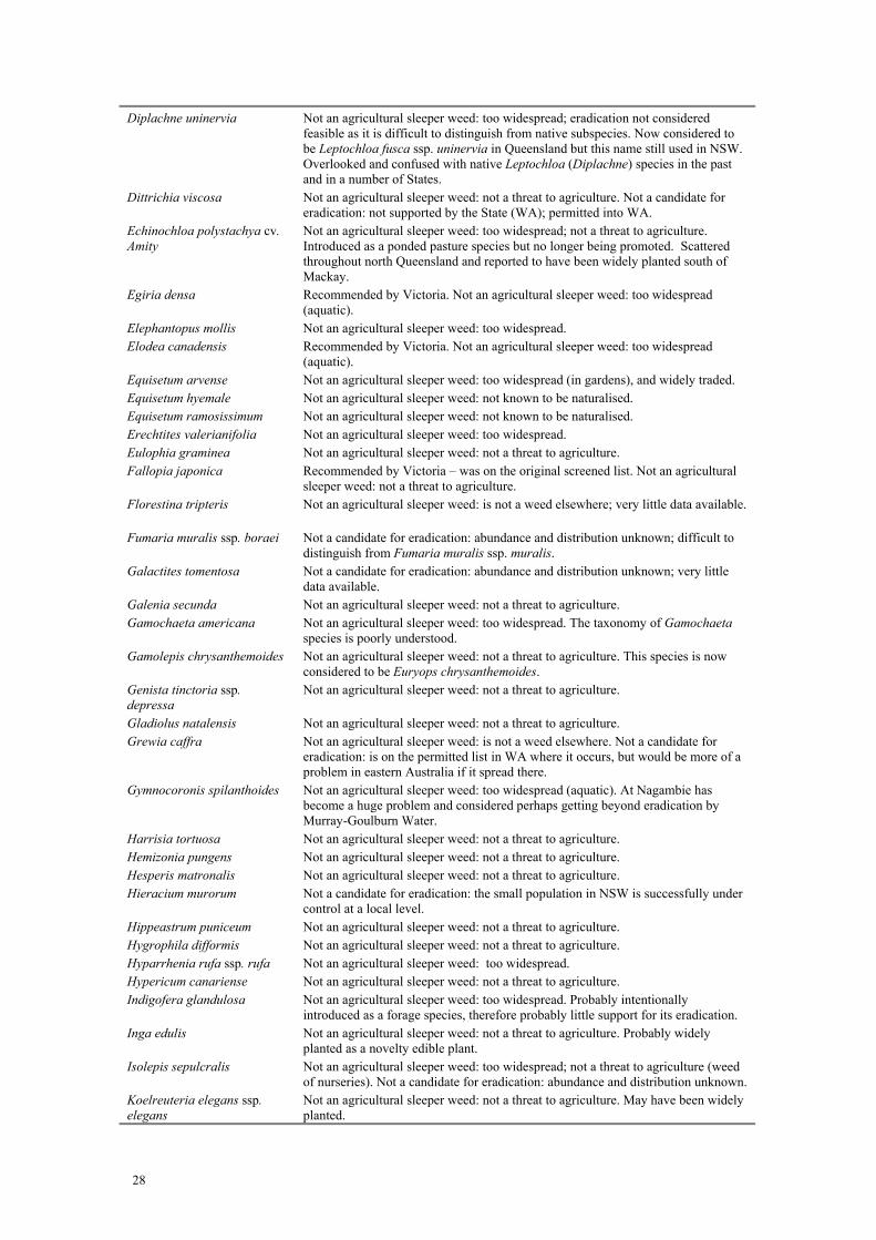
Bryophyllum fedtschenkoi Not an agricultural sleeper weed: not a threat to agriculture. Not a candidate for eradication: not supported by the State (Qld).

Bryophyllum proliferum Not an agricultural sleeper weed: not a threat to agriculture. Not a candidate for eradication: not supported by the States (Qld, NSW)

Cabomba caroliniana Recommended by Victoria. Not an agricultural sleeper weed: too widespread. Calluna vulgaris Not an agricultural sleeper weed: not a threat to agriculture. Calyptocarpus vialis Not an agricultural sleeper weed: too widespread. Cardamine corymbosa Not an agricultural sleeper weed: not a threat to agriculture. Abundance and

distribution unknown. Carduus thoermeri Not a candidate for eradication: abundance and distribution unknown; may no

longer be present. Carthamus glaucus Not a candidate for eradication: abundance and distribution unknown. Carthamus leucocaulos Not a candidate for eradication: not supported by the State (WA). Cecropia peltata Recommended by Queensland. Not an agricultural sleeper weed: not a threat to

agriculture. Centrosema pascuorum Not an agricultural sleeper weed: is grown as a pasture grass, eradication would not

be favoured by farmers - two cultivars “Cavalcade” and “Bundey” introduced as pasture legumes in the Northern Territory (Douglas/Daly River area). Also released in north Queensland (Weipa and Mackay and possibly other sites) but has not established well in Queensland. A local pasture agronomist reports that it is being used in pelletised food for the live cattle export industry.

Cerastium brachypetalum Not an agricultural sleeper weed: not a threat to agriculture; is not a weed elsewhere.

Chromolaena odorata (weedy form)

Not an agricultural sleeper weed: too widespread. Not a candidate for eradication: already a target of eradication/control efforts.

Chrysanthemoides monilifera ssp. monilifera


Chrysanthemoides monilifera ssp. rotundata


Cineraria lyratiformis Not an agricultural sleeper weed: not a threat to agriculture. Cleome hassleriana Not an agricultural sleeper weed: too widespread; cultivated and widely naturalised

in NSW. Clidemia hirta Not a candidate for eradication: already a target of eradication/control efforts

(supported by Mareeba Shire Council and Qld NRM SWEEP project). Conyza leucantha Not an agricultural sleeper weed: too widespread; not a threat to agriculture. Crotalaria spectabilis Not an agricultural sleeper weed: too widespread; not a threat to agriculture. Crotalaria zanzibarica Not an agricultural sleeper weed: too widespread; not a threat to agriculture. Cucumis melo ssp. agrestis Not an agricultural sleeper weed: too widespread. Cylindropuntia leptocaulis Not an agricultural sleeper weed: not a threat to agriculture. Not a candidate for

eradication: easily controlled by a cochineal insect, Dactylopius tomentosus. Cylindropuntia spinosior Not an agricultural sleeper weed: not a threat to agriculture. Cylindropuntia arbuscula Not an agricultural sleeper weed: not a threat to agriculture. Cynoglossum creticum Not an agricultural sleeper weed: not a threat to agriculture; is not a weed

elsewhere. Cyperus teneristolon Not an agricultural sleeper weed: not a threat to agriculture. Not a candidate for

eradication: abundance and distribution unknown. Cyperus surinamensis Not an agricultural sleeper weed: not a threat to agriculture. Not a candidate for

eradication: abundance and distribution unknown; not supported by the State (WA), who may investigate independently.

Cytisus multiflorus Not an agricultural sleeper weed: not a threat to agriculture. Desmodium uncinatum Not an agricultural sleeper weed: too widespread. This is an introduced pasture

species, “silverleaf Desmodium”. The seed was originally introduced by CSIRO in 1944 and tested in NSW & QLD in 1950s & 1960s. In Queensland it was released in 1962 and is now widespread along the east coast and adjacent areas. It is reported to be little used these days, and is a minor weed of roadsides and amenity areas.

Digitaria didactyla Not an agricultural sleeper weed: too widespread; is planted as a lawn. Not a candidate for eradication: not supported by State in which it occurs – permitted into WA. There appears to be debate about whether this species is native or exotic.

28

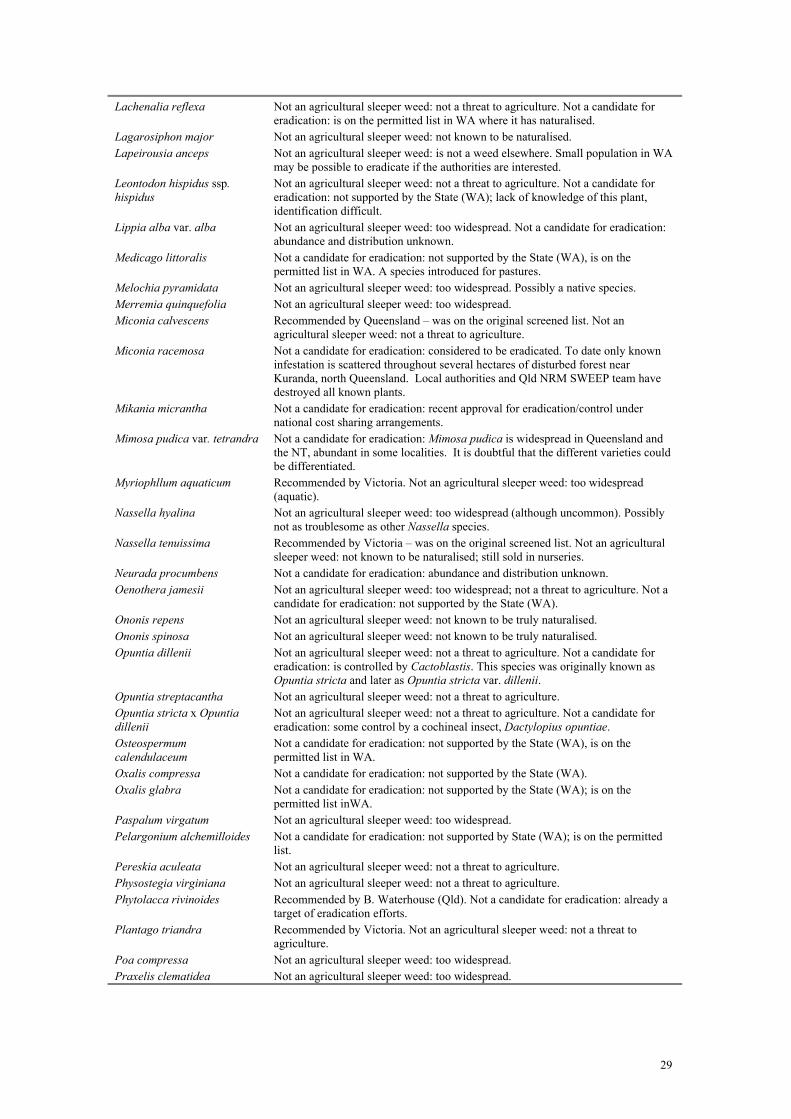
Diplachne uninervia Not an agricultural sleeper weed: too widespread; eradication not considered feasible as it is difficult to distinguish from native subspecies. Now considered to be Leptochloa fusca ssp. uninervia in Queensland but this name still used in NSW. Overlooked and confused with native Leptochloa (Diplachne) species in the past and in a number of States.

Dittrichia viscosa Not an agricultural sleeper weed: not a threat to agriculture. Not a candidate for eradication: not supported by the State (WA); permitted into WA.

Echinochloa polystachya cv. Amity

Not an agricultural sleeper weed: too widespread; not a threat to agriculture. Introduced as a ponded pasture species but no longer being promoted. Scattered throughout north Queensland and reported to have been widely planted south of Mackay.

Egiria densa Recommended by Victoria. Not an agricultural sleeper weed: too widespread (aquatic).

Elephantopus mollis Not an agricultural sleeper weed: too widespread. Elodea canadensis Recommended by Victoria. Not an agricultural sleeper weed: too widespread

(aquatic). Equisetum arvense Not an agricultural sleeper weed: too widespread (in gardens), and widely traded. Equisetum hyemale Not an agricultural sleeper weed: not known to be naturalised. Equisetum ramosissimum Not an agricultural sleeper weed: not known to be naturalised. Erechtites valerianifolia Not an agricultural sleeper weed: too widespread. Eulophia graminea Not an agricultural sleeper weed: not a threat to agriculture. Fallopia japonica Recommended by Victoria – was on the original screened list. Not an agricultural

sleeper weed: not a threat to agriculture. Florestina tripteris Not an agricultural sleeper weed: is not a weed elsewhere; very little data available.

Fumaria muralis ssp. boraei Not a candidate for eradication: abundance and distribution unknown; difficult to

distinguish from Fumaria muralis ssp. muralis. Galactites tomentosa Not a candidate for eradication: abundance and distribution unknown; very little

data available. Galenia secunda Not an agricultural sleeper weed: not a threat to agriculture. Gamochaeta americana Not an agricultural sleeper weed: too widespread. The taxonomy of Gamochaeta

species is poorly understood. Gamolepis chrysanthemoides Not an agricultural sleeper weed: not a threat to agriculture. This species is now

considered to be Euryops chrysanthemoides. Genista tinctoria ssp. depressa

Not an agricultural sleeper weed: not a threat to agriculture.

Gladiolus natalensis Not an agricultural sleeper weed: not a threat to agriculture. Grewia caffra Not an agricultural sleeper weed: is not a weed elsewhere. Not a candidate for

eradication: is on the permitted list in WA where it occurs, but would be more of a problem in eastern Australia if it spread there.

Gymnocoronis spilanthoides Not an agricultural sleeper weed: too widespread (aquatic). At Nagambie has become a huge problem and considered perhaps getting beyond eradication by Murray-Goulburn Water.

Harrisia tortuosa Not an agricultural sleeper weed: not a threat to agriculture. Hemizonia pungens Not an agricultural sleeper weed: not a threat to agriculture. Hesperis matronalis Not an agricultural sleeper weed: not a threat to agriculture. Hieracium murorum Not a candidate for eradication: the small population in NSW is successfully under

control at a local level. Hippeastrum puniceum Not an agricultural sleeper weed: not a threat to agriculture. Hygrophila difformis Not an agricultural sleeper weed: not a threat to agriculture. Hyparrhenia rufa ssp. rufa Not an agricultural sleeper weed: too widespread. Hypericum canariense Not an agricultural sleeper weed: not a threat to agriculture. Indigofera glandulosa Not an agricultural sleeper weed: too widespread. Probably intentionally

introduced as a forage species, therefore probably little support for its eradication. Inga edulis Not an agricultural sleeper weed: not a threat to agriculture. Probably widely

planted as a novelty edible plant. Isolepis sepulcralis Not an agricultural sleeper weed: too widespread; not a threat to agriculture (weed

of nurseries). Not a candidate for eradication: abundance and distribution unknown. Koelreuteria elegans ssp. elegans

Not an agricultural sleeper weed: not a threat to agriculture. May have been widely planted.

29

Lachenalia reflexa Not an agricultural sleeper weed: not a threat to agriculture. Not a candidate for eradication: is on the permitted list in WA where it has naturalised.

Lagarosiphon major Not an agricultural sleeper weed: not known to be naturalised. Lapeirousia anceps Not an agricultural sleeper weed: is not a weed elsewhere. Small population in WA

may be possible to eradicate if the authorities are interested. Leontodon hispidus ssp. hispidus

Not an agricultural sleeper weed: not a threat to agriculture. Not a candidate for eradication: not supported by the State (WA); lack of knowledge of this plant, identification difficult.

Lippia alba var. alba Not an agricultural sleeper weed: too widespread. Not a candidate for eradication: abundance and distribution unknown.

Medicago littoralis Not a candidate for eradication: not supported by the State (WA), is on the permitted list in WA. A species introduced for pastures.

Melochia pyramidata Not an agricultural sleeper weed: too widespread. Possibly a native species. Merremia quinquefolia Not an agricultural sleeper weed: too widespread. Miconia calvescens Recommended by Queensland – was on the original screened list. Not an

agricultural sleeper weed: not a threat to agriculture. Miconia racemosa Not a candidate for eradication: considered to be eradicated. To date only known

infestation is scattered throughout several hectares of disturbed forest near Kuranda, north Queensland. Local authorities and Qld NRM SWEEP team have destroyed all known plants.

Mikania micrantha Not a candidate for eradication: recent approval for eradication/control under national cost sharing arrangements.

Mimosa pudica var. tetrandra Not a candidate for eradication: Mimosa pudica is widespread in Queensland and the NT, abundant in some localities. It is doubtful that the different varieties could be differentiated.

Myriophllum aquaticum Recommended by Victoria. Not an agricultural sleeper weed: too widespread (aquatic).

Nassella hyalina Not an agricultural sleeper weed: too widespread (although uncommon). Possibly not as troublesome as other Nassella species.

Nassella tenuissima Recommended by Victoria – was on the original screened list. Not an agricultural sleeper weed: not known to be naturalised; still sold in nurseries.

Neurada procumbens Not a candidate for eradication: abundance and distribution unknown. Oenothera jamesii Not an agricultural sleeper weed: too widespread; not a threat to agriculture. Not a

candidate for eradication: not supported by the State (WA). Ononis repens Not an agricultural sleeper weed: not known to be truly naturalised. Ononis spinosa Not an agricultural sleeper weed: not known to be truly naturalised. Opuntia dillenii Not an agricultural sleeper weed: not a threat to agriculture. Not a candidate for

eradication: is controlled by Cactoblastis. This species was originally known as Opuntia stricta and later as Opuntia stricta var. dillenii.

Opuntia streptacantha Not an agricultural sleeper weed: not a threat to agriculture. Opuntia stricta x Opuntia dillenii

Not an agricultural sleeper weed: not a threat to agriculture. Not a candidate for eradication: some control by a cochineal insect, Dactylopius opuntiae.

Osteospermum calendulaceum

Not a candidate for eradication: not supported by the State (WA), is on the permitted list in WA.

Oxalis compressa Not a candidate for eradication: not supported by the State (WA). Oxalis glabra Not a candidate for eradication: not supported by the State (WA); is on the

permitted list inWA. Paspalum virgatum Not an agricultural sleeper weed: too widespread. Pelargonium alchemilloides Not a candidate for eradication: not supported by State (WA); is on the permitted

list. Pereskia aculeata Not an agricultural sleeper weed: not a threat to agriculture. Physostegia virginiana Not an agricultural sleeper weed: not a threat to agriculture. Phytolacca rivinoides Recommended by B. Waterhouse (Qld). Not a candidate for eradication: already a

target of eradication efforts. Plantago triandra Recommended by Victoria. Not an agricultural sleeper weed: not a threat to

agriculture. Poa compressa Not an agricultural sleeper weed: too widespread. Praxelis clematidea Not an agricultural sleeper weed: too widespread.

30

Proboscidea louisianica ssp. fragrans

Not an agricultural sleeper weed: not a threat to agriculture. Not a candidate for eradication: difficult to distinguish from Proboscidea lousianica ssp. louisianica and Ibicella lutea when not in flower.

Quisqualis indica Not an agricultural sleeper weed: not known to be truly naturalised. Planted as an ornamental.

Retama raetam Not an agricultural sleeper weed: not a threat to agriculture. Not a candidate for eradication: not supported by the State (WA).

Rhaphiolepis umbellata Not an agricultural sleeper weed: not a threat to agriculture; too widespread (in gardens).

Rhizophora mangle Recommended by Queensland. Not an agricultural sleeper weed: marine species are not within the scope of this project.

Rhodomyrtus tomentosa Not an agricultural sleeper weed: not known to be naturalised. Appears to have been introduced and cultivated as an unusual tropical fruit – still sold in nurseries.

Richardia stellaris Not an agricultural sleeper weed: too widespread. Rubus alceifolius Not an agricultural sleeper weed: too widespread. Difficult to distinguish from the

native species R. moluccanus which occupies the same range. Sagittaria graminea Recommended by Victoria. Not an agricultural sleeper weed: too widespread

(aquatic). Senecio glastifolius Not an agricultural sleeper weed: not a threat to agriculture; too widespread. Senna septemtrionalis Not an agricultural sleeper weed: too widespread. Setaria sphacelata var. splendida

Not an agricultural sleeper weed: too widespread. Not a candidate for eradication: grown as a pasture species; difficult to distinguish from the more widespread S. sphacelata var. sericea.

Solanum capsicoides Not an agricultural sleeper weed: not a threat to agriculture; too widespread. Solanum retroflexum Not an agricultural sleeper weed: not a threat to agriculture. Not a candidate for

eradication: abundance and distribution unknown. Solanum villosum Not a candidate for eradication: abundance and distribution unknown. Spergula pentandra Not an agricultural sleeper weed: not a threat to agriculture; too widespread. Stevia eupatoria Not a candidate for eradication: considered to be eradicated. Stipa gigantidis Is not a registered plant name (possibly S. gigantea or S. gigantica). Tephrosia nana Not an agricultural sleeper weed: not a threat to agriculture; very little data

available. Thunbergia alata Not an agricultural sleeper weed: too widespread. Thunbergia grandiflora Not an agricultural sleeper weed: not a threat to agriculture; too widespread (in

gardens). Thunbergia laurifolia Not an agricultural sleeper weed: not a threat to agriculture; too widespread (in

gardens). Tipuana tipu Not an agricultural sleeper weed: not a threat to agriculture; too widespread (in

gardens). Trianoptiles solitaria Not an agricultural sleeper weed: not a threat to agriculture. Trifolium fragiferum var. pulchellum

Not an agricultural sleeper weed: introduced as a pasture species.

Vicia sativa ssp. cordata Not an agricultural sleeper weed: introduced as a pasture species.

References Groves, R.H., Hosking, J.R., Cooke, D.A., Johnson, R.W., Lepschi, B.J., Mitchell, A.A.,

Moerkerk, M., Randall, R.P., Rozefelds, A.C. and Waterhouse, B.M. (2002) The naturalised non-native flora of Australia: its categorisation and threat to agricultural ecosystems. Report to the Bureau of Rural Sciences, Canberra.

NHT (2003) National Weeds Program. National Heritage Trust (NHT), Environment Australia. www.nht.gov.au/funding/applications/weeds.html

Nothrop, L. and Cunningham, D. (2003) BRS project: Investigations and strategic control of agricultural "sleeper weeds". Out of session agenda paper. Australian Weeds Committee, Australia.

31

Appendix B. Desktop research methods

Books and previous reports Brinkley, T. and Bomford, M. (2002). ‘Agricultural Sleeper Weeds in Australia. What is the

potential threat?’ Bureau of Rural Sciences, Canberra.

Auld, B.A. and Medd, R.W. (1987). ‘Weeds: An illustrated botanical guide to the weeds of Australia’. (Inkata Press, Melbourne).

Curhes, S. and Edwards, R. (1998). ‘Potential Environmental Weeds in Australia: Candidate Species for Preventative Control’. (Biodiversity Group, Environment Australia, Canberra).

Groves, R.H. and Hosking, J.R. (1998). ‘Recent Incursions of Weeds to Australia 1971-1995’. Technical series no. 3, (CRC for Weed Management Systems, Australia).

Groves, R.H., Hosking, J.R., Cooke, D.A., Johnson, R.W. Lepschi, B.J., Mitchell, A.A., Moerkerk, M., Randall, R.P., Rozefelds, A.C. and Waterhouse, B.M. (2002). ‘The naturalised non-native flora of Australia: its categorisation and threat to agricultural ecosystems’. (Bureau of Rural Sciences, Canberra).

Groves, R.H., Hosking, J.R., Batianoff, G.N., Cooke, D.A., Cowie, I.D., Keighery, G.J., Lepschi, B.J., Rozefelds, A.C., and Walsh, N.G. (2000). ‘The naturalised non-native flora of Australia: its categorisation and threat to native plant biodiversity’. (Environment Australia, Canberra).

Lamp, C. and Collet, F. (1993). ‘Field guide to weeds in Australia’. (Inkata Press, Melbourne).

Longmore, R. (ed.) (1991). ‘Plant invasions: The incidence of environmental weeds in Australia’ 2. (Australian National Parks and Wildlife Service, Canberra).

Parsons, W.T. and Cuthbertson, E.G. (1992) ‘Noxious Weeds of Australia’. (Inkata Press, Melbourne).

Randall, R.P. (2002). ‘A Global Compendium of Weeds’. (R.G. and F.J. Richardson, Melbourne)

Internet sites and databases

In addition to general internet search engines, the following internet sites and databases were searched for information relating to each weed species on the draft candidate list.

ANH, CPBR (2002) Australia’s Virtual Herbarium. Centre for Plant Biodiversity Research (CPBR), Australian National Herbarium (ANH). www.cpbr.gov.au/avh/

Baldwin, B.G., Boyd, S., Ertter, B.J., Patterson, R.W., Rosatti, T.J. and Wilken D.H. (eds) (2002) UC/JEPS specimen database (SMASCH), Jepson Online Interchange. Jepson Herbaria, University of California. ucjeps.berkeley.edu/interchange.html

Botany.Com (2002) Botany.Com website. www.botany.com/

CABI Publishing (2002) PEST CABweb. CABI Publishing, CAB International. pest.cabweb.org/

CDFA (2001). Encycloweedia: Notes on Identification, Biology, and Management of Plants Defined as Noxious Weeds by California Law, Plant Health and Pest Prevention Services, California Department of Food and Agriculture (CDFA). http://pi.cdfa.ca.gov/weedinfo/Index.html

32

IPK (2002) Mansfeld's World Database of Agricultural and Horticultural Crops. Institute of Plant Genetics and Crop Plant Research (IPK), Gatersleben. mansfeld.ipk-gatersleben.de/Mansfeld/

ILDIS (2001) LegumeWeb Version 6.06. International Legume Database & Information Service (ILDIS), United Kingdom. www.ildis.org/LegumeWeb/

Missouri Botanical Gardens (2002 onwards) W3Tropicos. [VAST (VAScular Tropicos) nomenclatural database] Missouri Botanical Gardens. mobot.mobot.org/W3T/Search/vast.html

NHT (2003) Weeds Australia. National Weeds Strategy, National Heritage Trust (NHT). search.weeds.org.au/

RBGK, HUH and ANH (1999) International Plant Names Index. The Plant Names Project. The Royal Botanic Gardens Kew (RBGK), The Harvard University Herbaria (HUH) and the Australian National Herbarium (ANH). www.ipni.org/index.html

UC, DBPS (2000 - 2002) Plant Biology Index. Department of Botany and Plant Sciences (DBPS), University of California (UC), Riverside. plant.ucr.edu/

UH and USGS, BRD (2002). Information Index for Selected Alien Plants in Hawaii. Hawaiian Ecosystems at Risk (HEAR) Project, Botany Department, University of Hawaii and the Biological Resources Division, United States Geological Survey. www.hear.org/AlienSpeciesInHawaii/InfoIndexPlants.htm

USDA, ARS (1997 - 2003) Noxious Weeds in the US and Canada. Invaders Database System Agricultural Research Service (ARS), United States Department of Agriculture (USDA). invader.dbs.umt.edu/Noxious_Weeds/

USDA, ARS (2002) Germplasm Resources Information Network (GRIN) Taxonomy. National Genetic Resources Program, National Germplasm Resources Laboratory, Agricultural Research Service (ARS), United States Department of Agriculture (USDA), Beltsville, Maryland. www.ars-grin.gov/npgs/tax/index.html

USDA, IPIF (2002) Plant Threats to Pacific Ecosystems Version 3.3. Pacific Islands Ecosystems at Risk (PIER) Project, Institute of Pacific Islands Forestry (IPIF), United States Department of Agriculture (USDA). www.hear.org/pier/threats.htm

USDA, NRCS (2003) PLANTS Database Version 3.5. Natural Resources Conservation Service (NRCS), United States Department of Agriculture (USDA), Baton Rouge, Los Angeles. plants.usda.gov/index.html

Watson, L. and Dallwitz, M.J. (1992 onwards). ‘Grass Genera of the World: Descriptions, Illustrations, Identification, and Information Retrieval; including Synonyms, Morphology, Anatomy, Physiology, Phytochemistry, Cytology, Classification, Pathogens, World and Local Distribution, and References.’ biodiversity.uno.edu/delta/grass/index.htm

Literature databases

The following electronic databases were searched for journal articles and other published material referring to each weed species on the draft candidate list.

AGRICOLA: 1979 – December 2002.

AGNR: ABOA (Agriculture).

AGNR: ARRIP (Rural Research in Progress).

AGNR: CARRP (Rural Research Completed).

33

AGNR: STREAMLINE (Natural resources).

CAB Abstracts: 1972 – July 2002.

HERIT: ELIXIR (Natural resources, Environment).

General Science Plus. 80-proquest.umi.com.virtual.anu.edu.au/pqdweb?RQT=306&TS=1044231840

Ingenta: Index to Worldwide Periodical Literature (UnCover Plus.) 80-www.ingenta.com.virtual.anu.edu.au/

Science Direct (Via ElsevierScience, copyright 2002). 80-www.sciencedirect.com.virtual.anu.edu.au/

Web of Science. 80-isi0.isiknowledge.com.virtual.anu.edu.au/portal.cgi/wos

34

Appendix C. Distribution maps and potential impact assessments

Climate matching Climate is considered to be the most important factor in determining the potential distribution of a plant species. Where there is little experimental data on climatic preferences of a plant, weed scientists generally rely on simple models where the input is based on where the plant is known to grow at present and the output is an extrapolation of this in the new environment.

For the 17 candidate species, we assessed the match of climate between extra-Australian occurrences and areas within Australia. We used the climate-modelling program ‘Climate’ (Pheloung 1996) with the same statistical approach that applied to the determination of Weeds of National Significance. The cumulative analysis with the closest Euclidian match was used to identify areas within a Euclidian distance of 0 to 20 (on an arbitrary scale of 0 to 100) (after Thorp and Lynch 2000; Duncan et al. 2001; Kriticos and Randall 2001).

Overseas distribution data including the native and naturalised range of each weed was compiled from various sources listed in Appendix C, which lists each taxon’s distribution, both native and naturalised, and any other data that was considered in the predictions together with maps of the current and potential distribution in Australia. The majority of the input data was at a coarse resolution, i.e. country or part of country. Where information was available, the overseas distribution was refined using an Atlas (Macquarie 1994) and climate zone maps (e.g. Seedland 1999). In cases where a species is reportedly limited by elevation, this information was used by removing higher elevation stations from the Climate analysis. For the one aquatic species, the potential distribution was modelled using temperature parameters only.

Climate and Climex often produce different outputs for a species based on the same inputs, e.g. Kritcos and Randall (2001). The predicted distribution for B. lamium in this report (Climate) differs from an earlier prediction based on Climex (Brinkley and Bomford 2002). This difference is similar to those reported by Kriticos and Randall (2001) and other papers comparing the output of Climate and Climex. This kind of discrepancy highlights the need for further refinement of Climate matching models used for Weed Risk Assessment. Nevertheless, Climate provides a useful prediction at the broad national scale required for this type of analysis.

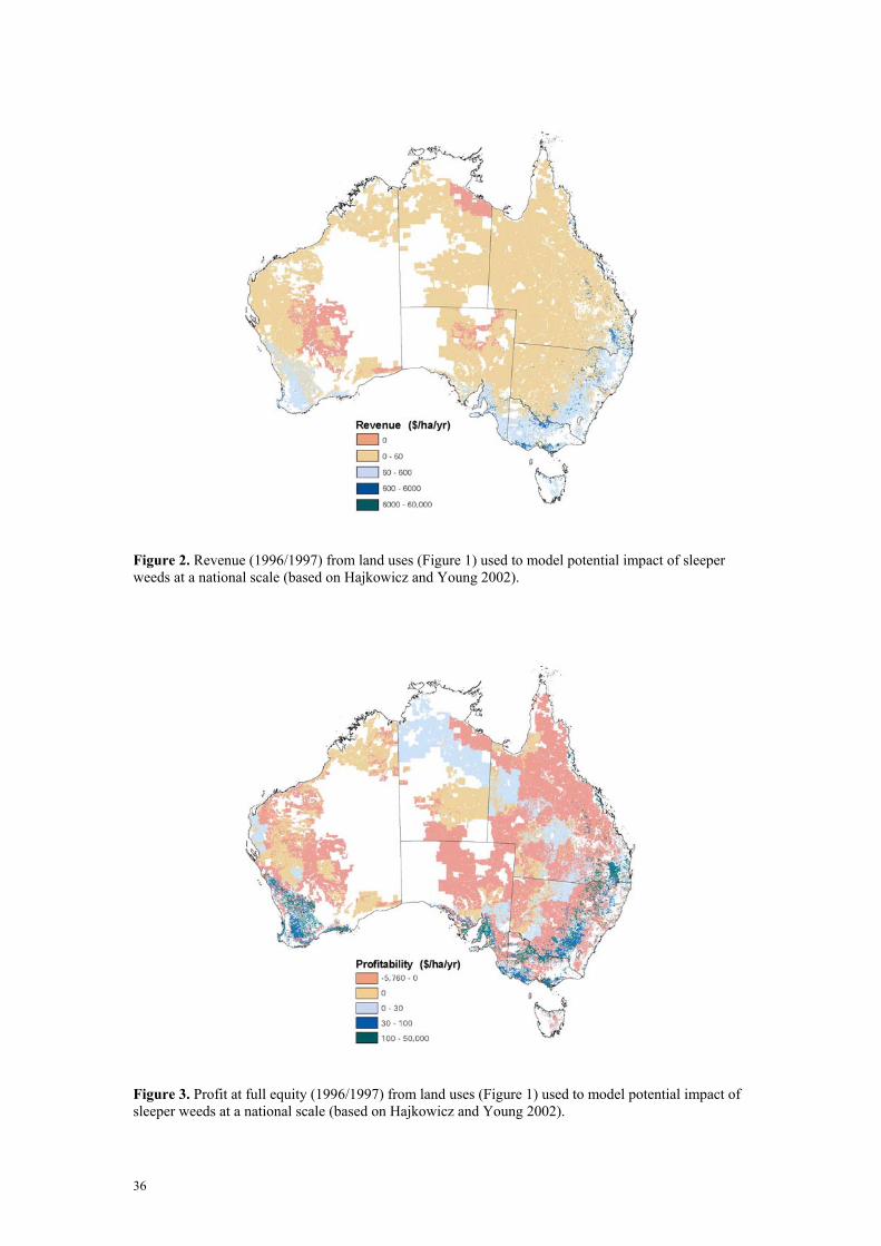
Land use matching and value of production at risk The climate matching method gives an output that defines the area potentially suitable for a plant in Australia, based on its climate profile. Brinkley and Bomford (2002) took this approach one step further and quantified the area of agricultural land that could potentially be impacted on by a weed, and the value of production potentially at risk based on land use. For example, the potential impact of a weed of pastures is measured only in terms of grazing land that is climatically suitable, not all land.

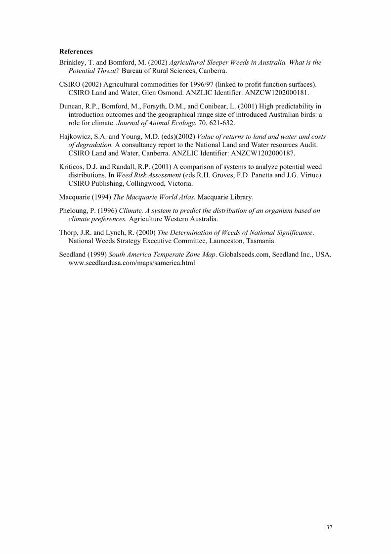
For the purposes of this study, we assessed the magnitude of the potential impact of a weed by quantifying both the value of production (revenue) and the profit at full equity (PFE) of the land use(s) potentially at risk within the potential distribution predicted by climate matching. The other key difference between our approach and that of Brinkley and Bomford (2002) is that we used Climate instead of Climex as described above.

35

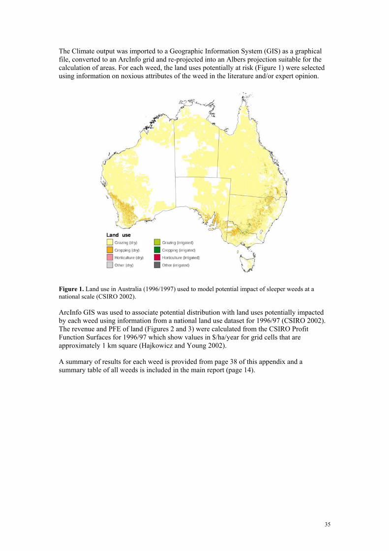
The Climate output was imported to a Geographic Information System (GIS) as a graphical file, converted to an ArcInfo grid and re-projected into an Albers projection suitable for the calculation of areas. For each weed, the land uses potentially at risk (Figure 1) were selected using information on noxious attributes of the weed in the literature and/or expert opinion.

Figure 1. Land use in Australia (1996/1997) used to model potential impact of sleeper weeds at a national scale (CSIRO 2002).

ArcInfo GIS was used to associate potential distribution with land uses potentially impacted by each weed using information from a national land use dataset for 1996/97 (CSIRO 2002). The revenue and PFE of land (Figures 2 and 3) were calculated from the CSIRO Profit Function Surfaces for 1996/97 which show values in $/ha/year for grid cells that are approximately 1 km square (Hajkowicz and Young 2002).

A summary of results for each weed is provided from page 38 of this appendix and a summary table of all weeds is included in the main report (page 14).

36

Figure 2. Revenue (1996/1997) from land uses (Figure 1) used to model potential impact of sleeper weeds at a national scale (based on Hajkowicz and Young 2002).

Figure 3. Profit at full equity (1996/1997) from land uses (Figure 1) used to model potential impact of sleeper weeds at a national scale (based on Hajkowicz and Young 2002).

37

References Brinkley, T. and Bomford, M. (2002) Agricultural Sleeper Weeds in Australia. What is the

Potential Threat? Bureau of Rural Sciences, Canberra.

CSIRO (2002) Agricultural commodities for 1996/97 (linked to profit function surfaces). CSIRO Land and Water, Glen Osmond. ANZLIC Identifier: ANZCW1202000181.

Duncan, R.P., Bomford, M., Forsyth, D.M., and Conibear, L. (2001) High predictability in introduction outcomes and the geographical range size of introduced Australian birds: a role for climate. Journal of Animal Ecology, 70, 621-632.

Hajkowicz, S.A. and Young, M.D. (eds)(2002) Value of returns to land and water and costs of degradation. A consultancy report to the National Land and Water resources Audit. CSIRO Land and Water, Canberra. ANZLIC Identifier: ANZCW1202000187.

Kriticos, D.J. and Randall, R.P. (2001) A comparison of systems to analyze potential weed distributions. In Weed Risk Assessment (eds R.H. Groves, F.D. Panetta and J.G. Virtue). CSIRO Publishing, Collingwood, Victoria.

Macquarie (1994) The Macquarie World Atlas. Macquarie Library.

Pheloung, P. (1996) Climate. A system to predict the distribution of an organism based on climate preferences. Agriculture Western Australia.

Thorp, J.R. and Lynch, R. (2000) The Determination of Weeds of National Significance. National Weeds Strategy Executive Committee, Launceston, Tasmania.

Seedland (1999) South America Temperate Zone Map. Globalseeds.com, Seedland Inc., USA. www.seedlandusa.com/maps/samerica.html

38

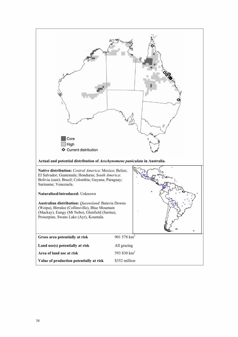
Actual and potential distribution of Aeschynomene paniculata in Australia.

Native distribution: Central America: Mexico; Belize; El Salvador; Guatemala; Honduras; South America: Bolivia (east); Brazil; Colombia; Guyana; Paraguay; Suriname; Venezuela.

Naturalised/introduced: Unknown

Australian distribution: Queensland: Batavia Downs (Weipa), Birralee (Collinsville), Blue Mountain (Mackay), Eungy (Mt Nebo), Glenfield (Sarina), Proserpine, Swans Lake (Ayr), Koumala.

Gross area potentially at risk 901 578 km2

Land use(s) potentially at risk All grazing

Area of land use at risk 593 830 km2

Value of production potentially at risk $352 million

p

39

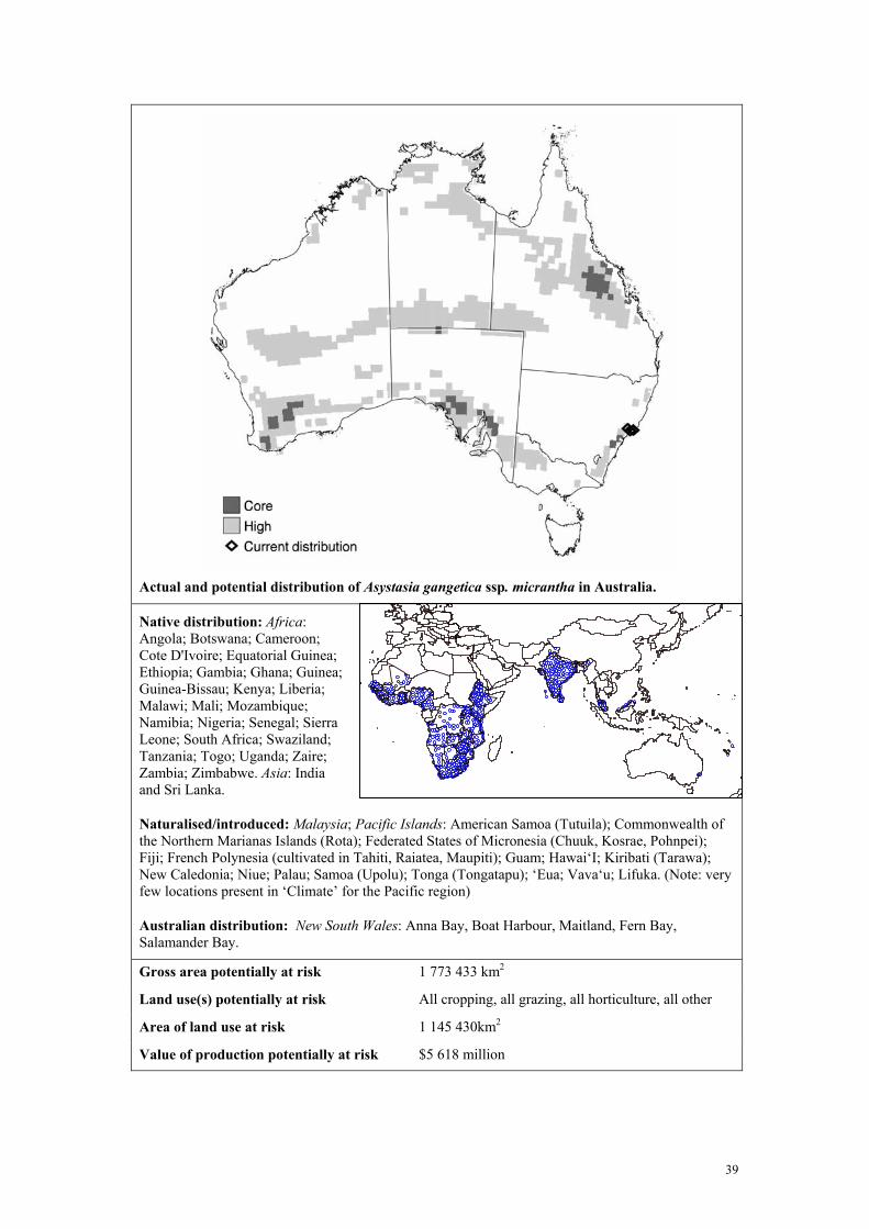
Actual and potential distribution of Asystasia gangetica ssp. micrantha in Australia.

Native distribution: Africa: Angola; Botswana; Cameroon; Cote D'Ivoire; Equatorial Guinea; Ethiopia; Gambia; Ghana; Guinea; Guinea-Bissau; Kenya; Liberia; Malawi; Mali; Mozambique; Namibia; Nigeria; Senegal; Sierra Leone; South Africa; Swaziland; Tanzania; Togo; Uganda; Zaire; Zambia; Zimbabwe. Asia: India and Sri Lanka.

Naturalised/introduced: Malaysia; Pacific Islands: American Samoa (Tutuila); Commonwealth of the Northern Marianas Islands (Rota); Federated States of Micronesia (Chuuk, Kosrae, Pohnpei); Fiji; French Polynesia (cultivated in Tahiti, Raiatea, Maupiti); Guam; Hawai‘I; Kiribati (Tarawa); New Caledonia; Niue; Palau; Samoa (Upolu); Tonga (Tongatapu); ‘Eua; Vava‘u; Lifuka. (Note: very few locations present in ‘Climate’ for the Pacific region)

Australian distribution: New South Wales: Anna Bay, Boat Harbour, Maitland, Fern Bay, Salamander Bay.

Gross area potentially at risk 1 773 433 km2

Land use(s) potentially at risk All cropping, all grazing, all horticulture, all other

Area of land use at risk 1 145 430km2

Value of production potentially at risk $5 618 million

40

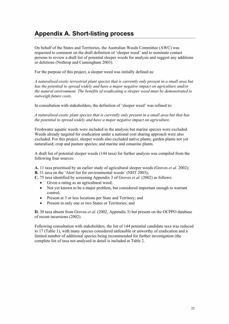
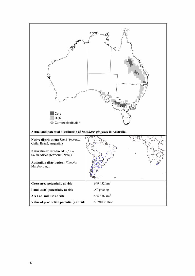
Actual and potential distribution of Baccharis pingraea in Australia.

Native distribution: South America: Chile; Brazil; Argentina

Naturalised/introduced: Africa: South Africa (KwaZulu-Natal).

Australian distribution: Victoria: Maryborough.





_ p

41

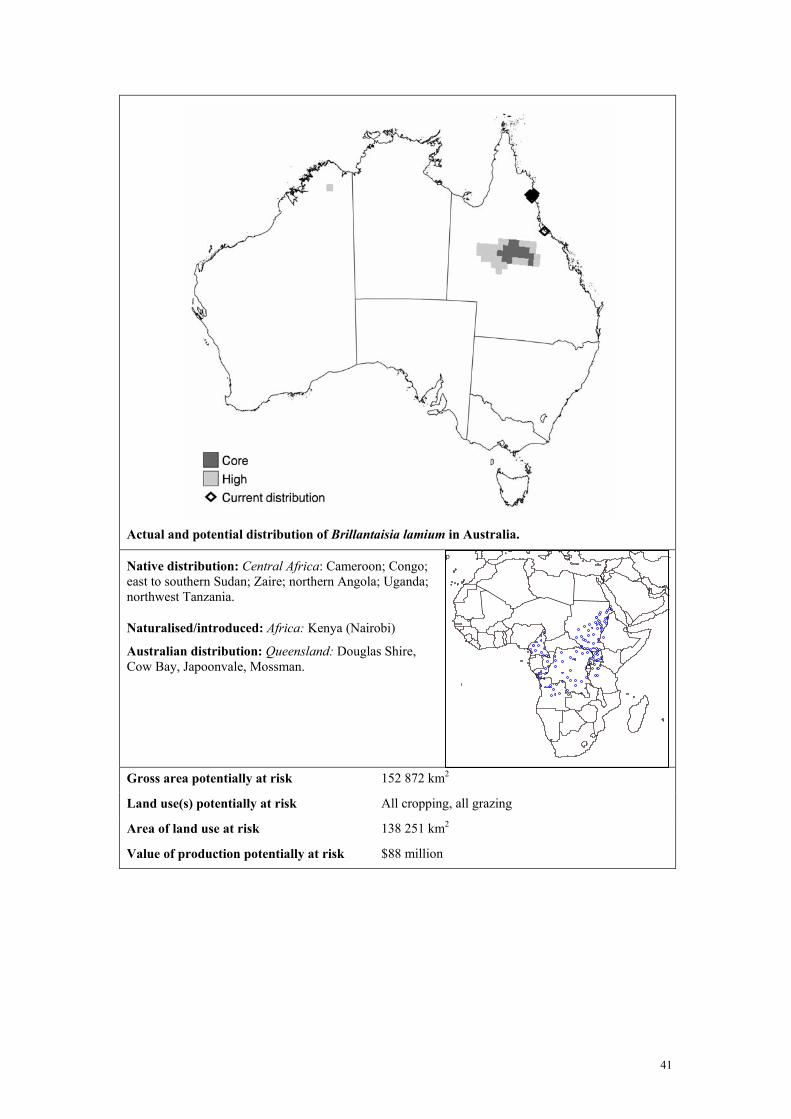
Actual and potential distribution of Brillantaisia lamium in Australia.

Native distribution: Central Africa: Cameroon; Congo; east to southern Sudan; Zaire; northern Angola; Uganda; northwest Tanzania.

Naturalised/introduced: Africa: Kenya (Nairobi)

Australian distribution: Queensland: Douglas Shire, Cow Bay, Japoonvale, Mossman.


Land use(s) potentially at risk All cropping, all grazing



p

42

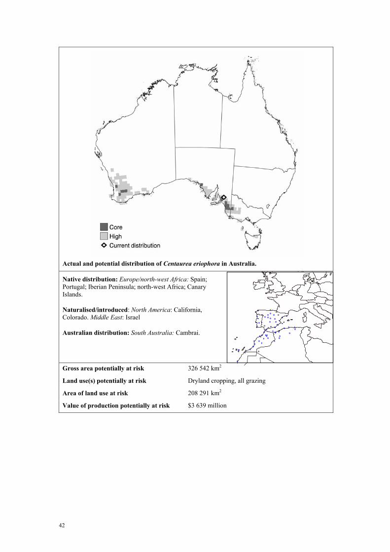
Actual and potential distribution of Centaurea eriophora in Australia.

Native distribution: Europe/north-west Africa: Spain; Portugal; Iberian Peninsula; north-west Africa; Canary Islands.

Naturalised/introduced: North America: California, Colorado. Middle East: Israel

Australian distribution: South Australia: Cambrai.


Land use(s) potentially at risk Dryland cropping, all grazing



43

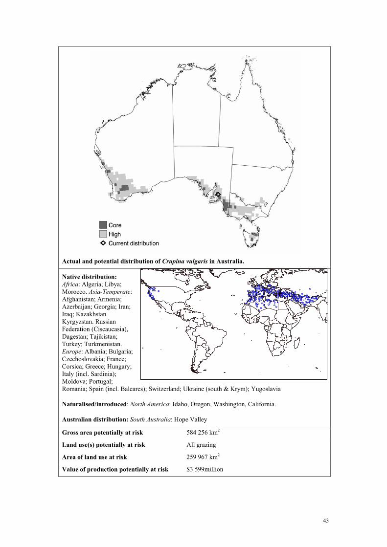
Actual and potential distribution of Crupina vulgaris in Australia.

Native distribution: Africa: Algeria; Libya; Morocco. Asia-Temperate: Afghanistan; Armenia; Azerbaijan; Georgia; Iran; Iraq; Kazakhstan Kyrgyzstan. Russian Federation (Ciscaucasia), Dagestan; Tajikistan; Turkey; Turkmenistan. Europe: Albania; Bulgaria; Czechoslovakia; France; Corsica; Greece; Hungary; Italy (incl. Sardinia); Moldova; Portugal; Romania; Spain (incl. Baleares); Switzerland; Ukraine (south & Krym); Yugoslavia

Naturalised/introduced: North America: Idaho, Oregon, Washington, California.

Australian distribution: South Australia: Hope Valley




Value of production potentially at risk $3 599million

44

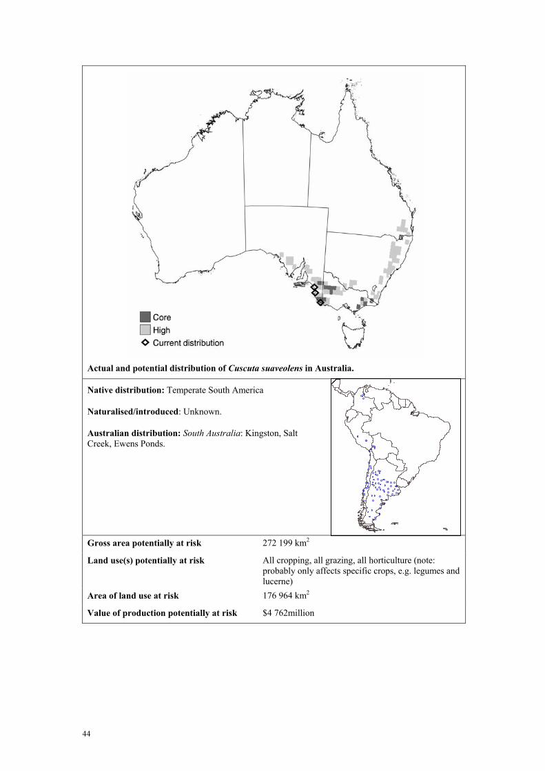
Actual and potential distribution of Cuscuta suaveolens in Australia.

Native distribution: Temperate South America

Naturalised/introduced: Unknown.

Australian distribution: South Australia: Kingston, Salt Creek, Ewens Ponds.


Land use(s) potentially at risk All cropping, all grazing, all horticulture (note: probably only affects specific crops, e.g. legumes and lucerne)



45

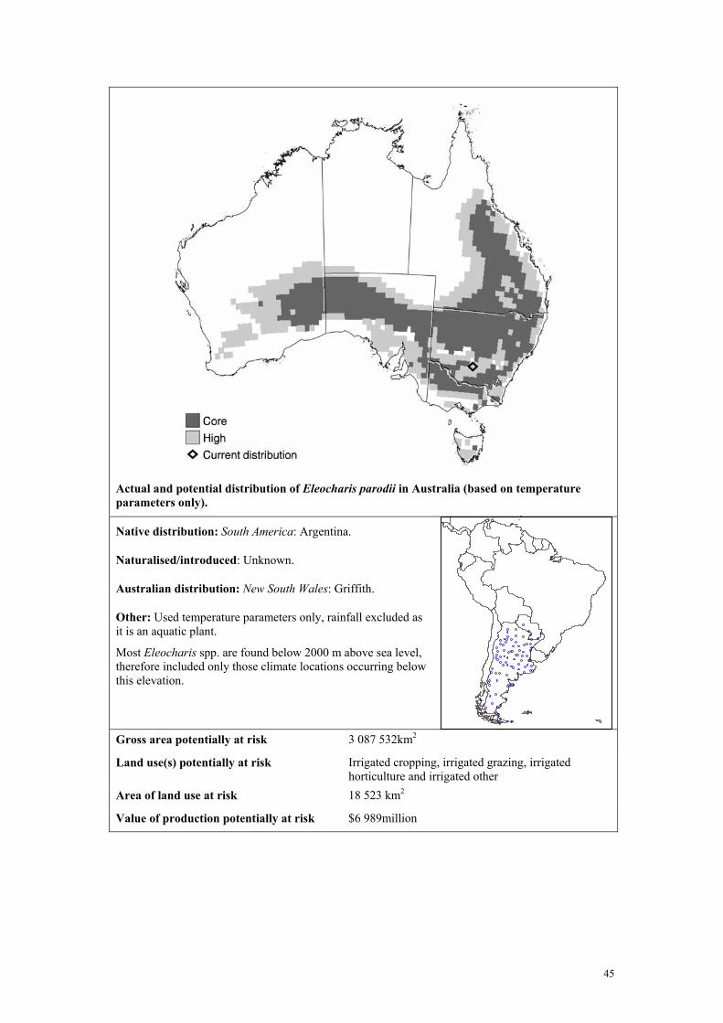
Actual and potential distribution of Eleocharis parodii in Australia (based on temperature parameters only).

Native distribution: South America: Argentina.


Australian distribution: New South Wales: Griffith.

Other: Used temperature parameters only, rainfall excluded as it is an aquatic plant.

Most Eleocharis spp. are found below 2000 m above sea level, therefore included only those climate locations occurring below this elevation.

Gross area potentially at risk 3 087 532km2

Land use(s) potentially at risk Irrigated cropping, irrigated grazing, irrigated horticulture and irrigated other



46

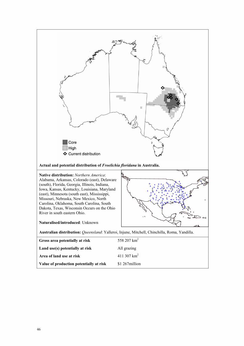
Actual and potential distribution of Froelichia floridana in Australia.

Native distribution: Northern America: Alabama, Arkansas, Colorado (east), Delaware (south), Florida, Georgia, Illinois, Indiana, Iowa, Kansas, Kentucky, Louisiana, Maryland (east), Minnesota (south east), Mississippi, Missouri, Nebraska, New Mexico, North Carolina, Oklahoma, South Carolina, South Dakota, Texas, Wisconsin Occurs on the Ohio River in south eastern Ohio.

Naturalised/introduced: Unknown

Australian distribution: Queensland: Yalleroi, Injune, Mitchell, Chinchilla, Roma, Yandilla.





47

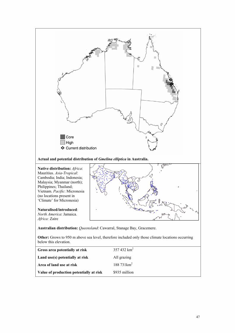
Actual and potential distribution of Gmelina elliptica in Australia.

Native distribution: Africa: Mauritius. Asia-Tropical: Cambodia; India; Indonesia; Malaysia; Myanmar (north); Philippines; Thailand; Vietnam. Pacific: Micronesia (no locations present in ‘Climate’ for Micronesia)

Naturalised/introduced: North America: Jamaica. Africa: Zaire

Australian distribution: Queensland: Cawarral, Stanage Bay, Gracemere.

Other: Grows to 950 m above sea level, therefore included only those climate locations occurring below this elevation.



Area of land use at risk 188 731km2


48

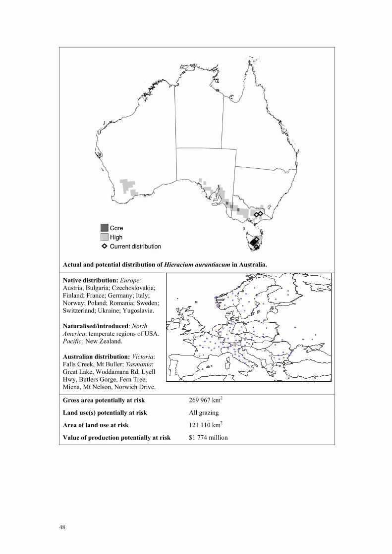
Actual and potential distribution of Hieracium aurantiacum in Australia.

Native distribution: Europe: Austria; Bulgaria; Czechoslovakia; Finland; France; Germany; Italy; Norway; Poland; Romania; Sweden; Switzerland; Ukraine; Yugoslavia.

Naturalised/introduced: North America: temperate regions of USA. Pacific: New Zealand.

Australian distribution: Victoria: Falls Creek, Mt Buller; Tasmania: Great Lake, Woddamana Rd, Lyell Hwy, Butlers Gorge, Fern Tree, Miena, Mt Nelson, Norwich Drive.





49

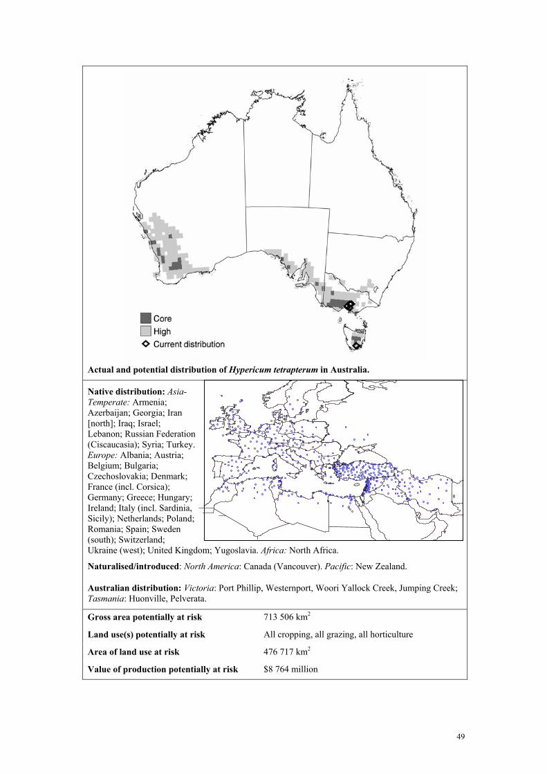
Actual and potential distribution of Hypericum tetrapterum in Australia.

Native distribution: Asia-Temperate: Armenia; Azerbaijan; Georgia; Iran [north]; Iraq; Israel; Lebanon; Russian Federation (Ciscaucasia); Syria; Turkey. Europe: Albania; Austria; Belgium; Bulgaria; Czechoslovakia; Denmark; France (incl. Corsica); Germany; Greece; Hungary; Ireland; Italy (incl. Sardinia, Sicily); Netherlands; Poland; Romania; Spain; Sweden (south); Switzerland; Ukraine (west); United Kingdom; Yugoslavia. Africa: North Africa.

Naturalised/introduced: North America: Canada (Vancouver). Pacific: New Zealand.

Australian distribution: Victoria: Port Phillip, Westernport, Woori Yallock Creek, Jumping Creek; Tasmania: Huonville, Pelverata.


Land use(s) potentially at risk All cropping, all grazing, all horticulture



50

Actual and potential distribution of Nassella charruana in Australia.

Native distribution: South America: Uruguay; Argentina; Paraguay; south-east Brazil.


Australian distribution: Victoria: Thomastown, Plenty Park, Epping, Merri Creek.





51

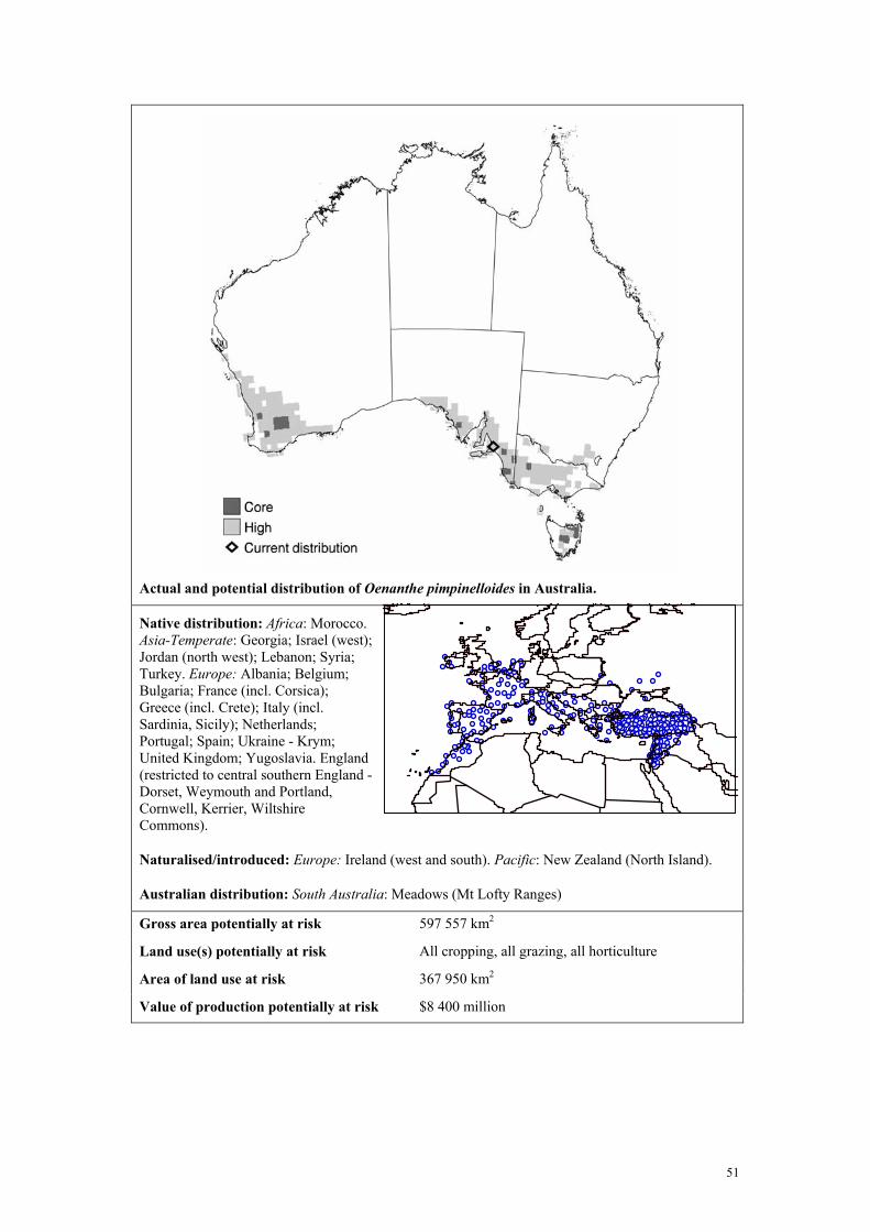
Actual and potential distribution of Oenanthe pimpinelloides in Australia.

Native distribution: Africa: Morocco. Asia-Temperate: Georgia; Israel (west); Jordan (north west); Lebanon; Syria; Turkey. Europe: Albania; Belgium; Bulgaria; France (incl. Corsica); Greece (incl. Crete); Italy (incl. Sardinia, Sicily); Netherlands; Portugal; Spain; Ukraine - Krym; United Kingdom; Yugoslavia. England (restricted to central southern England - Dorset, Weymouth and Portland, Cornwell, Kerrier, Wiltshire Commons).

Naturalised/introduced: Europe: Ireland (west and south). Pacific: New Zealand (North Island).

Australian distribution: South Australia: Meadows (Mt Lofty Ranges)





_p p p

52

Actual and potential distribution of Onopordum tauricum in Australia.

Native distribution: Europe: Bulgaria; Greece (incl. Crete); Romania; Ukraine – Krym. Asia-Temperate: Cyprus; Turkey.

Naturalised/introduced: North America: Arizona, California

Australian distribution: Victoria: Natimuk, Euroa, Violet Town.





53

Actual and potential distribution of Piptochaetium montevidense in Australia.

Native distribution: South America: Argentina; Bolivia; south Brazil; Chile; Paraguay; Peru; Uruguay; Ecuador.


Australian distribution: Victoria: Cherry Lake (Altona).


Land use(s) potentially at risk All cropping, all grazing



54

Actual and potential distribution of Rorippa sylvestris in Australia.

Native distribution: Africa: North Africa. Asia-Temperate: Georgia; Lebanon; Russian Federation (Ciscaucasia); Syria; Turkey. Europe: Albania; Austria; Belarus; Belgium; Bulgaria; Czechoslovakia; Denmark; Estonia; France (incl. Corsica); Germany; Greece; Hungary; Ireland; Italy (incl. Sardinia, Sicily); Latvia; Lithuania; Moldova; Netherlands; Poland; Portugal; Romania; Russian Federation (European part); Spain; Sweden (south); Switzerland; Ukraine (incl. Krym); United Kingdom; Yugoslavia.

Naturalised/introduced: North America/Canada: California, North Carolina, Oregon, Washington, Idaho, Montana, Texas, Alabama, Mississippi, Rochester New York, southern and eastern Canada (Great Lakes, Lake Huron). Asia: Hokkaido, Japan.

Australian distribution: South Australia: Mylor Creek, Zadow’s Landing, Mypolonga; Tasmania: Cradoc, New Norfolk.





55

Appendix D. Feasibility of eradication assessments

Development of a model of eradication cost Since there are no published methods of quantifying the relative feasibility of eradication, we developed a system of quantifying the relative amount of effort required to eradicate a weed based on limited knowledge of its current distribution and biological attributes. The system draws heavily on methods under development to assess feasibility of containment (Virtue 2002) and feasibility of eradication (Panetta and Timmins in prep.). The key difference in our approach was that we calibrated the attributes of a weed against an estimate of the cost involved in an eradication campaign to determine the weightings of each attribute. This was done by a survey of individuals with expertise in weed eradication. Survey respondents were asked to examine each of 15 hypothetical weed profiles and estimate the probability of eradicating the weed for each of 8 broad cost ranges, based only on the attributes described in the profile. The cost ranges represent the maximum total cost over the life of an eradication effort. A detailed costing was not required because the method was designed primarily to assess the relative probability of eradication, not the absolute cost.

The weed profiles were made up of 13 variables that describe the geographic distribution and biological attributes of a weed that are thought to influence the amount of effort involved in eradication. Some factors that affect the feasibility of eradication were not measured in the scoring system. For example, it was assumed that the hypothetical species were not commercially traded and that there was a favourable socio-political environment for an eradication effort, i.e. strong community support, political will and no legal barriers. The variables are listed in Table 1 with the categories used to describe the weeds. The variables are described in detail below:

1. Current distribution

1A. The area currently infested by the weed refers to the current gross infestation area. Gross area is the area over which the weed is distributed while net area is the area to which treatment would be applied. It can be assumed that within the gross area there is a medium density of the weed.

1B. The number of infestations influences the area that must be monitored. A distinct infestation is considered to be an aggregation of plants that is not contiguous with the nearest aggregation of plants (approximate scale: > 100 m to 1000 m depending on the gross area).

1C. The maximum distance between infestations influences control effort through increasing travelling time.

1D. The knowledge of current locations is a measure of the degree of confidence that all infestations are known. It influences the amount of effort required to locate further infestations prior to treatment and the likelihood of detecting all infestations. For a successful eradication, all infestations must be detected. A high level of knowledge at the beginning of an eradication campaign increases the probability of success. However, in order to claim a high level of knowledge, adequate surveillance must have been undertaken.

2. Control effort (access, detection and tolerance)

2A. Ease of access relates to effort required to travel to and within infestation sites for treatment and monitoring activities.

56

2B. Shoot growth refers to the length of time that shoots are visible above-ground and relates to ease of detection.

2C. Appearance also relates to ease of detection in terms of how easy the weed is to distinguish amongst other vegetation in the infestation area. Considerations include height of the plant and other factors that may influence its visibility.

2D. Tolerance to control is a measure of how susceptible or resistant a weed is to chemical or physical control methods. It relates to eradication effort in that more treatments are required to kill more tolerant plants.

3. Persistence (ability to recover and spread)

3A. Time to seeding is the period between germination and the first seed set (or production of vegetative fragments in the case of plants which reproduce vegetatively).

3B. Seedbank longevity is related to the length of the eradication effort in terms of treatment and monitoring.

3C. Number of propagules refers to the number of seeds or vegetative propagules produced per plant per year.

3D. Vegetative regeneration capacity can make an infestation more persistent since vegetative fragments can be difficult to kill and difficult to remove completely.

3E. Propagule dispersion is a measure of the maximum distance propagules are likely to disperse per year. Dispersal distances most likely in the range of 100 to 1000 m may include small animals with a shorter range, movement by stock, some wind blown seed, and water dispersal. Dispersals of 20 to 100m may include wind dispersal where seed has wings and seed moved by ants. Dispersal distances <20m would include seed that falls close to the parent plant, and most vegetative reproduction.

57

Table 1. Categorisation of variables for the draft eradication feasibility index (bold text indicates variables that were found to significantly influence the cost of an eradication as described below)

Variable Categories Code1. Current distribution 1A. Area currently infested by the weed Very large (100 to 3000 ha)

Large (50 – 100 ha) Moderate (10 – 50 ha) Small (1 – 10 ha) Very small (<1 ha)

1 2 3 4 5

1B. Number of infestations Many (>3) Few (2 to 3) One

1 2 3

1C. Maximum distance between infestations Widely scattered (>10 km) Scattered (5 to 10 km) Moderately localised (1 to 5 km) Localised (100 to 1000 m) Zero or <100 m

1 2 3 4 5

1D. Knowledge of current locations Medium (location of most infestations known) High (location of all infestations known)

1 2

2. Control effort (access, detection and tolerance) 2A. Ease of access Low (most sites difficult to access)

Medium (most sites easily accessible) High (all sites easily accessible)

1 2 3

2B. Shoot growth Short (< 4 months) Long (4 to 8 months) Always present (12 months)

1 2 3

2C. Appearance Not distinctive at any stage Distinct in flower Always distinct

1 2 3

2D. Tolerance to control High (difficult to kill with herbicides, repeated applications required in combination with other treatment methods) Medium (several applications of herbicide are required to kill most plants) Low (most plants are killed by a single herbicide application)

1 2 3

3. Persistence (ability to recover and spread) 3A. Time to seeding Short (≤1 year)

Medium (2 year to 3 years) Long (>3 years or never)

1 2 3

3B. Propagule longevity Long (>5 years) Medium (3 to 5 years) Short (<2 years)

1 2 3

3C. Number of propagules High (>2000) Medium high (1000 to 2000) Medium low (50 to 1000) Low (<50)

1 2 3 4

3D. Vegetative regeneration bulbs, corms, rhizomes and/or stem fragments suckers none

1 2 3

3E. Most likely maximum propagule dispersion per year

Most likely to disperse >1 km Most likely to disperse 100 to 1000 m Most likely to disperse 20 to 100 m Most likely to disperse <20 m

1 2 3 4

58

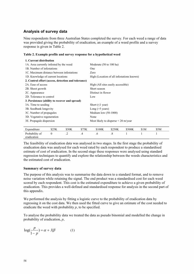
Analysis of survey data Nine respondents from three Australian States completed the survey. For each weed a range of data was provided giving the probability of eradication, an example of a weed profile and a survey response is given in Table 2.

Table 2. Example profile and survey response for a hypothetical weed

1. Current distribution 1A. Area currently infested by the weed Moderate (50 to 100 ha) 1B. Number of infestations One 1C. Maximum distance between infestations Zero 1D. Knowledge of current locations High (Location of all infestations known) 2. Control effort (access, detection and tolerance) 2A. Ease of access High (All sites easily accessible) 2B. Shoot growth Short season 2C. Appearance Distinct in flower 2D. Tolerance to control Low 3. Persistence (ability to recover and spread) 3A. Time to seeding Short (≤1 year) 3B. Seedbank longevity Long (>5 years) 3C. Number of propagules Medium low (50-1000) 3D. Vegetative regeneration None 3E. Propagule dispersion Most likely to disperse < 20 m/year

Expenditure $25K $50K $75K $100K $250K $500K $1M $5M Probability of eradication

0 .2 .4 .6 .8 1 1 1

The feasibility of eradication data was analysed in two stages. In the first stage the probability of eradication data was analysed for each weed rated by each respondent to produce a standardised estimate of cost of eradication. In the second stage these responses were analysed using standard regression techniques to quantify and explore the relationship between the weeds characteristics and the estimated cost of eradication.

Summary of survey data

The purpose of this analysis was to summarise the data down to a standard format, and to remove noise variation while retaining the signal. The end product was a standardised cost for each weed scored by each respondent. This cost is the estimated expenditure to achieve a given probability of eradication. This provides a well-defined and standardised response for analysis in the second part of this appendix.

We performed the analysis by fitting a logistic curve to the probability of eradication data by regressing it on the cost data. We then used the fitted curve to give an estimate of the cost needed to eradicate the weed with probability p, to be specified.

To analyse the probability data we treated the data as pseudo binomial and modelled the change in probability of eradication, p,

βα Xp

p+=

−)

1log( (1)

59

where X is the cost and α and β are parameters to be estimated. We modelled the variation in p as

)1()var( ppp −∝

This is a standard method of analysis (e.g. McCullagh and Nelder 1989). This component of the model specified the weight to be put on the observations.

The model chosen was based on the hypothesis that there is a true underlying probability of eradication that follows the functional form above, and that each respondent gives an unbiased estimate of this, with the variation of the reported responses being proportional to var(p). The data was then used to estimate the values of the parameters. While this assumption cannot be exactly true, in practice the model was being used as a simple summary and interpolation technique.

The model was fitted to the survey responses producing 135 curves, Figure 1 is an example fit.

Figure 1. Plot of observed data versus fitted model for an example weed scored by a survey respondent.

To produce the estimated cost for a given probability p, we rearranged Equation 1 to obtain

βα

ˆˆ)1/log( −−

=ppX

In this analysis we choose to set p=.95, which means X is the estimated cost of a program to eradicate the weed that has a 95% probability of succeeding. The results of the analysis is not driven by this choice, and 95% represents effectively 100% eradication probability without the technical difficulties this choice would introduce.

60

Analysis of significant variables

The output of the analysis above was a cost of eradication. The analysis found that there were 24 cases out of 135 where the algorithm did not converge. This was due in 23 cases to eradication being considered certain for all costs. This response indicates that the respondent felt the 95% eradication cost was less than the lowest available cost on the survey sheet. In these cases a value of $10,000 for the 95% cost was imputed. While more sophisticated techniques could be used to perform this imputation, their effect on the final analysis would be minor and would not warrant the additional overhead in their application. A single weed was estimated as having zero probability of eradication for any costs and this observation was excluded from the analysis.

As the aim of the analysis is to relate the expert assessment of cost with the characteristics of the weeds a multiple regression analysis was considered. Several issues had to be addressed. First the small sample size available meant that the analysis could not consider complicated models with large numbers of parameters. This was achieved by fitting the ordered categorical variables as linear terms in the initial analysis. Once model selection procedures had focused on the key variables the categorical formulation was used to produce the final output. The use of interaction terms was also limited because of the sparseness of the data. Again, interaction terms were considered once initial model selection had occurred. The final issue to consider is the scale of the data. Initial analysis indicated that there was a strong relationship between the variation in the data and the mean. Given this a log transformation of the response was used which greatly improved the analysis. All model results are presented on this scale, with only the final predictions back transformed onto the real scale.

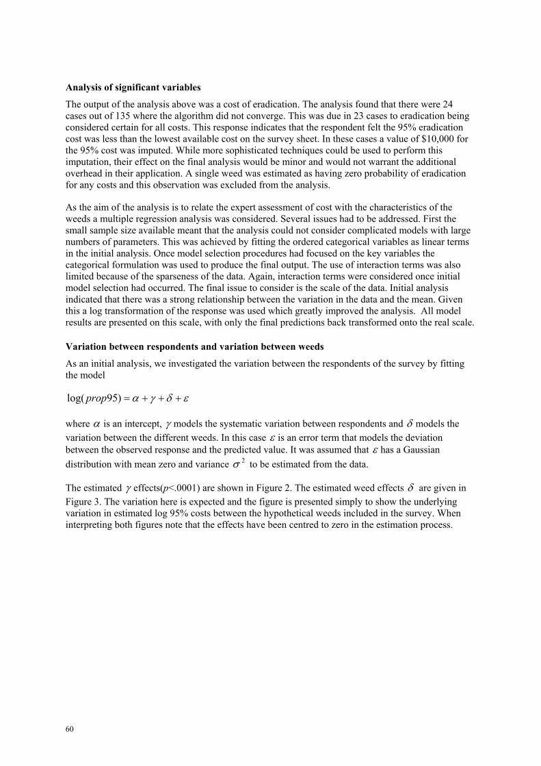
Variation between respondents and variation between weeds

As an initial analysis, we investigated the variation between the respondents of the survey by fitting the model

εδγα +++=)95log( prop

where α is an intercept, γ models the systematic variation between respondents and δ models the variation between the different weeds. In this case ε is an error term that models the deviation between the observed response and the predicted value. It was assumed that ε has a Gaussian distribution with mean zero and variance 2σ to be estimated from the data.

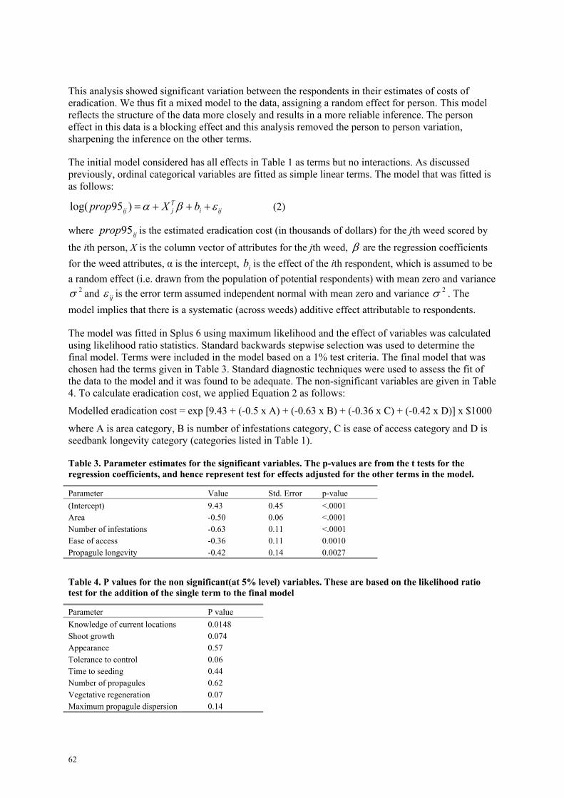
The estimated γ effects(p<.0001) are shown in Figure 2. The estimated weed effects δ are given in Figure 3. The variation here is expected and the figure is presented simply to show the underlying variation in estimated log 95% costs between the hypothetical weeds included in the survey. When interpreting both figures note that the effects have been centred to zero in the estimation process.

61

Figure 2. Plot of estimated PERSON effects, i.e. mean difference between the nine respondents averaged over all weeds.

Figure 3. Plot of estimated SPECIES effects i.e. mean difference between the estimated eradication costs for the 15 hypothetical weeds.

62

This analysis showed significant variation between the respondents in their estimates of costs of eradication. We thus fit a mixed model to the data, assigning a random effect for person. This model reflects the structure of the data more closely and results in a more reliable inference. The person effect in this data is a blocking effect and this analysis removed the person to person variation, sharpening the inference on the other terms.

The initial model considered has all effects in Table 1 as terms but no interactions. As discussed previously, ordinal categorical variables are fitted as simple linear terms. The model that was fitted is as follows:

ijiTjij bXprop εβα +++=)95log( (2)

where ijprop95 is the estimated eradication cost (in thousands of dollars) for the jth weed scored by

the ith person, X is the column vector of attributes for the jth weed, β are the regression coefficients for the weed attributes, α is the intercept, ib is the effect of the ith respondent, which is assumed to be a random effect (i.e. drawn from the population of potential respondents) with mean zero and variance

2σ and ijε is the error term assumed independent normal with mean zero and variance 2σ . The model implies that there is a systematic (across weeds) additive effect attributable to respondents.

The model was fitted in Splus 6 using maximum likelihood and the effect of variables was calculated using likelihood ratio statistics. Standard backwards stepwise selection was used to determine the final model. Terms were included in the model based on a 1% test criteria. The final model that was chosen had the terms given in Table 3. Standard diagnostic techniques were used to assess the fit of the data to the model and it was found to be adequate. The non-significant variables are given in Table 4. To calculate eradication cost, we applied Equation 2 as follows:

Modelled eradication cost = exp [9.43 + (-0.5 x A) + (-0.63 x B) + (-0.36 x C) + (-0.42 x D)] x $1000

where A is area category, B is number of infestations category, C is ease of access category and D is seedbank longevity category (categories listed in Table 1).

Table 3. Parameter estimates for the significant variables. The p-values are from the t tests for the regression coefficients, and hence represent test for effects adjusted for the other terms in the model.

Parameter Value Std. Error p-value (Intercept) 9.43 0.45 <.0001 Area -0.50 0.06 <.0001 Number of infestations -0.63 0.11 <.0001 Ease of access -0.36 0.11 0.0010 Propagule longevity -0.42 0.14 0.0027

Table 4. P values for the non significant(at 5% level) variables. These are based on the likelihood ratio test for the addition of the single term to the final model

Parameter P value Knowledge of current locations 0.0148 Shoot growth 0.074 Appearance 0.57 Tolerance to control 0.06 Time to seeding 0.44 Number of propagules 0.62 Vegetative regeneration 0.07 Maximum propagule dispersion 0.14

63

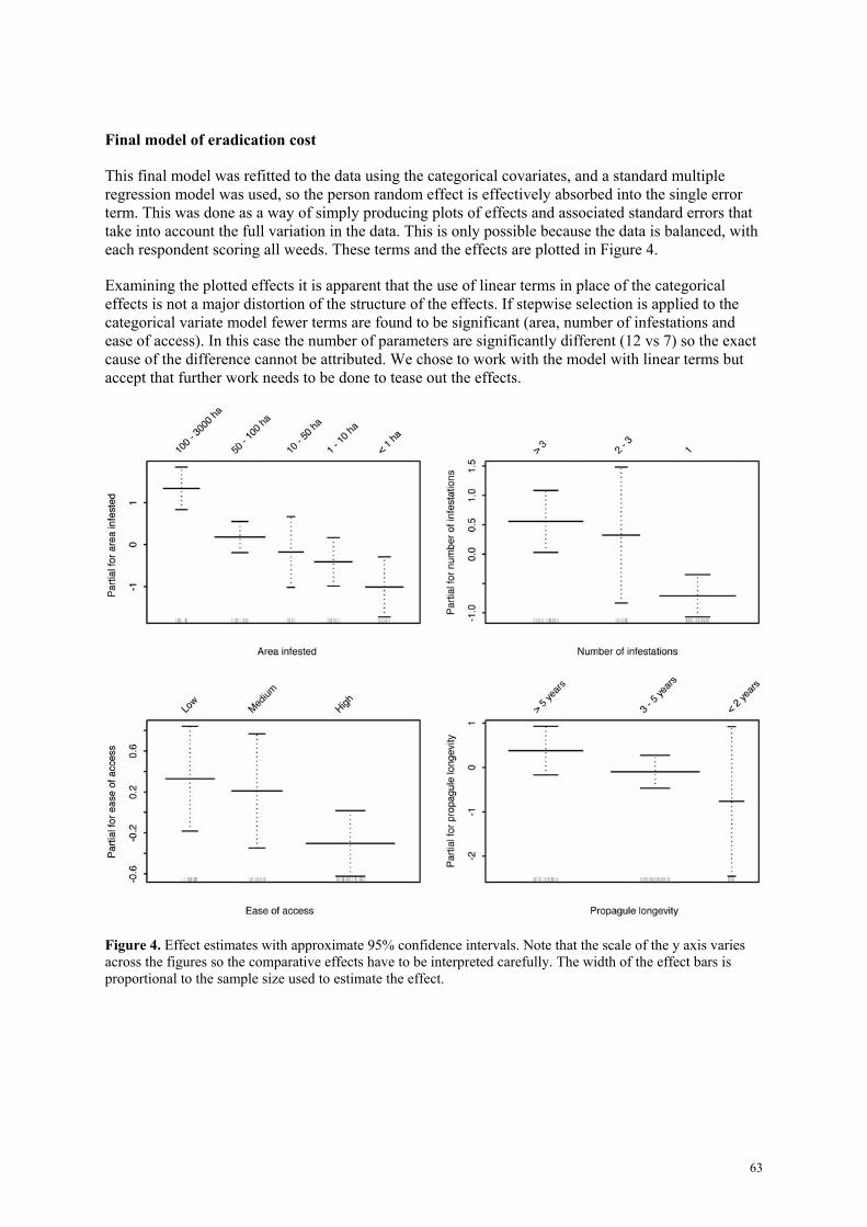
Final model of eradication cost

This final model was refitted to the data using the categorical covariates, and a standard multiple regression model was used, so the person random effect is effectively absorbed into the single error term. This was done as a way of simply producing plots of effects and associated standard errors that take into account the full variation in the data. This is only possible because the data is balanced, with each respondent scoring all weeds. These terms and the effects are plotted in Figure 4.

Examining the plotted effects it is apparent that the use of linear terms in place of the categorical effects is not a major distortion of the structure of the effects. If stepwise selection is applied to the categorical variate model fewer terms are found to be significant (area, number of infestations and ease of access). In this case the number of parameters are significantly different (12 vs 7) so the exact cause of the difference cannot be attributed. We chose to work with the model with linear terms but accept that further work needs to be done to tease out the effects.

Figure 4. Effect estimates with approximate 95% confidence intervals. Note that the scale of the y axis varies across the figures so the comparative effects have to be interpreted carefully. The width of the effect bars is proportional to the sample size used to estimate the effect.

64

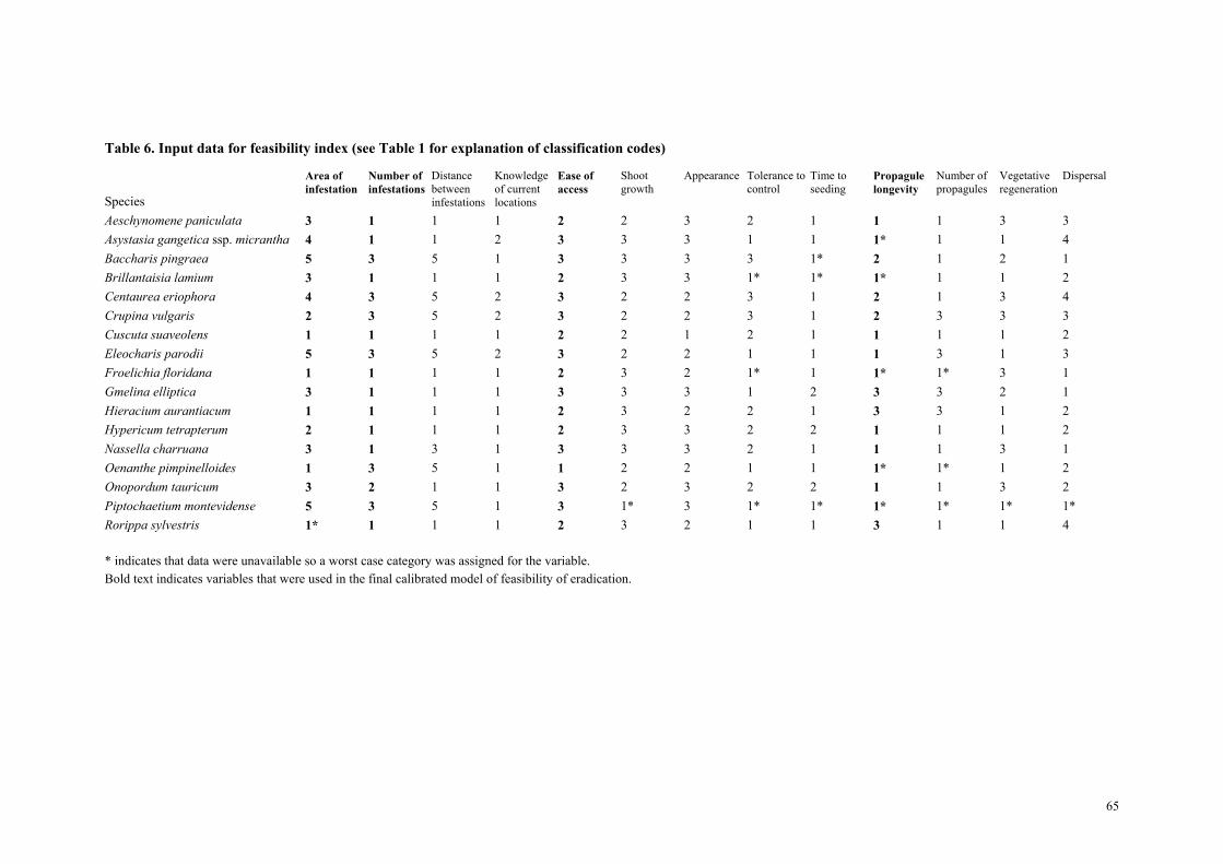
Application of the model to 17 candidate sleeper weeds Input data for all 13 variables in the initial model was obtained for 17 candidate sleeper weeds from the literature and, in the case of geographic distribution, from experts in each State where the species is found. This data is presented in Table 6 with the four parameters used in the final model highlighted in bold text.

Table 5 show the results of the analysis. Note that these costs should be interpreted carefully. First, they are based on estimated eradication probabilities and not actual eradication data. Second, they are based on broad categorization of the weeds attributes. In any actual eradication campaign more detailed estimates would clearly be more reliable and useful in planning. The estimates that are produced are useful for filtering out the candidate weeds, which was the aim of the current process.

Table 5. Relative feasibility of eradication of 17 candidate sleeper weeds

Species Feasibility ranking

Modelled eradication cost

Baccharis pingraea 1 $23,500 Eleocharis parodii 2 $35,100 Piptochaetium montevidense * 3 $35,100 Centaurea eriophora 4 $38,600 Crupina vulgaris 5 $104,000 Gmelina elliptica 6 $146,000 Onopordum tauricum 7 $175,000 Asystasia gangetica ssp. micrantha * 8 $198,300 Nassella charruana 9 $325,300 Aeschynomene paniculata 10 $457,000 Brillantaisia lamium * 11 $457,000 Oenanthe pimpinelloides * 12 $502,000 Hieracium aurantiacum 13 $553,000 Rorippa sylvestris ** 14 $553,000 Hypericum tetrapterum 15 $750,000 Cuscuta suaveolens 16 $1,230,000 Froelichia floridana * 17 $1,230,000 * indicates species for which information on propagule longevity could not be obtained, in these case the longest longevity category was used in the model and the feasibility of eradication could be higher. ** indicates a species for which an estimate of area was unavailable and the largest area category was used, in this case the largest area category was used in the model and the feasibility of eradication could be higher or lower.

References McCullagh, P. and Nelder, J.A. (1989) Generalized linear models, 2nd ed. Chapman and Hall.

Panetta, F.D. and Timmins, S.M. (in preparation) The feasibility of eradication for terrestrial weed incursions.

Virtue, J. (2002) Feasibility of containment - working draft only. Animal and Plant Control Commission Department of Water, Land and Biodiversity Conservation, South Australia.

65

Table 6. Input data for feasibility index (see Table 1 for explanation of classification codes)

Species

Area of infestation

Number of infestations

Distance between infestations

Knowledge of current locations

Ease of access

Shoot growth

Appearance Tolerance to control

Time to seeding

Propagule longevity

Number of propagules

Vegetative regeneration

Dispersal

Aeschynomene paniculata 3 1 1 1 2 2 3 2 1 1 1 3 3 Asystasia gangetica ssp. micrantha 4 1 1 2 3 3 3 1 1 1* 1 1 4 Baccharis pingraea 5 3 5 1 3 3 3 3 1* 2 1 2 1 Brillantaisia lamium 3 1 1 1 2 3 3 1* 1* 1* 1 1 2 Centaurea eriophora 4 3 5 2 3 2 2 3 1 2 1 3 4 Crupina vulgaris 2 3 5 2 3 2 2 3 1 2 3 3 3 Cuscuta suaveolens 1 1 1 1 2 2 1 2 1 1 1 1 2 Eleocharis parodii 5 3 5 2 3 2 2 1 1 1 3 1 3 Froelichia floridana 1 1 1 1 2 3 2 1* 1 1* 1* 3 1 Gmelina elliptica 3 1 1 1 3 3 3 1 2 3 3 2 1 Hieracium aurantiacum 1 1 1 1 2 3 2 2 1 3 3 1 2 Hypericum tetrapterum 2 1 1 1 2 3 3 2 2 1 1 1 2 Nassella charruana 3 1 3 1 3 3 3 2 1 1 1 3 1 Oenanthe pimpinelloides 1 3 5 1 1 2 2 1 1 1* 1* 1 2 Onopordum tauricum 3 2 1 1 3 2 3 2 2 1 1 3 2 Piptochaetium montevidense 5 3 5 1 3 1* 3 1* 1* 1* 1* 1* 1* Rorippa sylvestris 1* 1 1 1 2 3 2 1 1 3 1 1 4 * indicates that data were unavailable so a worst case category was assigned for the variable. Bold text indicates variables that were used in the final calibrated model of feasibility of eradication.

Documents

Appendix A. Short-listing process - Home - Department of