Embed Size (px)
Citation preview


Appendix A1: Work Breakdown Structure
Project Luna Mission WBS
Concept Study
Concept Generation
Trade OffDefine Structure of Satellite
LauncherOrbit
Functional Analysis Tree
Design Option Tree
Configuration Definition
Cost
Weight
Lander/Probe
Payload
4.0
4.2 4.3
4.3.1
4.3.2
4.3.3
4.4
4.5.1
4.5.2
4.5 4.7
risk assassment
4.6 4.8

Design Definition Simulation Report Presentation
5.0 6.0 7.0 8.0

Research
Investigate Location
Investigate Orbit
Investigate Lander/Probe
Investigate PayloadWork
Breakdown Structure
Gantt-chart
Functional Block Diagram
Phase Diagram
Investigate Requirements
1.0
Project Management
2.0 3.0
1.1
1.2
1.3
1.4
2.1
2.2
2.3
2.4
Sustainable Development
1.5
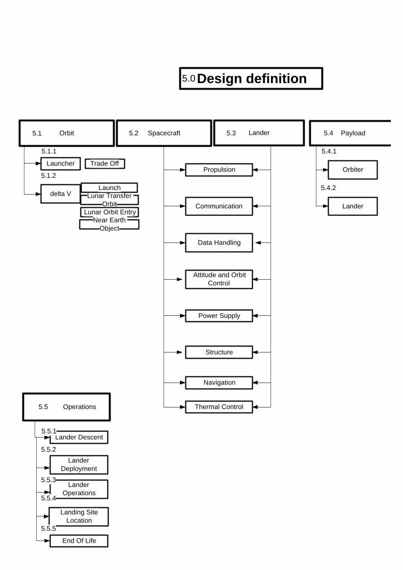
Launcher
delta V
Design definition5.0
5.1.1
5.1.2
Lander Payload5.4
Orbiter
Lander
Lunar TransferOrbit
Lunar Orbit EntryNear Earth
Object
Launch
Trade Off
5.3Spacecraft5.3.2 5.2Orbit5.1
5.4.1
5.4.2
Propulsion
Attitude and OrbitControl
Navigation
Communication
Power Supply
Structure
Thermal Control
Data Handling
Lander Descent
Landing SiteLocation
End Of Life
5.5 Operations
LanderDeployment
LanderOperations
5.5.1
5.5.5
5.5.4
5.5.3
5.5.2

type of fuel
burning time
engine
Propulsion
Attitude and Orbit Control
Navigation
Communication
Power Supply
Structure
Thermal Control
5.2.4
5.2.5
5.2.6
5.2.7 Calibration IMU
Simulation
5.2.1
5.2.3
Thermal Ranges
Single Node Computation
Heating&Cooling
System Components
loads life cycle
moments of inertia
cg computation
dimensionssolar arrays
batteries
attitude determination
attitude control
Data Handling
5.2.8
frequency selection
command distributer
data acquisition
antenna selection
link budget5.2.2
Spacecraft5.2 Lander
Propulsion
Attitude and Orbit Control
Navigation
Communication
Power Supply
Structure
Thermal Control
5.3.2
5.3.4
5.3.5
5.3.6
5.3.7 Calibration IMU
Simulation
5.3
5.3.1
5.3.3
Thermal Ranges
Single Node Computation
Heating&Cooling
System Components
loads life cycle
moments of inertia
cg computation
dimensionssolar arrays
batteries
attitude determination
attitude control
type of fuel
amount of fuel
specific Impuls
Data Handling
5.3.8
frequency selection
command distributer
data acquisition
antenna selection
link budget

Appendix A2: Work Packages
Input Output Who
1.0
1.1 work Work Breakdown Structure C,A,G,W
1.2 work Gantt Chart C,A,G,W
1.3 work Phase Diagram W,G
1.4 work Functional Block Diagram B,V,J,M,P
1.5 future Sustainable development all
2.0
2.1 Detection methods for ice research V,M,W
2.2 Combination configuration C,J
2.3 Possible orbits, possible launchers B,G
2.4 Candidate ice deposits A,P
3.0 Requirements Discovery Tree M,P
4.0
4.1 V,J,M,W
4.2 orbit B
4.3
4.3.1 Functional Analysis Tree P,A,C
4.3.2 Design Option Tree P,A,C
4.3.3 Configuration Definition P,A,C
4.4 concepts cost all
4.5
4.5.1 weight of concepts P,A,C
4.5.2 lander/probe concepts P,A,C
4.6 launcher G
4.7 risk all
4.7 different concepts Final Concepts all
4.8 different concepts Final Concepts all
6.0 Simulation
7.0 Report all
8.0 Presentation all

5.0 Ouput who
5.1 Orbit
5.1.1 Launcher Trade Off G
5.1.2 Delta V :launcher, LTO,Lunar Orbit Entry, NEO B
5.2 Spacecraft
5.2.1 Propulsion B
5.2.2 Communication J
5.2.3 Data Handling J
5.2.4 Attitude and Orbit Control V
5.2.5 Power supply W
5.2.6 Structure M
5.2.7 Navigation G
5.2.8 Thermal Control A
5.3 Lander
5.3.1 Propulsion C
5.3.2 Communication J
5.3.3 Data Handling J
5.3.4 Attitude and Orbit Control V
5.3.5 Power supply W
5.3.6 Structure M
5.3.7 Navigation G
5.3.8 Thermal Control A
5.4 Payload
5.4.1 Orbiter P,C
5.4.2 Lander P,C
5.5 Operations
5.5.1 Lander Descent C
5.5.2 Lander Deployment P,C
5.5.3 Lander Operations P,C
5.5.4 Landing site location P,A
5.5.5 End of life P

Appendix A3: Product Tree The 'MiMiR' Spacecraft consists of a spacecraft bus and a spacecraft payload. The spacecraft payload can be devided in the lander and orbiter instruments. This lander itself also has a bus and instruments on board. All the components of the "Mars Express Re-use"-concept are listed in this Product Tree. The reason this product tree was made is to provide a structured view of the different components of our spacecraft.This helps in designing the components, as to make sure no parts are left out of the design.
Spacecraft (MiMiR)
Spacecraft Bus
Spacecraft Payload
LanderOrbiter
Instruments
Lander BusLander
Instruments
Housing/protection
Solar Panels
Batteries/power distribution
On-board Computer
Wiring
Communications hardware
Thrusters (Main and attitude control)
Lander Interface
Navigation Sensors
Fuel Tanks and lines
Temperature Control Hardware
On-board Computer
Communications Hardware
Batteries/Power Distribution
Wiring
Housing/protection
Thrusters (main and attitude control)
Navigation sensors
Temperature Control Hardware
6 Tunable Diode Lasers
Robotic Sampling System
CCD Camera
Microscopic Imager
Miniature Ground Penetrating Radar
Nanokhod Rover
HRSC
OMEGA
GRS
Neutron Spectrometer
Laser Altimeter
Raman Spectrometer

Appendix A4 : Functional Block Diagram (FBD)
Design Satellite
Problem Definition
Requirements Analysis
Concept Design
Design Definition
Simulation
ValidationSystem
IntegrationSystem Design
Trade OffConcept DefinitionConcept
Generation
1.0
1.1
1.2
1.3
1.4
1.5
1.3.1 1.3.2 1.3.3
1.4.1 1.4.3 1.4.3

Manufacturing Satellite
Systems Testing
Assembly
Systems Manufacture
Parts Manufacture
Testing
2.0
2.1
2.2
2.3
2.2.1
2.2.2
Operate Satellite Disposal Satellite
Lander Deployment
Gather Data
Travel
Launch
Mission preparation
Gather Lander Data
Launch Preparation
Transport to Launch Site
Prepare Mission Plan
Release/Orbit insertion
Launch
Orbit adjustment
Moon OrbitTransfer Orbit
RelayGather DataTest/Calibrate Instruments
Activate Instruments
DeploymentLandingDescentReleaseOrbit
adjustment
RelayGather Data
Test/Calibrate Instruments
Activate Instruments
Travel
De-orbit
3.0
3.1
3.2
3.3
3.4
3.5
3.6
3.1.1 3.1.2
3.2.1
3.2.13.2.1
3.6.1
3.5.1
3.4.1
3.3.1
3.2.2
3.3.2
3.4.2
3.5.2
3.6.2
3.2.3
3.3.3
3.4.3 3.4.4
3.5.3 3.5.4
3.6.3 3.6.4 3.6.5
3.5.5
4.0
4.1

Appendix A5: Requirements Discovery Tree
Mission Requirements
Other Requirements
Determination of location
Quantification of ice
Determination of composition
Cost as low as possible (100-120
M euro wish)
Massdependent of
Launcher
Reliability(tbd)
Life Spanmax. 2 year
x-y position of ice
z position of ice (depth)
Take n number of test
samples of volume/weight
(tbd)
Detection specific
substances A B C (tbd)
Determination of physical
state
Affect as little of the
hydrogen resources as
possible
The mission must be
innovative in some way (*)
Structure must be strong enough to
reach moon
Polar orbit around moon
MiMiR
proof the existance of hydrogen containing substances
must be able to measure till
(x) m depth(tbd)
(*): This can be for example an innovative concept design, an
innovative new system/instrument or even
innovatively combining various systems.


Appendix A6: N2Chart
Payload (Philip+Christ
iaan) orbit altitude
data quantities /
rate
data quantities /
rate
thermal interface & dissipation
mass orbiter payload &
mass lander
Mission Design
(Philip+Christiaan)
exact
trajectory
autonomous?
descent speed
relative propellant
mass & delta V landing
delta V (Bert) exact
trajectorydelta V's
delta V's & fuel weight
engine mass &
dimensions system
Propulsion
(Bert) lunar orbit fuel weight
dimensions
& mass system
Navigation
(Gert) fuel weight
dimensions & mass
system and stabilisation
of lander
Fuel Weight Stabilisation
(Veerle)
does sattelite spin during lunar-
transfer orbit?->no
dimensions & mass system
Communication (Jasper)
dimensions & mass system
Data-handling (Jasper)
dimensions & mass system
Power Supply
(Willem)
available power & batteries
dimensions & mass system
Temperature antennas
Thermal Control
(Annemarie)
!max295kg! (or less if fuel needs
more mass)
everything :-)
!max 1500 m/s!
moments of inertia
thermal interface
Structure (Myrthe)

Appendix A7: Gantt Chart: HARDCOPY INVOEGEN VANUIT MS PROJECT!

Appendix A8: Scoring Functions
0
1
2
3
4
5
6
7
8
9
10
0 20 40 60 80 100 120
Mass [kg]
Sco
re
0
1
2
3
4
5
6
7
8
9
10
0 20 40 60 80 100 120 140
Power [W]
Sco
re
Sustainable Development
0
2
4
6
8
10
Low Avg High
Sco
re
Costs, Risk, Development Time
0
2
4
6
8
10
Low Avg High
Sco
re

Appendix B
B.1 : NON INTRUSIVE PAYLOAD
Neutron spectrometers Gamma ray spectrometers IR spectrometers Microwave spectrometers Miniature Ground Penetrating Radar (Netlander) Radar Altimeter (SSRA, Mars Express) Laser Altimeter (LIDAR, used on Clementine) Raman Spectrometer Optical cameras
B.2 : PAYLOAD IN-SITU Gas analysis and Organic Geochemistry Package Evolved Gas Analyser, elemental molecular composition; COSAC Permittivity Probe (PP) Multi-Purpose Sensor for Surface and Subsurface Science (MUPUS) The Mole Rock Grinder and Corer The Robotic arm Mercury Micro-Rover Tunable Diode Laser Sample Acquisition and Transfer Mechanism Cryogenic Drill (SATM) CMOS Active Pixel Sensor Color Camera (APS) CCD Camera

Appendix B1: Non Intrusive Payload Neutron spectrometers Capabilities Specifications of some neutron spectrometers: Bepi Colombo: The MNS instrument has a mass of 5 kg and consumes 3 W of power. It has a detection range of 0.01 to 5 MeV. Mars Express: The Mars Express neutron spectrometer has a mass of 1.5 kg and consumes 5 W of power. Lunar Prospector: The Lunar Prospector had a neutron spectrometer of 3.9 kg on the orbiter. It detects a characteristic signature for Hydrogen down to a depth of 0.5 meters with a sensitivity of ~50 ppm. Weight: 8.5 pounds (3.9 kilograms) Power: 2.5 Watts Data rate: 49 bits/sec Footprint : 150 km2 Technological maturity The neutron spectrometer has been used on several missions like Lunar Prospector and Clementine. It is a technologically mature instrument and can be used immediately. Issues / Remarks The usual mapping altitude is about 100 km above the surface of the Moon. Gamma ray spectrometers Capabilities Specifications of some gamma ray spectrometers: Lunar Prospector GRS: The Lunar Prospector GRS has a mass of 8.6 kg. It is twice as sensitive as the Apollo GRS but 2 to 5 times less sensitive than a High Resolution GRS. The GRS has a penetrating depth of 10 cm and a nominal orbiting altitude of 150 km. An eccentric orbit is also possible with for instance a periapsis at 10 km. High Resolution GRS: This is an expensive and complex instrument which requires cryogenic cooling to 80 K. It cannot be used on (passive) spin-stabilised spacecraft's. The advantage of the high-purity Germanium sensor is that the lines are very sharp, it has a higher resolution. The count rate is very low, but long integration times permit most elements to be determined. Table B.1 : Characteristics of several gamma-ray spectrometers
Instrument Resolution Energy range Sky coverage TGRS 1.8 keV at 50 keV
2.8 keV at 500 keV 25-8000 keV 2 pi sr
SELENE Ge-detector <3 3 keV at 1.33 MeV KONUS 6 keV at 50 keV
40keV at 500 keV 15-10000 keV 4 pi sr
BATSE 6 keV at 50 keV 5-10000 keV 2.4 pi sr The TGRS thus is more precise but KONUS and BATSE have a bigger range of wavelengths.

Mars Odyssey GRS: This GRS has a mass of 30.5 kg and consumes 32 W of power. Together with the cooler, its dimensions are 46.8 x 53.4 x 60.4 cm. The GRS was developed at the Los Alamos National Laboratory. Bepi Colombo: The MGS weighs 7.5 kg and consumes 5 W of power. Mars Express: The Mars Express GRS has a mass of 2.5 kg and consumes 3 W of power. Technological Maturity The Gamma Ray Spectrometer has been used on several missions to the Moon, Mars etc. It has also been used on satellites which were specially designed for gamma ray spectroscopy (e.g. Compton Gamma Ray Observatory). The technology will also be used in missions like SELENE (Moon) and Bepi-Colombo (Mercury). The technology is thus mature and ready for take-off. Issues / Remarks We will have to pay attention at the ambiguity of the measurements. For instance the gamma-ray lines of Al are at 7.72 MeV, while the ones of Fe are at 7.6 MeV. This can involve inconclusive measurements as the Iron lines can interfere with the Aluminium lines. The H-lines are at 2.223 MeV. We will have to investigate whether these lines interfere with the lines of another element. A second ambiguity can arise as a result of the cosmic background noise. Gamma ray spectroscopy is a space science which deals with a low photon intensity and with a high background level: the GRS is sensitive to gamma rays as well as to other cosmic particles (“Compton photons”and energetic backgrounds). Therefore the GRS consists of a BGO (Bysmuth Germane Crystal) which is sensitive to both the gamma rays and the cosmic particles, and a plastic scintillator which is only sensitive to those background signals and epithermal electrons. If both scintillators give a signal, the GRS detected no gamma ray photon, but a background signal or epi-thermal electrons. If only the BGO scintillator gives a signal, the GRS detected gamma photons. In that way we can get more reliable data. A third ambiguity in the data can arise if we place the GRS too close to the spacecraft. The GRS is mostly placed on a long boom (approximately 6 to 7 m long) attached to the orbiter. If the GRS would be placed on the orbiter, there would be too much interference from gamma rays generated by the spacecraft systems. The nominal mapping altitude of the GRS varies from 100 to 150 kilometres (based upon the Lunar Prospector GRS), but the spacecraft can also be placed in a lower orbit, as the resolution increases then. The accuracy of the measurements increases with the square root of the integration time of the instrument, so a high orbit (low velocity) is desired. On the other hand a high resolution is desired too, so a compromise is necessary. Another option is to increase the mission time of the satellite by a few years (e.g. an elongation of 3 more years). The longer the mission lasts, the more passes have been made over a certain region, the more statistically correct the data will be. This has to do with the low signal to noise ratio as was mentioned earlier. So the longer the GRS measures, the more accurate and reliable the scientific data is. The Lunar Prospector GRS for instance has an integration time of about 30 seconds, but the data can be accumulated as the spacecraft orbits the Moon and passes a certain region frequently.

IR spectrometers Capabilities The IR spectrometer can detect water or water ice. The three different energies which H2O absorbs are the ones which correspond with 3500 cm-1 (2.8 µm), 1650 cm-1 (6.06 µm) and 600 to 300 cm-1 (16.6 – 33.3 µm). The presence of an OH-molecule is indicated at the frequencies between 3200 (3.125 µm) and 3400 cm-1 (2.94 µm). The IR spectroscope will need a range which is broad enough to detect the most interesting particles. Specifications of some IR spectrometers: Bepi Colombo: The IMS (NAC/WAC/IMS) has a mass of 6 kg and uses a power of 10 W. It has a range of 0.8 to 2.8 microns. The instrument was meant for mineral topology with a high resolution, but a moderate spectral resolution. The pixel sizes are 1.25 km and 150 km at low and high altitudes. Cooling is also required until a temperature below 120 K (non operating). Rosetta orbiter: The VIRTIS instrument has a mass of 7 kg and uses a power of 2 to 20 W. It’s visual range is from 0.25 to 1 micron. The Infrared range is from 1 to 5 microns. The instrument can detect lines of H2O, CO, methanol and ice. It requires cooling down to 135 K. Mars Express: The OMEGA instrument weighs 29 kg and has a power use of 22 W. Infrared Space Observatory: This satellite had a Short-Wave Spectrometer aboard, which had a range of 2.5 to 45 microns and a resolving power (λ/∆λ) of about 1000 to 2000. The Long-Wave Spectrometer of ISO has a range of 43 to 196.9 microns. It can operate in two modes: the grating mode, with a resolving power of 1000 to 2500 and a Fabry-Pérot mode (high resolution mode) with a resolving power of 20000 to 30000. The resolution of the two modes is thus very different from each other. The field of view of the LWS is 1.65 arcmin. Mars Global Surveyor: The Thermal Emission Spectrometer (TES) has a range of 6 to 50 microns. It’s dimensions are 24 x 35 x 40 cm and the TES has a mass of 14.4 kg. It uses 14.4 W of power. Mars Odyssey: The THEMIS enhances the TES. It has a mass of 11.2 kg and uses 14 W of power. Its dimensions are 54.5 x 37 x 28.6 cm. It can also detect subsurface water, as well as minerals in water. Technological maturity Infrared spectroscopy has been used several times in the past. Just like is the case with gamma ray spectroscopy, there has even been designed a whole satellite for Infrared spectroscopy (Infrared Space Observatory). Other missions to Mars and Mercury contained an Infrared spectroscope too. The Infrared techniques have been developed very well. The only problem we still have is the fact that the lunar poles where the ice is supposed to be situated, are very cold regions which emit or reflect very few infrared rays. Some research will have to be done on that topic. Issues / Remarks Only passive IR spectroscopy is possible from in orbit. There is a probability that IR spectroscopy won't be successful in our mission because the ice deposit regions do not emit much infrared radiation. An option might be the Raman spectrometer which will be described in paragraph 3.1.13. Microwave spectrometers Capabilities The passive microwave radiometry spectrum lays covers the 200 GHz to 1 GHz band which agrees with 0.15 cm to 30 cm wavelength. The microwave spectrometer has been used on the TOPEX/Poseidon mission. It has a mass of 50 kg and uses 25 W of Power. Also the Rosetta spacecraft will have a microwave spectrometer aboard: MIRO, which has a mass of 23 kg and consumes 5 to 57 W of power.

Technological maturity Very little information was found about microwave spectrometry, and where available, it wasn't suitable for our mission. Microwave spectroscopy seems to be very useful in measuring water vapour in the Earths clouds, but probably not for finding water ice deposits on the Lunar Poles, because of the solid state. Issues / Remarks Passive microwave spectroscopy is possible as well as active spectroscopy. Miniature Ground Penetrating Radar (Netlander) N Provider The Miniature Ground Penetrating Radar (MGPR) which will be put on the Netlander will be designed by the CETP in Paris. The PI for this instrument is Dr. J.J. Berthelier1. We have contacted him through e-mail and he has responded positively. Capabilities The modified version of this instrument will be able to detect changes in dielectric constants of the subsurface materials of the Moon, up to a depth of 20m. Using this data, a detailed picture of the Moon geology can be made. Table B.2: Main characterics of modified Netlander MGPR
Characteristic Value Mass 0.460 kg Dimensions Unknown Power 2-3W Time duration of a measurement ~1h30m Depth range Up to 20m Range resolution 1m (0.5m if possible) Free space wavelength 1.5m (200MHz) Technological Maturity Groud Penetrating Radars are a well developed technology for use on earth; Miniature GPRs such as this one haven’t been produced yet, and are still under development. The MGPR as planned on the Netlander (originally part of the Mars Express mission) will be launched by 2003; research on the short-wave version is expected to start in the fall of 2001 and to be completed by the end of 2003. Issues This instrument will only be useful on a lander, or, more specifically, on a rover, but is has some drawbacks: sampling time is quite long, in the order of 1h30m, during which the instrument should not move substantially. This could cause problems due to the limited amount of power available in the eternal shadows of the lunar South Pole. Apart from that, the redesign needed to use this instrument with a smaller wavelength will take approximately 2 years.

Radar Altimeter (SSRA, Mars Express) Provider This instrument will fly on the ESA Mars Express mission. Capabilities Table B.3: Capabilities of the Mars Express SSRA
Characteristic Value Mass 14kg (?) Dimensions Unknown Power 5/60W (operating/max) Time duration of a measurement Instantaneous Max operating height 600km Range resolution 100m Technological Maturity Radar altimetry is a technology which is used extensively in terrestrial applications. It is a mature and well developed technique which has been applied in several space missions. Issues The high weight and power reqs, when compared to the LIDAR on Clementine, show this instrument is not really an option. However, less heavy instruments are available. Laser Altimeter (LIDAR, used on Clementine) Provider This instrument has been used in orbit by the Clementine mission by NASA. The PI was Dr Eugene Shoemaker. Capabilities Table B.4: Capabilities of the LIDAR Laser Altimeter
Characteristic Value Mass 3kg (estimate) Dimensions Unknown Power 2W (estimate) Time duration of a measurement Instantaneous Max operating height 500km Range resolution 40m
Technological Maturity Laser Altimetry has been used in terrestrial applications and on the Clementine mission successfully. Optimisations leading to lower mass and power consumption should be feasible. Raman Spectrometer Provider

Cornell University is developing a Raman spectrometer for the NASA Mars Exploration missions, to be launched in 2003. Capabilities Table B.5: Capabilities of the Mars Explorer Raman Spectrometer
Characteristic Value Mass 0.3 kg (sensor only) Dimensions Unknown Power Unknown Time duration of a measurement <1s Depth range N/a Range resolution N/a
Technological Maturity Raman Spectrometers are commonly available components for non-space applications. This instrument is being developed right now, and should be in use by 2003. Issues Lots of unknowns in the capabilities table! Availability is another unknown. Optical cameras Capabilities The following two systems are being used as a combination, when put on a spacecraft together, their weight totals 12kg. Narrow Angle Camera (BepiColombo) A Narrow Angle Camera (NAC) is instrument which consists of a set of lenses, a CCD array and a small data processor. Its optical system will have an estimated resolution of about 25 urad/px, which gives the following resolutions for different orbits: Table B.6 : Resolutions and datasizes of the BepiColombo NAC
Altitude (km) Resolution (m/px) Full-coverage datasize (GB) 10 4,7 508 25 12 81
100 47 5.1 250 119 0.81
Depending on the requirements, the optical system can be modified to provide a different resolution, The BepiColombo NAC shares several components with the Wide Angle Camera. Wide Angle Camera (BepiColombo) A Wide Angle Camera (WAC) is an instrument which consists of a set of lenses, a CCD array and a small data processor. Its optical system will have an estimated resolution of about 250 urad/px, which gives the following resolutions for different resolutions for different orbits: Table B.7 : Resolution and datasizes for the BepiColombo WAC
Altitude (km) Resolution (m/px) Full-coverage datasize (MB) 10 47 5080

25 119 810 100 470 51 250 1190 8.1
The BepiColombo WAC shares several components with the Narrow Angle Camera. Issues Necessity of these instruments is questionable, since nice maps of the Moon already exist.

Appendix B2: Payload in-situ Gas analysis and Organic Geochemistry Package Provider The gas analysis and organic geochemistry package is an instrument on board the beagle 2. The instrument is based on the MODULUS concept on board the Rosetta Lander. C.T.Pillinger and I.P.Wright from the Open University, Planetary Sciences Research Institute, have worked on the project and have been contacted: [email protected](personal); [email protected] (general). They have not yet responded. Capabilities The mass spectrometer (Mattauch-Herzog geometry) detector end consists of two types of ion collection devices. The first is a focal plane detector, which can simultaneously measure ion beams across a wide mass window. It can detect and measure the amount of carbon dioxide released on burning the samples. Mounted alongside this detector configured to measure ratios of 13C/12C, 15N/14N, 17O/16O, 18O/16O, and possibly 34S/32S, along with an ancillary detector for H2
+ during measurements of D/H ratios. The gas chromatograph is to support analyses of the gas evolved from pyrolytic oven and a combustion oven respectively. Quantification measurements will be done by pressure sensors. Table B.8 : Gas analysis and Organic Geochemistry Package characteristics
Characteristic Value
Mass 3.685 kg Power(average) 7.8 Watt Sample Size By sample handling system Application On Beagle 2 Deployment Inside Lander Analysis time GC 5 min Resolution GC High Analysis time MS 1 hour Resolution MS Low Analysis time isotope ratio up to 10 hours Data Rate 3.9Mbits
Technological Maturity The Gas analysis and Organic geochemistry Package is an instrument used on the Mars Express mission, it is situated on the lander: the Beagle 2. This is a project by ESA. The instrument operates using the principles of Methods of Determining and Understanding Light elements from Unequivocal Stable (MODULUS) isotopic compositions. This technology has been developed for the Rosetta mission (ESA/NASA mission). These missions have not yet reached their goals, so the instrument has not yet proven its real life reliability, though extensive testing has been done. Lander integration The instrument must be mounted inside the lander, where it can be protected from the low temperature (50K) environment in the Moon crater. The samples will be brought to the instrument by the a robotic arm. Issues The primary issue with the Gas analysis and Organic geochemistry Package is that the instrument has been developed for use in Mars atmosphere, while the Moon has none. Therefore some adjustments to the instrument might be necessary. Thermal control inside the Lander should keep the instrument within its working temperature (dependant of mass spectrometer).
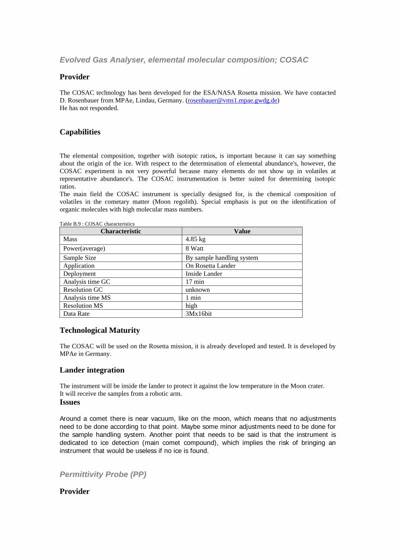
Evolved Gas Analyser, elemental molecular composition; COSAC Provider The COSAC technology has been developed for the ESA/NASA Rosetta mission. We have contacted D. Rosenbauer from MPAe, Lindau, Germany. ([email protected]) He has not responded. Capabilities
The elemental composition, together with isotopic ratios, is important because it can say something about the origin of the ice. With respect to the determination of elemental abundance's, however, the COSAC experiment is not very powerful because many elements do not show up in volatiles at representative abundance's. The COSAC instrumentation is better suited for determining isotopic ratios. The main field the COSAC instrument is specially designed for, is the chemical composition of volatiles in the cometary matter (Moon regolith). Special emphasis is put on the identification of organic molecules with high molecular mass numbers. Table B.9 : COSAC characteristics
Characteristic Value Mass 4.85 kg Power(average) 8 Watt Sample Size By sample handling system Application On Rosetta Lander Deployment Inside Lander Analysis time GC 17 min Resolution GC unknown Analysis time MS 1 min Resolution MS high Data Rate 3Mx16bit
Technological Maturity The COSAC will be used on the Rosetta mission, it is already developed and tested. It is developed by MPAe in Germany. Lander integration The instrument will be inside the lander to protect it against the low temperature in the Moon crater. It will receive the samples from a robotic arm. Issues Around a comet there is near vacuum, like on the moon, which means that no adjustments need to be done according to that point. Maybe some minor adjustments need to be done for the sample handling system. Another point that needs to be said is that the instrument is dedicated to ice detection (main comet compound), which implies the risk of bringing an instrument that would be useless if no ice is found. Permittivity Probe (PP) Provider

The permittivity probe is being used on the Rosetta mission as a part of SESAME. It is developed by DLR, Germany and contact has been made to H. Laakso, FMI Helsinki, [email protected], who is primary investigator of the SESAME project. He has not responded. Capabilities Through Permittivity measurement of the landing site a conclusion can be made about the existence of ice at the Moon surface. Table B.10: Permittivity Probe characteristics
Characteristic Value Mass (total) 0,35 kg Power(average) 0,1 W Application On Rosetta Lander Deployment In Lander feet Data Rate (total) unknown
Technological Maturity The instrument is developed for the Rosetta mission. Lander integration The instrument will be located in the lander feet, in order to make contact with the Moon surface. In the studied documentation no limit for minimum operational temperature could be found. Issues We don't know if the instrument can operate at a temperature of 50 K. So maybe thermal control in the feet is needed. Multi-Purpose Sensor for Surface and Subsurface Science (MUPUS) Provider The MUPUS team exists of the following institutes: Institut für Planetologie, Westfälische Wilhelms-Universität Münster, Germany Space Research Centre, Polish Academy of Sciences, Warsaw, Poland Institut für Weltraumforschung, Österreichische Akademie der Wissenschaften, Graz, Austria DLR Institut für Weltraumsensorik & Planetenerkundung, Berlin, Germany Division of Geological and Planetary Sciences, California Institute of Technology, Pasadena, USA Institute of Geophysics, Warsaw University, Warsaw, Poland We have contacted A. J. Ball, of the Open University, England, [email protected] Capabilities
PEN-temperature (TP)
The PEN-TP experiment aims to measure the vertical temperature
distribution as it evolves with time. (Moon summer-winter differences
could be measured, given the time.)

PEN-thermal conductivity (THC)
The thermal conductivity is one of the most critical parameters of the
comet nucleus energy balance. The thermal conductivity of porous near-
surface material is a strong function of its texture, which is strongly
connected to density, porosity, and the absence or abundance of
volatiles such as water ice or organic that might glue dust particles
together. It may be very small (10-5 –Wm
-1 K
-1 ) in a dry,
organic-free dust mantle or (less probably) fresh porous ice. It
may, however, be as high as about 0.5 Wm-1 K
-1 in a sintered,
well-annealed ice layer or a dust mantle glued by organic compounds.
A combined but independent measurement of the temperature profile and
thermal conductivity measurements would allow us to determine the heat
flow into the interior, which is the source for all features of
activity and alteration of the comet nucleus. The close relation between
texture characteristics (e.g., porosity, density, hardness and the
size of bonds between dust or ice aggregates) on the one hand and the
thermal conductivity on the other offers a further possibility for a
combined interpretation of corresponding experiment data.
PEN-penetrometer (M)
A penetrometer at the lower tip of the sub-surface probe is foreseen
to measure the mechanical strength of the near-surface layers.
Combination of the results with the thermal conductivity data and the
density measurement will further restrict the nature of the material near
the surface. A clear detection of layering is possible. Furthermore,
the shape of the measured insertion force profile usually gives
information about pore sizes and the strength of bonds.
Compton Backscatter Densitometer (CBD)
Determination of the bulk density of the comet's surface layers is of
great importance. The local value can be compared with the bulk density
of the whole nucleus, thus helping to characterise the surface
material. The value obtained by the CBD can also be compared with
that found less directly using knowledge of composition (from other
RoLand experiments) and porosity (from thermal and mechanical data
gathered by PEN). Density is also a key parameter for analysis of
acoustic /
seismic, thermal and mechanical data. For example, a more reliable
value for porosity could be obtained by combining the density with
compositional information.
The densitometer will need no deployment other than contact with the
cometary surface. Beryllium windows in the underside of the RoLand foot
are necessary for the source and detector apertures. Table B.11: MUPUS characteristics
Characteristic Value Mass (total) 0.897 kg Power(average) 1.05 Watt Application On Rosetta Lander Deployment on lander, with own arm Analysis time PEN-TP 10 s every 10 min Analysis time PEN-THC 2 hours Analysis time PEN-M one-off measurement Analysis time CBD 1 hour Analysis time TM 10 s Data Rate (total) <9 kbits/meas 4096 bits

Technological Maturity The instruments have been developed for the Rosetta mission, some minor adjustments might be necessary. Lander integration The PEN will be mounted on the lander and will be placed on the Moon surface by an arm. The CBD will be employed in the lander feet and the TM will be mounted on top of the lander. Issues The form of the PEN tip must be determined for optimal data acquisition of the Moon material. Also application at the low temperature must be tested. The Mole Provider The Mole is being used on the Mars Express and on the Bepi Colombo missions. So it is a fully developed technique. Capabilities Sample acquisition from up to a depth of 2m (for the Moon this will be approximately 5m, due to a regolith density of 1700 kg/m3). The Mole will also conduct in-situ measurements like soil temperature at various depths on two locations and assessment of mechanical properties of the subsurface. The mole works for soil or rock pebbles, not for solid rock. Moon regolith will be a good material. The Mole will be retrieved by pulling the cable back. The maximum extraction force is 30N.

Table B.12: Mole characteristics
Characteristic Value Mass (total) <1.8 kg Power(average) 3-6 Watthour Sample Size unknown Application On Beagle2 Deployment on robotic arm Data Rate (total) unknown
Technological Maturity The Mole has been fully developed for the application on the Beagle 2 and future application on the Bepi Colombo mission. A possibility of putting thermal conductivity sensors on the Mole (needing a little heating facility) needs to be investigated and tested. Lander integration On the Beagle 2 the Mole is one of the packages that the Robotic arm can pick and work with. When not in use the Mole will be on the lander and otherwise it will be on the Robotic arm. On the Bepi Colombo the Mole is integrated in the Lander and no Robotic arm is needed. Rock Grinder and Corer Provider It is developed by ESA in combination with the Mole. Same information as for the Mole is applicable for the Grinder. Capabilities The Rock Grinder and Corer will grind rock surface for investigation of the ground area by other instruments, such as the X-ray and Mossbauer spectrometer and the Microscope. It will also sample material from the rocks within the reach of the Robotic arm. The drill is capable of retrieving a sample with a core of 2mm and a length of 1cm; this will be equivalent to approximately 60mg of sample. The typical sample size collected by the drill will allow detection of carbon at sub-parts-per-billion level. Table B.13 : Rock Grinder and Corer characteristics
Characteristic Value Mass (together with Mole) 1.8 kg Power(average) (together with Mole) 3-6 Watt Hour Sample Size 1cm x 2mm, 60 mg Deployment On Robotic arm Application On Beagle 2
Technological Maturity The same as for the Mole is applicable for the Grinder. Lander integration The Grinder is mounted on the Lander when not being used; otherwise it is attached to the Robotic arm. Issues An obscuring weathering rind on rocks like on Mars is not happening on the Moon therefore the Grinder does not give an great extra value to the retrieved rock samples. The material of Moon rock can be examined from the outside as well.

The Robotic arm Provider See the Mole and the Grinder. Capabilities The reach of the Robotic arm is 0.75m. The maximum weight the Robotic arm can handle will be approximately 1.5kg. Table B.14 : Robotic Arm characteristics
Characteristic Value Mass (together with Mole) 3.17 kg Power(average) (together with Mole) 5 Watt Hour Deployment On Lander Application On Beagle 2
Technological Maturity See Mole and Grinder. Lander integration The Robotic arm will be mounted on the Lander. Issues The Robotic arm should be able to work at a temperature of 50K Mercury Micro-Rover Provider A micro-rover configuration called ‘Nanaokhod’ was first developed at the Max-Planck-Institut für Chemie in Mainz and further improved in co-operation with an industrial contractor. We tried to contact Mr. Brückner on the following address [email protected] but no reply was received. Capabilities A micro-rover for a Mercury lander would have a total mass of 2.5 kg and could accommodate payload of about 500 g consisting of an alpha X-ray spectrometer. A camera for navigation a close-up imager, and, if the mass of the chassis can be further reduced a Mossbauer spectrometer are possible additional payload elements. The tether allows a traverse of about 100 m, and is pulled out from a spool located on the rover. Table B.15 : Micro-Rover Characteristics
Characteristics Value Mass Total: 2500g
Rover 1600g Payload 500g Lander based equipment 400g
Dimensions 20 cm x 16 cm x 6 cm (stowed position) Supply voltage 28 V Power during operation 2 W average, max.3 W Minimum time of operation 1 h per sample (accumulated) Minimum life time 1 month Telemetry 19.2 kb/s from rover to lander

Sensitivity to contamination None Maximum tolerable shock 250 g x 25 ms
Technological Maturity This type of rover has not yet been used in a mission but will be used in the BepiColombo mission planned for 2009. Lander Integration The micro-rover restraints are incorporated into the Mercury lander, and their release simultaneously activated along with the opening of the access panel located in the sidewall. The micro-rover is free to exit the lander but remains connected to the Mercury lander by an umbilical cable. Issues The main issue is that the rover only can carry a payload of 500g and must be able to work at a temperature of 50K. Tunable Diode Laser Provider Tunable diode lasers have been supplied for multiple Mars missions by the Jet Propulsion Laboratory with aid from the Lunar and Planetary Laboratory of the University of Arizona (Dr. Bill Boynton and Dr. Ralph Lorenz) and the University of California at Los Angeles. There was a correspondence with Dr. Lorenz. ([email protected]) Capabilities Tunable diode laser sensors can accurately determine the concentration of particular gaseous substances within gaseous samples, such as atmospheres. Water and carbon dioxide are the most commonly measured materials using TDL sensors in space missions. Additionally, concentrations of isotopic variations of these substances can be determined by examining results at energies corresponding to the different isotopes. A single diode laser can distinguish hydrogen from deuterium and well as the carbon isotopes from each other, as each isotope has absorption lines near, but not overlapping, those of the other isotopes. Additionally if the ice is vaporised in an absorption cell it is possible to measure the quantification of substances in the sample. The tunable diode laser capabilities listed in the following table are based on the smallest, most recent Mars TDL sensor, the Mars Microprobes of Deep Space 2. This sensor was specifically designed for small size as well as water detection. Water has absorption peaks near 2.7 and 1.5 mm for all isotopes. Table B.16 : TDL Characteristics
Characteristics Value Mass 11 grams Volume 5.2 cubic centimeters Power 1.5 Watts peak
Computing On-board chip Operational Temperature Range > -120°C Sample Size 100 milligrams

Analysis Time Minutes Precision 1 % Detection Range (Concentration) 7.5 x 10¹⁰ to 5 x 10¹⁵ molecules/ cm3 Technological Maturity The TDL technology is well developed and flight-ready. A small, single-analysis TDL is being used for water detection on the Mars 98 mission as part of the Deep Space 2 Mars Microprobes. A large, multiple-use TDL is being used for water and other volatile detection as part of the Thermal Evolved Gas Analyzer on the Mars 98 Mars Polar Lander. Lander Integration In order to allow the laser to make a long path-length through a gaseous sample, two methods may be used: • Sample Return: A sample may be returned from down-hole to the surface and deposited in a sample chamber where it is volatilised by a heat source. The SATM drill has this capability. Sample return may lead to sublimation of some of the water ice, reducing concentration measurements. • On-Drill Analysis: A sample could be analysed nearly in-situ by building a sample chamber of the interior of the drill shaft. The laser and detector could be incorporated into the top of the drill, where they may be thermally controlled. A mirror would be required inside the drill at the bottom of the sample chamber in order to reflect the light back to the detector. This would also require a heat source at the drill tip in order to volatilise the sample and a means of sending power to it. These modifications may require increases in the drill diameter and power. Issues The primary issue remaining is the method of integrating the TDL with the rover in order to maintain temperature and sample integrity and permitting analysis. Although the operational temperature range must be > -120°C, the TDL can be used. The TDL must be integrated inside the lander where the temperature is controlled.
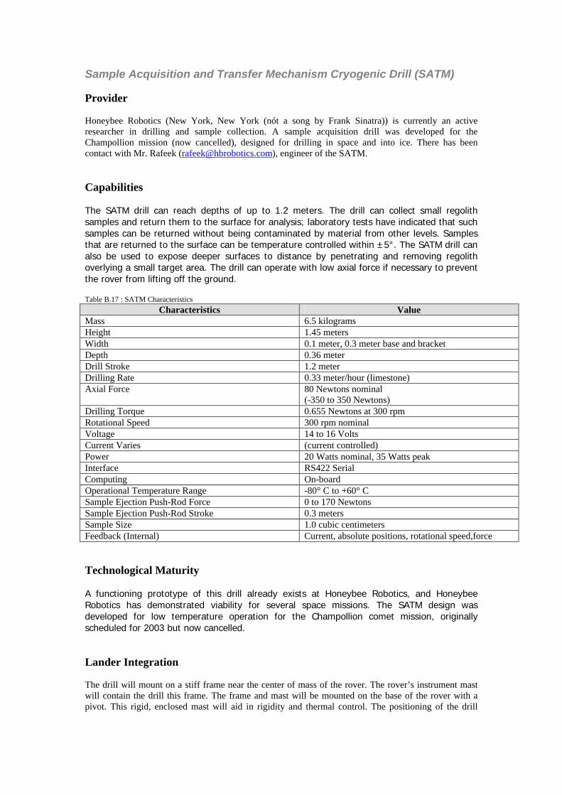
Sample Acquisition and Transfer Mechanism Cryogenic Drill (SATM) Provider Honeybee Robotics (New York, New York (nót a song by Frank Sinatra)) is currently an active researcher in drilling and sample collection. A sample acquisition drill was developed for the Champollion mission (now cancelled), designed for drilling in space and into ice. There has been contact with Mr. Rafeek ([email protected]), engineer of the SATM. Capabilities The SATM drill can reach depths of up to 1.2 meters. The drill can collect small regolith samples and return them to the surface for analysis; laboratory tests have indicated that such samples can be returned without being contaminated by material from other levels. Samples that are returned to the surface can be temperature controlled within ±5°. The SATM drill can also be used to expose deeper surfaces to distance by penetrating and removing regolith overlying a small target area. The drill can operate with low axial force if necessary to prevent the rover from lifting off the ground. Table B.17 : SATM Characteristics
Characteristics Value Mass 6.5 kilograms Height 1.45 meters Width 0.1 meter, 0.3 meter base and bracket Depth 0.36 meter Drill Stroke 1.2 meter Drilling Rate 0.33 meter/hour (limestone) Axial Force 80 Newtons nominal
(-350 to 350 Newtons) Drilling Torque 0.655 Newtons at 300 rpm Rotational Speed 300 rpm nominal Voltage 14 to 16 Volts Current Varies (current controlled) Power 20 Watts nominal, 35 Watts peak Interface RS422 Serial Computing On-board Operational Temperature Range -80° C to +60° C Sample Ejection Push-Rod Force 0 to 170 Newtons Sample Ejection Push-Rod Stroke 0.3 meters Sample Size 1.0 cubic centimeters Feedback (Internal) Current, absolute positions, rotational speed,force Technological Maturity A functioning prototype of this drill already exists at Honeybee Robotics, and Honeybee Robotics has demonstrated viability for several space missions. The SATM design was developed for low temperature operation for the Champollion comet mission, originally scheduled for 2003 but now cancelled. Lander Integration The drill will mount on a stiff frame near the center of mass of the rover. The rover’s instrument mast will contain the drill this frame. The frame and mast will be mounted on the base of the rover with a pivot. This rigid, enclosed mast will aid in rigidity and thermal control. The positioning of the drill

close to the center of mass allows the rover to withstand greater drilling torque and axial forces without slippage or lifting off the ground. To prevent reduction of ground clearance for driving, the bottom of the drill bit is mounted flush with the floor of the rover’s body. The drill is 1.45 meters tall with the drill screw fully retracted, which places the top of the mast at nearly 2.0 meters above the ground. The drill and instrument mast stow horizontally for launch, flight, and landing. This reduces the effects of launch forces on the mast, as well as the size of the envelope required to contain the rover. A spring-loaded device activates the one-time deployment of the instrument/communications mast. The deployment mechanism includes an axle pin with dual redundancy to reduce the risk of deployment failure. Once deployed, the mast latches into place. As the drill is actuated, it cannot operate in the low temperatures of permanent dark. Heating elements will be required on the motors for operation in these regions. Issues The primary issue remaining with the SATM drill is drill depth. It is desired to be able to drill at least 1.0 meter below the surface, and the current drill allowing for ground clearance only allows for drilling 0.75 meters down. This may be adequate to detect water, but extending the drill or changing the mounting to allow for deployment closer to the ground must be considered. Although the operational temperature range of the SATM is between -80° C to +60° C the drill can be used on the cold spots. Only the motors have to be heated. CMOS Active Pixel Sensor Color Camera (APS) Provider The APS has been developed by the JPL MicroDevices laboratory, led by Dr. Bedabrata Pain. Contact has been made with JPL but no response yet. ([email protected]) Capabilities The APS cameras are versatile in their capabilities and models. In all cases, high-resolution images are produced and stored in 8- or 10-bit monochrome or 8-bit color. High dynamic range and signal-to-noise ratios provide high performance while using low power and being small. Typical characteristics are shown below. Table B.18 : CMOS APS Imager Characteristics Characteristic Value
NASA prototype Value PB-300
Mass 0.125 kg Unavailable, similar Size 7.5 by 2.5 by 3 cm Unavailable, similar Power 5 mW (per 100K pixels)
3.3 V 300 mW (maximum) 5 V 6 mA
Resolution (Pixel Size) < 20 µm 7.9 µm Image Size 512 horizontal
512 vertical 640 horizontal 487 vertical
Noise 5 e- RMS 15 e- RMS > 20 db SNR
Efficiency 25-50 % Unavailable Frame Rate 30 frames/sec 0-39 frames/sec Dynamic Range > 75 db 75 db
The characteristics listed here compare a commercially available color camera (from Photobit) and the NASA current prototype.
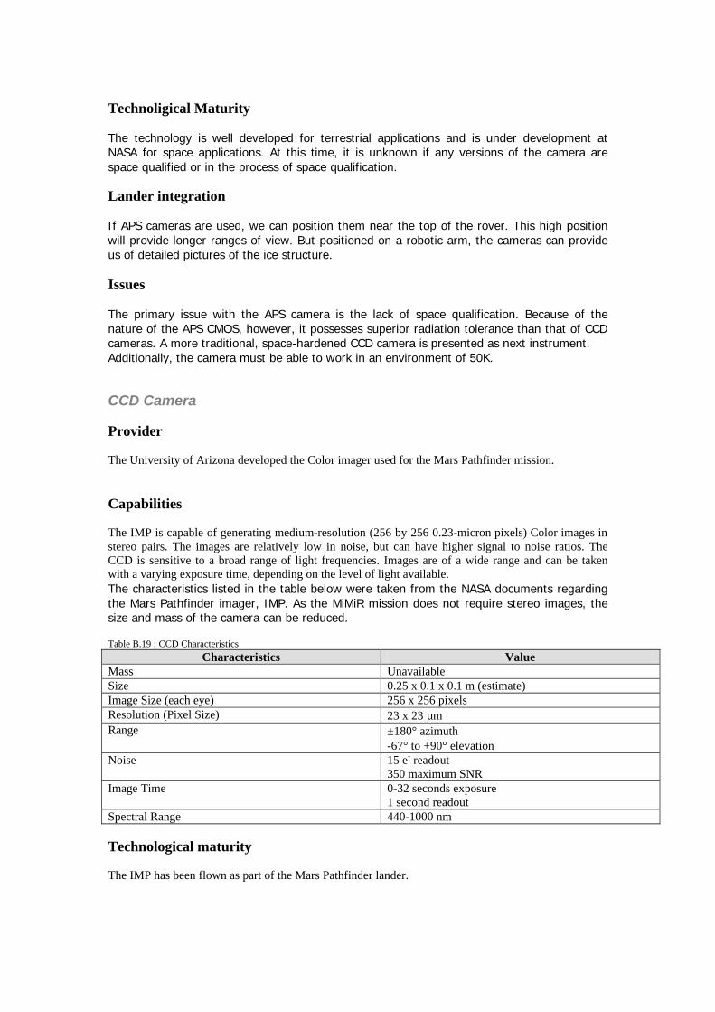
Technoligical Maturity The technology is well developed for terrestrial applications and is under development at NASA for space applications. At this time, it is unknown if any versions of the camera are space qualified or in the process of space qualification. Lander integration If APS cameras are used, we can position them near the top of the rover. This high position will provide longer ranges of view. But positioned on a robotic arm, the cameras can provide us of detailed pictures of the ice structure. Issues The primary issue with the APS camera is the lack of space qualification. Because of the nature of the APS CMOS, however, it possesses superior radiation tolerance than that of CCD cameras. A more traditional, space-hardened CCD camera is presented as next instrument. Additionally, the camera must be able to work in an environment of 50K. CCD Camera Provider The University of Arizona developed the Color imager used for the Mars Pathfinder mission. Capabilities The IMP is capable of generating medium-resolution (256 by 256 0.23-micron pixels) Color images in stereo pairs. The images are relatively low in noise, but can have higher signal to noise ratios. The CCD is sensitive to a broad range of light frequencies. Images are of a wide range and can be taken with a varying exposure time, depending on the level of light available. The characteristics listed in the table below were taken from the NASA documents regarding the Mars Pathfinder imager, IMP. As the MiMiR mission does not require stereo images, the size and mass of the camera can be reduced. Table B.19 : CCD Characteristics
Characteristics Value Mass Unavailable Size 0.25 x 0.1 x 0.1 m (estimate) Image Size (each eye) 256 x 256 pixels Resolution (Pixel Size) 23 x 23 µm Range ±180° azimuth
-67° to +90° elevation Noise 15 e- readout
350 maximum SNR Image Time 0-32 seconds exposure
1 second readout Spectral Range 440-1000 nm Technological maturity The IMP has been flown as part of the Mars Pathfinder lander.

Lander integration A pair of single CCD cameras of the IMP type would be integrated on the same manner of the APS camera. Issues Although the APS camera has better performance, the CCD camera is more reliable because it is space qualified and already been used in other missions. Additionally, the camera has to work in an environment of 50K.

Appendix C
Table C1: Launchers Launcher Available launch costs
(M$) orbit (km)
payload (kg)
success rate (%)
Soyuz Available 13,48 – 28,08 LEO:200 200 200 250
7100 6700 6250 6550
98 (1025/1060)
Soyuz-Ikar Operational 42,30 LEO:400 400 1400
3600 3850 2500
100 (6/6)
Soyuz-Fregat Operational 37,02 LEO:500 1000 1500 200/10000
5300 4900 4500 3100
100 (4/4)
Start-1 Operational 4,16 – 8,32 100 (3/3)
SS-18K Operational 25,12 – 50,24 LEO:200/200 200/200 200/1000 200/1000
4400 4100 3700 3500
100 (1/1)
Tsyklon
Operational 11,89 – 17,83 LEO:200 200 600
3600 2820 2900
98 (240/245)
Zenit Operational 42,68 – 54,87 LEO:200 GTO:200/3600
13740 3820
81,2 (26/32)
J-1 Operational 33,53 – 40,47 LEO:250 GTO
1000 200
100 (1/1)
M-5 Operational 41,62 LEO:250 1800 100 (2/2)
Athena I Available 19,62 LEO:370 700 66,5 (2/3)
Athena II Operational 29,72 LEO:180 185 185
1450 1914 1976
66,67 (2/3)
Titan 2 Operational 38,16 LEO:185 3175 95,24 (20/20)
Taurus Available 20,70 LEO:400 1250 100 (5/5)
CZ 4 Available 32,43 LEO:200 GTO:200/35800
4200 1500
100 (5/5)
PSLV Operational 23,78 – 29,72 LEO:400 GTO
3000 450
80 (4/5)
VLS Available 17,57 0

Appendix D
Soyuz-Fregat

Tsyklon Taurus

CZ-4 / LM-4

Appendix E
Appendix E1: Mass breakdown Table E.1 : Orbiter payload mass breakdown
Instrument name Weight (kg)HRSC 21,2OMEGA 29Neutron spec. 5Laser alt. 6,5GRS:MRS 7,5
Total 69,2 Table E.2 : Orbiter elements mass breakdown
Element Weight (kg)Bus dry mass 500Payload 69,2Propellant 348Lander 130
Total 1047,2 Table E.3 : Lander payload mass breakdown
Instrument name Weight (kg)TDL (6x) 0,3Raman Spectrometer 1,75CCD 0,83Microscopic Imager 0,075Lamp 0,1Nanokhod Rover 1,45GPR 0,46RSS/N 1,1Permittivity Probe 0,35
TOTAL 6,415

Table E.4 : Lander subsystems mass breakdown
Subsystem Part Weight (kg)Navigation CCD descent camera 0,5
INS 4,5radar alt 0,6
Thermal control RHU (75 x) 3Power batteries & wiring 5Attitude Determination & Control thrusters 1,2
propellant 1Data handling & Communications antennas (2x) 0,4
compu 2,5Propulsion engine & tanks 10
propellant 65Structure 15Payload 6,4Subtotal 115,1
10% system margin 11,51
TOTAL 126,61

Appendix E2: Views of the lander
figure E.1 : Inside view of lander
Figure E.2: Isometric views of lander

Appendix E3: Qbasic simulation of landing phase SCREEN 12: CLS : WINDOW (-2000, -200)-(0, 1300) mumaan = 4903.5: th = 0: t = 0: msc = 130: f = 0: h = 0: qq = 1: tb2 = 0: rmaan = 1737.4 vy = 1.688: vx = 0: x = -1757.4: y = 0 FOR q = 0 TO 8 * ATN(1) STEP .001 PSET (1737.4 * COS(q), 1737.4 * SIN(q)) NEXT q 90 amoon = mumaan / (x ^ 2 + y ^ 2) t = t + .1 LOCATE 20, 60: PRINT "t="; t LOCATE 21, 60: PRINT "f="; f LOCATE 22, 60: PRINT "altitude:"; alt LOCATE 23, 60: PRINT "vtotal="; vt LOCATE 24, 60: PRINT "msc="; msc ax = -(x / SQR(x ^ 2 + y ^ 2)) * amoon ay = -(y / SQR(x ^ 2 + y ^ 2)) * amoon vx = vx + .1 * ax + .1 * ax2 vy = vy + .1 * ay + .1 * ay2 vt = SQR(vx ^ 2 + vy ^ 2) h = SQR(x ^ 2 + y ^ 2) alt = h - 1737.4 IF t > 0 AND t < 37.6 THEN f = 1 IF t > 37.6 THEN qq = 0: eb = 1 IF qq = 1 THEN fx2 = -SGN(vx) * SQR((vx / vt) ^ 2) * 2200 IF qq = 1 THEN fy2 = -SGN(vy) * SQR((vy / vt) ^ 2) * 2200 IF qq = 1 THEN ax2 = fx2 / (msc * 1000) ELSE ax2 = 0 IF qq = 1 THEN ay2 = fy2 / (msc * 1000) ELSE ay2 = 0 IF qq = 1 THEN msc = msc - .083 IF eb = 1 AND alt < 4.25 AND vt > .02 THEN f = 2 IF eb = 1 AND alt < 4.25 AND vt < .02 THEN f = 0 IF eb = 1 AND alt < .05 AND vt > .008 THEN f = 2 IF eb = 1 AND alt < .05 AND vt < .008 THEN f = 0 IF msc < 60 THEN f = 0 IF alt < .025 THEN f = 0 IF f = 2 THEN fx2 = -SGN(vx) * SQR((vx / vt) ^ 2) * 2200 IF f = 2 THEN fy2 = -SGN(vy) * SQR((vy / vt) ^ 2) * 2200 IF f = 2 THEN ax2 = fx2 / (msc * 1000) ELSE IF f = 0 AND eb = 1 THEN ax2 = 0 IF f = 2 THEN ay2 = fy2 / (msc * 1000) ELSE IF f = 0 AND eb = 1 THEN ay2 = 0 IF f = 2 THEN msc = msc - .083 IF f = 2 THEN tb2 = tb2 + .1 x = x + .1 * vx y = y + .1 * vy IF alt < 0 AND vt > .012 THEN LOCATE 22, 10: PRINT "CRASH": GOTO 1000 IF alt < 0 AND vt < .012 THEN LOCATE 22, 10: PRINT "LANDED": GOTO 1000 PSET (x, y) IF t > 400 THEN PSET (-900 + (t - 400) * 8, f * 100 + 700) GOTO 90 1000 PRINT "vt ="; vt PRINT "vx="; vx PRINT "vy="; vy PRINT "msc="; msc PRINT "2nd burn time"; tb2

Appendix F
Appendix F1: Euler buckling !!! Maple uitprinten en dan invoegen!!!

Appendix F2: shear flow of the lander !!!! Maple worksheet uitprinten en dan invoegen!!!!(naam landerconstr)

Appendix F3: limit loads of adapter 937 at separation plane

Appendix F4: Mass moments of inertia


Appendix F5: drawings of the Mars Express.


1. Payload interface area available on top floor (top floor sizes 1700 mm x 1500 mm)

Payload interface area available on top floor (top floor sizes 1700 mm x 1500 mm)


Appendix G
Appendix G1: Navigation instruments specification Appendix G2: Kalman Filter Appendix G3: Results navigation simulation Appendix G4: Matlab Source Code: A close-loop control-navigation sensor calibration problem

Appendix G1: Navigation instruments specification Inertial Measurement Unit
Figure G.1: Inertial Measurement Unit Features • 3 axis angular rate and velocity measurement unit using GG1320 RLG and QFLEX (ISO2000)
accelerometers • Space radiation hardened electronics > 100 Krads, latch up immune, SEU tolerant • Powered from +28 Vdc • RS422 serial output (optional 1553 interface) • Expansion capability for specialised user interface • Temperature compensated output over -30°C to +70°C • < 15 second turn on • Built in test • S2418mall (7.8"d x 5.2"h) • lightweight (9.0 lb) • power consumption < 34 W Table G.1 : Typical sensor performance
Gyro Accelerometer Range Bias (1σ) ARW(1σ) Scale factor (1σ) IA Alignement (1σ)
± 375 deg/sec < 0.05 deg/hr < 0.01 deg/DHr < 5 ppm < 25 arc-sec
± 25g < 100 µg < 175 ppm < 70 µrad

CCD descent camera Table G.2: Descent camera data sheet
Instrument Descent camera for a Lander on Moon Objective Range Resolution Field of View Pointing Mass Dimensions Preferred location Power Telemetry Temperature Range Operational altitude Sun aspect angle Other requirement
Imaging of the surface at several wavelengths during the descent 300 nm to 1000 nm 1 mrad/px 58° x 58° direction: slightly downwards camera head: 0.5 kg camera head: 10 x 5 x 5 cm underside of lander 8 W peak (during filter motor drive), 3 W (during imaging) 2 kb/s continuous buffered by memory operation: < 0 C Stand-by: -80 to +40 C 20 km – 100 m no direct pointing to Sun around 0.2 Gb memory for data storage
Radar Altimeter
Figure G.2 : Radar Altimeter
This is a small light weight (0.4 kg) RA. The current design is capable of sensing from a range of 4.5 km, but with a height tolerance of approximately ± 200 m. The suppliers have stated that the operational height can be extended to 40 km, but with a mass (0.6 kg) and measurement tolerance (± 2.0 km) penalty. However, any initial tolerance shall improve with reduction in lander approach height. The altimeter is a stand-alone unit, with a standard RS232 interface. It shall be switched on at a pre-determined time and continually generate a radar beam (4.3 GHz) over a cone angle of 70°.
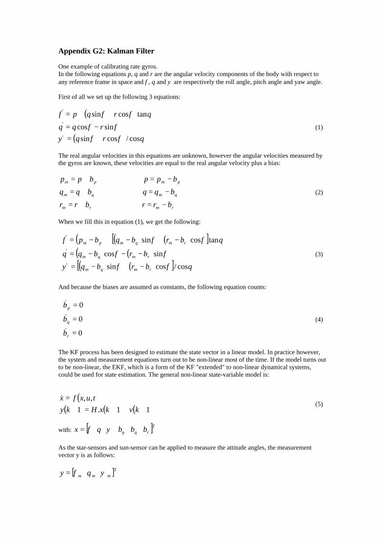
Appendix G2: Kalman Filter One example of calibrating rate gyros. In the following equations p, q and r are the angular velocity components of the body with respect to any reference frame in space and φ, θ and ψ are respectively the roll angle, pitch angle and yaw angle. First of all we set up the following 3 equations:
( )
( ) θφφψφφθ
θφφφ
cos/cossin
sincos
tancossin
rq
rq
rqp
+=−=
++=
&
&
&
(1)
The real angular velocities in this equations are unknown, however the angular velocities measured by the gyros are known, these velocities are equal to the real angular velocity plus a bias:
rmrm
qmqm
pmpm
brrbrr
bqqbqq
bppbpp
−=⇒+=
−=⇒+=
−=⇒+=
(2)
When we fill this in equation (1), we get the following:
( ) ( ) ( )[ ]( ) ( )( ) ( )[ ]
−+−=
−−−=
−+−+−=
θφφψ
φφθ
θφφφ
cos/cossin
sincos
tancossin
rmqm
rmqm
rmqmpm
brbq
brbq
brbqbp
&
&
&
(3)
And because the biases are assumed as constants, the following equation counts:
=
=
=
0
0
0
r
q
p
b
b
b
&
&
&
(4)
The KF process has been designed to estimate the state vector in a linear model. In practice however, the system and measurement equations turn out to be non-linear most of the time. If the model turns out to be non-linear, the EKF, which is a form of the KF "extended" to non-linear dynamical systems, could be used for state estimation. The general non-linear state-variable model is:
( )( ) ( ) ( )11.1
,,
+++=+=
kvkxHky
tuxfx& (5)
with: [ ]Trq bbbx pψθφ=
As the star-sensors and sun-sensor can be applied to measure the attitude angles, the measurement vector y is as follows:
[ ]Tmmmy ψθφ =

The recursion process for the EKF is described below:
( ) ( ) ( )( ) ( )
( )( )kkxx
tA
TT
xtuxf
A
e
QkkPkkP
dttuxfkkxkkx
,ˆ
.
,,
with
...,.,1
,,,ˆ,1ˆ
=
∆
∂∂
=
=Φ
ΓΓ+ΦΦ=+
+=+ ∫
( ) ( ) ( )( )( ) ( ){ }
=
++=
+++=+−
000100
000010
000001
H
1.1 with
.,1...,111
kvkvER
RHkkpHHkkpkKT
TT
( ) ( ) ( ) ( ) ( ){ }( ) ( )[ ] ( ) ( )[ ] ( ) ( )1..1.1.,1..11,1
,1ˆ.1.1,1ˆ1,1ˆ
++++−++−=++
+−++++=++
kKRkKHkKIkkPHkKIkkP
kkxHkykKkkxkkxTT
With: x: state vector, dimension n G: input noise matrix y: measurement vector, dimension m R: covariance matrix of process noise H observation matrix calculated at time tk+1 v: measurement system noise, dimension p x̂ (k+1,k): one stage ahead prediction states x̂ (k+1,k+1): measurement update states P(k+1,k): covariance matrix of one stage ahead prediction error P(k+1,k+1): covariance matrix of state estimation error φ: state transition matrix from time tk to time tk+1 Q: covariance matrix of process noise A: linearized system matrix K: Kalman gain Γ: input distribution matrix ∆t: sample time interval
( ) ( ){ } jiT RjvivE ,δ=

Appendix G3: Results navigation simulation Figure G3.1: (Estimated) Roll angle against time Figure G3.2: (Estimated) Pitch angle against time Figure G3.3: (Estimated) Yaw angle against time
--- real trajectory … estimated trajectory
0 100 200 300 400 500 600-0.05
0
0.05
0.1
0.15
0.2
0 100 200 300 400 500 600-0.05
0
0.05
0.1
0.15
0.2
0 100 200 300 400 500 600-0.05
0
0.05
0.1
0.15
0.2

Figure G3.4: Estimated x axis rate gyro bias against time
Figure G3.5: Estimated y axis rate gyro bias against time
Figure G3.6: Estimated z axis rate gyro bias against time
0 100 200 300 400 500 600-0.01
0
0.01
0.02
0.03
0.04
0.05
0 100 200 300 400 500 600-0.01
0
0.01
0.02
0.03
0.04
0.05
0.06
0.07
0 100 200 300 400 500 600-0.005
0
0.005
0.01
0.015
0.02
0.025
0.03
0.035
0.04
0.045

Figure G3.7: x axis gyro bias estimation error against time
Figure G3.8: y axis gyro bias estimation error against time
Figure G3.9: z axis gyro bias estimation error against time
--- axis gyro bias estimation error … standard deviation of the estimation error
100 150 200 250 300 350 400 450 500 550 600-0.5
0
0.5
1
1.5
2
2.5
3
3.5x 10
-5
100 150 200 250 300 350 400 450 500 550 600-0.5
0
0.5
1
1.5
2
2.5
3
3.5x 10
-5
100 150 200 250 300 350 400 450 500 550 600-0.5
0
0.5
1
1.5
2
2.5
3
3.5x 10
-5

Appendix G4: Matlab Source Code: A close-loop control-navigation sensor calibration problem
% A close-loop control-filtering-identification problem % for adaptive spacecraft attitude control % The system state equation is non-linear and observation equation is linear clear;clf; global wvm I=[2500 0 0 0 2300 0 0 0 3000]; Iw=[5 0 0 0 5 0 0 0 5]; wv=[0.001 .001 .001]'; wvb=[0.000014 -0.000014 0.000014]'*pi/180; wvm=wv+wvb; wwv=[0 0 0]'; angles= [0.1 0.1 0.1]'; %.1 .1 .1]'; estangles=angles+0.1; Td=[1e-3 1e-3 1e-3]'; dt=1; N=600; kp=57; kd=500; std=0.001*pi/180; noise=std*randn(3,N); hv=I*wv; hwv=Iw*(wv+wwv); Ts=dt; x_k_1k_1=[estangles' 1e-5 1e-5 1e-5]'; % x(0|0)=E{x_0} P_k_1k_1=diag([1 1 1 1 1 1]); % P(0|0)=P(0) V_ww=diag([0 0 0 (0.000001*pi/180)^2 (0.000001*pi/180)^2 (0.000001*pi/180)^2]); % Covariance matrix system noise V_vv=diag([std*std std*std std*std]); % Covariance matrix measurement noise ti=0; tf=Ts; n=length(x_k_1k_1); % n: state dimension H=[1 0 0 0 0 0 0 1 0 0 0 0 0 0 1 0 0 0]; for i=1:N %Tgv=3*omega0^2/2*[sin(2*angles(1))*cos(angles(2))^2*(I(3,3)-I(2,2)) -sin(2*angles(2))*cos(angles(1))*(I(1,1)-I(3,3)) -sin(2*angles(2))*sin(angles(1))*(I(2,2)-I(1,1))]'; anglesm=angles+noise(:,i); wvm=wv+wvb; A=[1 sin(angles(1))*tan(angles(2)) cos(angles(1))*tan(angles(2)) 0 cos(angles(1)) -sin(angles(1)) 0 sin(angles(1))/cos(angles(2)) cos(angles(1))/cos(angles(2))];

% Extended Kalman Filter (EKF) %============================== % Prediction %------------ x_cor(:,i)=x_k_1k_1; stdx_cor(:,i)=sqrt(diag(P_k_1k_1)); [t,x]=ode45('func1',[ti,tf],x_k_1k_1); % Predicted states based on % former estimates x_kk_1=x(length(t),:)'; % x(k|k-1) (prediction) [Phi,Gamma]=func3(x_k_1k_1,t,n,Ts); % Phi(k,k-1), Gamma(k,k-1) P_kk_1=Phi*P_k_1k_1*Phi'+Gamma*V_ww*Gamma'; % P(k|k-1) (prediction) stdx_pred(:,i)=sqrt(diag(P_kk_1)); % Correction %------------ Ve=(H*P_kk_1*H'+V_vv); % Pz(k|k-1) (prediction) L=P_kk_1*H'*inv(Ve); % K(k) x_kk=x_kk_1+L*(anglesm-H*x_kk_1); % x(k|k) (correction) P_kk=(eye(n)-L*H)*P_kk_1*(eye(n)-L*H)'+L*V_vv*L'; % P(k|k) (correction) %============================= dhwv=(kp*x_kk(1:3)+kd*(wvm-x_kk(4:6))); wvv(i,:)=wv'; wwvv(i,:)=wwv'; dhwvv(i,:)=dhwv'; anglesv(i,:)=angles'; angles=angles+(A*wv)*dt; hv=hv+(Td-dhwv-cross(wv,hv+hwv))*dt; hwv=hwv+(dhwv)*dt; wv=inv(I)*hv; wwv=inv(Iw)*hwv-wv; % Next step x_k_1k_1=x_kk; P_k_1k_1=P_kk; ti=tf; tf=tf+Ts; end

Function 1 function derivx = func1(t,x); global wvm A=[1 sin(x(1))*tan(x(2)) cos(x(1,1))*tan(x(2)) 0 cos(x(1)) -sin(x(1)) 0 sin(x(1))/cos(x(2)) cos(x(1))/cos(x(2))]; derivx(1:3)=A*(wvm-x(4:6)); derivx(4:6)=0; derivx = derivx'; Function 2 function ypred = func2(x); ypred(1:3) = x(1:3); ypred = ypred'; Function 3 function [Phi,Gamma] = func3(x,t,n,Ts) d = 0.001; unit = eye(n); for j = 1:n dx(j)=x(j)*d; x_p = x + unit(:,j)*dx(j); fpl(:,j) = feval('func1',t,x_p); x_m = x - unit(:,j)*dx(j); fmin(:,j) = feval('func1',t,x_m); F(:,j)=(1/(2*dx(j)))*(fpl(:,j)-fmin(:,j)); end G=[1 sin(x(1))*tan(x(2)) cos(x(1))*tan(x(2)) 0 0 0 0 cos(x(1)) -sin(x(1)) 0 0 0 0 sin(x(1))/cos(x(2)) cos(x(1))/cos(x(2)) 0 0 0 0 0 0 1 0 0 0 0 0 0 1 0 0 0 0 0 0 1]; [Phi,Gamma]=c2d(F,G,Ts); Function 4 function H = func4(x,n) d=0.0001; unit=eye(n); for j = 1:n dx(j)=x(j)*d; x_ph = x'+ unit(:,j)*dx(j); zp(:,j)= feval('func2',x_ph'); x_mh = x' - unit(:,j)*dx(j); zm(:,j)= feval('func2',x_mh'); H(:,j) = (1/(2*dx(j)))*(zp(:,j)-zm(:,j)); end

Appendix H
Appendix H1: Simulation programme of the AOCS of the MiMiR Orbiter A simulation programme has been written in order to proove that the AOCS system works. It is also possible to derive, out of the plots, how many times the reaction wheels have to be off-loaded. The simulation is written with the computer programme MATLAB. A linearized theory is assumed and the controllers are coupled. The input variables are: h0: momentum bias of flywheels at the beginning w0: turn rate of orbit reference axis (pitch) I1, I2, I3: principal moments of inertia Td0: disturbance torque estimation thetalim: maximum deviation from nominal attitude With these constants the conrol gains can be calculated, which is described in general in the following: Calculation of control gains Kd and Kp with the basic linear control theory:
standard diagram for single-loop servo system
In this report a so-called PD (Proportion and Differentiation) controller is applied to stabilize the orbiter. The close-loop transfer function is:
θ+θ= &dPd KKT
Calculation of KP:
( )
( )sKKsI
1
sKKsI
11
sI
1
)s(T)s(
dP2
dP2
2
d
++=
++=
θ
The output θ(s) is then:

( )sKKsI
)s(T)s(
dp2
d
++=θ
For worst cases Td is a constant. The Laplace transform of Td is:
The final value theorem can be written as:
P
0d
0st K
T)s)s((lim))t((lim =⋅θ=θ
→∞→
Therefore the proportional gain KP is calculated as:
∞→θ
=
t
0dP )t(lim
TK (1)
The calculation of differentiation gain Kd can be summarized as:
sKKsI
1)s(T
)s(
dP2
d ++=
θ
Characteristic equation: I s2 + Kds + KP = 0 The standard characteristic equation is:
0s2s 2nn
2 =ω+ςω+ If we compare the standard characteristic equation with the one above, we have the natural frequency ωn.
I
K Pn =ω
I
K
I
K
22
2
707.022
:ratiodampingtheassume
dP =⋅⋅
⇓
==ςς
Pd KI2K ⋅⋅= (2)
Formula (1) and (2) have been used in the simulation programme to calculate the control gains. Furthermore is x1 the deviation vector at the beginning and Td(1), Td(2) and Td(3) are disturbance torques. The gravity gradient torque (3D) is calculated with the following equation:
( )( )( )
−φθ−−φθ−−θφ
µ=
xy
zx
yz2
30
gv
IIsin2sin
IIcos2sin
IIcos2sin
R2
3T (**)
In this formula µ = V2R0 = GM (G is the universal gravitational constant, M is the mass of the Moon, µ is the product of the gravitational constant and the mass of the Moon, V is the orbiting velocity and R0
s
T)s(T 0d
d =

is the distance from the satellite to the center of the Moon). The orbital angular velocity is
300
0 RRV µ
==ω .
Substitute this formula in (**):
( )( )( )
−φθ−−φθ−−θφ
ω=
xy
zx
yz2
20
gv
IIsin2sin
IIcos2sin
IIcos2sin
2
3T
This formula is used in the simulation programme. Kinematic equations:
φφ−φφ=φ
cossin0
sincos0
001
A
θθ
θ−θ=θ
cos0sin
010
sin0cos
A
χχ−χχ
=χ
100
0cossin
0sincos
A
θφ
θφ
φ−φθφθφ
=
coscos
cossin
0
sincos0
tancostansin1
A*
ω−−
ωωω
=
χθφ
χθφ
0
0
AAAAA 0*
z
y
x*
&
&
&
This is the final kinematic equation as used in the simulation programme. The vector x is defined as:
[ ]Tzyxzyx hhhx χθφωωω=
For the coupled controllers the following formula is used:
x0d_zp_z
d_yp_y
z0d_xp_x
h)kk()3(Tc
)kk()2(Tc
h)kk()1(Tc
ω+χ⋅+χ⋅−=
θ⋅+θ⋅−=
ω−φ⋅+φ⋅−=
&
&
&
The last term of the first and last equation stated above, is due to the coupling of the controllers. Furthermore the vector Hω has been defined as:
[ ]Tzyx hhhH =ω
This is the angular momentum vector of the reaction wheels.
+
ωωω
⋅×
ωωω
−++=
ωωω
ωHITTT
z
y
x
z
y
xTcgv
Td
z
y
x
&
&
&

[ ]T
ccczyx )3(T)2(T)1(Tx χθφωωω= &&&&&&&
x& is known, as well as x, so the new vector x can be calculated by means of integration:
dtxxx ⋅+= & The resulting vector can be plotted now, which has been done for the three situations: 1. launch, full tanks 2. solar array deployed, full tanks 3. solar array and lander deployed, tanks empty The simulation programme: % Simulation of the AOCS (reaction wheels) in case of % launch and full tanks, % solar array deployed and full tanks and % the solar array and lander deployed with tanks empty % simulation: with coupled controllers % constants: Td0, thetalim, I, w0 clear all; close all; clc; h0=0; %momentum bias of flywheels at the beginning w0=0.05*pi/180; %turn rate of orbit reference axis (pitch) I1=[393.1807 0 0 %launch, full tanks 0 664.8227 0 0 0 691.2049]; I2=[509.8058 0 0 %solar array deployed, full tanks 0 669.0731 0 0 0 953.9716]; I3=[613.4643 0 0 %solar array and lander deployed, tanks empty 0 591.0231 0 0 0 875.9216]; Td0=5e-5; %disturbance torque (worst case) thetalim=0.05*pi/180; %maximum allowable deviation from nominal attitude
(based on lander ejection requirement) %control gains kx_p1=Td0/thetalim; kx_d1=sqrt(2*I1(1,1)*kx_p1); ky_p1=Td0/thetalim; ky_d1=sqrt(2*I1(2,2)*ky_p1); kz_p1=Td0/thetalim; kz_d1=sqrt(2*I1(3,3)*kz_p1); kx_p2=Td0/thetalim; kx_d2=sqrt(2*I2(1,1)*kx_p2); ky_p2=Td0/thetalim; ky_d2=sqrt(2*I2(2,2)*ky_p2); kz_p2=Td0/thetalim; kz_d2=sqrt(2*I2(3,3)*kz_p2); kx_p3=Td0/thetalim; kx_d3=sqrt(2*I3(1,1)*kx_p3); ky_p3=Td0/thetalim; ky_d3=sqrt(2*I3(2,2)*ky_p3); kz_p3=Td0/thetalim; kz_d3=sqrt(2*I3(3,3)*kz_p3); dt=20; tf=200000;

N=tf/dt; x1=[0 0 0 5*pi/180 5*pi/180 5*pi/180 0 0 0]'; %deviation at the beginning for i=1:N; %disturbance torques (worst case) Td(1)=5e-5; Td(2)=5e-5; Td(3)=-5e-5; %gravity gradient torque Tgv1=3*w0^2/2*[sin(2*x1(4))*cos(x1(5))^2*(I1(3,3)-I1(2,2)) -sin(2*x1(5))*cos(x1(4))*(I1(1,1)-I1(3,3)) -sin(2*x1(5))*sin(x1(4))*(I1(2,2)-I1(1,1))]'; Aphi1=[1 0 0 0 cos(x1(4)) sin(x1(4)) 0 -sin(x1(4)) cos(x1(4))]; Atheta1=[cos(x1(5)) 0 -sin(x1(5)) 0 1 0 sin(x1(5)) 0 cos(x1(5))]; Apsi1=[cos(x1(6)) sin(x1(6)) 0 -sin(x1(6)) cos(x1(6)) 0 0 0 1]; A1=[1 sin(x1(4))*tan(x1(5)) cos(x1(4))*tan(x1(5)) 0 cos(x1(4)) -sin(x1(4)) 0 sin(x1(4))/cos(x1(5)) cos(x1(4))/cos(x1(5))]; dx1(4:6)=A1*x1(1:3)-A1*Aphi1*Atheta1*Apsi1*[0 -w0 0]'; %kinematic equation Tc1(1)=-(kx_p1*x1(4)+kx_d1*dx1(4))-w0*x1(9); %coupled controllers Tc1(2)=-(ky_p1*x1(5)+ky_d1*dx1(5)); Tc1(3)=-(kz_p1*x1(6)+kz_d1*dx1(6))+w0*x1(7); hw1=[x1(7) x1(8) x1(9)]'; dx1(1:3)=inv(I1)*(Td'+Tgv1+Tc1'-cross(x1(1:3),(I1*x1(1:3)+hw1))); dx1(7)=Tc1(1); dx1(8)=Tc1(2); dx1(9)=Tc1(3); x1=x1+dx1'*dt; xv1(i,:)=x1'; end x2=[0 0 0 5*pi/180 5*pi/180 5*pi/180 0 0 0]'; %deviation at the beginning for i=1:N; %gravity gradient torque Tgv2=3*w0^2/2*[sin(2*x2(4))*cos(x2(5))^2*(I2(3,3)-I2(2,2)) -sin(2*x2(5))*cos(x2(4))*(I2(1,1)-I2(3,3)) -sin(2*x2(5))*sin(x2(4))*(I2(2,2)-I2(1,1))]'; Aphi2=[1 0 0 0 cos(x2(4)) sin(x2(4)) 0 -sin(x2(4)) cos(x2(4))];
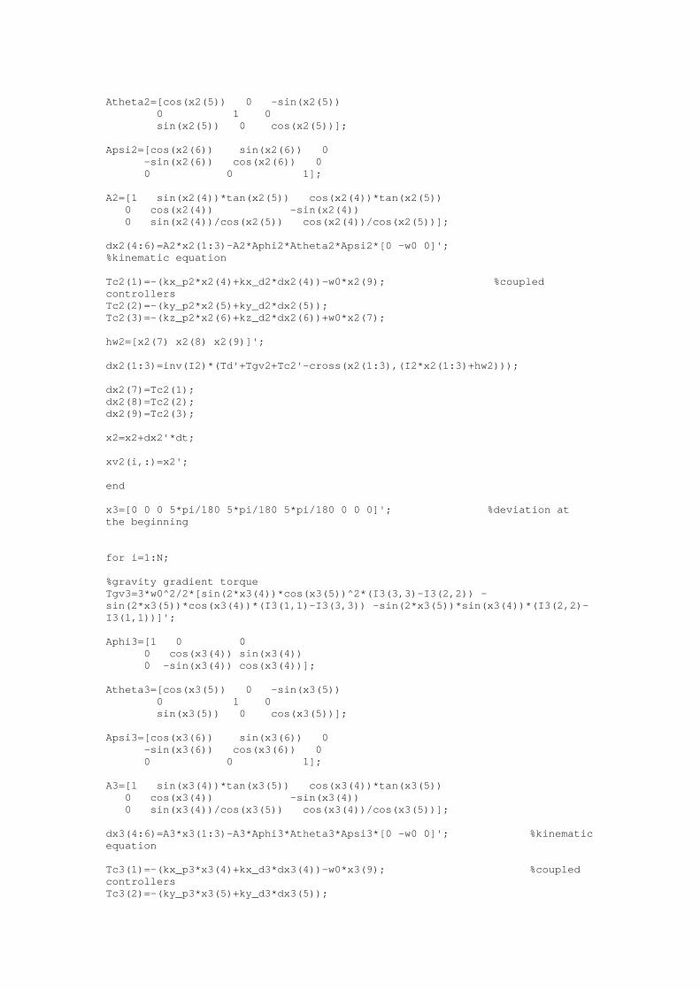
Atheta2=[cos(x2(5)) 0 -sin(x2(5)) 0 1 0 sin(x2(5)) 0 cos(x2(5))]; Apsi2=[cos(x2(6)) sin(x2(6)) 0 -sin(x2(6)) cos(x2(6)) 0 0 0 1]; A2=[1 sin(x2(4))*tan(x2(5)) cos(x2(4))*tan(x2(5)) 0 cos(x2(4)) -sin(x2(4)) 0 sin(x2(4))/cos(x2(5)) cos(x2(4))/cos(x2(5))]; dx2(4:6)=A2*x2(1:3)-A2*Aphi2*Atheta2*Apsi2*[0 -w0 0]'; %kinematic equation Tc2(1)=-(kx_p2*x2(4)+kx_d2*dx2(4))-w0*x2(9); %coupled controllers Tc2(2)=-(ky_p2*x2(5)+ky_d2*dx2(5)); Tc2(3)=-(kz_p2*x2(6)+kz_d2*dx2(6))+w0*x2(7); hw2=[x2(7) x2(8) x2(9)]'; dx2(1:3)=inv(I2)*(Td'+Tgv2+Tc2'-cross(x2(1:3),(I2*x2(1:3)+hw2))); dx2(7)=Tc2(1); dx2(8)=Tc2(2); dx2(9)=Tc2(3); x2=x2+dx2'*dt; xv2(i,:)=x2'; end x3=[0 0 0 5*pi/180 5*pi/180 5*pi/180 0 0 0]'; %deviation at the beginning for i=1:N; %gravity gradient torque Tgv3=3*w0^2/2*[sin(2*x3(4))*cos(x3(5))^2*(I3(3,3)-I3(2,2)) -sin(2*x3(5))*cos(x3(4))*(I3(1,1)-I3(3,3)) -sin(2*x3(5))*sin(x3(4))*(I3(2,2)-I3(1,1))]'; Aphi3=[1 0 0 0 cos(x3(4)) sin(x3(4)) 0 -sin(x3(4)) cos(x3(4))]; Atheta3=[cos(x3(5)) 0 -sin(x3(5)) 0 1 0 sin(x3(5)) 0 cos(x3(5))]; Apsi3=[cos(x3(6)) sin(x3(6)) 0 -sin(x3(6)) cos(x3(6)) 0 0 0 1]; A3=[1 sin(x3(4))*tan(x3(5)) cos(x3(4))*tan(x3(5)) 0 cos(x3(4)) -sin(x3(4)) 0 sin(x3(4))/cos(x3(5)) cos(x3(4))/cos(x3(5))]; dx3(4:6)=A3*x3(1:3)-A3*Aphi3*Atheta3*Apsi3*[0 -w0 0]'; %kinematic equation Tc3(1)=-(kx_p3*x3(4)+kx_d3*dx3(4))-w0*x3(9); %coupled controllers Tc3(2)=-(ky_p3*x3(5)+ky_d3*dx3(5));

Tc3(3)=-(kz_p3*x3(6)+kz_d3*dx3(6))+w0*x3(7); hw3=[x3(7) x3(8) x3(9)]'; dx3(1:3)=inv(I3)*(Td'+Tgv3+Tc3'-cross(x3(1:3),(I3*x3(1:3)+hw3))); dx3(7)=Tc3(1); dx3(8)=Tc3(2); dx3(9)=Tc3(3); x3=x3+dx3'*dt; xv3(i,:)=x3'; end figure(1) hold on title('w_x') plot(xv1(:,1)*180/pi,'-b') plot(xv2(:,1)*180/pi,'-r') plot(xv3(:,1)*180/pi,'-g') legend('launch, full tanks', 'solar array deployed, full tanks', 'solar array and lander deployed, tanks empty') xlabel ('time [20 sec]') ylabel('w_x [degrees/20 sec]') hold on figure(2) hold on title('w_y') plot(xv1(:,2)*180/pi,'-b') plot(xv2(:,2)*180/pi,'-r') plot(xv3(:,2)*180/pi,'-g') legend('launch, full tanks', 'solar array deployed, full tanks', 'solar array and lander deployed, tanks empty') xlabel ('time [20 sec]') ylabel('w_y [degrees/20 sec]') hold on figure(3) hold on title('w_z') plot(xv1(:,3)*180/pi,'-b') plot(xv2(:,3)*180/pi,'-r') plot(xv3(:,3)*180/pi,'-g') legend('launch, full tanks', 'solar array deployed, full tanks', 'solar array and lander deployed, tanks empty') xlabel ('time [20 sec]') ylabel('w_z [degrees/20 sec]') hold on figure(4) hold on title('phi') plot(xv1(:,4)*180/pi,'-b') plot(xv2(:,4)*180/pi,'-r') plot(xv3(:,4)*180/pi,'-g') legend('launch, full tanks', 'solar array deployed, full tanks', 'solar array and lander deployed, tanks empty') xlabel ('time [20 sec]') ylabel('phi [degrees]') hold on figure(5) hold on title('theta') plot(xv1(:,5)*180/pi,'-b')

plot(xv2(:,5)*180/pi,'-r') plot(xv3(:,5)*180/pi,'-g') legend('launch, full tanks', 'solar array deployed, full tanks', 'solar array and lander deployed, tanks empty') xlabel ('time [20 sec]') ylabel('theta [degrees]') hold on figure(6) hold on title('chi') plot(xv1(:,6)*180/pi,'-b') plot(xv2(:,6)*180/pi,'-r') plot(xv3(:,6)*180/pi,'-g') legend('launch, full tanks', 'solar array deployed, full tanks', 'solar array and lander deployed, tanks empty') xlabel ('time [20 sec]') ylabel('chi [degrees]') hold on figure(7) hold on title('momentum bias flywheel x') plot(xv1(:,7),'-b') plot(xv2(:,7),'-r') plot(xv3(:,7),'-g') legend('launch, full tanks', 'solar array deployed, full tanks', 'solar array and lander deployed, tanks empty') xlabel ('time [20 sec]') ylabel('momentum bias flywheel x [Nms]') hold on figure(8) hold on title('momentum bias flywheel y ') plot(xv1(:,8),'-b') plot(xv2(:,8),'-r') plot(xv3(:,8),'-g') legend('launch, full tanks', 'solar array deployed, full tanks', 'solar array and lander deployed, tanks empty') xlabel ('time [20 sec]') ylabel('momentum bias flywheel y [Nms]') hold on figure(9) hold on title('momentum bias flywheel z') plot(xv1(:,9),'-b') plot(xv2(:,9),'-r') plot(xv3(:,9),'-g') legend('launch, full tanks', 'solar array deployed, full tanks', 'solar array and lander deployed, tanks empty') xlabel ('time [20 sec]') ylabel('momentum bias flywheel z [Nms]') hold on

The results of the simulation: The results of the simulation are presented in the following graphs. The graphs represent the nine
components of the x-vector [ ]Tzyxzyx hhhx χθφωωω=
In the beginning, we stated a maximum allowable deviation of θ = 0.050 which is the most restricted requirement. The requirement is with reference to the lander ejection. In the simulation a linearized theory has been used. That is why the angles are kept small. The beginning deviation vector is set to x0 = [ 0 0 0 50 50 50 0 0 0 ]T. In Figure H.1 and Figure H.3, the angular velocities ωx and ωy of the satellite with respect to the inertial reference frame are nearly zero. This stays within an acceptable margin. In Figure H.2 the angular velocity ωy of the orbiter is –0.05, which is exactly the angular velocity needed for keeping the payload faced to the surface of the Moon during the whole orbit. Figure H.4, H.5 and H.6 show the angles φ, θ and χ which are the angles between the body reference frame and the orbit reference frame of the satellite. The angles stay within an allowable margin of θ = 0.28970
. Figure H.7 and H.9 show a cyclic change of angular momentum of the reaction wheels x and z. The magnitude of the angular momentum doesn't exceed the maximum allowable angular momentum of the reaction wheels (section 9.3.1) which is 12 Nms. The angular momentum of the reaction wheel y is shown in Figure H.8. The absolute value of the angular momentum rises continually as the angular rate ωy stays 0.050 per second. At a certain moment the wheels angular momentum will exceed -12 Nms and a momentum dumping will have to take place. This momentum dumping takes place every 45 hours (+/- 1.9 days).
Figure H.1: ωωx versus time

Figure H.2: ωωy versus time
Figure H.3: ωωz versus time
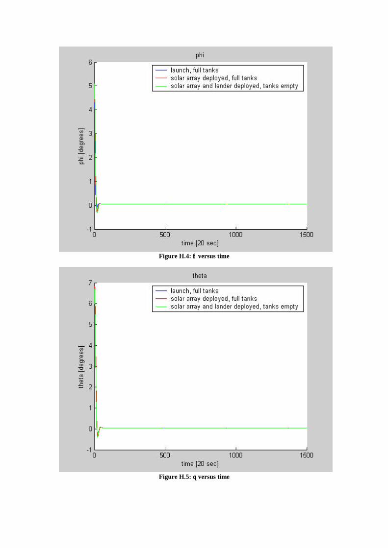
Figure H.4: φφ versus time
Figure H.5: θθ versus time

Figure H.6: χχ versus time
Figure H.7: hx versus time

Figure H.8: hy versus time
Figure H.9: hz versus time

The input variables of the simulation programme are: θ = 0.050 ω0 = 0.050 In the simulation programme the following mass moments of inertia have been used: Ixx total launch, full tanks 393,1807 solar array deployed, full tanks 649,5643 solar array and lander deployed, tanks empty 617,9768 Iyy total launch, full tanks 664,8227 Solar array deployed, full tanks 669,0731 Solar array and lander deployed, tanks empty 332,996 Izz total Launch, full tanks 691,2049 Solar array deployed, full tanks 953,9716 Solar array and lander deployed, tanks empty 695,9445 However, when the solar arrays turn around the Y-axis, the mass moments of inertia will change a little bit. This has been neglected. In a future study of the MiMiR mission the mass moments of inertia will have to be calculated for all positions of the solar arrays

Appendix H2: The reaction wheel of the MiMiR Orbiter
Fig. H.11: TELDIX reaction wheel
Main Technical Data (TELDIX) RSI 12-75/60x Angular Momentum at Nominal Speed 12 Nms Operational Speed Range ± 6000 rpm Speed Limiter (EMF) < 7500 rpm Motor Torque over full Speed Range ± 75 mNm Loss Torque (max.) < 20 mNm Dimensions: - Diameter 247 mm - Height 85 mm - Mass < 4.85 kg Power Consumption: - Steady State at Nominal Speed < 20 W - Max. Torque at Nominal Speed < 90 W Power Interface: - Supply Voltage 24 to 51 VDC - Input Current < 3.75 A - Galvanic Isolation between Primary Return and Secondary Return - Preceeding Stage – On/Off Relay Signal Interface: - Torque Command & Sign Analog/bi-level - Speed Measurement & Sign Digital/bi-level - Motor Torque ™ Analog - Thermistor for Temperature Measurement - On/Off Status bi-level - On/Off Command pulses Environmental Conditions: - Qualification/Protoflight Temperature - 25 … + 75 °C (synthetic oil) - Acceptance Temperature - 20 … + 70 °C (synthetic oil) - Survival/Non-operating - 40 … + 75 °C (synthetic oil) Lifetime > 15 years (in-orbit)
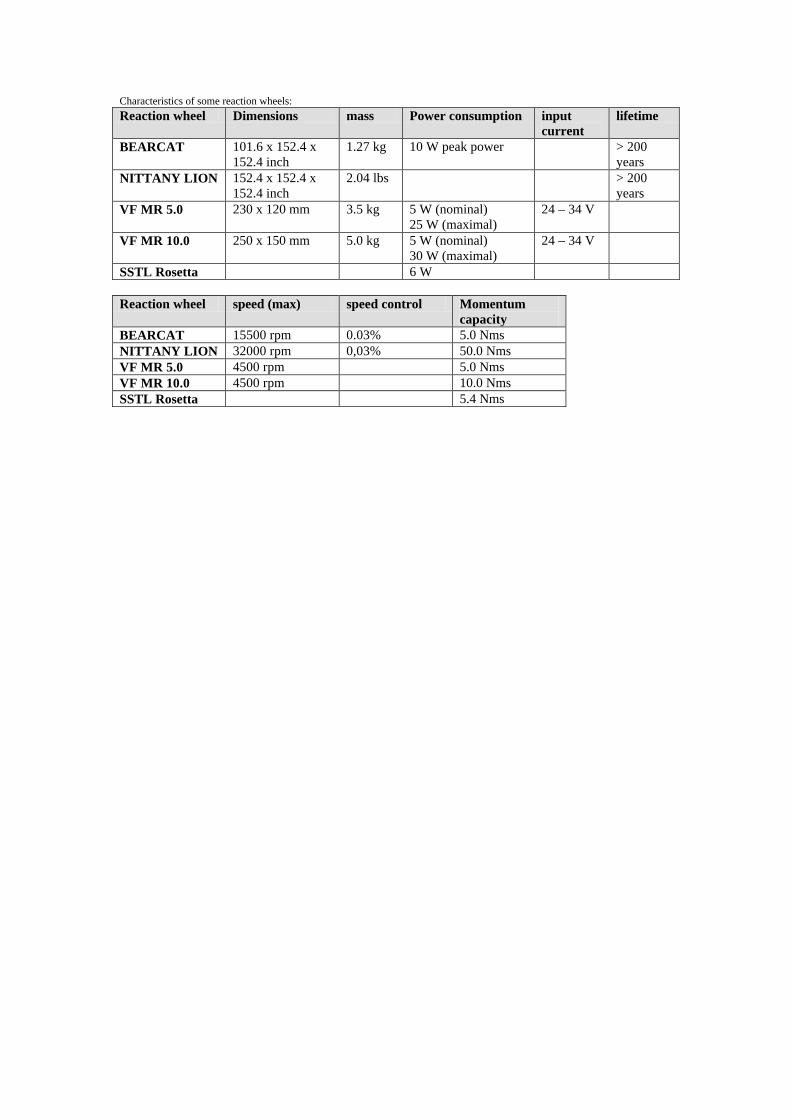
Characteristics of some reaction wheels:
Reaction wheel Dimensions mass Power consumption input current
lifetime
BEARCAT 101.6 x 152.4 x 152.4 inch
1.27 kg 10 W peak power > 200 years
NITTANY LION 152.4 x 152.4 x 152.4 inch
2.04 lbs > 200 years
VF MR 5.0 230 x 120 mm 3.5 kg 5 W (nominal) 25 W (maximal)
24 – 34 V
VF MR 10.0 250 x 150 mm 5.0 kg 5 W (nominal) 30 W (maximal)
24 – 34 V
SSTL Rosetta 6 W Reaction wheel speed (max) speed control Momentum
capacity BEARCAT 15500 rpm 0.03% 5.0 Nms NITTANY LION 32000 rpm 0,03% 50.0 Nms VF MR 5.0 4500 rpm 5.0 Nms VF MR 10.0 4500 rpm 10.0 Nms SSTL Rosetta 5.4 Nms

Appendix H3: Sun sensor for the MiMiR Orbiter
Figure H.12: Sun sensor
Accuracy Better than +/- 0.2 degrees on boresight for GEO missions (albedo degrades accuracy in LEO). Output at offset positions is affected by seasonal variatisons in solar intensity (+/- 3%), temperature variations (up to 10% BOL, 25% EOL over whole range of operating temperatures), and radiation degradation of silicon cells (up to 20% in GEO telecom missions). Field of view Hemispherical, typically +/- 97 degrees about boresight. Power consumption No input power required. Electrical output In current mode 0 – 40 mA. In voltage mode 0 – 250 mV. Output can be of single photocells or of combinations of single cells (balance, sum). Operating temperature –80 C to +80 C. Mass/dimensions 0.155 kg; 110 x 110 x 28 mm without connector, alignment cube, grounding stud or specific baffling. Reliability Depend strongly on output arrangement (single cell or combination output) and philosophy with regard to redundancy; in SAS for GEO application outputs are redundant; in SAS for LEO application only single-cell type of output is redundant; failure probability for single cell voltage output 2.4 x 10⁻⁴ worst case (+80 C) per year mission duration.

Qualification status Fully qualified sensor; SAS sensors were designed for the Rosetta mission and the Mars Express satellite. Provider Developed by TPD/TNO Delft for the Rosetta satellite and the Mars Express satellite.
Appendix H4: Star tracker HD-1003 NEAR NASA FY
94 Pluto Flyby
NASA Deep Space 1
Oersted Satellite Tracker
Clementine
Application Mass (kg) Power (W) FOV (°°) Imager Format (pixels) Cooling Sensitivity (M) Quantisation (bits) Update rate (hz) Noise Comments
Antenna pointing - - - TI CCD 1000x510 yes 6 - - - 2 trackers, mechanical windowing, integration time 0.0625-2s, self test LED
Commercial 4 9 8 or 20 CCD - - 4.7 or 6.0 - 10 or 4 - tracks 6 stars
Attitude control, instrument pointing - - 20 CCD 512x512 -25° C 4.5 10 5 - tracks 5 stars
Sole attitude, control system 2 3.5 8x8 CCD 1025x512 yes 6 - 2.5 - local filtering, frame buffer, windowing on buffer
- - - 0.8 CCD 1024x1024 - 13 12 - 40 motion compensation software, integration time up to 100 s
ST and WFOV science camera and Cherenkov detector 1.4 4.5 22x16 interline CCD - - - - - - recalibrates for radiaction degradation
0.29 4.5 29x43 CCD 576x384 10 °C 4.5 8 10 90+60
Characteristics of some other star sensors:
Star sensors Dimensions mass power consumption
input current
lifetime
VF STC 1 320 x 320 x 160 mm
3.2 kg 10.2 W 24 – 28 V
15 years
VF STC 2 280 x 280 x 225 mm
3.4 kg 24 – 28 V
15 years
SED12 Star L = 231 mm; 8.4 kg 13 – 19 W 22 – 39

Tracker diameter = 141 mm and 270 x 215 x 180 mm
V
SED16 Star Tracker
278 x 158 x 147 mm
8 W 16 – 55 V
Clementine Star tracker
0.29 kg 4.5 W
Star sensors
FOV
Accuracy
Data Updating Frequency
star catalog
search time
Maximum star magnitude
VF STC 1 8 degrees circular
x,y: 3 arcsec, z: 15 arcsec
10.2 W 8500 2 sec (initial: 30 sec)
+8.5
VF STC 2 x,y: 3 arcsec, z: 22 arcsec
5000 2 sec (initial: 30 sec)
+6
SED12 Star Tracker
2 Hz 22 – 39 V -4.5 to +8.0
SED16 Star Tracker
x,y: 3 to 14 arcsec, z: 10 to 30 arcsec
10 Hz 16 – 55 V
Clementine Star tracker
29 x 43 degrees Instantaneous Field of View: 1.3 mrad
10 Hz 600 (stellar compass computer programme)
+4.5

Figure H.13: Star tracker

Appendix H5: Simulation programme for the MiMiR lander 'Cornetto' A simple simulation programme has been written for the attitude control of the lander 'Cornetto', for a turn around the x-axis. The graphs show the angle and angular velocity of the lander during a thruster burn of 10 seconds. The applied thrust is 0.5 Newton. The input moments of inertia are Ix = 25.33397 (full tanks) and Ix = 13.90064 (tanks empty). The results for a turn around the y-axis will not differ much from the results of the x-axis, as the mass moments of inertia do not differ much. (Iy = 26.04146 (full tanks) and Iy = 14.60813 (tanks empty)). The simulation about the z-axis is not done, as this manoeuvre is not necessary in the first point of view. Also translational motions are not considered. In a future MiMiR mission study this will have to be done.
Figure H.14: Angle of lander between body axis and reference axis

Figure H.15: Angular velocity of the lander
The simulation program: clear all; close all; clc; x1 = 0; x2 = 0; xfl1 = 0; xfl2 = 0; Ix1 = 25.33397; %full tanks Iy1 = 26.04146; Iz1 = 38.30876; Ix2 = 13.90064; %tanks empty Iy2 = 14.60813; Iz2 = 21.15876; a = 0.35; %distance between the thrusters and the c.g. F1 = 0.5; %thrust of thruster 1 F2 = 0.5; %thrust of thruster 2 F3 = 0.5; %thrust of thruster 3 F4 = 0.5; F5 = 0.5; F6 = 0.5; %assume you want a turn around the x-axis, using only 1 thruster (the translational motion is not considered) then: F2 = 0; F3 = 0; F4 = 0; F5 = 0; F6 = 0; xdfl1=(F1)*a/Ix1

dt=1; tf=10; %total time the thrusters are switched on N=tf/dt; opslagxfl1 = [xfl1]; opslagx1 = [x1]; opslagt1 = [0]; for i=1:N; x1 = (1/2)*xdfl1*dt^2 + xfl1*dt + x1 xfl1 = xdfl1*dt + xfl1 opslagxfl1 = [opslagxfl1,xfl1]; opslagx1 = [opslagx1,x1]; opslagt1 = [opslagt1,i]; end xdfl2=(F1)*a/Ix2 dt=1; tf=10; %total time the thrusters are switched on N=tf/dt; opslagxfl2 = [xfl2]; opslagx2 = [x2]; opslagt2 = [0]; for i=1:N; x2 = (1/2)*xdfl2*dt^2 + xfl2*dt + x2 xfl2 = xdfl2*dt + xfl2 opslagxfl2 = [opslagxfl2,xfl2]; opslagx2 = [opslagx2,x2]; opslagt2 = [opslagt2,i]; end figure(1) hold on title('x') plot(opslagt1,opslagx1*180/pi,'-b') plot(opslagt2,opslagx2*180/pi,'--r') xlabel ('time [sec]') ylabel('angle x [degrees]') legend('full tanks','tanks empty',0) figure(2) hold on title('xfl') plot(opslagt1,opslagxfl1*180/pi,'-b') plot(opslagt2,opslagxfl2*180/pi,'--r') xlabel ('time [sec]') ylabel('angular velocity [degrees/sec]') legend('full tanks','tanks empty',0)

Appendix H6: Specifications of the attitude control thrusters of the 'Cornetto' Lander
Figure H.16 : Attitude control thruster for Cornetto-lander
CHT0.5 Thruster Engine statistics
Specification Value Thrust 0.5N Power (kW/HP) 0.55/0.75 Propellant Hydrazine Isp 2230 m/s Chamber Pressure 22 bar Weight 195 g Length 113 mm Nozzle Diameter 4.8 mm

Appendix I

EARTH GTO inclination 51,8 degmhu - Earth 398600 km^3/s^2 alt. apogeum 35786 kmRadius 6378 km alt. perigeum 200 km
radius apogeum 42164 kmradius perigeum 6578 km
MOON a 24371 kmRadius 1737,4 km e 0,730089mhu - Moon 4902,8 km^3/s^2 V apogeum 1597,379 m/sEarth - Moon (=a) 384400 km V perigeum 10238,96 m/se 0,0549 Period GTO 37863,54 sapogeum 405503,56 km 10,52 h
perigeum 363296,44 km TRANSFERmax inclination 28,65 deg radius apogeum 384400 km Delta V1 676,7541 m/smin inclination 18,35 deg radius perigeum 6578 kmV apogeum 963,851645 m/s a 195489 kmV perigeum 1075,83018 m/s e 0,966351
average 1019,84091 V apogeum 186,7939 m/sV perigeum 10915,72 m/sV relative to moon -833,047 m/s (average)
Transfer time 4,30E+05 s
LUNAR CAPTURE 4,98 days
V apogeum - arrival 186,793917 m/s INSERTIONDelta inclinatie (worst case) 33,45 deg #1: 12h ORBIT Period 12 hDelta inclinatie (best case) 23,15 deg 43200 s
Delta V inclination 61,8784139 m/s alt. perigeum 100 km
Delta V inclination 30,0817525 m/s alt. apogeum 8710,355 kmV infinite relative to moon 0,83304699 km/s radius perigeum 1837,4 km
alt. perigeum 100 km radius apogeum 10447,76 km
radius perigeum (=r3) 1837,4 km a 6142,578 kmB 5416,46405 km e 0,700875Velocity first 2,45573587 km/s V apogeum 374,6598 ms to 3,5h orbitperigeum passage V perigeum 2,130377 km/s
Delta V2-1 325,3592 m/s
gravity losses 32,53592 m/s
total 357,8951 m/s

#2: 3,5h ORBIT #3: FINAL ORBIT DEPLOYMENT LANDERPeriod 3,5 h Period 1,963 h Period 1,899425 h
12600 s 7067,460 s 6837,93 salt. perigeum 100 km alt. perigeum 100 km alt. Perigeum 20 kmalt. apogeum 1828,24 km alt. apogeum 100 km alt. Apogeum 100 kmradius perigeum 1837,4 km radius perigeum 1837,4 km radius perigeum 1757,4 kmradius apogeum 3565,64 km radius apogeum 1837,4 km radius apogeum 1837,4 kma 2701,52 km a 1837,4 km a 1797,4 km
e 0,319864 e 0 e 0,022254from 12h orbit V apogeum 967,05 m/s V apogeum 1,6635 km/s V perigeum 1,6888 km/s
V perigeum 1,87666 km/s V perigeum 1,6635 km/s V apogeum 1,61523 km/s
Delta V2-2 253,72 m/s Delta V2-3 243,16 m/s Delta V 18,279 m/sgravity losses 25,372 m/s gravity losses 24,316 m/s ascend+descent 36,558 m/s
margin 10 m/s
Total 279,092 m/s Total 267,476 m/s Total 46,558 m/s
OTHER
Mid-Course Correction 2x 50=100 m/s TOTAL Delta V 1243 m/sContingency 30 m/s (not including LTO insertion)
Orbit Keeping 100 m/s Fuel 340,7 kg
Dry mass bus 500 kglander 130 kgPayload 70 kgTotal Dry Mass 700 kg2% residual 7,8361 kg
TOTAL Weight 1049 kg

Appendix I2: The LTO calculator The optimization of April 28th 2005 is treated below as an example. For a launch at 3.50 a.m., the LTO calculator gives as result:
• ∆V1 for injection from GTO into LTO = 657.05 m/s • ∆V2 for insertion into LLO = 842.62 m/s _____________________________________________________ • ∆Vtotal = 1499.67 m/s • azimuth = 47 degrees • declination = -9 degrees
I2.1 Output graphs The following figures I.1-I.4 show the orbit and the position of the Moon in respectively 3D view, X-Y view, X-Z view and Y-Z. The LTO calculator stops the computations when the orbiter reaches the Moon's sphere of influence.
Figure I..1 3D view of the Hohmann transfer on April 28th

figure I..2: XY view of the Hohmann transfer on April 28th
Figure I..3: XZ view of the Hohmann transfer on April 28th

Figure I..3: YZ view of the Hohmann transfer on April 28th
I2.2 Output Data MJD launch = 1.94499305555555E+0003 MJD first perigeum passage = 1.94587931712962E+0003 MJD2000 = 1.94759051712962E+0003 Earth orbit: semi-major axis = 2.43711440000000E+0004 km eccentricity = 7.30084726428928E-0001 inclination = 5.18000000000000E+0001 deg RAAN = 0.00000000000000E+0000 deg argument of perigeum = 180 deg true anomaly = 0 deg dV1 = 6.57048200000000E-0001 m/s T phase = 1.71120000000000E+0000 days Transfer orbit: R0 = (-6.57814400000000E+0003, 4.98167351288071E-0013, 6.33057781724180E-0013) km V0 = (-1.33431911529032E-0015,-6.73811743999236E+0000,-8.56261990780670E+0000) km/s Moon encounter number: 1 t = 2.92886200443815E+0000 days MJD2000 = 1.95051937913406E+0003 days Delta_V = 8.50833618606235E-0001 km/s DV_tot = 1.50788181860623E+0000 km/s R with respect to the Moon = (-6.48160528407159E+0004, 5.72864438955057E+0003, 8.41782899203932E+0003) km Velocity with respect to the Moon = ( 2.72498620927003E-0001,-8.72532155770688E-0001,-1.07716468969025E-0002) km

Perilune passage parameters (North bound): semi-major axis = -5.86679338250724E+0003 km eccentricity = 1.31328868773192E+0000 inclination = 9.00000000000000E+0001 deg RAAN = 1.07343992947836E+0002 deg argument of perigeum = 1.40267086781589E+0002 deg true anomaly = 0.00000000000000E+0000 deg Perilune passage parameters (South bound): semi major axis = -5.86679338250724E+0003 km eccentricity = 1.31328868773192E+0000 inclination = 9.00000000000000E+0001 deg RAAN = 2.87343992947836E+0002 deg argument of perigeum = 3.18916806978097E+0002 deg true anomaly = 0.00000000000000E+0000 deg Moon encounter number: 2 t = 2.92886200443815E+0000 days MJD2000 = 1.95051937913406E+0003 days Delta_V = 8.50833618606235E-0001 km/s Delta V total = 1.50788181860623E+0000 km/s R with respect to the Moon = (-6.48160528407159E+0004, 5.72864438955057E+0003, 8.41782899203932E+0003) km Velocity with respect to the Moon = ( 2.72498620927003E-0001,-8.72532155770688E-0001,-1.07716468969025E-0002) km Perilune passage parameters (North bound): semi major axis . = -5.86679338250724E+0003 km eccentricity = 1.31328868773192E+0000 inclination = 9.00000000000000E+0001 deg RAAN = 1.07343992947836E+0002 deg argument of perigeum = 1.40267086781589E+0002 deg tr.an. = 0.00000000000000E+0000 deg Perilune passage parameters (South bound): s.m.a. = -5.86679338250724E+0003 km ecc. = 1.31328868773192E+0000 incl. = 9.00000000000000E+0001 deg RAAN = 2.87343992947836E+0002 deg arg.pg = 3.18916806978097E+0002 deg true anomaly = 0.00000000000000E+0000 deg second delta_V = 0.00000000000000E+0000 km/s MJD2000 = 1.95174873772594E+0003 days t = 3.59270259521373E+0005 sec R = ( 3.31150894304260E+0005, 4.10812906485190E+0003, 5.18520273150102E+0003) km V = ( 1.06452813173261E-0003, 1.74309108079410E-0001, 1.71454556058164E-0001) km dV2 = (-0.00000000000000E+0000, 0.00000000000000E+0000, 0.00000000000000E+0000) km/s (inertial)

Appendix J
Appendix J1: Lander - Orbiter Uplink budget Lander-Orbiter UplinkLink Margin 28,17 dB
Transmitter
Transmitter power 5 W 6,99 dBTransmitter line loss 1 dB -1,00 dB
Transmitter helix
Frequency 2250 MHzBeamwidth 70 degWavelength 0,133333 mC (from 9.3.1.2) 0,136 mHelix diameter 0,04329 mHelix length 0,070721 mAntenna gain 7,72 dB
Max distance 230 kmSpace Loss -146,73 dBSystem noise temperature 500 K -26,99 dB
Boltzmann 228,60 dB
Receiver helixFrequency 2250 MHzBeamwidth 70 degWavelength 0,133333 mC 0,136 mHelix diameter 0,04329 mHelix length 0,070721 mAntenna gain 7,72 dB
ReceiverReceiver LN Amp 0 dBi 0,00 dBReceiver line loss 1 dB -1,00 dB
Bandwidth 8 kbps -39,13 dBImplementation loss 2 dB -2,00 dBRequired E_b/N_0 6 dB -6,00 dB
Link margin 28,17 dB

Appendix J2: Lander – Orbiter downlink budget Lander-Orbiter downlinkLink Margin 1,28 dB
Transmitter
Transmitter power 5 W 6,99 dBTransmitter line loss 1 dB -1,00 dB
Transmitter helix
Frequency 2200 MHzBeamwidth 70 degWavelength 0,136364 mC 0,136 mHelix diameter 0,04329 mHelix length 0,075653 mAntenna gain 7,72 dB
Max distance 230 kmSpace Loss -146,53 dBSystem noise temperature 500 K -26,99 dB
Boltzmann 228,60 dB
Receiver helixFrequency 2200 MHzBeamwidth 70 degWavelength 0,136364 mC 0,136 mHelix diameter 0,04329 mHelix length 0,075653 mAntenna gain 7,72 dB
ReceiverReceiver LN Amp 0 dBi 0,00Receiver line loss 1 dB -1,00
Bandwidth 4096 kbps -66,23Implementation loss 2 dB -2,00Required E_b/N_0 6 dB -6,00
Link margin 1,28

Appendix J3: Earth – Orbiter Uplink budget
Earth-Orbiter UplinkLink Margin 2,25 dB
Transmitter
Transmitter power 25 W 13,98 dBTransmitter line loss 1 dB -1,00 dB
Transmitter dish
Frequency 2250 MHzBeamwidth n/aWavelength n/aC n/aHelix diameter n/aHelix length n/aAntenna gain 26,00 dB
Max distance 400000 kmSpace Loss -211,53 dBSystem noise temperature 500 K -26,99 dB
Boltzmann 228,60 dB
Receiver helixFrequency 2250 MHzBeamwidth 14,6 degWavelength 0,133333 mC 0,164 mHelix diameter 0,052203 mHelix length 1,117968 mAntenna gain 21,33 dB
ReceiverReceiver LN Amp 0 dBi 0,00 dBReceiver line loss 1 dB -1,00 dB
Bandwidth 8 kbps -39,13 dBImplementation loss 2 dB -2,00 dBRequired E_b/N_0 6 dB -6,00 dB
Link margin 2,25 dB

Appendix J4: Earth – Orbiter downlink budget
Earth-Orbiter downlinkLink Margin 2,36 dB
Transmitter
Transmitter power 5 W 6,99 dBTransmitter line loss 1 dB -1,00 dB
Transmitter helix
Frequency 2200 MHzBeamwidth 14,6 degWavelength 0,136364 mC 0,164 mHelix diameter 0,052203 mHelix length 1,195939 mAntenna gain 21,33 dBPointing error 3 dB -3,00 dBMax distance 400000 kmSpace Loss -211,34 dBSystem noise temperature n/a K
Boltzmann 228,60 dB
Receiver helixFrequency 2200 MHzBeamwidth n/aWavelength n/aC n/aHelix diameter n/aHelix length n/aAntenna gain 26,00 dB
ReceiverReceiver LN Amp (incl. noise) 10 dBi 10,00 dBReceiver line loss 1 dB -1,00 dB
Bandwidth 4096 kbps -66,23 dBImplementation loss 2 dB -2,00 dBRequired E_b/N_0 6 dB -6,00 dB
Link margin 2,36 dB

Appendix J5: Design Options Tree
For the selection of one of the antennas on the orbiter, a design options tree has been used. This antenna is to be used for the link to the earth, and it is preferable to have a high gain antenna. Having selected the S-band as the frequency range for communicating, it is possible to make the first decision: whether a dish or helix antenna can be used. These are the only two types of antennas useable for these kinds of links. After calculating the dimensions and masses which are needed for sending and receiving data to and from the ground stations, it turned out a dish antenna with an acceptable gain cannot fit on the lander. The second decision to be made in this phase was whether to use a rigid wide beam helix, or a pointable narrow beam antenna. Using a wide beam antenna has the advantage that it is short, thus lightweight, and doesn’t have too much influence on the moment of inertia of the lander. Furthermore, it doesn’t need a pointing mechanism, which saves a lot of weight. The big disadvantage of this wide beam antenna though, is that its gain is much lower. In fact, it is so low that it consumes too much power. So, despite its disadvantages, the narrow beam antenna has been chosen as the antenna to communicate with the ground stations on Earth.
Antenna on orbiter
Dish antenna Helix antenna
Pointable narrow beam antenna Rigid wide beam antenna

Appendix K
Appendix K: Details of the Temic Semiconductor TSC21020F processor BASIC BUILDING BLOCKS The reconfigurable modular on-board payload processing system will be made up of basic building blocks, sometimes to be complemented with application specific hardware. Important requirements as reduced power consumption, mass and volume, flexibility for introducing modern state of the art technology and scalability to allow enhancement of the performances were used while developing these building blocks. Several blocks, that can be either devices or modules, exist already while others are being developed. Devices. The kernel of the on-board processing system is the Digital Signal Processor (DSP), TSC21020F1. This is complemented by memory devices, high-speed interfaces, a DPC (DSP Peripheral Controller) and a lossless compression and CCSDS packetization device. The DSP is a radiation tolerant version of the Analog Devices ADSP–21020 32/40–Bit Floating–Point DSP. This version is called the TSC21020F and is manufactured by TEMIC Semiconductors. The product is pin and code compatible with the Analog Devices product, making system development straightforward and cost effective, because use can be made of existing development tools and algorithms. The main features of the TSC21020F are: • Clock frequency 20 MHz • 50 ns, 20 MIPS Instruction Rate, Single-Cycle Execution • 60 MFLOPS Peak, 40 MFLOPS Sustained Performance • 1024-Point Complex FFT Benchmark: 0.975 ms • 32-Bit Single-Precision and 40-Bit Extended-Precision IEEE Floating-Point Data Formats • 32-Bit Fixed-Point Formats, Integer and Fractional, with 80-Bit Accumulators • Multiply with Add & Subtract for FFT Butterfly Computation • Latch up immune • Total dose better than 100 Krad (Si) • SEU immunity better than 50 MeV/mg/cm 2 • Typical power consumption 1 W For the Solid-State Mass Memory modules either 64 or 256 Mbit commercial SDRAMs are used. High-speed interfaces are based on the SMCS3322 (Scalable Multi-channel Communication Subsystem implementing 3 x IEEE1355 links at 150 Mbps full duplex each) devices, of which light versions exist namely SMCS116 (lite), SMCSlite2. The DPC which is a DSP Peripheral Controller. For lossless compression the Packetizing Rice Data Compressor (PRDC) is available, which is a lossless compression ASIC for space-borne applications. The PRDC is compliant with CCSDS Lossless Data Compression Standard for sample widths up to 16 bits. An optional extension to the standard is implemented (can be disabled) to slightly improve the performance. In addition the PRDC provides packetizing and depacketizing functions for the compressed data according to ESA Packet Telemetry Standard (PSS-04-106).

Appendix L
Appendix L1: Power Breakdown Structure Orbiter
Subsystem Part Power [W] Payload HRSC 40.4
OMEGA 42 Neutron Spectrometer 3 Laser Altimeter 10 Gamma-ray Spectrometer 2
Propulsion 0 Attitude control and Navigation 36.525
Communications 12.175 Command and data handling 12.175
Thermal 12.175 Power 73.05
Structure 0 Total 243.5
Lander
Subsystem Part Power [W] Payload TDL 9 (1.5 each)
Raman Spectrometer 2.5 Microscopic Imager 10 Lamp 0.1 Nanokhod Rover 5 GPR 3 RSS/N 10 Permittivity Probe 0.1
Propulsion 0 Attitude control and Navigation 50
Communications 1.5 Command and data handling 15
Thermal 0 Power 0
Structure 0 Total 106.2
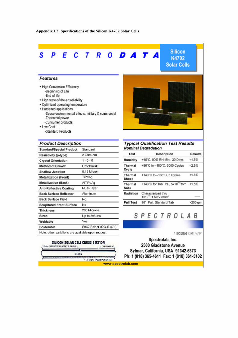
Appendix L2: Specifications of the Silicon K4702 Solar Cells


Appendix L3: Specifications of the ICR33600B Li-ion Cells Electrical Characteristics Nominal Voltage 3.6 V Rated Capacity 5.0 Ah Typical Capacity 5.0 Ah Physical Characteristics Height 60.1 ± 0.2mma Diameter 33.0 ± 0.1mm Mass (typical) 125 g Operating Conditions Discharge Temperature Range -30°C to +55°C Charge Temperature Range 0°C to 50°C Maximum current 5.0 A continuos/10 A pulse Charging method Constant current and constant voltage
1.5 A followed by 2 h at 4.2 V ± 0.05 V End (of discharge) Voltage 2.5 v End (of charge) Voltage 4.2 V ± 0.05 V AGM Batteries Ltd Culham Science Centre E1 Culham Abingdon OXON OX14 3ED United Kingdom Tel: +44 (0)1235 463064 Fax: +44 (0)1235 463400

Appendix M
Appendix M1: Thermal Characteristics and formulas No. Item Symbol Value Units Source Comment 1 Surface area of MiMiR A 16.0 m2
calculated 1,7x1,5x1,7
2 Diameter of sphere which equals MiMiR surface
D 2.25 m πD2 = 16 m2
3 Power dissipation QW 240 W 4 Altitude H 100 km 5 Direct Solar Flux Gs 1400 W/m2 6 Radius of Moon Rm 1737.4 km 7 Angular radius of Moon ρ 1.239358 8 Average albedo a 0.07 9 IR emittance Kapton ε 0.45-0.75 10 Absorptivity Kapton α 0.45 11 IR emittance Optical Solar
Reflectors ε 0.79
12 Absorptivity Optical Solar Reflectors
α 0.007
13 IR emittance white paint ε 0.9 14 Absorptivity white paint α 0.25 15 Worst case hot
temperature Tmax 335,65 K
16 Worst case cold temperature
Tmin 261,15 K
20 Radiator area based on worst case hot conditions
Ar 1,7m2
The computions made to derive the worst case hot and worst case cold conditions are based on the principle of conservation of energy:
emittedndissipatioIRalbedosolarp QQQQQdtdT
mc −+++= (14.1)
40 TAQSASASAk
dtdT
mc emittedIRndissipatioIRIRIRaassssp σεααα −+++= (14.2)

The surface area exposed to direct Solar Flux is effective equal to the cross-section of the sphere which equals the MiMiR-Orbiter surface. The effective exposed areas to Albedo and Moon Infrared are the half of the surface area of the sphere.
(14.3)
(14.4)
To determine an equilibrium temperature, the "steady-state temperature", the left side of equation (14.2) is is assumed to be zero.
0=−+++ emittedndissipatioIRalbedosolar QQQQQ (14.5)
This leaves:
4220
2
21
41
0 TDQSDSASDk IRndissipatioIRIRaasss σπεπααπα −+++= (14.5)
4
1
2
220
2
21
21
41
+++=
σπε
παπαπα
D
QSDSDSDkT
IR
ndissipatioIRIRasss
(14.6)
The solar constant S0, integrated solar irradiance at 1 AU, has been measured as 1371±5 W m –2. Taking into account the perihelion and aphohelion distances, a variation of the solar constant from 1418 W m –2 to 1326 W m –2 should be considered. In the calculations a value of 1400 W m –2 for the Solar constant at the Moon is used. The total Solar Albedo is seven percent of the direct Solar Flux. The assumption is made that the power dissipation is approximately equal to the power needed for operation. The available power is about 240 W. This value is used for a worst-case estimate temperature computation.
2
41
DAs π=
2
21
DAA IRa π==

Appendix M2: Matlab Single-Node computation The MATLAB m file and the calculated results are stated below. % Thermal Analysis - Space Mission Analysis and Design %assumed:-uniform energy dissipation over entire surface of the sphere % -no electrical generation on the spherical surface clear; close all; clc; %SMAD 11-13 % q_absorbed+q_dissipated-q_emitted=0;%energy balance used to estimate equilibrium temperature %SMAD 11-14 en 11-15 Gs_hot=1418; %solar constant [W/m^2] Gs_cold=1326; Gs_mean=1400; alfa_kapton=0.45; %solar absorptivity of sphere alfa_gold=0.299; epsilon_kapton = 0.45; %IR emissivity of sphere epsilon_gold=0.023; sigma=5.67*10^-8; %Stefan-Boltzmann constant [W*m^-2*K^-4] D=2.225; %diameter of spacecraft sphere H=100; %the altitude of the spacecraft Rm=1737.4; %radius of the moon rho =1.239358; %the angular radius of the Moon sin rho= Rm/Rm+H qImax=1123; %Moon IR emitted energy flux at the surface of the Moon qImin=43; %qI = [43 109.3 892 1123]; qImean=500; Ap=8; %projected area[m^2] Ar=8; %radiator area % Ka = 0.664+0.521*rho-0.203*rho^2 %absorbed energy q_absorbed_hot=Gs_hot*Ap*alfa_kapton; %[W] q_absorbed_cold=Gs_cold*Ap*alfa_kapton; %[W] %q_emitted=q_absorbed %q_emitted=epsilon*sigma*T^4*Ar %SMAD 11-18 GI_max=qImax*((Rm^2)/((H+Rm)^2)); %GI=Moon IR radiation flux at 100 km GI_min=qImin*((Rm^2)/((H+Rm)^2)); %SMAD 11-19 q_IR_max=GI_max*Ap*epsilon_kapton; %absorbed Moon infrared radiation on the bottom of the sphere q_IR_min=GI_min*Ap*epsilon_kapton; %SMAD 11-20 a=0.07; %Albedo of direct solar Qw=240 ; %[W],%electrical power dissipation,equal to needed power during operation q_solar=(0.25*Gs_hot*Ap*alfa_kapton) q_IR=(0.5*qImax*epsilon_kapton*(1-cos(rho))*Ap) q_albedo=(0.5*Gs_hot*a*alfa_kapton*(1-cos(rho))*Ap)

q_powerdissipation=(Qw) %temperature expressions according to SMAD Tmax_hot_kapton =(((0.25*Gs_hot*alfa_kapton)+(0.5*qImax*epsilon_kapton*(1-cos(rho)))+(0.5*Gs_hot*a*alfa_kapton*(1-cos(rho)))+(Qw/(pi*(D^2))))/(sigma*epsilon_kapton*2))^0.25; Tmax_mean_kapton =(((0.25*Gs_hot*alfa_kapton)+(0.5*qImean*epsilon_kapton*(1-cos(rho)))+(0.5*Gs_hot*a*alfa_kapton*(1-cos(rho)))+(Qw/(pi*(D^2))))/(sigma*epsilon_kapton*2))^0.25; Tmax_hot_gold =(((0.25*Gs_hot*alfa_gold)+(0.5*qImax*epsilon_gold*(1-cos(rho)))+(0.5*Gs_hot*a*alfa_gold*(1-cos(rho)))+(Qw/(pi*(D^2))))/(sigma*epsilon_gold*2))^0.25; Tmax_cold =(((0.25*Gs_cold*alfa_kapton)+(0.5*qImax*epsilon_kapton*(1-cos(rho)))+(0.5*Gs_cold*a*alfa_kapton*(1-cos(rho)))+(Qw/(pi*(D^2))))/(sigma*epsilon_kapton*2))^0.25; q_emmitted=(sigma*epsilon_kapton*Ap*(Tmax_hot_kapton^4)); Tmin_IR_min = ((0.5*qImin*epsilon_kapton*(1-cos(rho))+(Qw/(pi*(D^2))))/(sigma*epsilon_kapton))^0.25; Tmin_IR_mean = ((0.5*qImean*epsilon_kapton*(1-cos(rho))+(Qw/(pi*(D^2))))/(sigma*epsilon_kapton))^0.25; Tmin_IR_max = ((0.5*qImax*epsilon_kapton*(1-cos(rho))+(Qw/(pi*(D^2))))/(sigma*epsilon_kapton))^0.25; Tmax=((q_solar+q_IR+q_albedo+Qw/(pi*(D^2)))/(sigma*epsilon_kapton*2*Ap))^0.25 %resulting equilibrium worst-case hot temperature Tmin=((q_IR+Qw/(pi*(D^2)))/(sigma*epsilon_kapton*2*Ap))^0.25 %resulting equilibrium worst-case cold temperature The output: q_solar = 1.2762e+003 q_IR = 1.3636e+003 q_albedo = 120.5288 q_powerdissipation = 240 Tmax = 287.1559 Tmin = 241.0832
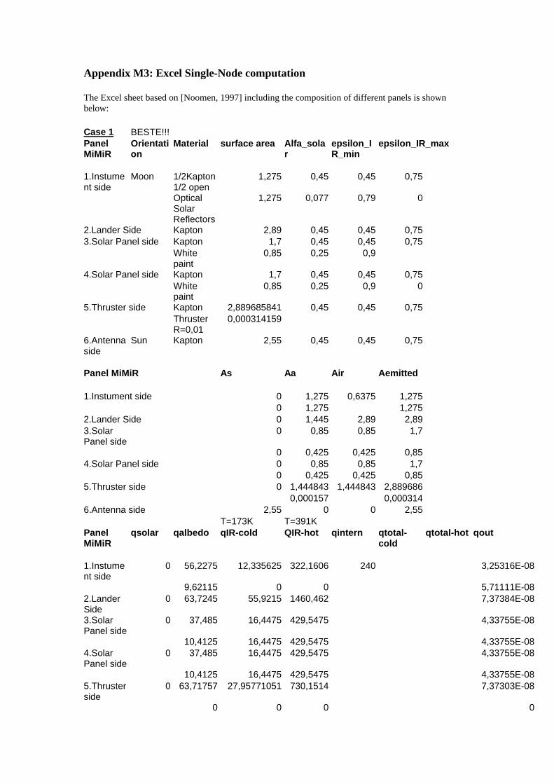
Appendix M3: Excel Single-Node computation The Excel sheet based on [Noomen, 1997] including the composition of different panels is shown below: Case 1 BESTE!!! Panel MiMiR
Orientation
Material surface area Alfa_solar
epsilon_IR_min
epsilon_IR_max
1.Instument side
Moon 1/2Kapton 1/2 open
1,275 0,45 0,45 0,75
Optical Solar Reflectors
1,275 0,077 0,79 0
2.Lander Side Kapton 2,89 0,45 0,45 0,75 3.Solar Panel side Kapton 1,7 0,45 0,45 0,75
White paint
0,85 0,25 0,9
4.Solar Panel side Kapton 1,7 0,45 0,45 0,75 White
paint 0,85 0,25 0,9 0
5.Thruster side Kapton 2,889685841 0,45 0,45 0,75 Thruster
R=0,01 0,000314159
6.Antenna side
Sun Kapton 2,55 0,45 0,45 0,75
Panel MiMiR As Aa Air Aemitted
1.Instument side 0 1,275 0,6375 1,275
0 1,275 1,275 2.Lander Side 0 1,445 2,89 2,89 3.Solar Panel side
0 0,85 0,85 1,7
0 0,425 0,425 0,85 4.Solar Panel side 0 0,85 0,85 1,7
0 0,425 0,425 0,85 5.Thruster side 0 1,444843 1,444843 2,889686
0,000157 0,000314 6.Antenna side 2,55 0 0 2,55
T=173K T=391K Panel MiMiR
qsolar qalbedo qIR-cold QIR-hot qintern qtotal-cold
qtotal-hot qout
1.Instument side
0 56,2275 12,335625 322,1606 240 3,25316E-08
9,62115 0 0 5,71111E-08 2.Lander Side
0 63,7245 55,9215 1460,462 7,37384E-08
3.Solar Panel side
0 37,485 16,4475 429,5475 4,33755E-08
10,4125 16,4475 429,5475 4,33755E-08 4.Solar Panel side
0 37,485 16,4475 429,5475 4,33755E-08
10,4125 16,4475 429,5475 4,33755E-08 5.Thruster side
0 63,71757 27,95771051 730,1514 7,37303E-08
0 0 0 0

6.Antenna side
1606,5 0 0 0 6,50633E-08
1606,5 289,0857 162,0048355 4230,963 240 2297,591 7057,64 4,75677E-07 2212,591 6037,64 50W -600 Steady state T (K)
Radiator Area
1,7 Hot case cold case
Weight 20,4 kg 335,6517 261,1544 1,7 %
Case 2
Panel MiMiR
Orientation
Material surface area Alfa_solar
epsilon_IR_min
epsilon_IR_max
1.Instument side
Moon 1/2Kapton 1/2 open
1,275 0,45 0,45 0,75
Optical Solar Reflectors
1,275 0,077 0,79 0
2.Lander Side Kapton 2,89 0,45 0,45 0,75 3.Solar Panel side Kapton 0 0,45 0,45 0,75
White paint
2,55 0,25 0,9
4.Solar Panel side Kapton 0 0,45 0,45 0,75 White
paint 2,55 0,25 0,9 0
5.Thruster side Kapton 2,889685841 0,45 0,45 0,75 Thruster
R=0,01 0,000314159
6.Antenna side
Sun Kapton 2,55 0,45 0,45 0,75
Panel MiMiR As Aa Air Aemitted
1.Instument side 0 1,275 0,6375 1,275
0 1,275 1,275 2.Lander Side 0 1,445 2,89 2,89 3.Solar Panel side
0 0 0 0
0 1,275 1,275 2,55 4.Solar Panel side 0 0 0 0
0 1,275 1,275 2,55 5.Thruster side 0 1,444843 1,444843 2,889686
0,000157 0,000314 6.Antenna side 2,55 0 0 2,55
Panel MiMiR
qsolar qalbedo qIR-cold QIR-hot qintern qtotal-cold
qtotal-hot qout
1.Instument side
0 56,2275 12,335625 322,1606 240 3,25316E-08
9,62115 0 0 5,71111E-08 2.Lander Side
0 63,7245 55,9215 1460,462 7,37384E-08

3.Solar Panel side
0 0 0 0 0
31,2375 49,3425 1288,643 1,30127E-07 4.Solar Panel side
0 0 0 0 0
31,2375 49,3425 1288,643 1,30127E-07 5.Thruster side
0 63,71757 27,95771051 730,1514 7,37303E-08
0 0 0 0 6.Antenna side
1606,5 0 0 0 6,50633E-08
1606,5 255,7657 194,8998355 5090,058 240 2297,166 7882,99 5,62428E-07 2212,166 6862,99 50W -600 Steady state T (K)
Radiator Area
5,1 Hot case cold case
Weight 61,2 kg 332,3622 250,4308 5,1 %
Case 3
Panel MiMiR
Orientation
Material surface area Alfa_solar
epsilon_IR_min
epsilon_IR_max
1.Instument side
Moon 1/2Kapton 1/2 open
1,275 0,45 0,45 0,75
Optical Solar Reflectors
1,275 0,077 0,79 0
2.Lander Side Kapton 2,89 0,45 0,45 0,75 3.Solar Panel side Kapton 0,85 0,45 0,45 0,75
White paint
1,7 0,25 0,9
4.Solar Panel side Kapton 0,85 0,45 0,45 0,75 White
paint 1,7 0,25 0,9 0
5.Thruster side Kapton 2,889685841 0,45 0,45 0,75 Thruster
R=0,01 0,000314159
6.Antenna side
Sun Kapton 2,55 0,45 0,45 0,75
Panel MiMiR As Aa Air Aemitted
1.Instument side 0 1,275 0,6375 1,275
0 1,275 1,275 2.Lander Side 0 1,445 2,89 2,89 3.Solar Panel side
0 0,425 0,425 0,85
0 0,85 0,85 1,7 4.Solar Panel side 0 0,425 0,425 0,85
0 0,85 0,85 1,7 5.Thruster side 0 1,444843 1,444843 2,889686
0,000157 0,000314 6.Antenna side 2,55 0 0 2,55

Panel MiMiR
qsolar qalbedo qIR-cold QIR-hot qintern qtotal-cold
qtotal-hot qout
1.Instument side
0 56,2275 12,335625 322,1606 240 5,42194E-08
9,62115 0 0 0 2.Lander Side
0 63,7245 55,9215 1460,462 1,22897E-07
3.Solar Panel side
0 18,7425 8,22375 214,7738 3,61463E-08
20,825 32,895 859,095 0 4.Solar Panel side
0 18,7425 8,22375 214,7738 3,61463E-08
20,825 32,895 859,095 0 5.Thruster side
0 63,71757 27,95771051 730,1514 1,22884E-07
0 0 0 0 6.Antenna side
1606,5 0 0 0 1,08439E-07
1606,5 272,4257 178,4523355 4660,511 240 2297,378 7470,315 4,80732E-07 2127,378 5430,315 50W -600 Steady state T (K)
Radiator Area
3,4 Hot case cold case
Weight 40,8 kg 326,0097 257,9203 3,4 %
Case 4
Panel MiMiR
Orientation
Material surface area Alfa_solar
epsilon_IR_min
epsilon_IR_max
1.Instument side
Moon 1/2Kapton 1/2 open
1,275 0,45 0,45 0,75
Optical Solar Reflectors
1,275 0,077 0,79 0
2.Lander Side Kapton 2,89 0,45 0,45 0,75 3.Solar Panel side Kapton 1,275 0,45 0,45 0,75
White paint
1,275 0,25 0,9
4.Solar Panel side Kapton 1,275 0,45 0,45 0,75 White
paint 1,275 0,25 0,9 0
5.Thruster side Kapton 2,889685841 0,45 0,45 0,75 Thruster
R=0,01 0,000314159
6.Antenna side
Sun Kapton 2,55 0,45 0,45 0,75
Panel MiMiR As Aa Air Aemitted
1.Instument side 0 1,275 0,6375 1,275
0 1,275 1,275

2.Lander Side 0 1,445 2,89 2,89 3.Solar Panel side
0 0,6375 0,6375 1,275
0 0,6375 0,6375 1,275 4.Solar Panel side 0 0,6375 0,6375 1,275
0 0,6375 0,6375 1,275 5.Thruster side 0 1,444843 1,444843 2,889686
0,000157 0,000314 6.Antenna side 2,55 0 0 2,55
Panel MiMiR
qsolar qalbedo qIR-cold QIR-hot qintern qtotal-cold
qtotal-hot qout
1.Instument side
0 56,2275 12,335625 322,1606 240 5,42194E-08
9,62115 0 0 0 2.Lander Side
0 63,7245 55,9215 1460,462 1,22897E-07
3.Solar Panel side
0 28,11375 12,335625 322,1606 5,42194E-08
15,61875 24,67125 644,3213 0 4.Solar Panel side
0 28,11375 12,335625 322,1606 5,42194E-08
15,61875 24,67125 644,3213 0 5.Thruster side
0 63,71757 27,95771051 730,1514 1,22884E-07
0 0 0 0 6.Antenna side
1606,5 0 0 0 1,08439E-07
1606,5 280,7557 170,2285855 4445,737 240 2297,484 7263,977 5,16878E-07 2169,984 5733,977 50W -600 Steady state T (K)
Radiator Area
2,55 Hot case cold case
Weight 30,6 kg 324,5391 254,5465 2,55 %
Lander Cornetto surface area
1,53938 surface area
0,513127
qIR qintern Worst case cold 20W/m^2
0,169646 0 0,169646 3,92773E-08 45,588 1,31E-08 59,99718033 0,169646 10 10,16965 3,92773E-08 126,8502 1,31E-08 166,9442215 0,169646 15 15,16965 3,92773E-08 140,1872 1,31E-08 184,4967813 0,169646 20 20,16965 3,92773E-08 150,5356 1,31E-08 198,1159774 0,169646 25 25,16965 3,92773E-08 159,105 1,31E-08 209,3939884 0,169646 35 35,16965 3,92773E-08 172,9843 1,31E-08 227,6601049 0,169646 50 50,16965 3,92773E-08 189,0492 1,31E-08 248,8027587 0,169646 75 75,16965 3,92773E-08 209,1584 1,31E-08 275,267893

APPENIX A: SYSTEMS ENGINEERING DELIVERABLES
APPENDIX A1: WORK BREAKDOWN STRUCTURE APPENDIX A2: WORK PACKAGES APPENDIX A3: PRODUCT TREE APPENDIX A4: WORK BREAKDOWN STRUCTURE APPENDIX A5: REQUIREMENTS DISCOVERY TREE APPENDIX A6: N2 CHART APPENDIX A7: GANTT CHART
APPENDIX B
APPENDIX B1 : NON INTRUSIVE PAYLOAD Neutron spectrometers Gamma ray spectrometers IR spectrometers Microwave spectrometers Miniature Ground Penetrating Radar (Netlander) Radar Altimeter (SSRA, Mars Express) Laser Altimeter (LIDAR, used on Clementine) Raman Spectrometer Optical cameras
APPENDIX B2 : PAYLOAD IN-SITU Gas analysis and Organic Geochemistry Package Evolved Gas Analyser, elemental molecular composition; COSAC Permittivity Probe (PP) Multi-Purpose Sensor for Surface and Subsurface Science (MUPUS) The Mole Rock Grinder and Corer The Robotic arm Mercury Micro-Rover Tunable Diode Laser Sample Acquisition and Transfer Mechanism Cryogenic Drill (SATM) CMOS Active Pixel Sensor Color Camera (APS) CCD Camera
APPENDIX C : LAUNCHERS
APPENDIX D : LAUNCHERS
SOYUZ-FREGAT TSYKLON TAURUS CZ-4 / LM-4
APPENDIX E1 : MASS BREAKDOWN
APPENDIX E2 : VIEW OF THE LANDER
APPENDIX E3 : QBASIC SIMULATION OF THE LANDING PHASE
APPENDIX F
APPENDIX F1 : EULER BUCKLING APPENDIX F2 : SHEAR FLOW OF THE LANDER APPENDIX F3 : LIMIT LOADS OF ADAPTER 937 AT SEPARATION PLANE APPENDIX F4 : MASS MOMENTS OF INERTIA APPENDIX F5 : DRAWINGS OF THE MARS EXPRESS

APPENDIX G
APPENDIX G1: NAVIGATION INSTRUMENTS SPECIFICATION Inertial Measurement Unit Features CCD descent camera Radar Altimeter
APPENDIX G2: KALMAN FILTER APPENDIX G3: RESULTS NAVIGATION SIMULATION APPENDIX G4: MATLAB SOURCE CODE: A CLOSE-LOOP CONTROL-NAVIGATION SENSOR CALIBRATION PROBLEM
APPENDIX H : AOCS
APPENDIX H1: SIMULATION PROGRAM OF THE AOCS OF THE MIMIR ORBITER APPENDIX H2: THE REACTION WHEEL OF THE MIMIR ORBITER APPENDIX H3: SUN SENSOR FOR THE MIMIR ORBITER
Accuracy Field of view Power consumption Electrical output Operating temperature Mass/dimensions Reliability Qualification status Provider
APPENDIX H4: STAR TRACKER APPENDIX H5: SIMULATION PROGRAMME FOR THE MIMIR LANDER 'CORNETTO' APPENDIX H6: SPECIFICATIONS OF THE ATTITUDE CONTROL THRUSTERS OF THE 'CORNETTO' LANDER
APPENDIX I : DELTA-V BUDGET AND ORBIT
APPENDIX I1 : LINK BUDGET APPENDIX I2: THE LTO CALCULATOR
Output graphs Output Data
APPENDIX J : LINK BUDGETS
APPENDIX J1 : LANDER - ORBITER UPLINK BUDGET APPENDIX J2: LANDER – ORBITER DOWNLINK BUDGET APPENDIX J3 : EARTH – ORBITER UPLINK BUDGET APPENDIX J4 : EARTH – ORBITER DOWNLINK BUDGET APPENDIX J5 : DESIGN OPTIONS TREE
APPENDIX K : DETAILS OF THE TEMIC SEMICONDUCTOR TSC21020F PROCESSOR
APPENDIX L : POWER BREAKDOWN STRUCTURES
ORBITER LANDER
APPENDIX M : THERMAL CONTROL
APPENDIX M1: THERMAL CHARACTERISTICS AND FORMULAS APPENDIX M2: MATLAB SINGLE-NODE COMPUTATION APPENDIX M3: EXCEL SINGLE-NODE COMPUTATION