Appendix D Vector Analysis

APPENDIX D. VECTOR ANALYSIS 1

Appendix D

Vector Analysis

The following conventions are used in this appendix and throughout the book:

f, g, φ, ψ are scalar functions of x, t;A,B,C,D are vector functions of x, t;A = |A| ≡

√A ·A is the magnitude or length of the vector A;

eA ≡ A/A is a unit vector in the A direction;x is the vector from the origin to the point (x, y, z);T,W, AB, etc., are dyad (second rank tensor) functions of x, t that will

be called simply tensors;I is the identity tensor or unit dyad;TT is the transpose of tensor T (interchange of indices of the tensor

elements), a tensor;tr(T) is the trace of the tensor T (sum of its diagonal elements), a scalar;det(T) ≡ ‖T‖ is the determinant of the tensor T (determinant of the

matrix of tensor elements), a scalar.

D.1 Vector Algebra

Basic algebraic relations:

A + B = B + A, commutative addition (D.1)A + (B + C) = (A + B) + C, associative addition (D.2)A−B = A + (−B), difference (D.3)fA = Af, commutative scalar multiplication (D.4)(f + g)A = fA + gA, distributive scalar multiplication (D.5)f(A + B) = fA + fB, distributive scalar multiplication (D.6)f(gA) = (fg)A, associative scalar multiplication (D.7)

DRAFT 11:26October 11, 2002 c©J.D Callen, Fundamentals of Plasma Physics


Dot product:

A ·B = 0 implies A = 0 or B = 0, or A ⊥ B (D.8)A ·B = B ·A, commutative dot product (D.9)A · (B + C) = A ·B + A ·C, distributive dot product (D.10)(fA) · (gB) = fg(A ·B), associative scalar, dot product (D.11)

Cross product:

A×B = 0 implies A = 0 or B = 0, or A ‖ B (D.12)A×B = −B×A, A×A = 0, anti-commutative cross product (D.13)A×(B + C) = A×B + A×C, distributive cross product (D.14)(fA)×(gB) = fg(A×B), associative scalar, cross product (D.15)

Scalar relations:

A ·B×C = A×B ·C = (C×A) ·B, dot-cross product (D.16)(A×B) · (C×D) = (A ·C)(B ·D)− (A ·D)(B ·C) (D.17)(A×B) · (C×D) + (B×C) · (A×D) + (C×A) · (B×D) = 0 (D.18)

Vector relations:

A×(B×C) = B(A ·C)−C(A ·B), bac− cab rule= (C×B)×A = A · (CB−BC) (D.19)

A×(B×C) + B×(C×A) + C×(A×B) = 0 (D.20)(A ·B)C = A · (BC), associative dot product (D.21)(A×B)×(C×D) = C(A×B ·D)−D(A×B ·C)

= B(C×D ·A)−A(C×D ·B) (D.22)

Projection of a vector A in directions relative to a vector B:

A = A‖(B/B) + A⊥ = A‖b + A⊥ (D.23)

b ≡ B/B, unit vector in B direction (D.24)A‖ ≡ B ·A/B = b ·A, component of A along B (D.25)

A⊥ ≡ −B×(B×A)/B2, component of A perpendicular to B

= −b×(b×A) (D.26)

D.2 Tensor Algebra

Scalar relations:

I : AB ≡ (I ·A) ·B = A ·B (D.27)AB : CD ≡ A · (B ·C)D = (B ·C)(A ·D)



dotÃproduct crossÃproduct

dot-crossÃproduct

A

B

A

B

A

B

C

{

{ {

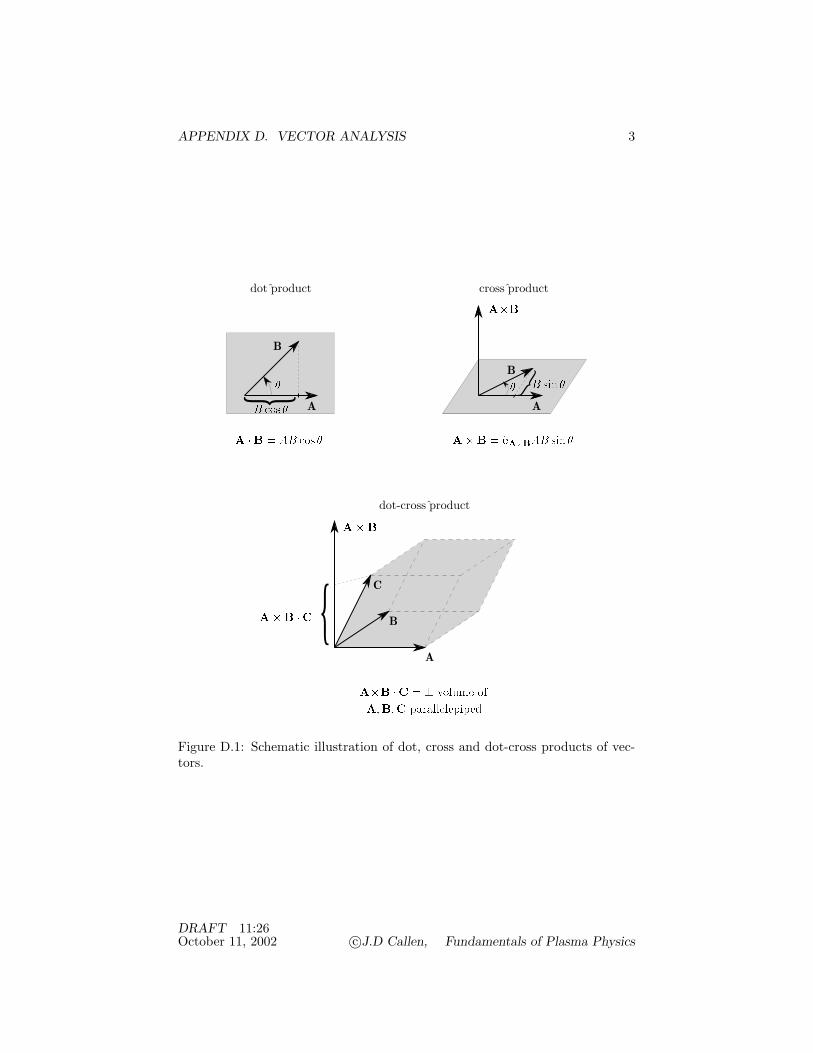
Figure D.1: Schematic illustration of dot, cross and dot-cross products of vec-tors.



= D ·AB ·C = B ·CD ·A (D.28)I : T = tr(T), T : T ≡ |T|2 (D.29)T : AB = (T ·A) ·B = B ·T ·A (D.30)AB : T = A · (B ·T) = B ·T ·A (D.31)B×T : W = −(T ·W)T : B×I (D.32)

Vector relations:

I ·A = A · I = A (D.33)A ·TT = T ·A, TT ·A = A ·T (D.34)A · (CB−BC) = A×(B×C)

= B(A ·C)−C(A ·B), bac− cab rule (D.35)(A×C) ·T = A · (C×T) = −C · (A×T) (D.36)T · (A×C) = (T×A) ·C = −(T×C) ·A (D.37)A · (T×C) = (A ·T)×C = −C×(A ·T) (D.38)(A×T) ·C = A×(T ·C) = −(T ·C)×A (D.39)A · (T×C)−C · (T×A) = [I tr(T)− T] · (A×C) (D.40)(A×T) ·C− (C×T) ·A = (A×C) · [I tr(T)− T] (D.41)

Tensor relations:

I ·AB = (I ·A)B = AB, AB · I = A(B · I) = AB (D.42)I×A = I×A (D.43)A×(BC) = (A×B)C, (AB)×C = A(B×C) (D.44)(A×B)×I = I×(A×B) = BA−AB (D.45)(A×T)T = −TT×A, (T×A)T = −A×TT (D.46)(A×T)− (A×T)T = I×[A tr(T)− T ·A] (D.47)(T×A)− (T×A)T = I×[A tr(T)−A ·T] (D.48)TS = 1

2 (T + TT), symmetric part of tensor T (D.49)TA = 1

2 (T− TT), anti-symmetric part of tensor T (D.50)B×TS×B = B2TS − (BB ·TS + TS ·BB)

− (IB2 −BB)(IB2 −BB) ·TS/B2 −BB(BB ·TS)/B2 (D.51)

D.3 Derivatives

Temporal derivatives:

dAdt

is a vector tangent to the curve defined byA(t) (D.52)

d

dt(fA) =

df

dtA + f

dAdt

(D.53)



d

dt(A + B) =

dAdt

+dBdt

(D.54)

d

dt(A ·B) =

dAdt·B + A · dB

dt(D.55)

d

dt(A×B) =

dAdt×B + A×dB

dt(D.56)

Definitions of partial derivatives in space (∇ ≡ ∂/∂x = del or nabla is thedifferential vector operator):

∇f ≡ ∂f

∂x, gradient of scalar function f , a vector — vector in direction

of and measure of the greatest rate of spatial change of f (D.57)

∇ ·A ≡ ∂

∂x·A, divergence of vector function A, a scalar —

divergence (∇ ·A > 0) or convergence (∇ ·A < 0) of A lines (D.58)

∇×A ≡ ∂

∂x×A, curl (or rotation) of vector function A, a vector1—

vorticity of A lines (D.59)

∇2f ≡∇ ·∇f, del square or Laplacian (divergence of gradient)derivative of scalar function f , a scalar, which is sometimeswritten as ∆f — three-dimensional measure of curvature of f(f is larger where ∇2f < 0 and smaller where ∇2f > 0) (D.60)

∇2A ≡ (∇ ·∇)A =∇(∇ ·A)−∇×(∇×A), Laplacian derivativeof vector function A, a vector (D.61)

For the general vector coordinate x ≡ xex +yey +zez and |x| ≡√x2 + y2 + z2:

∇ · x = 3, ∇ · (x/|x|) = 2/|x| (D.62)∇×x = 0, ∇×(x/|x|) = 0 (D.63)∇|x| = x/|x|, ∇(1/|x|) = −x/|x|3 (D.64)∇x = I (D.65)(A · ∇)(x/|x|) = [A− (x ·A)x/|x|2]/|x| ≡ A⊥/|x| (D.66)∇2(1/|x|) ≡∇ ·∇(1/|x|) = −∇ · (x/|x|3) = −4πδ(x) (D.67)

1Rigorously speaking, the cross product of two vectors and the curl of a vector are pseudo-vectors because they are anti-symmetric contractions of second rank tensors — see tensorreferences at end of this appendix.



First derivatives with scalar functions:

∇(f + g) =∇f +∇g (D.68)∇(fg) = (∇f)g + f∇g =∇(gf) (D.69)∇(fA) = (∇f)A + f∇A (D.70)∇ · fA =∇f ·A + f∇ ·A (D.71)∇×fA =∇f×A + f∇×A (D.72)∇ · fT =∇f ·T + f∇ ·T (D.73)∇×fT =∇f×T + f∇×T (D.74)

First derivative scalar relations:

∇ · (A + B) =∇ ·A +∇ ·B (D.75)∇ · (A×B) = B · ∇×A−A · ∇×B (D.76)(B · ∇)(A ·C) = C · (B · ∇)A + A · (B · ∇)C

≡ CB :∇A + AB :∇C (D.77)A · ∇B ·C−C · ∇B ·A ≡ (CA−AC) :∇B = (A×C) · ∇×B (D.78)2A · ∇B ·C ≡ 2CA :∇B = A · ∇(B ·C) + C · ∇(B ·A)

−B · ∇(A ·C) + (B×C) · (∇×A)+ (B×A) · (∇×C) + (A×C) · (∇×B) (D.79)

I :∇B =∇ ·B (D.80)A×I :∇B = A · ∇×B (D.81)A · ∇ ·T =∇ · (A ·T)−∇A : T =∇ · (A ·T)− T :∇A (D.82)

First derivative vector relations:

∇×(A + B) =∇×A +∇×B (D.83)∇(A ·B) = A×(∇×B) + B×(∇×A) + (A · ∇)B + (B · ∇)A

= (∇A) ·B + (∇B) ·A (D.84)∇(B2/2) ≡∇(B ·B/2) = B×(∇×B) + (B · ∇)B = (∇B) ·B (D.85)(B · ∇)(A×C) = (B · ∇)A×C + A×(B · ∇)C (D.86)∇ ·AB = (∇ ·A)B + (A · ∇)B = (∇ ·A)B + A · (∇B) (D.87)∇ · I = 0 (D.88)∇ · (I×A) =∇×A (D.89)A×(∇×B) = (∇B) ·A−A · (∇B) = (∇B) ·A− (A · ∇)B (D.90)∇×(A×B) = A(∇ ·B)−B(∇ ·A) + (B · ∇)A− (A · ∇)B

=∇ · (BA−AB) (D.91)A · ∇B×C + C×∇B ·A = C×[A×(∇×B)] (D.92)A · ∇B×C−C · ∇B×A = [(∇ ·B)I−∇B] · (A×C) (D.93)A×∇B ·C−C×∇B ·A = (A×C) · [(∇ ·B)I−∇B] (D.94)



First derivative tensor relations:

I · ∇B =∇B, ∇B · I =∇B (D.95)∇×AB = (∇×A)B−A×∇B (D.96)∇(A×B) =∇A×B−∇B×A (D.97)A×∇B +∇B×A

= I×[(∇ ·B)A− (∇B) ·A] + [A · (∇×B)]I−A(∇×B)= I×[(∇ ·B)A−A · (∇B)] + [A · (∇×B)]I− (∇×B)A (D.98)

∇B×A + (A×∇B)T = [A · (∇×B)]I−A(∇×B) (D.99)A×∇B + (∇B×A)T = [A · (∇×B)]I− (∇×B)A (D.100)A×∇B− (A×∇B)T = I×[(∇ ·B)A− (∇B) ·A] (D.101)∇B×A− (∇B×A)T = [(∇ ·B)A−A · (∇B)]×I (D.102)

Second derivative relations:

∇ ·∇f ≡ ∇2f (D.103)∇×∇f = 0 (D.104)∇ ·∇f×∇g = 0 (D.105)∇ ·∇A ≡ ∇2A =∇(∇ ·A)−∇×(∇×A) (D.106)∇ ·∇×A = 0 (D.107)∇ · (B · ∇)A = (B · ∇)(∇ ·A)− (∇×A) · (∇×B) (D.108)∇×[(A · ∇)A]

= (A · ∇)(∇×A) + (∇ ·A)(∇×A)− [(∇×A) · ∇]A (D.109)

Derivatives of projections of A in B direction [b ≡ B/B, A = A‖b + A⊥,A‖ ≡ b ·A, A⊥ ≡ − b×(b×A), (b · ∇)b = − b×(∇×b) ≡ κ]:

∇ ·A = (A‖/B)(∇ ·B) + (B · ∇)(A‖/B) +∇ ·A⊥ (D.110)

∇ ·A⊥ = −A⊥ · [∇ lnB + (b · ∇)b ]− (1/B) b · ∇×(B×A) (D.111)b · ∇A · b ≡ bb :∇A = (b · ∇)A‖ −A⊥ · (b · ∇)b

= A · ∇ lnB − (1/B)b · ∇×(B×A) +∇ ·A− (A‖/B)(∇ ·B) (D.112)

For A⊥ = (1/B2) B×∇f, b · ∇×(B×A⊥) = (b · ∇f)(b · ∇×b) (D.113)

D.4 Integrals

For a volume V enclosed by a closed, continuous surface S with differentialvolume element d3x and differential surface element dS ≡ n dS where n is theunit normal outward from the volume V , for well-behaved functions f, g,A,Band T:∫

V

d3x∇f =∫©∫S

dS f, (D.114)


APPENDIX D. VECTOR ANALYSIS 8∫V

d3x∇ ·A =∫©∫S

dS ·A, divergence or Gauss’ theorem, (D.115)∫V

d3x∇ ·T =∫©∫S

dS ·T, (D.116)∫V

d3x∇×A =∫©∫S

dS×A, (D.117)∫V

d3x f∇2g =∫V

d3x∇f · ∇g +∫©∫S

dS · f∇g,

Green’s first identity, (D.118)∫V

d3x (f∇2g − g∇2f) =∫©∫S

dS · (f∇g − g∇f),

Green’s second identity, (D.119)∫V

d3x [A · ∇×(∇×B)−B · ∇×(∇×A)]

=∫©∫dS · [B×(∇×A)−A×(∇×B)],

vector form of Green’s second identity. (D.120)

The gradient, divergence and curl partial differential operators can be definedusing integral relations in the limit of small surfaces ∆S encompassing smallvolumes ∆V , as follows:

∇f ≡ lim∆V→0

(1

∆V

∫©∫

∆S

dS f)

gradient, (D.121)

∇ ·A ≡ lim∆V→0

(1

∆V

∫©∫

∆S

dS ·A)

divergence, (D.122)

∇×A ≡ lim∆V→0

(1

∆V

∫©∫

∆S

dS×A)

curl. (D.123)

For S representing an open surface bounded by a closed, continuous contour Cwith line element d` which is defined to be positive when the right-hand-rulesense of the line integral around C points in the dS direction:∫∫

S

dS×∇f =∮C

d`f, (D.124)∫∫S

dS · ∇×A =∮C

d` ·A, Stokes’ theorem, (D.125)∫∫S

(dS×∇)×A =∮C

d`×A, (D.126)∫∫S

dS · (∇f×∇g) =∮C

d` · f∇g =∮C

f dg = −∮C

g df,

Green’s theorem. (D.127)

The appropriate differential line element d`, surface area dS, and volume d3xcan be defined in terms of any three differential line elements d`(i), i = 1, 2, 3



that are linearly independent [i.e., d`(1) · d`(2)×d`(3) 6= 0] by

d` = d`(i), i = 1, 2, or 3, differential line element, (D.128)dS = d`(i)×d`(j), differential surface area, (D.129)d3x = d`(1) · d`(2)×d`(3), differential volume. (D.130)

In exploring properties of fluids and plasmas we often want to know howthe differential line, surface and volume elements change as they move with thefluid flow velocity V. In particular, when taking time derivatives of integrals,we need to know what the time derivatives of these differentials are as theyare carried along with a fluid. To determine this, note first that if the flow isuniform then all points in the fluid would be carried along in the same directionat the same rate; hence, the time derivatives of the differentials would vanish.However, if the flow is nonuniform, the differential line elements and hence allthe differentials would change in time. To calculate the time derivatives of thedifferentials, consider the motion of two initially close points x1,x2 as they arecarried along with a fluid flow velocity V(x, t). Using the Taylor series expansionV(x2, t) = V(x1, t)+(x2−x1) · ∇V+· · · and integrating the governing equationdx/dt = V over time, we obtain

x2 − x1 = x2(t = 0)− x1(t = 0) +∫ t

0

dt′ (x′2 − x′1) · ∇V + · · · (D.131)

in which x2(t = 0) and x1(t = 0) are the initial positions at t = 0. Taking thetime derivative of this equation and identifying the differential line element d`as x2−x1 in the limit where the points x2 and x1 become infinetesimally close,we find

d ˙ ≡ d

dt(d`) = d` · ∇V. (D.132)

The time derivative of the differential surface area dS can be calculated bytaking the time derivative of (D.129) and using this last equation to obtain

dS ≡ d

dt(dS) = d ˙ (1)×d`(2) + d`(1)×d ˙ (2)

= d`(1) · ∇V×d`(2)− d`(2) · ∇V×d`(1)= (∇ ·V) dS−∇V · dS (D.133)

in which (D.93) and (D.33) have been used in obtaining the last form. Similarly,the time derivative of the differential volume element moving with the fluid is

d

dt(d3x) = d ˙ (3) · dS + d`(3) · dS

= d`(3) · ∇V · dS + d`(3) · (∇ ·V)dS− d`(3) · ∇V · dS= (∇ ·V) d3x, (D.134)

which shows that the differential volume in a compresssible fluid increases ordecreases according to whether the fluid is rarefying (∇ ·V > 0) or compressing(∇ ·V < 0).



D.5 Vector Field Representations

Any vector field B can be expressed in terms of a scalar potential ΦM and avector potential A:

B = −∇ΦM +∇×A, potential representation. (D.135)

The∇ΦM part of B represents the longitudinal or irrotational (∇×∇ΦM = 0)component while the ∇×A part represents the transverse or solenoidal compo-nent (∇ ·∇×A = 0). A vector field B that satisfies ∇×B = 0 is called a lon-gitudinal or irrotational field; one that satisfies ∇ ·B = 0 is called a solenoidalor transverse field. For a B(x) that vanishes at infinity, the potentials ΦM andA are given by Green’s function solutions

ΦM (x) =∫d3x′

(∇ ·B)x′

4π|x− x′| , A(x) =∫d3x′

(∇×B)x′

4π|x− x′| . (D.136)

When there is symmetry in a coordinate ζ (i.e., a two or less dimensionalsystem), a solenoidal vector field B can be written in terms of a stream functionψ in such a way that it automatically satisfies the solenoidal condition∇ ·B = 0:

B =∇ζ×∇ψ = |∇ζ| eζ×∇ψ = −∇×ψ∇ζ, stream function form.(D.137)

For this situation the vector potential becomes

A = −ψ∇ζ = −ψ |∇ζ| eζ . (D.138)

For a fully three-dimensional situation with no symmetry, a solenoidal vectorfield B can in general be written as

B =∇α×∇β, Clebsch representation, (D.139)

In this representation α and β are stream functions that are constant along thevector field B since B · ∇α = 0 and B · ∇β = 0.

D.6 Properties Of Curve Along A Vector Field

The motion of a point x along a vector field B is described by

dxd`

=BB

= b ≡ T, tangent vector (D.140)

in which d` is a differential distance along B. The unit vector b is tangent tothe vector field B(x) at the point x and so is often written as T — a unit tangentvector.

The curvature vector κ of the vector field B is defined by

κ ≡ d2xd`2

=dbd`

= (b · ∇)b = − b×(∇×b), curvature vector (D.141)



in which (D.85) has been used in the obtaining the last expression. The unitvector in the curvature vector direction is defined by

κ ≡ (b · ∇)b / |(b · ∇)b|, curvature unit vector. (D.142)

The local radius of curvature vector RC is in the opposite direction from thecurvature vector κ and is defined by

RC ≡ −κ/|κ|2, κ = −RC/R2C , radius of curvature. (D.143)

Hence, |RC | ≡ RC = 1/|κ| is the magnitude of the local radius of curvature —the radius of the circle tangent to the vector field B(x) at the point x.

A triad of orthogonal unit vectors (see Fig. D.2) can be constructed from thetangent unit vector T and an arbitrary unit vector N normal (or perpendicular)to the vector field B(x) at the point x:

T ≡ b, N and B ≡ T×N = b×N, Frenet unit vector triad (D.144)

in which B is the binormal unit vector, the third orthogonal unit vector. Thecomponent of a vector C in the direction of the vector field B is called theparallel component: C‖ ≡ T ·C = b ·C. The component in the N direction iscalled the normal component: CN ≡ N ·C. The component in the B direction,which is perpendicular to the T×N plane, is called the binormal component:CB ≡ B ·C = T×N ·C.

Consider for example the components of the curvature vector κ. Sinceb ·κ = 0, the curvature vector has no parallel component (κ‖ = 0) — thecurvature vector for the vector field B(x) is perpendicular to it at the pointx. The components of the curvature vector κ relative to a surface ψ(x) = con-stant in which the vector field lies (i.e., B · ∇ψ = 0) can be specified as follows.Define the normal to be in the direction of the gradient of ψ: N ≡ ∇ψ/|∇ψ|.Then, the components of the curvature vector perpendicular to (normal) andlying within (geodesic) the ψ surface are given by

κn = N ·κ =∇ψ ·κ/|∇ψ|, normal curvature, (D.145)

κg = B ·κ = (b×∇ψ) ·κ/|b×∇ψ|, geodesic curvature. (D.146)

The torsion τ (twisting) of a vector field B is defined by

τ ≡ − dB

d`= − (b · ∇)(b×N), torsion vector. (D.147)

The binormal component of the torsion vector vanishes (τB ≡ B · τ = 0). Thenormal component of the torsion vector locally defines the scale length Lτ alongthe vector B over which the vector field B(x) twists through an angle of oneradian:

Lτ ≡ 1/|τN|, τN ≡ − N · dB

d`= − N · (b · ∇)(b×N), torsion length. (D.148)



B

B

B

curvature torsion

shear

Rc

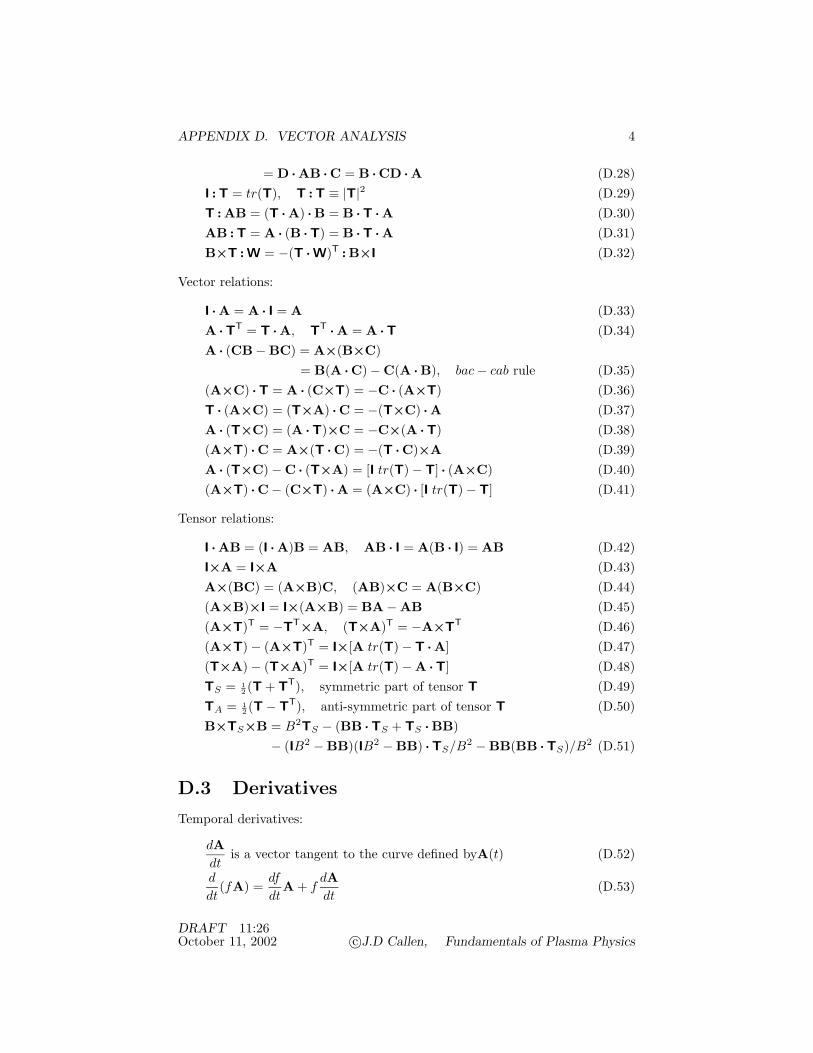
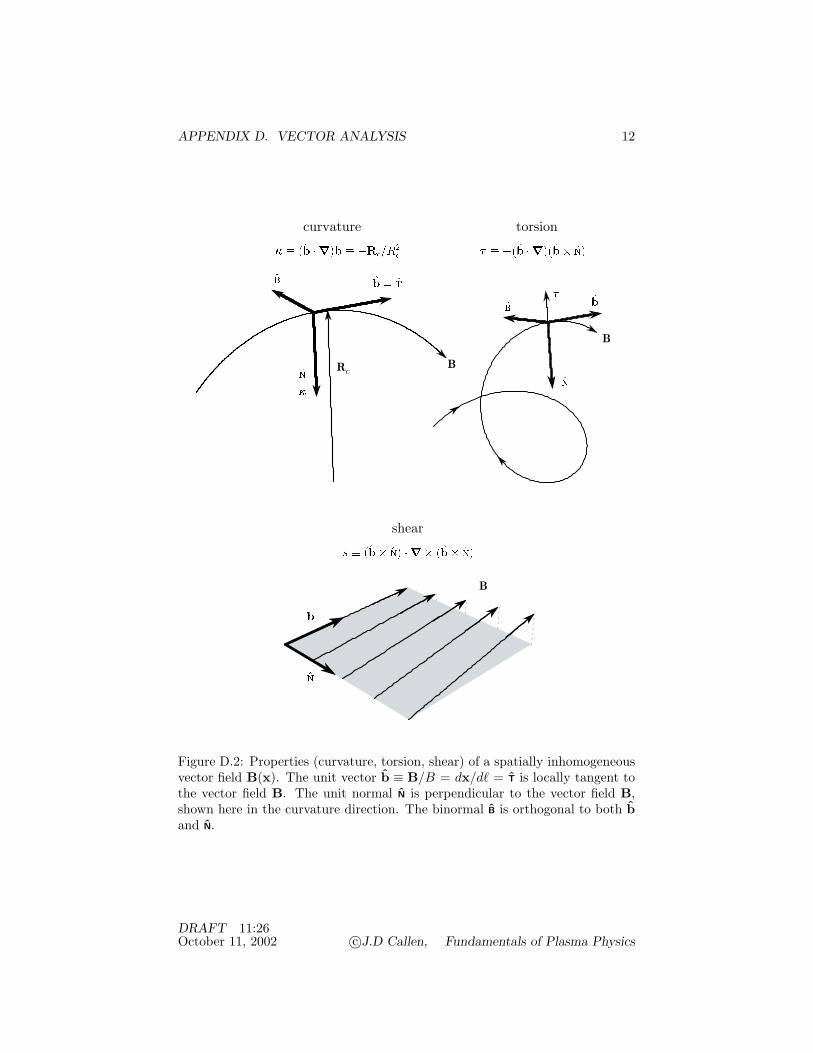
Figure D.2: Properties (curvature, torsion, shear) of a spatially inhomogeneousvector field B(x). The unit vector b ≡ B/B = dx/d` = T is locally tangent tothe vector field B. The unit normal N is perpendicular to the vector field B,shown here in the curvature direction. The binormal B is orthogonal to both band N.



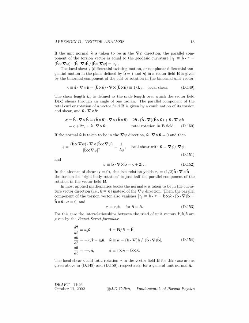
If the unit normal N is taken to be in the ∇ψ direction, the parallel com-ponent of the torsion vector is equal to the geodesic curvature [τ‖ ≡ b · τ =(b×∇ψ) · (b · ∇)b / |b×∇ψ| ≡ κg].

The local shear ς (differential twisting motion, or nonplanar differential tan-gential motion in the plane defined by b = T and N) in a vector field B is givenby the binormal component of the curl or rotation in the binormal unit vector:

ς ≡ B · ∇×B = (b×N) · ∇×(b×N) ≡ 1/LS , local shear. (D.149)

The shear length LS is defined as the scale length over which the vector fieldB(x) shears through an angle of one radian. The parallel component of thetotal curl or rotation of a vector field B is given by a combination of its torsionand shear, and N · ∇×N:

σ ≡ b · ∇×b = (b×N) · ∇×(b×N)− 2N · (b · ∇)(b×N) + N · ∇×N

= ς + 2τN + N · ∇×N, total rotation in B field. (D.150)

If the normal N is taken to be in the ∇ψ direction, N · ∇×N = 0 and then

ς =(b×∇ψ) · ∇×(b×∇ψ)

|b×∇ψ|2≡ 1LS

, local shear with N ≡∇ψ/|∇ψ|,

(D.151)and

σ ≡ b · ∇×b = ς + 2τN. (D.152)

In the absence of shear (ς = 0), this last relation yields τN = (1/2)b · ∇×b —the torsion for “rigid body rotation” is just half the parallel component of therotation in the vector field B.

In most applied mathematics books the normal N is taken to be in the curva-ture vector direction (i.e., N ≡ κ) instead of the∇ψ direction. Then, the parallelcomponent of the torsion vector also vanishes [τ‖ ≡ b · τ = b×κ · (b · ∇)b =b×κ ·κ = 0] and

τ ≡ τNN, for N ≡ κ. (D.153)

For this case the interrelationships between the triad of unit vectors T, N, B aregiven by the Frenet-Serret formulas:

dT

d`= κNN, T ≡ B/B ≡ b,

dN

d`= −κNT + τNB, N ≡ κ = (b · ∇)b / |(b · ∇)b|,

dB

d`= −τNN, B ≡ T×N = b×κ.

(D.154)

The local shear ς and total rotation σ in the vector field B for this case are asgiven above in (D.149) and (D.150), respectively, for a general unit normal N.



D.7 Base Vectors and Vector Components

The three vectors e1, e2, e3, which are not necessarily orthogonal, can be used asa basis for a three-dimensional coordinate system if they are linearly independent(i.e., e1 · e2×e2 6= 0). The three reciprocal base vectors e1, e2, e3 are defined by

ei · ej = δij , (D.155)where

δij ≡{

1, i = j,0, i 6= j,

Kronecker delta. (D.156)

The reciprocal base vectors can be written in terms of the original base vectors:

e1 =e2×e3

e1 · (e2×e3), e2 =

e3×e1

e1 · (e2×e3), e3 =

e1×e2

e1 · (e2×e3). (D.157)

Or, in general index notation

ei = εijkej×ek

e1 · (e2×e3), i, j, k = permutations of 1, 2, 3 (D.158)

in which

εijk =

+1 when i, j, k is an even permutation of 1, 2, 3−1 when i, j, k is an odd permutation of 1, 2, 3

0 when any two indices are equal Levi-Civita symbol.(D.159)

The reciprocal Levi–Civita symbol εijk is the same, i.e., εijk=εijk. These for-mulas are also valid if the subscripts and subscripts are reversed. Thus, the“original” base vectors could be the reciprocal base vectors ei and the “recip-rocal” base vectors could be the original base vectors ei since both sets of basevectors are linearly independent. Either set can be used as a basis for repre-senting three-dimensional vectors.

The identity tensor can be written in terms of the base or reciprocal vectorsas follows:

I ≡∑i eiei = e1e1 + e2e2 + e3e3

≡∑i eie

i = e1e1 + e2e2 + e3e3.identity tensor (D.160)

This definition can be used to write any vector or operator in terms of eitherits base or reciprocal vector components:

A = A · I = (A · e1)e1 + (A · e2)e2 + (A · e3)e3 =∑i

Aiei, Ai ≡ A · ei,

= (A · e1)e1 + (A · e2)e2 + (A · e3)e3 =∑j

Ajej , Aj ≡ A · ej ,

(D.161)∇ ≡ I · ∇ = e1(e1 · ∇) + e2(e2 · ∇) + e3(e3 · ∇)

= e1(e1 · ∇) + e2(e2 · ∇) + e3(e3 · ∇). (D.162)



The dot product between two vectors A and B is given in terms of theirbase and reciprocal vector components by

A ·B =∑i

AiBi =∑i

AiBi =

∑ij

(ei · ej)AiBj =∑ij

(ei · ej)AiBj . (D.163)

Similarly, the cross product between two vectors is given by

A×B =∑ij

AiBj ei×ej =∑ijk

AiBj ek (e1 · e2×e3)

=∑ij

AiBj ei×ej =∑ijk

εijkAiBj ek (e1 · e2×e3)

= (e1 · e2×e3)

∥∥∥∥∥∥e1 e2 e3

A1 A2 A3

B1 B2 B3

∥∥∥∥∥∥ = (e1 · e2×e3)

∥∥∥∥∥∥e1 e2 e3

A1 A2 A3

B1 B2 B3

∥∥∥∥∥∥ . (D.164)

The dot-cross product of three vectors is given by

A ·B×C =∑ijk

AiBjCk ei · ej×ek =∑ijk

εijkAiBjCk (e1 · e2×e3)

=∑ijk

AiBjCk ei · ej×ek =∑ijk

εijkAiBjCk (e1 · e2×e3)

= (e1 · e2×e3)

∥∥∥∥∥∥A1 A2 A3

B1 B2 B3

C1 C2 C3

∥∥∥∥∥∥ = (e1 · e2×e3)

∥∥∥∥∥∥A1 A2 A3

B1 B2 B3

C1 C2 C3

∥∥∥∥∥∥ . (D.165)

For the simplest situation where the three base vectors e1, e2, e3 are orthog-onal (e1 · e2 = e2 · e3 = e1 · e3 = 0), the reciprocal vectors point in the samedirections as the original base vectors. Thus, after normalizing the base andreciprocal vectors they become equal:

e1 = e1/|e1| = e1 = e1/|e1| orthogonale2 = e2/|e2| = e2 = e2/|e2| unite3 = e3/|e3| = e3 = e3/|e3| vectors. (D.166)

The simplifications of (??)–(??) are given in (D.196)–(D.201) in the section(D.9) below on orthogonal coordinate systems.

D.8 Curvilinear Coordinate Systems

Consider transformation from the Cartesian coordinate system x = (x, y, z)to a curvilinear coordinate system labeled by the three independent functionsu1, u2, u3:

x = x(u1, u2, u3) : x = x(u1, u2, u3), y = y(u1, u2, u3), z = z(u1, u2, u3).(D.167)



The transformation is invertible if the partial derivatives ∂x/∂ui for i = 1, 2, 3are continuous and the Jacobian determinant (i.e., ∂x/∂u1 · ∂x/∂u2×∂x/∂u3)formed from these nine partial derivatives does not vanish in the domain ofinterest. The inverse transformation is then given by

ui = ui(x) : u1 = u1(x, y, z), u2 = u2(x, y, z), u3 = u3(x, y, z). (D.168)

In a curvilinear coordinate system there are three coordinate surfaces:

u1(x) = c1 (u2, u3 variable),u2(x) = c2 (u1, u3 variable),u3(x) = c3 (u1, u2 variable).

(D.169)

There are also three coordinate curves given by

u2(x) = c2, u3(x) = c3 (u1 variable),u3(x) = c3, u1(x) = c1 (u2 variable),u1(x) = c1, u2(x) = c2 (u3 variable).

(D.170)

The direction in which ui increases along a coordinate curve is taken to be thepositive direction for ui. If the curvilinear coordinate curves intersect at rightangles (i.e.,∇ui · ∇uj = 0 except for i = j), then the system is orthogonal. Thefamiliar Cartesian, cylindrical and spherical coordinate systems are all orthogo-nal. They are discussed at the end of the next section which covers orthogonalcoordinates.

A nonorthogonal curvilinear coordinate system can be constructed from aninvertible set of functions u1(x), u2(x), u3(x) as follows. A set of base vectorsei can be defined by

ei =∇ui, i = 1, 2, 3 contravariant base vectors. (D.171)

These so-called contravariant (superscript index) base vectors point in the direc-tion of the gradient of the curvilinear coordinates ui, and hence in the directionsperpendicular to the ui(x) = ci surfaces. The set of reciprocal base vectors eiis given by

ei = εijkej×ek

e1 · e2×e3=εijkJ−1∇uj×∇uk, covariant base vectors, (D.172)

in which

J−1 ≡∇u1 · ∇u2×∇u3 = e1 · e2×e3 inverse Jacobian (D.173)

is the Jacobian of the “inverse” transformation from the ui curvilinear coordi-nate system back to the original Cartesian coordinate system.

An alternative form for the reciprocal base vectors can be obtained from thedefinition of the derivative of one of the curvilinear coordinates ui(x) in termsof the gradient: dui = ∇ui · dx = ∇ui ·

∑j(∂x/∂uj) dxj , which becomes an



identity if and only if ∇ui · (∂x/∂uj) = δij . Since this last relation is the sameas the defining relation for reciprocal base vectors (ei · ej = δij), it follows that

ei =∂x∂ui

, i = 1, 2, 3 covariant base vectors. (D.174)

The so-called covariant (subscript index) base vectors point in the directionof the local tangent to the ui variable coordinate curve (from the ∂x/∂ui def-inition), i.e., parallel to the ui coordinate curve. Alternatively, the covariantbase vectors can be thought of as pointing in the direction of the cross productof contravariant base vectors for the two coordinate surfaces other than the ui

coordinate being considered (from the ∇uj×∇uk definition). That these twodirectional definitions coincide follows from the properties of curvilinear sur-faces and curves. The contravariant base vectors ei can also be defined as thereciprocal base vectors of covariant base vectors ei:

ei = εijkej×ek

e1 · e2×e2=εijk

J

∂x∂uj× ∂x∂uk

; i, j, k = permutations of 1, 2, 3

contravariant base vectors(D.175)

in whichJ =

∂x∂u1· ∂x∂u2× ∂x∂u3

= e1 · e2×e3 Jacobian (D.176)

is the Jacobian of the transformation from the Cartesian coordinate system tothe curvilinear coordinate system specified by the functions ui.

The geometrical properties of a nonorthogonal curvilinear coordinate systemare characterized by the dot products of the base vectors:

gij ≡ ei · ej =∂x∂ui· ∂x∂uj

covariant metric elements,

gij ≡ ei · ej =∇ui · ∇uj contravariant metric elements.(D.177)

These symmetric tensor metric elements can be used to write the covariantcomponents of a vector in terms of its contravariant components and vice versa:

Ai ≡ A · ei = A · I · ei =∑j

(A · ej)(ej · ei) =∑j

gij Aj

Ai ≡ A · ei = A · I · ei =∑j

(A · ej)(ej · ei) =∑j

gijAi.(D.178)

Similarly, they can also be used to write the covariant base vectors in terms ofthe contravariant base vectors and vice versa:

ei =∑j

gij ej , ei =∑j

gij ei. (D.179)

From the dot product between these relations and their respective reciprocalbase vectors it can be shown that∑

j

gij gjk =

∑j

gkjgji = δki . (D.180)



The determinant of the matrix comprised of the metric coefficients is calledg:

g ≡ ‖gij‖ =∥∥gij∥∥−1

, (D.181)

in which the second relation follows from interpreting the summation relationsat the end of the preceding paragraph in terms of matrix operations: [gij ][gik]= [I], which yields [gij ] = [gjk]−1. Since the determinant of the inner productof two matrices is given by the product of the determinants of the two matrices,

g = ‖gij‖ =∥∥∥∥ ∂x∂ui· ∂x∂uj

∥∥∥∥ =∥∥∥∥ ∂x∂ui

∥∥∥∥∥∥∥∥ ∂x∂uj

∥∥∥∥ =(∂x∂u1· ∂x∂u2× ∂x∂u3

)2

= J2.

(D.182)Thus, the determinant of the metric coefficients is related to the Jacobian andinverse Jacobian as follows:

J =√g = e1 · e2×e3 =

∂x∂u1· ∂x∂u2× ∂x∂u3

Jacobian,

J−1 = 1/√g = e1 · e2×e3 =∇u1 · ∇u2×∇u3 inverse Jacobian.

(D.183)

The various partial derivatives in space can be worked out in terms of covari-ant derivatives (∂/∂ui) using the properties of the covariant and contravariantbase vectors for a general, nonorthogonal curvilinear coordinate system as fol-lows:

∇f =∑i

∇ui ∂f∂ui

=∑i

ei∂f

∂uigradient,

(D.184)

∇ ·A = ∇ · (A · I) =∇ ·∑i

√g (A · ei) ei√

g=∑i

ei√g· ∇(√gAi)

=∑i

1√g

∂

∂ui(√gA · ei) =

∑i

1J

∂

∂ui(J A · ∇ui) divergence,

(D.185)∇×A =∇×(A · I) =∇×

∑j

(A · ej)ej =∑j

∇Aj×∇uj

=∑ij

∂Aj∂ui∇ui×∇uj =

∑ijk

εijk√g

∂(A · ej)∂ui

=1√g

∥∥∥∥∥∥e1 e2 e3∂∂u1

∂∂u2

∂∂u3

A1 A2 A3

∥∥∥∥∥∥ curl,

(D.186)



∇2f ≡∇ ·∇f =∑i

1√g

∂

∂ui(√g ei ·

∑j

ej∂f

∂uj)

=∑ij

1√g

∂

∂ui(√g gij

∂f

∂uj) =

∑ij

1J

∂

∂ui(J∇ui · ∇uj ∂f

∂uj) Laplacian.

(D.187)Differential line, surface and volume elements can be written in terms of

differentials of the coordinates ui of a general, nonorthogonal curvilinear coor-dinate system as follows. Total vector differential and line elements are:

dx =∑i

∂x∂ui

dxi =∑i

ei dxi

|d`| ≡√dx · dx =

√∑ij gij du

iduj metric of coordinates.(D.188)

Differential line elements d`(i) along curve ui (duj = duk = 0) for i, j, k =permutations of 1, 2, 3 are

d`(i) = ei dui =εijk√g∇uj×∇uk dui

|d`(i)| = √ei · ei dui =√gii du

i

(D.189)

The differential surface element dS(i) in the ui = ci surface (dui = 0) for i, j, k= permutations of 1, 2, 3 is

dS(i) ≡ d`(j)×d`(k) =√g εijk∇ui dujduk

|dS(i)| =√gjjgkk − g2

jk dujduk =

√giig dujduk

(D.190)

The differential volume element is

d3x ≡ d`(1) · d`(2)×d`(3) = e1 · (e2×e3) du1du2du3 =√g du1du2du3.

(D.191)

D.9 Orthogonal Coordinate Systems

Consider transformation from the Cartesian coordinate system x = (x, y, z)to an orthogonal curvilinear coordinate system defined by three independentfunctions ui = ui(x, y, z) for i = 1, 2, 3. [Here, the superscripts 1,2,3 are notpowers; rather, they represent labels for the three functions. The functions arelabeled in this way to maintain consistency with the general (nonorthogonal)curvilinear coordinate literature.] The coordinate surfaces are defined by ui =ci, where ci are constants. The three orthogonal unit vectors that point indirections locally perpendicular to the coordinate surfaces are

ei ≡∇ui/|∇ui| orthogonal unit vectors. (D.192)



For the simplest orthogonal coordinate system, the Cartesian coordinate system,e1 =∇x = x, e2 =∇y = y, e3 =∇z = z.

Because of the normalization and assumed orthogonality of these unit vec-tors,

ei · ej = δij ≡{

1, for i = j,0, for i 6= j,

Kronecker delta. (D.193)

The cross products of unit vectors are governed by the right-hand rule which isembodied in the mathematical relation

ei×ej = εijk ek (D.194)

in which the Levi-Civita symbol εijk is defined by

εijk ≡

+1, for i, j, k = 1, 2, 3 or 2, 3, 1 or 3, 1, 2 (even permutations)−1, for i, j, k = 2, 1, 3 or 1, 3, 2 or 3, 2, 1 (odd permutations)

0, for any two indices the same.(D.195)

A vector A can be represented in terms of its components in the orthogonaldirections (parallel to ∇ui) of the unit vectors ei:

A =∑i

Aiei = A1e1 +A2e2 +A3e3, Ai ≡ A · ei (D.196)

For an orthogonal coordinate system the identity dyad or tensor is

I =∑i

eiei = e1e1 + e2e2 + e3e3 identity tensor. (D.197)

Thus, the vector differential operator becomes

∇ = I · ∇ =∑i

ei (ei · ∇) = e1 (e1 · ∇) + e2 (e2 · ∇) + e3 (e3 · ∇)

=∑i

∇ui ∂∂ui

=∇u1 ∂

∂u1+∇u2 ∂

∂u2+∇u3 ∂

∂u3.

(D.198)

Here and below the sum over i is over the three components 1,2,3.Using the relations for the dot and cross products of the unit vectors ei given

in (D.193) and (D.194) the dot, cross and dot-cross products of vectors become

A ·B =∑i

AiBi = A1B1 +A2B2 +A3B3, (D.199)

A×B =∑ij

AiBj ei×ej =∑ijk

εijk AiBj ek =

∥∥∥∥∥∥e1 e2 e3

A1 A2 A3

B1 B2 B3

∥∥∥∥∥∥= e1(A2B3 −A3B2) + e2(A3B1 −A1B2) + e3(A1B2 −A2B1). (D.200)

A ·B×C =∑ijk

εijk AiBjCk =

∥∥∥∥∥∥A1 A2 A3

B1 B2 B3

C1 C2 C3

∥∥∥∥∥∥ . (D.201)



The differential line element in the ith direction is given by

d`(i) = ei hi dui, with hi ≡ 1/|∇ui|, differential line element. (D.202)

Thus, the differential surface vector for the ui = ci surface, which is defined bydS(i) = d`(j)×d`(k), becomes

dS(i) = ei hjhk dujduk, for i 6= j 6= k, differential surface area. (D.203)

Since the differential volume element is d3x = d`(i) · dS(i) = d`(1) · d`(2)×d`(3)and the Jacobian of the transformation is given by J = 1/(∇u1 · ∇u2×∇u3)= h1h2h3,

d3x = h1h2h3 du1du2du3, differential volume. (D.204)

For orthogonal coordinate systems the various partial derivatives in spaceare

∇f =∑i

eihi

∂f

∂ui=∑i

ei (ei · ∇) f, (D.205)

∇ ·A =∑i

1J

∂

∂ui

(J

hiA · ei

)=∑i

1h1h2h3

∂

∂ui

(h1h2h3

hiA · ei

), (D.206)

∇×A =∑ijk

εijkhkekJ

∂

∂ui(hjA · ej) =

∑ijk

εijkhkekh1h2h3

∂

∂ui(hjA · ej), (D.207)

∇2f =∑i

1J

∂

∂ui

(J

h2i

∂f

∂ui

)=∑i

1h1h2h3

∂

∂ui

(h1h2h3

h2i

∂f

∂ui

). (D.208)

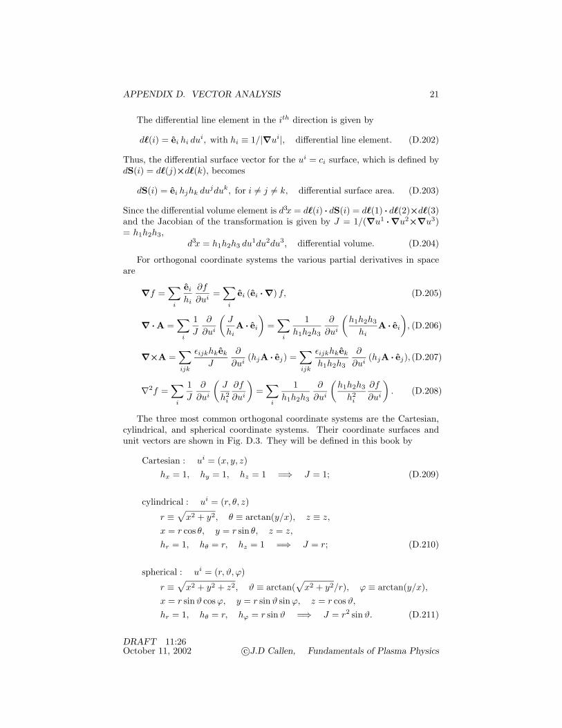
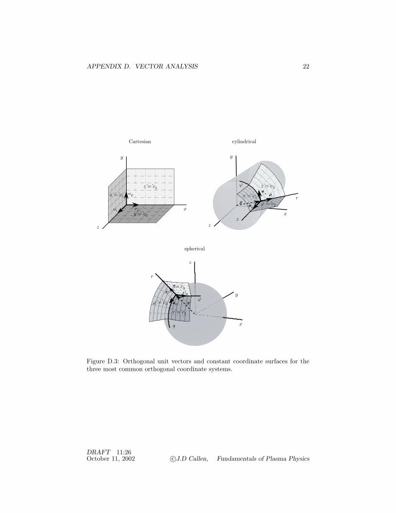
The three most common orthogonal coordinate systems are the Cartesian,cylindrical, and spherical coordinate systems. Their coordinate surfaces andunit vectors are shown in Fig. D.3. They will be defined in this book by

Cartesian : ui = (x, y, z)hx = 1, hy = 1, hz = 1 =⇒ J = 1; (D.209)

cylindrical : ui = (r, θ, z)

r ≡√x2 + y2, θ ≡ arctan(y/x), z ≡ z,

x = r cos θ, y = r sin θ, z = z,

hr = 1, hθ = r, hz = 1 =⇒ J = r; (D.210)

spherical : ui = (r, ϑ, ϕ)

r ≡√x2 + y2 + z2, ϑ ≡ arctan(

√x2 + y2/r), ϕ ≡ arctan(y/x),

x = r sinϑ cosϕ, y = r sinϑ sinϕ, z = r cosϑ,hr = 1, hθ = r, hϕ = r sinϑ =⇒ J = r2 sinϑ. (D.211)



x

y

z

r

ϕ

xÃ=Ãc1

yÃ=Ãc2

zÃ=Ãc3

rÃ=Ãc1

ϕÃ=Ãc2

zÃ=Ãc3

rÃ=Ãc1

ϕÃ=Ãc3

x

x

y

z

x

y

z

x

r

ϕ

z

Cartesian cylindrical

spherical

Ã=Ãc

Figure D.3: Orthogonal unit vectors and constant coordinate surfaces for thethree most common orthogonal coordinate systems.



Note that with these definitions the cylindrical angle θ is the same as the az-imuthal (longitudinal) spherical angle ϕ, but that the radial coordinate r isdifferent in the cylindrical and spherical coordinate systems. The spherical an-gle ϑ is a latitude angle — see Fig. D.3. Explicit forms for the various partialderivatives in space, (D.205) – (D.208), are given in Appendix Z.

REFERENCES

Intermediate level discussions of vector analysis are provided in

Greenberg, Advanced Engineering Mathematics, Chapters 13-16 (1998) [?]

Kusse and Westwig, Mathematical Physics (1998) [?]

Danielson, Vectors and Tensors in Engineering and Physics, 2nd Ed. (1997) [?]

More advanced treatments are available in

Arfken, Mathematical Methods for Physicists (??) [?]

Greenberg, Foundations of Applied Mathematics, Chapters 8,9 (1978) [?]

Morse and Feshbach, Methods of Theoretical Physics, Part I, Chapter 1 (1953)[?]


Documents

Appendix D Vector Analysis