Appendix I Elements of Fluid Mechanics

The analysis of groundwater flow requires an understanding of the elements of fluid mechanics. Albertson and Simons (1964) provide a useful short review; Streeter (1962) and Yennard (1961) are standard texts. Our purpose here is simply to introduce the basic fluid properties: mass density, weight density, compressibility, and viscosity; and to examine the concepts of fluid pressure and pressure head.

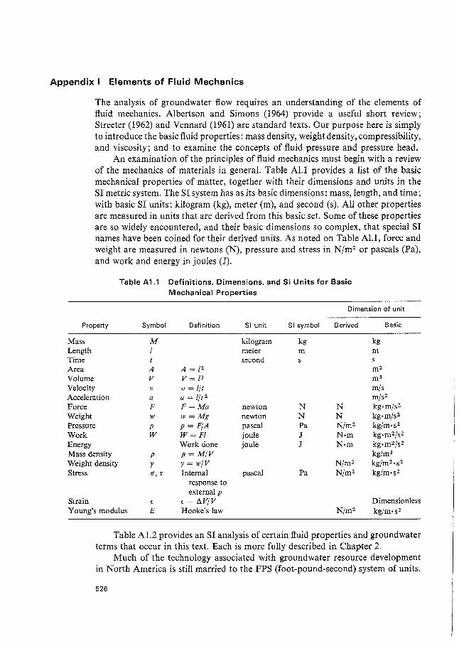
An examination of the principles of fluid mechanics must begin with a review of the mechanics of materials in general. Table Al. I provides a list of the basic mechanical properties of matter, together with their dimensions and units in the SI metric system. The SI system has as its basic dimensions: mass, length, and time; with basic SI units: kilogram (kg), meter (m), and $econd (s). All other properties are measured in units that are derived from this basic set. Some of these properties are so widely encountered, and their basic dimensions so complex, that special SI names have been coined for their derived units. As noted on Table Al. I, force and weight are measured in newtons (N), pressure and stress in N/m2 or pascals (Pa), and work and energy in joules (J).

Table A1 .1 Definitions, Dimensions, and SI Units for Basic Mechanical Properties

Dimension of unit

Property Symbol Definition SI unit SI symbol Derived Basic

Mass M kilogram kg kg Length I meter m m Time t second s Area A A= 12 m2 Volume v V= /3 m3 Velocity v v =!ft m/s Acceleration a a= l/t2 m/s2

Force F F=Ma newton N N kg•m/s2

Weight w w=Mg newton N N kg·m/s2 Pressure p p =F/A pascal Pa N/m2 kg/m•s2 Work w W=Ff joule J N·m kg·m2/s2 Energy Work done joule J N·m kg·m2/s2

Mass density p p=M/V kg/m3 Weight density y y = w/V N/m3 kg/m2·s2 Stress O', 't' Internal pascal Pa N/m2 kg/m•s2

response to external p

Strain f £ = 11V/V Dimensionless Young's modulus E Hooke's law N/m2 kg/m•s2

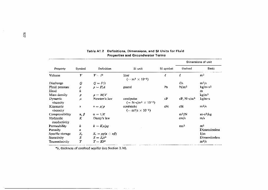
Table A 1.2 provides an SI analysis of certain fluid properties and groundwater terms that occur in this text. Each is more fully described in Chapter 2.

Much of the technology associated with groundwater resource development in North America is still married to the FPS (foot-pound-second) system of units.

526

01 I\)

"

Property Symbol

Volume v

Discharge Q Fluid pressure p Head h Mass density p Dynamic µ

viscosity Kinematic v

viscosity Compressibility fX, p Hydraulic K

conductivity Permeability k Porosity n Specific storage Ss Storativity s Transmissivity T

Table A1 .2 Definitions, Dimensions, and SI Units for Fluid Properties and Groundwater Terms

Dimensions of unit

Definition SI unit SI symbol Derived Basic

V= /3 liter t t m3 (= m3 x lQ-3)

Q = /3/t t/s m3/s p =FIA pascal Pa N/m2 kg/m·s2

m p=M/V kg/m3 Newton's law centipoise cP cP, N·s/m2 kg/m•s

( = N ·s/m2 x 10-3) v = µ/p centistoke cSt cSt m2/s

( = m2/s x 10-6) 1" = 1/E m2/N m•s2/kg Darcy's law emfs m/s

k = Kµ/pg cm2 m2 Dimensionless

Ss = pg((f, + nP) 1/m S = Ssb* Dimensionless T=Kb* m2/s

*b, thickness of confined aquifer (see Section 2.10).

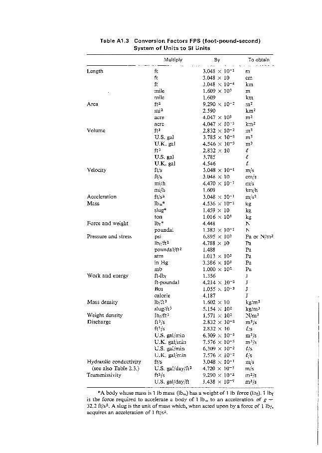
Table A1.3 Conversion Factors FPS (foot-pound-second) System of Units to SI Units

Multiply By To obtain

Length ft 3.048 x 10-1 m ft 3.048 x 10 cm ft 3.048 x 10-4 km mile 1.609 x 103 m mile 1.609 km

Area ft 2 9.290 x 10-2 m2 mi 2 2.590 km2

acre 4.047 x 103 m2 acre 4.047 x 10-3 km2

Volume ft 3 2.832 x 10-2 m3 U.S. gal 3.785 x 10-3 m3 U.K. gal 4.546 x 10-3 m3 ft3 2.832 x 10 (

U.S. gal 3.785 t U.K. gal 4.546 (

Velocity ft/s 3.048 x 10-1 m/s ft/s 3.048 x 10 cm/s mi/h 4.470 x 10-1 m/s mi/h 1.609 km/h

Acceleration ft/s 2 3.048 x 10-1 m/s2

Mass lbm* 4.536 x 10-1 kg slug* 1.459 x 10 kg ton 1.016 x 103 kg

Force and weight lbr* 4.448 N poundal 1.383 x 10-1 N

Pressure and stress psi 6.895 x 103 Pa or N/m2 lbr/ft2 4.788 x 10 Pa poundal/ft2 1.488 Pa atm 1.013 x 10s Pa in Hg 3.386 x 103 Pa mb 1.000 x 102 Pa

Work and energy ft-lbr 1.356 J ft-poundal 4.214 x 10-2 J Btu 1.055 x 10-3 J calorie 4.187 J

Mass density lb/ft3 1.602 x 10 kg/m3 slug/ft3 5.154 x 102 kg/m3

Weight density lbr/ft3 1.571 x 102 N/m3 Discharge ft 3 /s 2.832 x 10-2 m3/s

ft,3/s 2.832 x 10 (js U.S. gal/min 6.309 x 10-s m3/s U.K. gal/min 7.576 x 10-s m3/s U.S. gal/min 6.309 x 10-2 (js U .K. gal/min 7.576 x 10-2 (js

Hydraulic conductivity ft/s 3.048 x 10-1 m/s (see also Table 2.3.) U.S. gal/day/ft2 4.720 x 10-1 m/s

Transmissivity ft 2/s 9.290 x 10-2 m2/s U.S. gal/day/ft 1.438 x 10-1 m2/s

*A body whose mass is 1 lb mass (lbm) has a weight of 1 lb force (lbr). 1 lbr is the force required to accelerate a body of 1 lbm to an acceleration of g =

32.2 ft/s 2. A slug is the unit of mass which, when acted upon by a force of 1 lbr, acquires an acceleration of 1 ft/s 2.

529 Appendix I

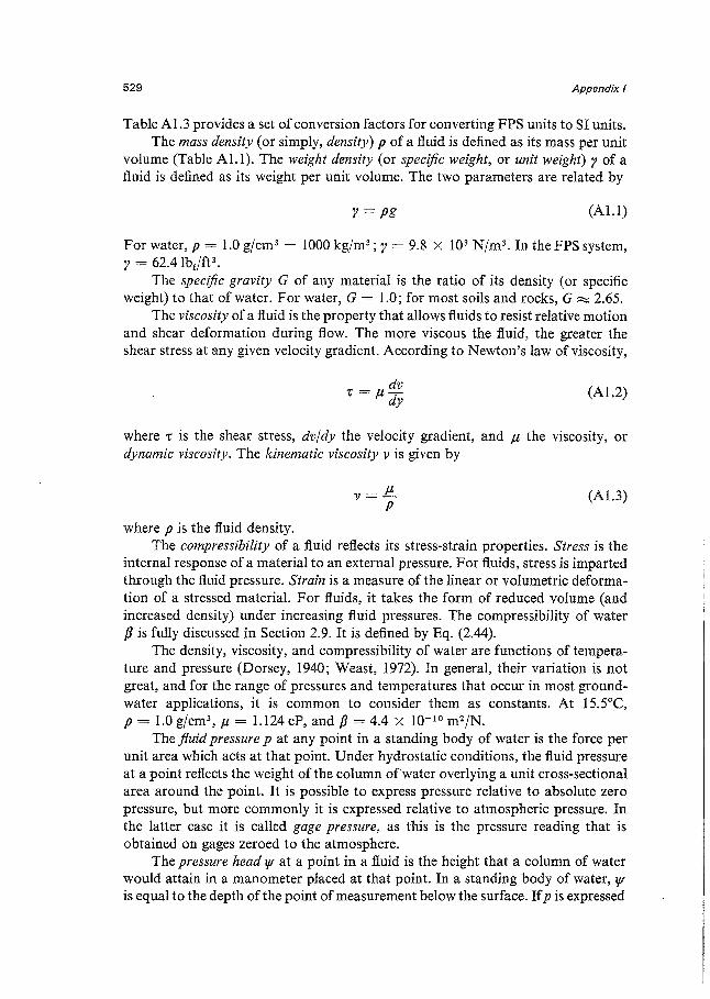
Table Al .3 provides a set of conversion factors for converting FPS units to SI units. The mass density (or simply, density) p of a fluid is defined as its mass per unit

volume (Table Al. I). The weight density (or specific weight, or unit weight) y of a fluid is defined as its weight per unit volume. The two parameters are related by

y =pg (Al.I)

For water, p = 1.0 g/cm3 = 1000 kg/m3 ; y = 9.8 x 103 N/m3 • In the FPS system, y = 62.4 lbr/ft 3

•

The specific gravity G of any material is the ratio of its density (or specific weight) to that of water. For water, G = 1.0; for most soils and rocks, G ~ 2.6S.

The viscosity of a fluid is the property that allows fluids to resist relative motion and shear deformation during flow. The more viscous the fluid, the greater the shear stress at any given velocity gradient. According to Newton's law of viscosity,

dv 7: = µ­

dy (AI.2)

where 7: is the shear stress, dv/dy the velocity gradient, and µ the viscosity, or dynamic viscosity. The kinematic viscosity vis given by

where pis the fluid density.

v = !!:_ p

(Al.3)

The compressibility of a fluid reflects its stress-strain properties. Stress is the internal response of a material to an external pressure. For fluids, stress is imparted through the fluid pressure. Strain is a measure of the linear or volumetric deforma­tion of a stressed material. For fluids, it takes the form of reduced volume (and increased density) under increasing fluid pressures. The compressibility of water pis fully discussed in Section 2.9. It is defined by Eq. (2.44).

The density, viscosity, and compressibility of water are functions of tempera­ture and pressure (Dorsey, 1940; Weast, 1972). In general, their variation is not great, and for the range of pressures and temperatures that occur in most ground­water applications, it is common to consider them as constants. At IS.S°C, p = 1.0 g/cm3 , µ = 1.124 cP, and p = 4.4 x 10- 10 m2/N.

The fluid pressure p at any point in a standing body of water is the force per unit area which acts at that point. Under hydrostatic conditions, the fluid pressure at a point reflects the weight of the column of water overlying a unit cross-sectional area around the point. It is possible to express pressure relative to absolute zero pressure, but more commonly it is expressed relative to atmospheric pressure. In the latter case it is called gage pressure, as this is the pressure reading that is obtained on gages zeroed to the atmosphere.

The pressure head l/f at a point in a fluid is the height that a column of water would attain in a manometer placed at that point. In a standing body of water, l/f is equal to the depth of the point of measurement below the surface. If pis expressed

530 Appendix I

as a gage pressure, VI is defined by the relationship

P = pgVI = YVI (Al.4)

In effect, the pressure head VI is a measurement of the fluid pressure p. Fluid pressures are also developed in groundwater as it flows through porous

geological formations and soils. In Section 2.2, the elements of fluid mechanics presented in this appendix are applied in the development of groundwater flow theory.

Appendix II Equation of Flow for Transient Flow Through Deforming Saturated Media

A rigorous development of the equation of flow for transient flow in saturated media must recognize the fact that transient changes in fluid pressure lead to deformations in the granular skeleton of a porous medium, and these deformations imply that the medium, as well as the water, is in motion. This realization creates the need for two refinements to the classical derivation presented by Jacob (1940) and followed in Section 2.11 of this text. First, as recognized by Biot (1955), it is necessary to cast Darcy's law in terms of the relative velocity of fluid to grains. And second, as recognized by Cooper (1966), it is necessary to consider the con­servation of mass for the medium as well as for the fluid in the elemental control volume. One can develop the continuity relationships in one of three ways: (1) by considering a deforming elemental volume in deforming coordinates, (2) by con­sidering a deforming elemental volume in fixed coordinates, or (3) by considering a fixed elemental volume in fixed coordinates. Following Gambolati and Freeze (1973), we will use a fixed elemental volume in fixed coordinates. The approach requires the use of vector notation and the material derivative (total derivative, substantial derivative). If these concepts are not familiar, Aris (1962) and Wills (1958) provide introductory treatments. The development will be presented here for a homogeneous, isotropic medium with hydraulic conductivity K, porosity n, and vertical compressibility (!,. The same approach is easily adapted to heterogene­ous and anisotropic media.

In vector notation, the three-dimensional form of Darcy's law [Eq. (2.34)] is

~ = -KVh (A2.l)

where ~ = (vx, Vy, vz) is the relative velocity of fluid to grains, and Vh = (ah/ax, ah/ay, ah/az) is the hydraulic gradient. We can expand the vector ~ as

(A2.2)

where ~w is the fluid velocity and ~ s the velocity of the deforming medium. The equation of state for the water [Eq. (2.47)] is

(A2.3)

and that for the soil grains, which are incompressible, is

Ps =.constant (A2.4)

The equation of continuity for the water is

(A2.5)

531

532 Appendix If

and that for the soil is

(A2.6)

In these equations V . is the divergence operator:

a a a V-=-+-+-ax ay az Expanding Eq. (A2.5), we arrive at

_,. _,. ap an -pV · (nvw) - nvw • V p = n di + p at (A2.7)

If we cancel Ps from Eq. (A2.6) and rearrange that equation, we obtain an expres­sion for an;at. This can be substituted in Eq. (A2.7) together with an expression for nvw obtained from Eq. (A2.2). After dividing through by p and rearranging, Eq. (A2.7) becomes

-V • V - (~) · Vp = (;)(~ + V, • Vp) + V • V, (A2.8)

Ifwe use the material derivative, D/Dt = a;at +vs· V, Eq. (A2.8) can be written as

-V · v - ( v) · V p = !!:_ Dp + V · v p p Dt s (A2.9)

The first term on the right-hand side of Eq. (A2.9) can be related to the compress­ibility of water p by the relation

Dp =pp DP Dt Dt

(A2.IO)

The material derivative on the right-hand side of Eq. (A2.IO) can be replaced by a partial derivative only if the following inequality is satisfied:

(A2.ll)

Let us further assume, on the left-hand side of Eq. (A2.9), that

(~)·Vp~V·v (A2.12)

Then, substituting Eqs. (A2.l) and (A2.IO) in Eq. (A2.9) yields

ap ..,. V • (K Vh) = nP at + V • vs (A2.13)

533 Appendix II

In a three-dimensional stress field, the grain velocity vector vs = ( v sx' v sy' v sz) is related to the deformation (or soil displacement) vector~ = (ux, uy, uz) by

D~ Vs= Dt (A2.14)

In a one-dimensional vertical stress field,

(A2.15)

If the conditions of Eq. (A2.15) are satisfied, the final term of Eq. (A2.13) can be expanded (Cooper, 1966; Gambolati and Freeze, 1973; Gambolati, 1973a) as

v . v = avsz = j_(Duz) = R(iluz) = (/, Dp s ilz ilz Dt Dt ilz Dt

(A2.16)

where t;t is the vertical compressibility of the porous medium. The change of derivative around the central equality is valid for a position vector but not in general. The material derivative in the right-hand expression of Eq. (A2.16) can be replaced by the partial derivative if Eq. (A2.11) is satisfied. In that case, Eq. (A2.13) becomes

Since p = pg(h - z) and K is a constant, Eq. (A2. l 7) simplifies to

vzh = pg(t;t + nP) ilh K ilt

Or, recalling that Ss = pg(rx + np) and expanding the vector notation,

il2h il2h il2h s ilh axz + i)y2 + i)z2 = K Jt

(A2.l 7)

(A2.18)

(A2.19)

Equation (A2.19) is identical to Eq. (2.75) developed by Jacob (1940). The more rigorous development makes it clear that the validity of the classical equation of flow rests on the satisfaction of the inequalities of Eqs. (A2.11) and (A2.12) and the stress condition of Eq. (A2. l 5). It is unlikely that these conditions are always satisfied. Gambolati (I 973b) shows that where the rate of consolidation vs exceeds the rate of percolating fluid vw, as it can in thick clay layers oflow permeability and high compressibility, the inequalities may not be satisfied. With regard to the stress condition, the V • vs term at the end of Eq. (A2.13) is really the protruding tip of an iceberg that relates the three-dimensional flow field to the three-dimensional stress field. Biot (1941, 1955) first exposed the interrelationships and Verruijt (1969) provides a clear derivation. Schiffman et al. (1969) provides a comparison of the classical and Biot approaches, and Gambolati (1974) analyses the range of validity of the classical equation of flow.

Appendix Ill Example of an Analytical Solution to a Boundary-Value Problem

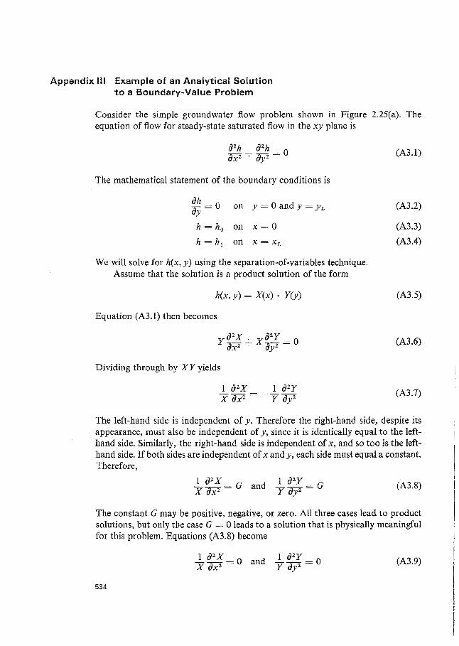
Consider the simple groundwater flow problem shown in Figure 2.25(a). The equation of flow for steady-state saturated flow in the xy plane is

(A3.l)

The mathematical statement of the boundary conditions is

ah_ 0 ay- on y = 0 and y = YL (A3.2)

h = h0 on x=O (A3.3)

h =hi on X =XL (A3.4)

We will solve for h(x, y) using the separation-of-variables technique. Assume that the solution is a product solution of the form

h(x, y) = X(x) · Y(y) (A3.5)

Equation (A3.1) then becomes

(A3.6)

Dividing through by XY yields

(A3.7)

The left-hand side is independent of y. Therefore the right-hand side, despite its appearance, must also be independent of y, since it is identically equal to the left­hand side. Similarly, the right-hand side is independent of x, and so too is the left­hand side. If both sides are independent of x and y, each side must equal a constant. Therefore,

1 azx 1 azy X ax2 = G and y ay2 = G (A3.8)

The constant G may be positive, negative, or zero. All three cases lead to product solutions, but only the case G = 0 leads to a solution that is physically meaningful for this problem. Equations (A3.8) become

1 azx 1 azy x ax2 = 0 and y ay2 = 0 (A3.9)

534

535 Appendix Ill

These are ordinary differential equations whose solutions are well known:

X = Ax + B and Y = Cy + D (A3.10)

The product solution Eq. (A3,5) becomes

h(x, y) =(Ax+ B)(Cy + D) (A3.11)

We can evaluate the coefficients A, B, C, and D by invoking the boundary conditions. Differentiating Eq. (A3.11) with respect toy yields

ah ay =(Ax+ B)C (A3.12)

and invocation of Eq. (A3.2) implies that C = 0. From Eq. (A3.ll), we are left with

h(x,y) =(Ax+ B)D =Ex+ F (A3.13)

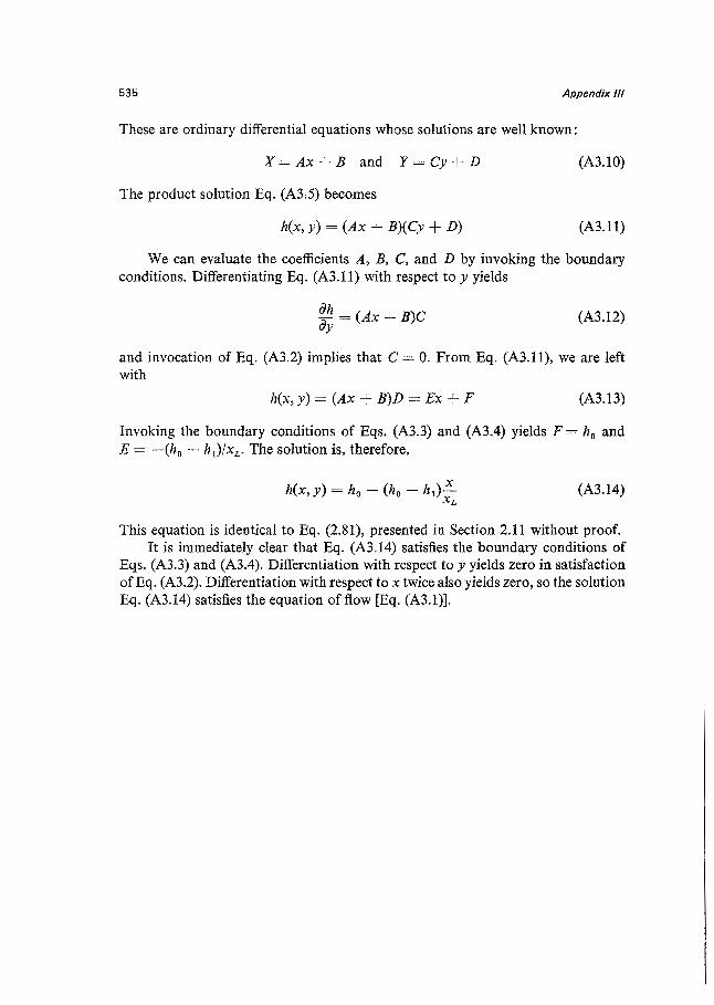
Invoking the boundary conditions of Eqs. (A3.3) and (A3.4) yields F = h0 and E = -(h0 - h1)/xL. The solution is, therefore,

(A3.14)

This equation is identical to Eq. (2.81), presented in Section 2.11 without proof. It is immediately clear that Eq. (A3.14) satisfies the boundary conditions of

Eqs. (A3.3) and (A3.4). Differentiation with respect toy yields zero in satisfaction of Eq. (A3.2). Differentiation with respect to x twice also yields zero, so the solution Eq. (A3.14) satisfies the equation of flow [Eq. (A3.l)].

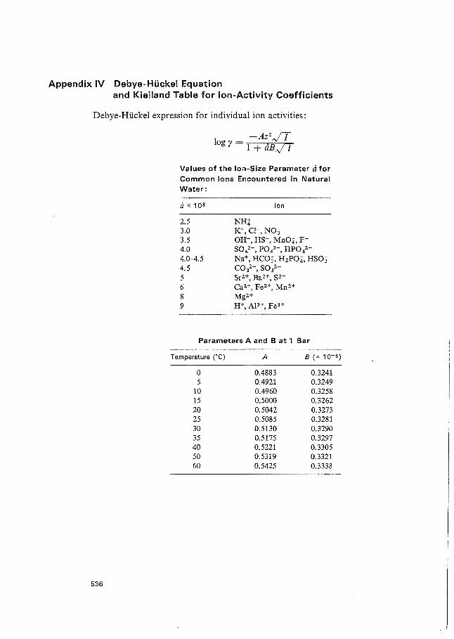
Appendix IV Debye-Hi.ickel Equation and Kielland Table for Ion-Activity Coefficients

Debye-Hlickel expression for individual ion activities:

536

_ -Az2,.JT log y - 1 + aB ,.j I

Values of the Ion-Size Parameter a for Common Ions Encountered in Natural Water:

a x 108

2.5 3.0 3.5 4.0 4.0-4.5 4.5 5 6 8 9

Ion

NHt K+, CI-, N03 OH-, HS-, Mn04, F­SOi-, P04

3-, HP042-

Na+, HC03, H2P04, HS03 co 3

2-, S032 -

sr2+, Ba2+, s2-ca2+, Fe2+, Mn2+ Mg2+ H+, Al3+, Fe3+

Parameters A and B at 1 Bar

Temperature (°C) A B ( x 10-8)

0 0.4883 0.3241 5 0.4921 0.3249

10 0.4960 0.3258 15 0.5000 0.3262 20 0.5042 0.3273 25 0.5085 0.3281 30 0.5130 0.3290 35 0.5175 0.3297 40 0.5221 0.3305 50 0.5319 0.3321 60 0.5425 0.3338

01 w -..J

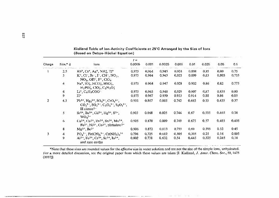
Kielland Table of Ion-Activity Coefficients at 25°C Arranged by the Size of Ions (Based on Debye-Huckel Equation)

/= Charge Size,* a Ions 0.0005 0.001 0.0025 0.005 0.01 0.025 0.05 0.1

2.5 Rb+, Cs+, Ag+, NH!, TI+ 0.975 0.964 0.945 0.924 0.898 0.85 0.80 0.75 3 K+, c1-, Be, 1-, cN-, N03, 0.975 0.964 0.945 0.925 0.899 0.85 0.805 0.755

NOz, OH-, F-, CI04 4 Na+, 103, HC03, HS03, 0.975 0.964 0.947 0.928 0.902 0.86 0.82 0.775

H2P04, CI02, C2H30z 6 Li+, C6HsCoo- 0.975 0.965 0.948 0.929 0.907 0.87 0.835 0.80 9 H+ 0.975 0.967 0.950 0.933 0.914 0.88 0.86 0.83

2 4.5 Pb2+, Hg22+, Soi-, Cr042-, 0.903 0.867 0.805 0.742 0.665 0.55 0.455 0.37 co3

2-, so32-, C2042-, S203

2-, H citrate2-

5 Sr2+, Ba2+, Cd2+, Hg2+, s2-, 0.903 0.868 0.805 0.744 0.67 0.555 0.465 0.38 W042-

6 Ca2+, Cu2+, zn2+, sn2+, Mn2+, 0.905 0.870 0.809 0.749 0.675 0.57 0.485 0.405 Fe2+, Ni2+, co2+, phthalate2-

8 Mg2+, Be2+ 0.906 0.872 0.813 0.755 0.69 0.595 0.52 0.45

3 4 pQ43-, Fe(CN)63-, Cr(NH3)6

3+ 0.796 0.725 0.612 0.505 0.395 0.25 0.16 0.095 9 AP+, Fe3+, Cr3+, Sc3 +, Jn3+, 0.802 0.738 0.632 0.54 0.445 0.325 0.245 0.18

and rare earths

*Note that these sizes are rounded values for the effective size in water solution and are not the size of the simple ions, unhydrated. For a more detailed discussion, see the original paper from which these values are taken [J. Kielland, J. Amer. Chem. Soc., 59, 1675 (1937)].

References

BERNER, R. A. 1971. Principles of Chemical Sedimentology. McGraw-Hill, New York, 240pp.

KLOTZ, I. M. 1950. Chemical Thermodynamics. Prentice-Hall, Englewood Cliffs, N. J., 369 pp.

MANOV, G. G., R. G. BATES, W. J. HAMER, and S. F. ACREE. 1943. Values of the con­stants in the Debye-Hilckel equation for activity coefficients. J. Amer. Chem. Soc., 65, pp. 1765-1767.

538

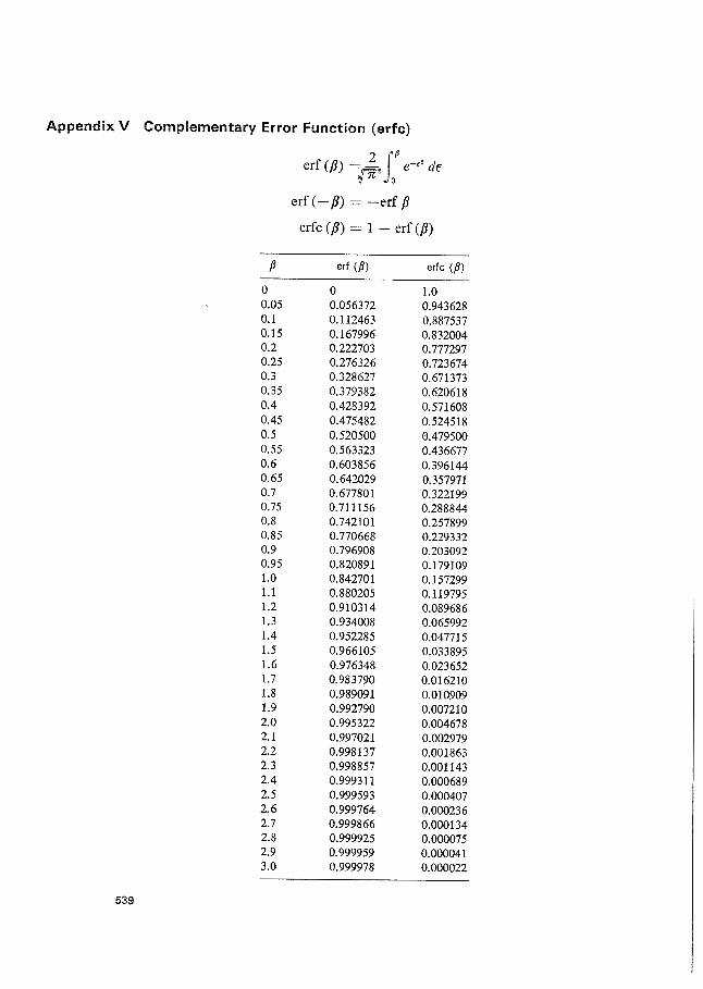
Appendix V Complementary Error Function (erfc)

2 lp erf (fi) = 0

e-E2 d€

erf (-p) = -erf p erfc (fi) = 1 - erf (p)

p erf <P) erfc (P)

0 0 1.0 0.05 0.056372 0.943628 0.1 0.112463 0.887537 0.15 0.167996 0.832004 0.2 0.222703 0.777297 0.25 0.276326 0.723674 0.3 0.328627 0.671373 0.35 0.379382 0.620618 0.4 0.428392 0.571608 0.45 0.475482 0.524518 0.5 0.520500 0.479500 0.55 0.563323 0.436677 0.6 0.603856 0.396144 0.65 0.642029 0.357971 0.7 0.677801 0.322199 0.75 0.711156 0.288844 0.8 0.742101 0.257899 0.85 0.770668 0.229332 0.9 0.796908 0.203092 0.95 0.820891 0.179109 1.0 0.842701 0.157299 1.1 0.880205 0.119795 1.2 0.910314 0.089686 1.3 0.934008 0.065992 1.4 0.952285 0.047715 1.5 0.966105 0.033895 1.6 0.976348 0.023652 1.7 0.983790 0.016210 1.8 0.989091 0.010909 1.9 0.992790 0.007210 2.0 0.995322 0.004678 2.1 0.997021 0.002979 2.2 0.998137 0.001863 2.3 0.998857 0.001143 2.4 0.999311 0.000689 2.5 0.999593 0.000407 2.6 0.999764 0.000236 2.7 0.999866 0.000134 2.8 0.999925 0.000075 2.9 0.999959 0.000041 3.0 0.999978 0.000022

539

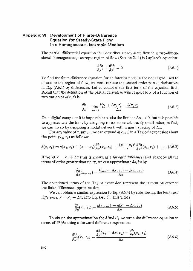
Appendix VI Development of finite-Difference Equation for Steady-State Flow in a Homogeneous, Isotropic Medium

The partial differential equation that describes steady-state flow in a two-dimen­sional, homogeneous, isotropic region of flow (Section 2.11) is Laplace's equation:

(A6.l)

To find the finite-difference equation for an interior node in the nodal grid used to discretize the region of flow, we must replace the second-order partial derivatives in Eq. (A6.1) by differences. Let us consider the first term of the equation first. Recall that the definition of the partial derivative with respect to x of a function of two variables h(x, z) is

ah = lim h(x + Ax, z) - h(x, z) ax Ax->O Ax

(A6.2)

On a digital computer it is impossible to take the limit as Ax ~ 0, but it is possible to approximate the limit by assigning to Ax some arbitrarily small value; in fact, we can do so by designing a nodal network with a mesh spacing of Ax.

For any value of z, say z0 , we can expand h(x, z0 ) in a Taylor's expansion about the point (x0 , z0 ) as follows:

_ ah (X - X0 ) 2 a2h h(x, Zo) - h(Xo, Zo) + (x - Xo) ax(Xo, Zo) + 2 ax2 (Xo, Zo) + ... (A6.3)

If we let x = x 0 +Ax (this is known as a forward difference) and abandon all the terms of order greater than unity, we can approximate ah/ax by

(A6.4)

The abandoned terms of the Taylor expansion represent the truncation error in the finite-difference approximation.

We can obtain a similar expression to Eq. (A6.4) by substituting the backward difference, x = x 0 - Lix, into Eq. (A6.3). This yields

ah ( ) h(Xo, Zo) - h(Xo - Lix, Zo) ax Xo, Zo = Ax (A6.5)

To obtain the approximation for a2h/ax2 , we write the difference equation in terms of ah/ ax using a forward-difference expression:

(A6.6)

540

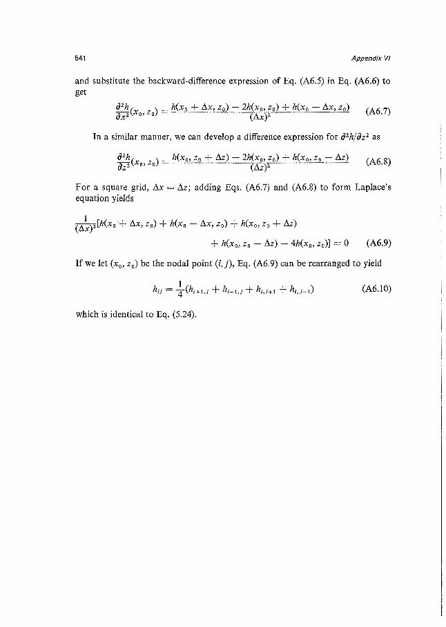
541 Appendix VI

and substitute the backward-difference expression of Eq. (A6.5) in Eq. (A6.6) to get

(A6.7)

In a similar manner, we can develop a difference expression for a2h/az2 as

(A6.8)

For a square grid, Ax = Az; adding Eqs. (A6. 7) and (A6.8) to form Laplace's equation yields

1 (Ax) 2 [h(xo +Ax, z0) + h(x 0 - Ax, z 0) + h(x 0 , z0 + Az)

+ h(x0 , Z 0 - Az) - 4h(x0 , z0 )] = 0 (A6.9)

If we let (x 0 , z0) be the nodal point (i,j), Eq. (A6.9) can be rearranged to yield

(A6.10)

which is identical to Eq. (5.24).

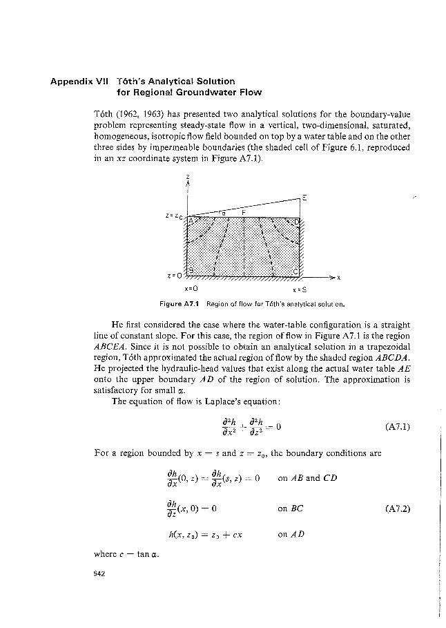
Appendix VII T6th's Analytical Solution for Regional Groundwater Flow

Toth (1962, 1963) has presented two analytical solutions for the boundary-value problem representing steady-state :flow in a vertical, two-dimensional, saturated, homogeneous, isotropic flow field bounded on top by a water table and on the other three sides by impermeable boundaries (the shaded cell of Figure 6.1, reproduced in an xz coordinate system in Figure A7.l).

x=O x =S

Figure A7.1 Region of flow for T6th's analytical solution.

He first considered the case where the water-table configuration is a straight line of constant slope. For this case, the region of :flow in Figure A 7. I is the region ABCEA. Since it is not possible to obtain an analytical solution in a trapezoidal region, Toth approximated the actual region of flow by the shaded region ABCDA. He projected the hydraulic-head values that exist along the actual water table AE onto the upper boundary AD of the region of solution. The approximation is satisfactory for small rx.

The equation of flow is Laplace's equation:

(A7.l)

For a region bounded by x = s and z = z0 , the boundary conditions are

ah ah ax(O, z} = ax(s, z) = 0 on AB and CD

ah az(x, 0) = 0 on BC (A7.2)

h(x, z0 ) = z 0 +ex on AD

where c = tan rx.

542

543 Appendix VII

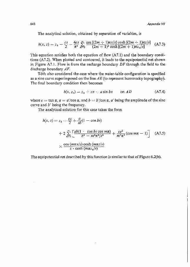
The analytical solution, obtained by separation of variables, is

h(x z) = z + cs _ 4cs i: cos [(2m + I)nx/s] cosh [(2m + I)nz/s] (A?.3) '

0 2 n 2 m=o (2m + 1)2 cosh [(2m + I)nz 0/s]

This equation satisfies both the equation of flow (A7.l) and the boundary condi­tions (A7.2). When plotted and contoured, it leads to the equipotential net shown in Figure A7.l. Flow is from the recharge boundary DF through the field to the discharge boundary AF.

Toth also considered the case where the water-table configuration is specified as a sine curve superimposed on the line AE (to represent hummocky topography). The final boundary condition then becomes

h(x, z 0 ) = z 0 + ex + a sin bx on AD (A7.4)

where c = tan et, a = a' /cos et, and b = b' /cos et, a' being the amplitude of the sine curve and b' being the frequency.

The analytical solution for this case takes the form

h(x, z) = z0 + c; + :b(l - cos bs)

+ 2 ~ [ab(I - cos bs cos mn) + cs2

(cos mn _ I)] (A7.5) m~l b2

- m2n 2/s2 m2n2

x cos (mnx/s) cosh (mnz/s) s • cosh (mnz 0 /s)

The equipotential net described by this function is similar to that of Figure 6.2(b ).

Appendix VIII Numerical Solution of the Boundary-Value Problem Representing One-Dimensional Infiltration Above a Recharging Groundwater Flow System

Consider a one-dimensional, vertical, homogeneous flow field with its upper boundary at the ground surface and its lower boundary below the water table. As outlined in Section 6.4, the equation of flow for such a system is

(A8.l)

and the boundary conditions are

(A8.2)

at the top, and

(A8.3)

at the base. The solution is in terms of the pressure head, 't.Jl(z, t). The position of the water table at any time is given by the value of z at which 't.fl = 0. The required input includes the initial conditions, 't.Jl(Z, 0), the rainfall rate R, the groundwater recharge rate Q, and the unsaturated characteristic curves K(rp) and C('t.f/). For 't.fl > 't.fl 0 , K = K 0 and C = 0, 't.fl 0 being the air entry pressure head.

The numerical finite-difference scheme used by Rubin and Steinhardt (1963), Liakopoulos (1965b), and Freeze (1969b) is the implicit scheme of Richtmyer (1957). With this method the (z, t) plane is represented by a rectangular grid of points j = 1, 2, ... , L along the z axis, and n = 1, 2, . . . along the t axis. The distance between the vertical nodes is Az, and between the time steps, At. The solu­tion at any given grid point (j, n) is 't.fli· Under this notation the finite-difference form for Eq. (AS.I) for an interior node (j = 2 to j = L - 1), after suitable rearrangement, is

CC't.f/m)('t.j/j ~ir1) = L {[ K('t.f/1)( 1 + 2lz['t.flj:~~ + 't.flj+1 - 't.jlj-1 - 't.fliJ) J - [ K('t.f/u)( I + 2l}'t.flj- 1 + 't.Jlj - 't.Jlj:~ - 't.f/j- 1]) ]} (A8.4)

where the values of 't.f/1' 't.f/m and 't.f/rm which determine the Kand C values to be applied for a particular node at a particular time step, are determined by extrapola­tion from previous time steps as described by Rubin and Steinhardt (1963).

Similar finite-difference equations, which incorporate the boundary conditions (A8.2) and (A8.3), can be written for the nodes at the upper and lower boundary (j= l,j=L).

544

545 Appendix VIII

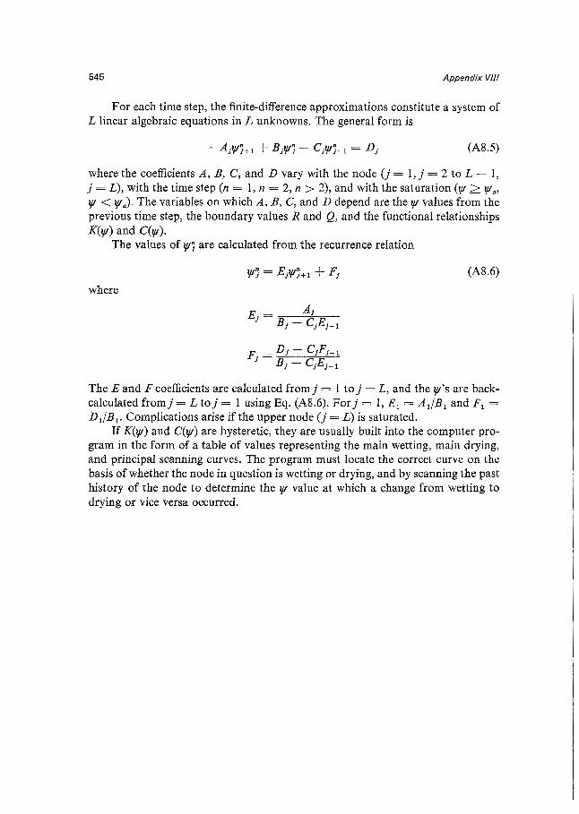
For each time step, the finite-difference approximations constitute a system of L linear algebraic equations in L unknowns. The general form is

(A8.5)

where the coefficients A, B, C, and D vary with the node(}= 1, j = 2 to L - 1, j = L), with the time step (n = 1, n = 2, n > 2), and with the saturation (lJI > lfla, lJI < lJI a). The variables on which A, B, C, and D depend are the lJI values from the previous time step, the boundary values Rand Q, and the functional relationships K(lJI) and C(lJI).

The values of lfli are calculated from the recurrence relation

(A8.6)

where

The E and F coefficients are calculated from}= 1 to j = L, and the lJl'S are back­calculated from}= L to}= 1 using Eq. (A8.6). For}= 1, £ 1 = A1/B 1 and F 1 = D 1/B 1• Complications arise if the upper node (j = L) is saturated.

If K(lJI) and C{lJI) are hysteretic, they are usually built into the computer pro­gram in the form of a table of values representing the main wetting, main drying, and principal scanning curves. The program must locate the correct curve on the basis of whether the node in question is wetting or drying, and by scanning the past history of the node to determine the lJI value at which a change from wetting to drying or vice versa occurred.

Appendix IX Development of Finite-Difference Equation for Transient Flow in a Heterogeneous, Anisotropic, Horizontal, Confined Aquifer

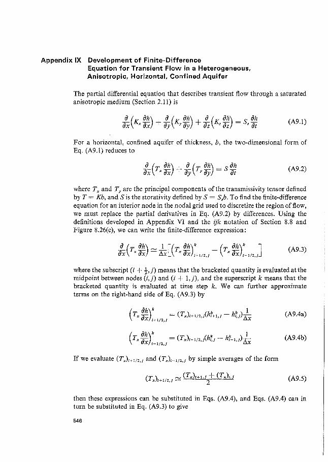
The partial differential equation that describes transient flow through a saturated anisotropic medium (Section 2.11) is

j_(K ah)+ j_(K ah)+ j_(K ah)_ s ah ax x ax ay y ay az z az - s at (A9.l)

For a horizontal, confined aquifer of thickness, b, the two-dimensional form of Eq. (A9.l) reduces to

(A9.2)

where Tx and Ty are the principal components of the transmissivity tensor defined by T = Kb, and Sis the storativity defined by S = Ssh. To find the finite-difference equation for an interior node in the nodal grid used to discretize the region of flow, we must replace the partial derivatives in Eq. (A9.2) by differences. Using the definitions developed in Appendix VI and the ijk notation of Section 8.8 and Figure 8.26(c), we can write the finite-difference expression:

j_ (T ah) ,.....,,, _1 [(T ah)k _ (T ah)k J ax x ax - 8x x ax i+l/2,J x ax i-1/2,J

(A9.3)

where the subscript (i + f,j) means that the bracketed quantity is evaluated at the midpoint between nodes (i,j) and (i + l,j), and the superscript k means that the bracketed quantity is evaluated at time step k. We can further approximate terms on the right-hand side of Eq. (A9.3) by

( TX aaxh)k = (Tx)t+112,iM+1,1 - ht1) }x i+l/2,J il

(A9.4a)

( TX aah)k = (TJt-112.iht1 - M-1,1)} X i-1/2,J ilX

(A9.4b)

If we evaluate (Tx)i+ 1; 2,1 and (Tx)t_ 112,1 by simple averages of the form

(T) ,....., (Tx)t+1.1 + (TJt,J x i+1/2,j - 2 (A9.5)

then these expressions can be substituted in Eqs. (A9.4), and Eqs. (A9.4) can in turn be substituted in Eq. (A9.3) to give

546

547

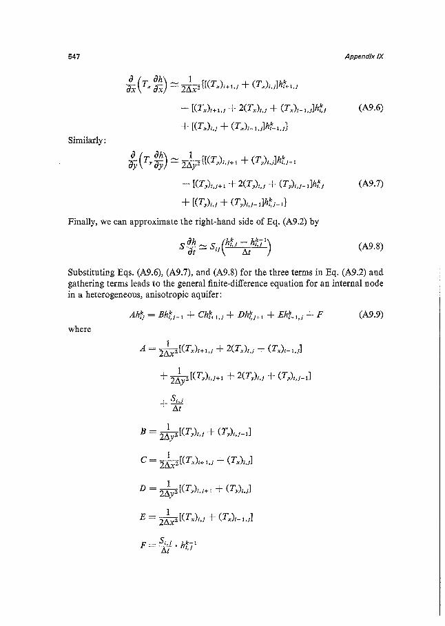
Similarly:

:X ( Tx ~~)::::::: 2lx2 {[(Tx)i+1,l + (Tx)i,1]hf+1,J

- [(Tx)i+1,l + 2(Tx)i,J + (Tx)i-1,l]hf.1

+ [(Tx)i,l + (Tx)1-1.1lM-1,1}

~ (Ty~~) ::::::: 2ly2 {[(Ty)t,1+1 + (Ty)t,1]hf.1+1

- [(Ty)t,J+1 + 2(Ty)t,1 + (Ty)t,1-1]hf1

+ [(Ty)t,1 + (Ty)t,1-1]ht1-d

Finally, we can approximate the right-hand side of Eq. (A9.2) by

Appendix IX

(A9.6)

(A9.7)

(A9.8)

Substituting Eqs. (A9.6), (A9.7), and (A9.8) for the three terms in Eq. (A9.2) and gathering terms leads to the general finite-difference equation for an internal node in a heterogeneous, anisotropic aquifer:

where

Ahi = Bht1- 1 + Chf+ 1,1 + Dhf.1+1 + Ehf- 1,1 + F

1 A= 2L\x2[(Tx)i+l,l + 2(Tx)l,l + (Tx)t-1,1]

1 + 2L\y2[(Ty)t,1+1 + 2(Ty)t,1 + (Ty)t,1-1]

+ S1.1 L\t

1 B =

2L\y2 [(Ty),,1 + (Ty)1,1_ i]

1 C = 2L\xz[(TJ1+1,1 + (Tx)1,1]

1 D = 2L\y2[(Ty)1,J+1 + (Ty),,1]

1 E = 2L\x2[(Tx)i,l + (Tx)i-1,1]

F _Su hk-1 -Yt. i,l

(A9.9)

548 Appendix IX

If the aquifer is homogeneous and isotropic, then Tx = Ty= T for all (i,j) and Si,J = S for all (i,j). Under these conditions, and for a square nodal grid with Lix = Liy, the coefficients of Eq. (A9.9) become

A= 4T + Si, 1

Ax2 Lit

T B=C=D=E=­Lix2

If we divide through by T/ Lix2, these coefficients are seen to be the same as those developed in a less rigorous way in Section 8.8 and presented in connection with Eq. (8.57).

Trescott et al. (1976) have suggested that there is some advantage to utilizing the harmonic mean rather than the arithmetic mean in Eq. (A9.5). This approach changes the coefficients in the finite-difference equation but does not alter the con­cepts underlying the development.

Equation (A9.9) is written in terms of the hydraulic head values at five nodes at time step k and one node at time step k - 1. It is known as a backward-difference approximation. Remson et al. (1971) note that there are some computational advantages to using a central-difference approximation, known as the Crank­Nicholson scheme, that utilizes head values at five nodes at time step k and five nodes at time step k - 1. The alternating-direction implicit procedure (ADIP) utilized by Pinder and Bredehoeft (1968) involves two finite-difference equations, one in the xt plane and one in the yt plane. Each uses head values at three nodes at time step k and three nodes at time step k - 1.

Appendix X Derivation of the Advection-Dispersion Equation for Solute Transport in Saturated Porous Media

The equation derived here is a statement of the law of conservation of mass. The derivation is based on those of Ogata (1970) and Bear (1972). It will be assumed that the porous medium is homogeneous and isotropic, that the medium is satu­rated, that the flow is steady-state, and that Darcy's law applies. Under the Darcy assumption, the flow is described by the average linear velocity, which carries the dissolved substance by advection. If this were the only transport mechanism opera­tive, nonreactive solutes being transported by the fluid would move as a plug. In reality, there is an additional mixing process, hydrodynamic dispersion (Section 2.13), which is caused by variations in the microscopic velocity within each pore channel and from one channel to another. If we wish to describe the transport process on a macroscopic scale using macroscopic parameters, yet take into account the effect of microscopic mixing, it is necessary to introduce a second mechanism of transport, in addition to advection, to account for hydrodynamic dispersion.

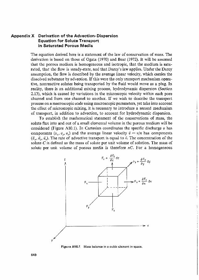
To establish the mathematical statement of the conservations of mass, the solute flux into and out of a small elemental volume in the porous medium will be considered (Figure AIO. l). In Cartesian coordinates the specific discharge v has components (vx, Vy, vz) and the average linear velocity v = v/n has components (vx, Vy, vz). The rate of advective transport is equal to v. The concentration of the solute C is defined as the mass of solute per unit volume of solution. The mass of solute per unit volume of porous media is therefore nC. For a homogeneous

y

549

z

//

/

/

I I I .J.-.--- ---

Figure A10.1 Mass balance in a cubic element in space.

550 Appendix X

medium, the porosity n is a constant, and a(nC)/ax = n ac;ax. The mass of solute transported in the x direction by the two mechanisms of solute transport can be represented as

transport by advection = vxnC dA (AlO.l)

transport by dispersion= nDx ~; dA (Al0.2)

where Dx is the dispersion coefficient in the x direction and dA is the elemental cross-sectional area of the cubic element. The dispersion coefficient Dx is related to the dispersivity rxx and the diffusion coefficient D* by Eq. (9.4):

(Al0.3)

The form of the dispersive component embodied in Eq. (AI0.2) is analogous to Fick's first law.

If Fx represents the total mass of solute per unit cross-sectional area transported in the x direction per unit time, then

Fx = VxnC - nDx ~; (Al0.4)

The negatiye sign before the dispersive term indicates that the contaminant moves toward the zone of lower concentration. Similarly, expressions in the other two directions are written

(Al0.5)

(AI0.6)

The total amount of solute entering the cubic element (Figure AlO.l) is

Fx dz dy + F,, dz dx + Fz dx dy

The total amount leaving the cubic element is

where the partial terms indicate the spatial change of the solute mass in the specified direction. The difference in the amount entering and leaving the element is, there­fore,

551 AppendixX

Because the dissolved substance is assumed to be nonreactive, the difference between the flux into the element and the flux out of the element equals the amount of dissolved substance accumulated in the element. The rate of mass change in the element is

ac -n-dxdydz at

The complete conservation of mass expression, therefore, becomes

(Al0.7)

Substitution of expressions (Al0.4), (Al0.5), and (Al0.6) in (Al0.7) and cancella­tion of n from both sides yields:

[ a (D ac) + a (D ac) + a (D ac)J ax x ax ay y ay az z az

(AI0.8)

In a homogeneous medium in which the velocity iJ is steady and uniform (i.e., if it does not vary through time or space), dispersion coefficients D.r, Dy, and D, do not vary through space, and Eq. (Al0.8) becomes

(AI0.9)

In one dimension,

D a2c _ v ac = ac x ax2 x ax at (AI0.10)

In some applications, the one-dimensional direction is taken as a curvilinear coordinate in the direction of flow along a flowline. The transport equation then becomes

(AI0.11)

where I is the coordinate direction along the flow line, D1 the longitudinal coefficient of dispersion, and v1 the average linear velocity along the flowline.

552 Appendix X

For a two-dimensional problem, it is possible to define two curvilinear coordi­nate directions, Si and Sn where Sz is directed along the flowline and Sc is orthogo­nal to it. The transport equation then becomes

(AI0.12)

where Dz and De are the coefficients of dispersion in the longitudinal and transverse directions, respectively.

If Vz varies along the flow line and Dz and Dr vary through space, Eq. (Al 0.13) becomes

(AI0.13)

Equations (AI0.8) through (Al0.13) represent six forms of the advection­dispersion equation for solute transport in saturated porous media. Equation (Al 0.11) is identical to Eq. ( 9 .3) in Section 9 .2. The solution to any one of these equations will provide the solute concentration C as a function of space and time. It will take the form C(x, y, z, t) for Eqs. (Al0.8) and (Al0.9); C(l, t) for Eq. (A10.ll);andC(S1,S1,t) forEqs. (Al0.12) and (Al0.13). There are many well known analytical solutions to the simpler forms of the transport equation. Equation (9.5) in Section 9.2 is an analytical solution to Eq. (Al0.11 ), and Eq. (9.6) is an analytical solution to Eq. (Al0.9). In most field situations, two- or three-dimen­sional analyses are required. In addition, the velocities are seldom uniform and the dispersivities are usually variable in space. For these conditions, numerical methods adapted for digital computers must be used to obtain solutions.

The coefficient of dispersion in a three-dimensional, homogeneous, isotropic porous medium as expressed in Eq. (AI0.12) is a second-order symmetrical tensor with nine components. Di and Dt are the diagonal terms of the two-dimensional form. The directional properties of the dispersion coefficient are caused by the nature of the dispersive process in the longitudinal and transverse directions. If the medium is itself anisotropic, mathematical description of the dispersive process takes on much greater complexity. No analytical or numerical solutions are avail­able for anisotropic systems. Only for isotropic media has the coefficient of disper­sion been represented successfully by experimental methods.

It is possible to extend the transport equation to include the effects of retarda­tion of solute transport through adsorption, chemical reaction, biological transfor­mations, or radioactive decay. In this case the mass balance carried out on the elemental volume must include a source-sink term. For retardation due to adsorp­tion, the transport equation in a homogeneous medium in a one-dimensional system along the direction of flow ta~es the form

D azc - ac + Pb as _ ac i a/2 - Vz at n at - at (Al0.14)

553 Appendix X

where Pb is the bulk mass density of the porous medium, n the porosity, and S the mass of chemical constituent adsorbed on a unit mass of the solid part of the porous medium. The first term of Eq. (Al0.14) is the dispersion term, the second is the advection term, and the third is the reaction term. This form of the reaction term is considered in Section 9.2 in connection with Eqs. (9.9) through (9.13). Analytical solutions to Eq. (Al0.14) are presented by Codell and Schreiber (in press). Figure 9.12 presents some sample solutions carried out by Pickens and Lennox (1976) using numerical methods.