Embed Size (px)
Citation preview

Appendix I Molecular biological methods ............................................................... I
I.1 An optimised protocol for rapid DNA extraction from European
flounder tissues. ......................................................................................................... I
I.1.1 DNA Extraction protocol – European flounder ...................................... I
I.2 Spectrophotometric quantification of nucleic acids................................ III
I.3 First strand cDNA synthesis (reverse transcription) .............................. IV
I.4 1st strand cDNA Purification using QIAquick spin columns (Qiagen) ...V
I.5 Agarose gel electrophoresis of RNA prior to Northern Blotting ........... VI
I.6 Northern (& Southern) blotting .................................................................VII
I.7 Probing / hybridisation of filters - Northern or Southern blot ............. VIII
I.7.1 Probe preparation and labelling ......................................................... VIII
I.7.2 Filter preparation ..................................................................................... IX
I.8 Transformation protocol using ‘Top 10’ competent cells .....................XII
I.9 Plating out of colonies – from (Sambrook et al., 1999) ...................... XIII
I.9.1 Day one.................................................................................................. XIII
I.9.2 Day two .................................................................................................. XIII
I.9.3 Day three ............................................................................................... XIV
I.10 Probing / hybridisation of filters – bacterial colony screening .............XV
I.11 Pouring and running a Polyacrylamide gel, and gel electrophoresis.
XVII
I.12 Sequencing of plasmid construct........................................................... XIX
I.13 Direct sequencing of PCR product ..........................................................XX
I.14 Big Dye sequencing clean up method – Sanger Centre.................... XXI
I.15 Protocol for colony PCR.........................................................................XXII
Appendix II Microsatellite data: Chapter 3 ......................................................XXIII
II.1 Microsatellite sequences.......................................................................XXIII
II.2 Inheritance of microsatellites – Allele data........................................ XXIX
Appendix III The European flounder CYP1A gene ................................... XXXII
III.1 Platichthys flesus cDNA for Cytochrome P4501A (annotated)..... XXXII
APPENDICES
III.2 Statistical results for chapter 5 ..........................................................XXXIII
III.2.1 Regression analysis of physical characteristics and Ah battery
gene expression ..........................................................................................XXXIII
III.3 Raw data for Aroclor 1254 trial .........................................................XXXIV
III.3.1 Aroclor exposed flounder ...........................................................XXXIV
III.3.2 Control flounder ...........................................................................XXXVI
Appendix IV Recipes ..................................................................................XXXVIII
IV.1 Buffers................................................................................................XXXVIII
IV.2 Bacterial Media ........................................................................................ XLII
IV.3 Formulae: ................................................................................................XLIV
Appendix V Real-time PCR................................................................................. XLV
V.1 AhR2 standard curve .............................................................................. XLV
V.2 ARNT2 standard curve..........................................................................XLVI
This document is © Tom Dixon, 2003 http://www.tomdixon.org
2
APPENDIX I – MOLECULAR BIOLOGY METHODS
Appendix I Molecular biological methods
I.1 An optimised protocol for rapid DNA extraction from European flounder tissues.
Extensive optimisations were carried out to find a DNA extraction method which
would produce good quality (high molecular weight) DNA from a variety of European
flounder (Platichthys flesus) tissues including liver and fin clips. Investigations were
carried out based on two protocols for DNA extraction, one from Atlantic salmon
(Taggart et al., 1992), and another from mouse tail (Mullins traditional DNA
extraction). The following protocol was therefore optimised, and all DNA extractions
used throughout this study used this method of extraction (with the exception of larval
DNA extraction – details provided in Chapter 3). Provided all materials and solutions
are sterile and autoclaved where appropriate, high molecular weight DNA was
regularly extracted and was suitable for PCR and RE digest etc.
I.1.1 DNA Extraction protocol – European flounder
Materials required:
Solution: 1. 50mM Tris HCl; pH8.0, 10mmM EDTA, 100mM NaCl, 1% v/v SDS 2. Proteinase K, 20mg/ml 3. RNase (Dnase free), 20mg/ml 4. Phenol, pH 8.0 equilibrated 5. Chloroform:isoamyl alcohol 24:1 6. 70% Ethanol 7. TE pH 8.0 (100mM Tris, 1mM EDTA) - Sterile 8. Isopropanol Method
Day 1:
1. Add 375µL solution 1 + 12µL proteinase K to a clean eppendorf
2. Add fin clip / tissue (ca. 5-10mm) to each tube
3. Incubate overnight at 55°C in a shaking incubator or rottiserie oven with
constant agitation.
I

APPENDIX I – MOLECULAR BIOLOGY METHODS
Day 2:
1. Add 10µl RNase to each tube and invert gently to mix. Incubate for one hour at
37°C (waterbath or oven).
2. Add 400µL phenol to each tube. Mix by over-end turning for 15-20 mins.
3. Add 400µL chloroform:isoamyl alcohol to each tube. Mix by over-end turning
for 15-20 mins.
4. Centrifuge the tubes at 10,000 x g for 5 mins.
5. Remove 300µLs of the top aqueous layer to a clean microfuge tube using pre-
cut wide bore Gilson tips.
6. Add 400µLs cold isopropanol (or 600µLs absolute ethanol) to precipitate the
DNA. Invert several times, and incubate at –20°C for 30 mins (if using ethanol
to precipitate DNA, leave at room temperature for 30mins).
7. Centrifuge microfuge tube at 12,000g for 10mins to pellet the DNA.
8. Decant off most ethanol.
9. Add 1ml 70% ethanol to wash the DNA. Mix by gentle over-end turning for
30mins. Centrifuge at 12,000g for 10mins, and remove ethanol.
10. Allow DNA to air dry at room temperature for 5-10mins until all remaining
ethanol has evaporated.
11. Resuspend pellet in 100µL molecular biology grade water. Total dissolution
often takes several days at 4°C. Store at 4°C, or –20°C for long term storage.
II

APPENDIX I – MOLECULAR BIOLOGY METHODS
I.2 Spectrophotometric quantification of nucleic acids
Nucleic acids were quantified using a DNAamp spectrophotometer (Pharmacia). An
aliquot of the nucleic acid (RNA or DNA) was removed from the extracted sample, and
diluted to the appropriate factor in molecular biology grade water (BDH). The same
water was used as a blank to calibrate the spectrophotometer prior to first use. After
every 10th sample quantified, a reading was taken from the molecular grade water.
Assuming a value of zero was returned, the machine was accurate, and the results were
accepted. Quantity of dsDNA or RNA was calculated using the following calculation:
Abs260 x nucleic acid quantification coefficient* x dilution factor = Concentration of
DNA RNA in original sample
*(DNA = 50, RNA = 40)
Quality of the DNA and RNA was checked using the Abs260 / Abs280 ratio.
III

APPENDIX I – MOLECULAR BIOLOGY METHODS
I.3 First strand cDNA synthesis (reverse transcription)
Reverse transcription was carried out to synthesise first strand cDNA from an RNA
template. The method presented below using Moloney Murine Leukaemia Virus
(MMLV) Reverse Transcriptase (Promega Inc.), and poly T primers (to select all
mRNA) is based on standard protocols (Promega technical data as supplied; &
(Sambrook et al 1996)). Poly T primer was synthesised by MWG Biotech, sequence
T(16)V.
• To a 200µl PCR tube, add:
Stock Volume
1µg total RNA 1µg.µl stock 1µl
500ng (76pmols) poly T primer 7pmol.µl stock 11µls
Total 12µls
• Incubate at 70oC for 5 mins, then place on ice. Add the following reagents:
Stock Volume
5x RT buffer 5x 4µls
dNTP 10mM 1µl
dH20 2µls
Total 19µls
• Incubate at 42 deg for 5 min
• Add 1µl (200 U) MMLV H- Reverse Transcriptase (200 U.µl)
• Incubate for a further 50 mins at 42°C.
Place on ice if using immediately, otherwise store at –40°C.
IV

APPENDIX I – MOLECULAR BIOLOGY METHODS
I.4 1st strand cDNA Purification using QIAquick spin columns (Qiagen)
The protocol follows manufacturers instructions as detailed below. All samples for
comparison were prepared using the same batch of kit & reagents to ensure consistency
of reaction.
1. Five volumes (50µL) of binding buffer were added to 10µl of RT reaction, and
the whole mix transferred to a purification column.
2. Columns were spun at 12,000 RPM for one minute to allow binding of the
solutions to the column matrix.
3. 0.75ml of Wash buffer were added to remove impurities from the sample, and
re-spun at 12,000 RPM for two minutes.
4. Columns were transferred to clean Eppendorfs, and an appropriate volume
(100µL) of TE (pH8.0 1/10th EDTA) was added to the centre of the column.
Samples were eluted in the maximum possible volume to increase yield
efficiencies (see Qiagen data). At 100µL elution volume, efficiency is
consistently 90% (QIAgen).
5. Columns were re-spun at 12,000 RPM for 2 mins to recover the sample.
6. Samples were then stored at –20oC until required.
V
APPENDIX I – MOLECULAR BIOLOGY METHODS
I.5 Agarose gel electrophoresis of RNA prior to Northern Blotting
A midi-gel (13×15×1cm, Amersham Pharmacia, UK) casting tray was prepared, and
the desired number of 16-well combs inserted. To a conical flask was added:
1.3g Agarose
4.8 ml 25x MOPS buffer
126 ml dH2O
The above was then heated in a microwave at full power for two minutes, and allowed
to boil to dissolve the agarose. The gel was then allowed to cool to 50°C, before
addition of 40µl 10mg/ml ethidium bromide. The gel was immediately cast into the
prepared tray, and allowed to set for approximately 20 minutes. Once the gel was fully
set, combs were removed. The gel was then immersed in 700mls of 1× MOPS running
buffer, samples were loaded, and electrophoresed for the appropriate time (between
30mins – 1hour) at 4V/cm.
VI
APPENDIX I – MOLECULAR BIOLOGY METHODS
I.6 Northern (& Southern) blotting
A plastic tray was half filled with 20xSSC. Onto the plastic tray was placed a glass
sheet, with Whatman 3mm blotting paper soaked in 20xSSC wrapped around to act as a
wick. Either end of the blotting paper was placed into the tray containing 20xSSC to
allow the buffer to soak up by capillary action. The agarose gel (RNA or cDNA PCR)
was laid onto the blotting paper face down, and a plastic mask (Saran wrap) was then
placed around the gel to prevent any short-circuiting between the wick and the
absorbent material above. Hybond ‘N’ membrane was used as the filter. The filter was
marked on the top side with pencil, and the top right hand corner cut off to verify
orientation. This was cut to size, then laid over the gel, being careful to avoid getting
any air bubbles trapped between the filter and gel which would cause inefficient, and
possibly uneven, transfer of RNA. Once the filter was in place, eight sheets of
Whatman 3mm paper, equal in size to the gel, were placed on top, and a stack of paper
tissues added above that. The absorbent stack was to allow capillary diffusion of the
RNA from the gel onto the Nylon filter. Finally, a second glass plate, and a 500gm
weight were placed onto the top of the stack to compress the layers sufficiently to allow
soaking up of the SSC.
Once assembled, the blot was left overnight (ca 20hrs) to allow complete transfer of the
RNA / DNA. After blotting was complete, the assembly was dismantled, and the gel
visualised under UV light to ensure total transfer had occurred.
Filter preparation
Filters were removed and washed in 2x SSC to remove any agarose debris and
excessive salts. Filters were then placed between fresh Whatman 3MM paper and air
dried. Once dry, filters were baked for 60mins at 80oC to fix the RNA. Once fixed,
filters remain stable for several months if stored in dry, dark conditions (Dyson, 1991).
VII

APPENDIX I – MOLECULAR BIOLOGY METHODS
I.7 Probing / hybridisation of filters - Northern or Southern blot
I.7.1 Probe preparation and labelling
Generation of probe fragment
Plasmid containing the required probe was transformed into Top 10 competent cells
according to standard protocols (see I.8). Colonies were grown up over night on LB
(100µg/ml ampicillin) plates at 37oC. Single colonies were then picked, and cultures
grown up over night in 3ml of LB Amp broth at 37oC. Plasmids were then purified out
of the cultures using GFX plasmid preparation kits (Amersham Pharmacia) according
to the manufacturer’s protocol. Plasmids were checked by restriction digest, and sizing
of fragments on 1.2% agarose (1xTAE gels). Once sizing was confirmed as correct,
probe fragments were generated by cutting the required DNA out of the appropriate
plasmid using the relevant restriction enzymes (see individual probe descriptions for
details). Restriction digests were stopped with heat denaturation of the enzyme at the
relevant temperature, and aliquots of the reaction were run on low melting point
agarose gels. Bands were excised from gels using a scalpel, and purified using GFX gel
band purification kits (Amersham Pharmacia) according to manufacturers protocol. The
purified products were then eluted in dH2O, and quantified spectrophotometrically, and
on agarose. Twenty five nanograms of probe fragment was then used in the labelling
reaction.
Probe labelling reaction
All probes were labelled with α32P dCTP (4000 Ci / mmol; 10µCi/µl) using a ‘random
primers DNA labelling kit’ (Gibco BRL) according to manufacturers protocol. Briefly:
• Twenty five nanograms of probe DNA was diluted in 5-25µl BDH dH2O in a
screw-cap 1.5ml microcentrifuge tube. DNA was denatured for 5 min in a
boiling water bath, then immediately transferred to ice.
VIII
APPENDIX I – MOLECULAR BIOLOGY METHODS
• While on ice, the following components were added to the microcentrifuge tube
from the ‘Random primers DNA labelling kit’:
2µl dATP soln.
2µl dGTP soln
2µl dTTP soln
15µl random primers buffer mix
5µl (50µCi) α32P dCTP (4000 Ci / mmol; 10µCi/µl)
dH2O to a total vol. Of 49µl
• The solution was mixed briefly, and 1µl Klenow fragment (as supplied) added.
Solution was then mixed again, and spun down in centrifuge to collect it at the
base of the tube. The reaction mix was then incubated for 1 hr at 25oC.
• After one hour incubation, 5 µl stop buffer was added, then the probe purified
using ProbeQuantTM G-50 Micro Columns (Amersham Pharmacia) according to
manufacturers protocol to remove any unincorporated isotope.
Prior to hybridisation, the probe was denatured for 5 mins in a boiling water bath.
I.7.2 Filter preparation
Pre-hybridisation of filters
Filters were soaked in 2x SSC, then rolled out into a Techne hybridisation tube. Where
necessary, two to three filters were probed per tube. In this case, a nylon mesh was
placed between the filters, and between the outer filter and the tube to prevent air
bubbles from becoming trapped, and the filters from sticking together and cause non-
uniform probe binding. Twenty-five ml of modified Church buffer (hybridisation
solution) (3.5g SDS; 49mls 0.5M Na phosphate buffer, pH 7.2; 1ml 0.5M EDTA) was
added to each tube, and hybridisation tubes were transferred to a rotisserie style oven
(Techne). Filters were pre-hybridised at appropriate temperature (see individual probe
details) in the hybridisation tubes for a minimum of three hours in order to reduce
background noise during probe hybridisation.
IX
APPENDIX I – MOLECULAR BIOLOGY METHODS
Hybridisation protocol
Once the filters were suitably pre-hybridised, the pre-hybridisation wash fluid was
discarded. The purified and denatured labelled probe was added to 25ml Church buffer,
and the solution added to the hybridisation tube containing the membranes. The probe
was then hybridised to the filter by overnight incubation at appropriate temperature in a
Techne rotisserie oven.
Post hybridisation washes of filters
Each of the following solutions was made up prior to washing of filters. As the
stringency of washes varied between probes, counts per second (cps) readings were
taken after each wash using a hand-held mini-monitor.
200 mls 2X SSC; 0.1% SDS
200 mls 1X SSC; 0.1% SDS
100 mls 0.5X SSC; 0.1%SDS
Washes were carried out specific to each probe (see chapters for details).
Autoradiographic exposure
After washes were completed, transfer membranes were blotted dry on Whatman 3MM
paper and wrapped in Saran wrap™. The wrapped transfer membranes were placed in a
film cassette with an intensifying screen and autoradiography film (Kodak) (orientation
marked by cutting the top right hand corner). The cassette was then placed at -70°C for
overnight exposure, and was removed thirty minutes prior to developing film.
Autoradiograms were developed, and dried for thirty minutes in a drying cabinet. After
developing autoradiograms, images were scanned using an Epson GT2000 flatbed
scanner. Images were analysed via densitometry as e.g. (Kaplan, et al.,(1995));
(Courtenay et al., (1999)) using ‘gel capture’ macros in Scion Image analysis (based on
NIH Image analysis software (Bethesda, MD, USA)) and the intensities recorded as
relative mean expression, as described by (Courtenay et al., (1999)).
X

APPENDIX I – MOLECULAR BIOLOGY METHODS
Strip filters:
Filters were then stripped by removing from SARAN wrap, and placing in a 0.1% SDS
solution at95°C. The solution containing filter was then allowed to cool to room
temperature.
XI
APPENDIX I – MOLECULAR BIOLOGY METHODS
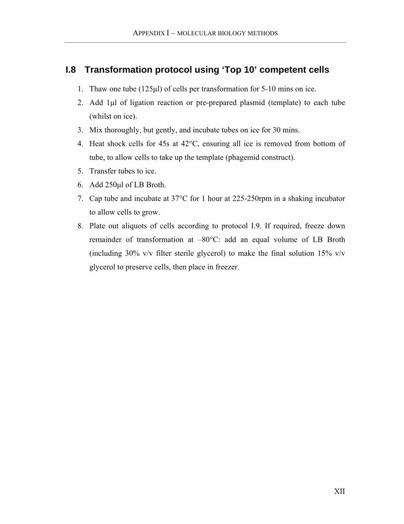
I.8 Transformation protocol using ‘Top 10’ competent cells
1. Thaw one tube (125µl) of cells per transformation for 5-10 mins on ice.
2. Add 1µl of ligation reaction or pre-prepared plasmid (template) to each tube
(whilst on ice).
3. Mix thoroughly, but gently, and incubate tubes on ice for 30 mins.
4. Heat shock cells for 45s at 42°C, ensuring all ice is removed from bottom of
tube, to allow cells to take up the template (phagemid construct).
5. Transfer tubes to ice.
6. Add 250µl of LB Broth.
7. Cap tube and incubate at 37°C for 1 hour at 225-250rpm in a shaking incubator
to allow cells to grow.
8. Plate out aliquots of cells according to protocol I.9. If required, freeze down
remainder of transformation at –80°C: add an equal volume of LB Broth
(including 30% v/v filter sterile glycerol) to make the final solution 15% v/v
glycerol to preserve cells, then place in freezer.
XII

APPENDIX I – MOLECULAR BIOLOGY METHODS
I.9 Plating out of colonies – from (Sambrook et al., 1999)
I.9.1 Day one
• Pour 30ml of prepared agar (100µg/ml ampicillin), per 90mm plate.
• Dry for 5mins upright with lid removed. Invert and dry for 40mins with lid
removed (at 37°C).
• 100µl of 100mM IPTG and 1.2µl 40mg/ml X-Gal were spread onto the top surface
of the plates to allow colour selection.
• Plates were dried for 5mins upright, and 40mins inverted in a 37°C oven.
• Transformation were then plated out by pipetting the required amount onto the
centre of the prepared agar plate, and spread uniformly across the plate using a
sterile plate spreader: Initially using dilutions;
1µl transformation in 99µl NZY+ broth
10µl transformation in 90µl NZY+ broth.
• Plates were dried upright for 5 mins at 37°C, and wrapped in ParafilmTM. Plates
were inverted, and incubated at 37°C for c.17hrs.
I.9.2 Day two
• Incubate plates at 4°C for 2 hrs to enhance blue colour (if using blue / white
selection).
• Colonies without inserts will appear blue, colonies with inserts will remain white.
• Once required colonies have been identified, single examples can be picked and
transferred to 3ml of LB Broth (100µg/ml ampicillin) in sterile universals. These
colonies are then grown up overnight (approx 16hrs) in a shaking incubator at 37°C
with constant rotation.
XIII

APPENDIX I – MOLECULAR BIOLOGY METHODS
I.9.3 Day three
• Once adequate growth was observed, universals were removed from the incubator,
and cells pelleted. The aqueous LB Broth was then removed, and plasmid
preparations carried out as required.
XIV

APPENDIX I – MOLECULAR BIOLOGY METHODS
I.10 Probing / hybridisation of filters – bacterial colony screening
Colony screenings were performed in order to detect positive colonies during
microsatellite enrichment (i.e. those colonies containing a microsatellite insert)(see
Chapter Three). The method presented below was used for both colony lifts, and colony
screenings from 96 well plates, and involve fixing the bacterial (plasmid) DNA onto
Hybond N (Amersham, UK) membrane.
Lysing of bacterial colonies and fixing of DNA to membrane
Filters were removed from agar plates, and denatured by placing them on Whatman
3MM paper (soaked in denaturing solution) for 8mins. The filters were then transferred
to clean Whatman 3mm paper (soaked in neutralising solution) for 2 x 4 minute washes
to neutralise them. The filters were then baked at 80oC for 2 hours to fix the DNA to the
membrane. (For full details of denaturing and neutralising solution, please see
‘Recipes’ section).
Filter preparation
Prior to hybridisation, filters were soaked overnight in 6X SSC (0.1% SDS) to remove
bacterial debris. Filters were washed in 5X SSC (0.1% SDS) for 2hours at 37oC, then
wiped with soft tissue (Kleenex) soaked in 6X SSC.
Pre-hybridisation washes
Filters were placed into hybridisation tubes and 30ml of hybridisation buffer (see
recipes, Appendix IV) was added. The tubes were sealed, and incubated in a Techne
rotisserie-style hybridisation oven for 5hrs at 42°C.
Probe hybridisation
Pre-hybridisation buffer was removed from the tubes and was replenished with fresh
hybridisation solution containing the appropriate probes. Colony blots were hybridised
with the appropriate cocktails of end-labelled α32P ATP oligonucleotide probes (see
XV
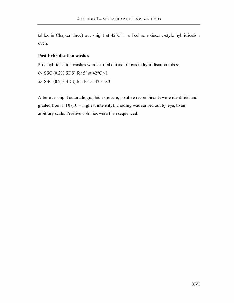
APPENDIX I – MOLECULAR BIOLOGY METHODS
tables in Chapter three) over-night at 42°C in a Techne rotisserie-style hybridisation
oven.
Post-hybridisation washes
Post-hybridisation washes were carried out as follows in hybridisation tubes:
6× SSC (0.2% SDS) for 5’ at 42°C ×1
5× SSC (0.2% SDS) for 10’ at 42°C ×3
After over-night autoradiographic exposure, positive recombinants were identified and
graded from 1-10 (10 = highest intensity). Grading was carried out by eye, to an
arbitrary scale. Positive colonies were then sequenced.
XVI

APPENDIX I – MOLECULAR BIOLOGY METHODS
I.11 Pouring and running a Polyacrylamide gel, and gel electrophoresis.
Denaturing gel electrophoresis on 6% denaturing polyacrylamide sequencing gels was
carried out to manually genotype microsatellites isolated in this study (Chapter Three).
The following details the method of polyacrylamide gel electrophoresis.
Preparation:
Prior to running the polyacrylamide gel, it was essential to ensure that the gel rig and
plates were clean. The lower plate was cleaned with a 70% Ethanol wash, then
‘Repelcoat’ was spread evenly over the plate (siliconisation to allow easy removal of
gels), and left for two mins. A final 100% ethanol wash was carried out, and the plate
rinsed with dH2O. The top plate was cleaned by addition of a few drops of NaOH to
remove grease, then wiped over. A soak in water, then rinse with dH2O was included to
remove any remaining NaOH. After 2mins a 70% Ethanol wash was carried out, and
the plates left to dry. The gel rig was assembled by placing the lower (rabbit eared)
plate into the cassette. 0.2mm spacers were placed at either edge of the plate, and the
top plate placed on top. Clamps were tightened, and gel was then prepared and applied
as follows.
All mixing of the gel was carried out on ice, and components were added in the
following order. APS was added immediately before pouring to prevent premature
polymerisation.
Polyacrylamide gels
64ml Sequagel XR
16ml Sequagel complete
640µl 10% APS
XVII
APPENDIX I – MOLECULAR BIOLOGY METHODS
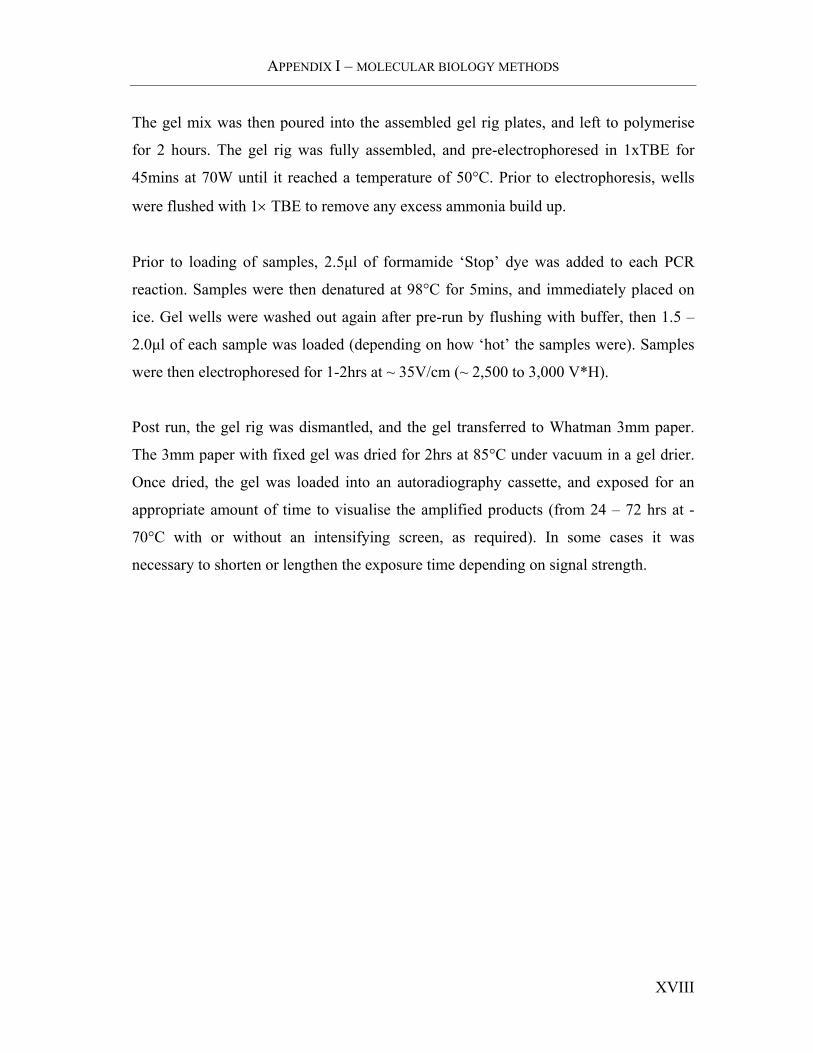
The gel mix was then poured into the assembled gel rig plates, and left to polymerise
for 2 hours. The gel rig was fully assembled, and pre-electrophoresed in 1xTBE for
45mins at 70W until it reached a temperature of 50°C. Prior to electrophoresis, wells
were flushed with 1× TBE to remove any excess ammonia build up.
Prior to loading of samples, 2.5µl of formamide ‘Stop’ dye was added to each PCR
reaction. Samples were then denatured at 98°C for 5mins, and immediately placed on
ice. Gel wells were washed out again after pre-run by flushing with buffer, then 1.5 –
2.0µl of each sample was loaded (depending on how ‘hot’ the samples were). Samples
were then electrophoresed for 1-2hrs at ~ 35V/cm (~ 2,500 to 3,000 V*H).
Post run, the gel rig was dismantled, and the gel transferred to Whatman 3mm paper.
The 3mm paper with fixed gel was dried for 2hrs at 85°C under vacuum in a gel drier.
Once dried, the gel was loaded into an autoradiography cassette, and exposed for an
appropriate amount of time to visualise the amplified products (from 24 – 72 hrs at -
70°C with or without an intensifying screen, as required). In some cases it was
necessary to shorten or lengthen the exposure time depending on signal strength.
XVIII
APPENDIX I – MOLECULAR BIOLOGY METHODS
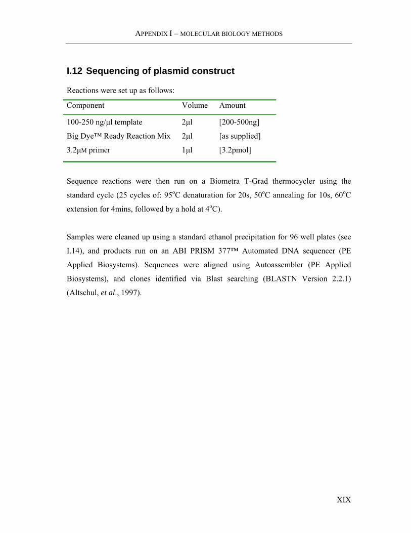
I.12 Sequencing of plasmid construct
Reactions were set up as follows:
Component Volume Amount
100-250 ng/µl template 2µl [200-500ng]
Big Dye™ Ready Reaction Mix 2µl [as supplied]
3.2µM primer 1µl [3.2pmol]
Sequence reactions were then run on a Biometra T-Grad thermocycler using the
standard cycle (25 cycles of: 95oC denaturation for 20s, 50oC annealing for 10s, 60oC
extension for 4mins, followed by a hold at 4oC).
Samples were cleaned up using a standard ethanol precipitation for 96 well plates (see
I.14), and products run on an ABI PRISM 377™ Automated DNA sequencer (PE
Applied Biosystems). Sequences were aligned using Autoassembler (PE Applied
Biosystems), and clones identified via Blast searching (BLASTN Version 2.2.1)
(Altschul, et al., 1997).
XIX

APPENDIX I – MOLECULAR BIOLOGY METHODS
I.13 Direct sequencing of PCR product
Eluent from a purified PCR product was used as a template in a direct PCR sequencing
reaction using Big Dye™ Terminator Cycle Sequencing Ready Reaction mix (PE
Applied Biosystems). Each sample was sequenced, using the appropriate forward and
reverse primer, as detailed below. The following components were added to each
sequencing reaction:
Component Volume Concentration / Amount
6-18ng/µl template 5µl [30-90ng]
Big Dye™ Diluent 2µl [2µl]
Big Dye™ Ready Reaction Mix 2µl [as supplied]
3.2µM primer 1µl [3.2pmol]
Thermal cycling was then carried out on a Biometra T-Grad using a standard cycle
sequencing cycle (30 cycles of: 95oC denaturation for 20s, 50oC annealing for 10s,
60oC extension for 4mins, followed by a hold at 4oC).
Samples were purified using a standard Ethanol / NaOAc precipitation for 96 well
plates (see I.14). Products were sequenced on an ABI PRISM 377™ Automated DNA
sequencer (PE Applied Biosystems). Post-run, gel lanes were tracked manually, and
sequence data extracted using ABI PRISM 377™ sequence analysis package version
3.4. Forward and reverse sequences were then aligned using Autoassembler (PE
Applied Biosystems) and combined to produce consensus sequences which were then
subjected to a BLAST search (BLASTN Version 2.2.1) (Altschul, et al., 1997), and
verified as the correct products.
XX

APPENDIX I – MOLECULAR BIOLOGY METHODS
I.14 Big Dye sequencing clean up method – Sanger Centre
BigDye Terminator Clean up Method.This clean-up method is good for removing excess dye from reactions, so you should
see less "dye blobs" in the sequences. The EDTA in the precipitation mix reduces the
precipitation of smaller DNA fragments and so also reduces the precipitation of un-
incorporated dye. HOWEVER, it is very important not to exceed the recommended
centrifugation time (step 3) as this will increase the dye blob problem. It is also
important to keep the precipitation mix at room temperature as both sodium acetate and
EDTA may precipitate out of the mixture if it is stored in the fridge or freezer....and
then the precipitation will not work at all!
Precipitation Mix:
100ml 96% ethanol
2ml 3M sodium acetate soln
4ml 0.1mM EDTA
Keep precipitation mix at room temperature and make up fresh solns regularly.
Protocol 96-well plates
1) For a 10µl reaction volume, add 10µl water to each well (->20µl).
2) Add 50µl pptation mix, at room temperature, to each well.
3) Spin at 4000rpm/4oC for 20-25 mins.
Note: do not exceed spin time it is not necessary to pre-chill the centrifuge
4) Tip off the supernatant, drain plates upside-down on tissue.
5) Add 100µl chilled 70% ethanol to each well.
6) Spin at 4000rpm/4oC for 2-4 mins.
n.b. for 3700 templates, repeat steps 5,6 once more.
7) Tip off the supernatant, spin plate upside-down on a tissue at 250rpm for 30-60 secs.
8) Allow plate to dry before loading.
http://www.sanger.ac.uk/Teams/Team51/BDC.shtml
XXI
APPENDIX I – MOLECULAR BIOLOGY METHODS
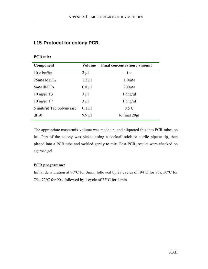
I.15 Protocol for colony PCR.
PCR mix:
Component Volume Final concentration / amount
10 × buffer 2 µl 1 ×
25mM MgCl2 1.2 µl 1.0mM
5mM dNTPs 0.8 µl 200µM
10 ng/µl T3 3 µl 1.5ng/µl
10 ng/µl T7 3 µl 1.5ng/µl
5 units/µl Taq polymerase 0.1 µl 0.5 U
dH20 9.9 µl to final 20µl
The appropriate mastermix volume was made up, and aliquoted this into PCR tubes on
ice. Part of the colony was picked using a cocktail stick or sterile pipette tip, then
placed into a PCR tube and swirled gently to mix. Post-PCR, results were checked on
agarose gel.
PCR programme:
Initial denaturation at 96°C for 3min, followed by 28 cycles of: 94°C for 70s, 50°C for
75s, 72°C for 90s, followed by 1 cycle of 72°C for 4 min
XXII
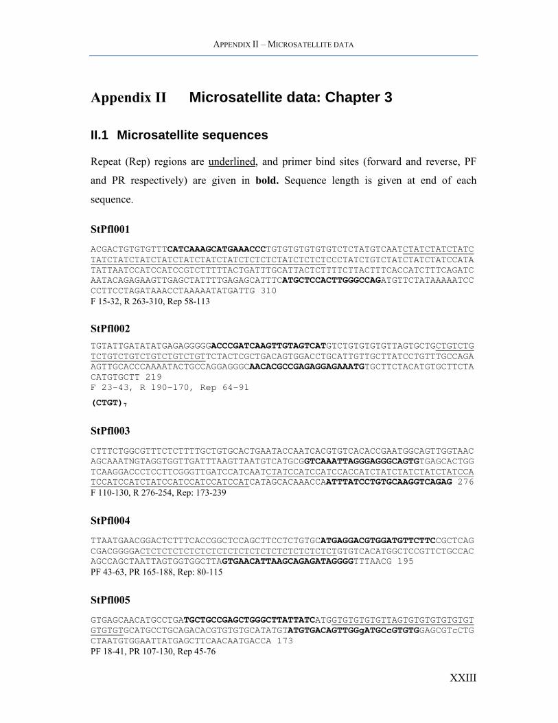
APPENDIX II – MICROSATELLITE DATA
Appendix II Microsatellite data: Chapter 3
II.1 Microsatellite sequences
Repeat (Rep) regions are underlined, and primer bind sites (forward and reverse, PF
and PR respectively) are given in bold. Sequence length is given at end of each
sequence.
StPfl001
ACGACTGTGTGTTTCATCAAAGCATGAAACCCTGTGTGTGTGTGTCTCTATGTCAATCTATCTATCTATCTATCTATCTATCTATCTATCTATCTATCTCTCTCTATCTCTCTCCCTATCTGTCTATCTATCTATCCATATATTAATCCATCCATCCGTCTTTTTACTGATTTGCATTACTCTTTTCTTACTTTCACCATCTTTCAGATCAATACAGAGAAGTTGAGCTATTTTGAGAGCATTTCATGCTCCACTTGGGCCAGATGTTCTATAAAAATCCCCTTCCTAGATAAACCTAAAAATATGATTG 310 F 15-32, R 263-310, Rep 58-113
StPfl002 TGTATTGATATATGAGAGGGGGACCCGATCAAGTTGTAGTCATGTCTGTGTGTGTTAGTGCTGCTGTCTGTCTGTCTGTCTGTCTGTCTGTTCTACTCGCTGACAGTGGACCTGCATTGTTGCTTATCCTGTTTGCCAGAAGTTGCACCCAAAATACTGCCAGGAGGGCAACACGCCGAGAGGAGAAATGTGCTTCTACATGTGCTTCTACATGTGCTT 219 F 23-43, R 190-170, Rep 64-91
(CTGT)7
StPfl003
CTTTCTGGCGTTTCTCTTTTGCTGTGCACTGAATACCAATCACGTGTCACACCGAATGGCAGTTGGTAACAGCAAATNGTAGGTGGTTGATTTAAGTTAATGTCATGCGGTCAAATTAGGGAGGGCAGTGTGAGCACTGGTCAAGGACCCTCCTTCGGGTTGATCCATCAATCTATCCATCCATCCACCATCTATCTATCTATCTATCCATCCATCCATCTATCCATCCATCCATCCATCATAGCACAAACCAATTTATCCTGTGCAAGGTCAGAG 276 F 110-130, R 276-254, Rep: 173-239
StPfl004
TTAATGAACGGACTCTTTCACCGGCTCCAGCTTCCTCTGTGCATGAGGACGTGGATGTTCTTCCGCTCAGCGACGGGGACTCTCTCTCTCTCTCTCTCTCTCTCTCTCTCTCTCTGTGTCACATGGCTCCGTTCTGCCACAGCCAGCTAATTAGTGGTGGCTTAGTGAACATTAAGCAGAGATAGGGGTTTAACG 195 PF 43-63, PR 165-188, Rep: 80-115
StPfl005
GTGAGCAACATGCCTGATGCTGCCGAGCTGGGCTTATTATCATGGTGTGTGTGTTAGTGTGTGTGTGTGTGTGTGTGCATGCCTGCAGACACGTGTGTGCATATGTATGTGACAGTTGGgATGCcGTGTGGAGCGTcCTGCTAATGTGGAATTATGAGCTTCAACAATGACCA 173 PF 18-41, PR 107-130, Rep 45-76
XXIII

APPENDIX II – MICROSATELLITE DATA
StPfl006
CTGTCATGCAAAAGAAAAGAGAGAGAGAAGAAAGGAAACAAAGAGAAACTGATTTATAAATGATGTAGATACTCCGCTATAAAAAGTATCTAGATGGATGGATAGATAAATAGTTAGATAGATAGATAGATGGATAAATAGATAGATAGATAGATAGATAGATAGATAGATAGATAGATAGATAGATAGATAGATAGATAGATAGATAGATAGATAGATAGATAGATAGATAGATAGATAGATAGATAGATAGATAGATAGATAGATGGATAGATAGATAGACACCTACCCAATGGTCCACAGACGCTGCTCAGGGGGCTGGTTATCAGGATCATCGACAGCAGCAGCATACACAGGGGAGAGGAGCTAAGGCTGAGCCCCAGGGTAGGCCTCCTGGACTGGGCCAGAGCGCCACCTGTCCTGGGCAGAGGCATGGCAGGCACCGNNTGTGGGCCGGGTCGGANATGACGGACACTCAGGTANGGCTCCACTCAACANGGATAGGCACTCTGCAGACCAGANAGANNNAAAGCATGAACGTCAG 543 PF , PR , Rep 93-280
Stpfl007
L1GCCAACAAACATCCGTTGTGAGACGAAAACAGACCAAAGGCCAAGAGTGGTGTGTGTGTGTGTGTGAGAGAGAGAGAGAGACAGACGGACAGACAGACAGACAGACAGACAGACAGACAGACAGACAGATAGACAGACAGACAGATAGACAGACAGACAGACAGACAGAGACAGACAGGTCAGAGACAGACAGGTGAGAGACAGACAGAGACAGACAGAGACAGACAGAGACAGACAGAGACAGACAGGTGAGAGACAGGTCAGAGACAGACAGGTGAGAGACAGACAGAGACTTGTTCTGGTTCTACTTTTANATCTAATCCAGGGTTACATTCTTATCCCGCTTCTGTTCTCACTTCACATCCTCGTACTTTTTGTAGNTCTGGTTCTGATTCTACTTCTAGTACCACTCCTTGTTCTGATTTTCTTTCTGCTGCTGTTGCTGGT 447bp PF 30-49, PR 352-331, Rep: 41-292
Stpfl008
CGGCGCTCGGGGAGCAGATGTCTGGGGAGTAAGGTGCCTTGCTCAGGGGCACTAGACAGGGTAGGGAGACTCTTGGATTTTTGGACAGATCAATCCAGGTTATTCTTTTGTTGTCTCTCCGTGGAGTCGAACCAGAGACGAACCAGAGACCTTCTCTGCCCATANTCCAAGTTTCTATAGATAGATAGATAGATAGATAGATAGATAGATGGATGGATAGAAATAAAGATAGAgATGGATGGATATATGGATGGATGGATAAGGGTGAAAACTCAGTTGTATATGTGTCTATCCCTTTAAGACTCCATTAAAATAAATAAAATACTTtACTTATCTNATCTCCCCCCACATGTCATCTTATTAAACTTTCCAGNCTCAACATTTCTGTCTCAAATCTGTCCCCTGTATNCANTCATCATCACCCATGCTCA 431bp PF 129-151, PR 406-383, Rep:180-260
Stpfl009 CTGCTCAATGCCTTGATCATTTTAAGAAGGAATCTTTGAGACAnGGAGGAGTTTTCTTTGTTTTAGCACAACATGAAACTTGTAAAGtaCAAGTTAGATAgATAGATAGATAGATAGATAGATAGATAGATAGATAGATAGaCAGATAGATAGATAGAGAGATAGATAGATAGATAGATAGATATAGATGGATCGATGGATAGATAGACAGATAGATaGATaGATAGATAGATAGATaGATaGATAGATAGATAGATAGATAGATAGATAGATagATAGATTGATaGAAGCAcTTGtTAGATCACTAaTaATATAGTCATAACACTGACmAACCATaATATTGCATCAATAAAGAATTAGAACATTACATTGCCTTGCATTACTATTAAACAATTACATTGtAaCACCAGTAATAAGCAATTCTGGCTTAAATGCTGTATTTyGAAATGCTTGACTTGACaAGATGTCCCACTGTCCTGTCACCAAAGGGAGCCGGGTGACAGCCAAwAAGTACAAGTCmaTTTAAATGCTGTTAACCAACCCCAAAAGGCTCTTAGCcAAAGCATTGAATGG PF 45-66, PR 330-306, Repeat: 98-287
StPfl010
ACTGTTGCTTGTNGCATTTATATCTATGTTTACAGGGTCATGCAAAAATGATGTTGTTTATGTGGTTCTCTTAACAAATCCCTAAGTGTTCTTTATAGAAACTGATCCAAACAAAGCGCAGTGCTTCACCTTGTTTTTGCTCTCATTGGGGTGACCTATCTACCTGTCTGTCTGTCTGTCTGTCTGTCTGTCTGTCTGTCGGTCTGTCTG
XXIV
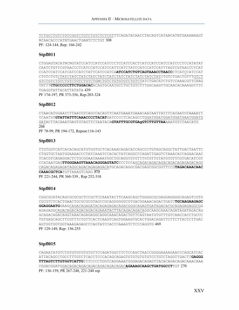
APPENDIX II – MICROSATELLITE DATA
TCTGCCTGTCTGTCGGTCTGTCTGTCTCTCGTTTCAGATACAACCTACAGTCATANCATNTGAAANAAGTNCAACACCCATNTGAACTGANTCTCTGT 308 PF: 124-144, Rep: 166-242
Stpfl011
CTGGAGTACATNCNGTATCCATCCATCCATCCCTCCATCCACTCATCCATCCATCCATCCCTCCATATATCAATCTGTTCGTAACCCTCATCCATCCATCCATTCATCTATCCATCCATCCATTTAGTCGTAACCCTCATCCATCCATCCATCATCCATCTATTCATCCATCAATCCATCTGTCAGTAAACCTAACCCTCATCCATCCATCTGTCTGTCTATCTATCTATCTATCTATCTATCTATCTATCTATCTATCTATCTGTCTGACTGTTTGTCTGTCTGTCTGTCTGTCTGTCTGTCTGNCTGTCTGTGTGTCTGTCTATCTGACATCTGTCCAAACGTTCAAGTNTTTCTGCCCCCTTCTGGACACACAGTGCAATGCCTGCTGTCTTTGGCAAGTTGCAACACAAAGGTTTCTGAGGTATTACATTATATA 439 PF 174-197, PR 373-356, Rep:203-324
Stpfl012
CTAACATGGAATCTTAATGTCAGCCACAGTTCAATGAAATGAAACAATAATTATTTCATAATGTAAAATTTCAATGTGTATTATTTCAAACCCCTACATGATCCCCTCACAGCCTGGATGGATGGATGGATGAATGGATGGATACTTACAAATGAGTGTAGTTCTAATACAGTATTTGCGTGAgGTCTTGTTAAAAATGTCTAACATG 208 PF 78-99, PR 194-172, Repeat:116-143
Stpfl013
TTGTGGTCATCACACAGCATGTGGTGCTCACAAACAGACACCAGCCCTGTAGCAGGCTATTGACTAATTCCTGGTGCTAATGGAAAACCCTATCAAATCCACACTATCAGGCCCAGATTGAGTCTAAACACCAGAACAACTCACGTCAGAGGACTCTGCGGAATAAAATGGCTGCAGGTGTGTTTGTGTTGTATGTGTTCGTGACATCGTCCATAATGAGTTGGGAAGTTAAACAGGGAGTATCTCCTCCAGCAGACAGACAGACAGACAGAGAGACAGGCAGACAGAGAGATAGGCAGACAGAGAGACATGCAGACAGGCGACGAGCGGCGGTTCCGTAGACAAACAACCAAACGCTCATGTTAAAGTCAAG 373 PF 221-244, PR 360-339 , Rep 252-310
Stpfl014
CGGCGCATACAGCGCGCGCTCCGCTCCAAATACTTCAAGCAGCTGGGGCGCGAGGAGGGGCAGAGTCGTGCGCGTCTCACTGAACTGCGCGCGTAGCCGCAGGGGGGCGTGACGGAAACAGACTGATCTGCAAGAAGAGCGGAGGAATGGAAGCAGACAGAGATACAGAGAGACAGACGGGCAGAGTGATAGACACGCAGAGAGAGGCGGAGAGAGGCAGACAGACAGACAGACAGAAATACTTACAGACAGACAGGCAAGCAAACAGATAGATAGACAGGCAGACAGACAGGTAAACAGAGAGGCAGGCAAACAGACTGTTCAGTAATGTGTTTGTCAACCACCTGCCCTGTGAGCAGCTTCGTTTCTGTTCACTCAAGTCAGTGGAAGTGCACTGGACAGATTCTTCTTACTCTTGACAGTGGTGGTGGTAAAGAGAGCCCAGTATCCACCCAAAGTCTCCCAGGTG 469 PF 129-149, Rep: 156-255
Stpfl015
CAGAATATGTCTGTGTGTGTGTGTTCCAGATGGCTTCTCCAGCTAACCGGGGAAAAGAACCCAGCATCACATTACAGCCTGCCTTTGTCTCACCTCCCACAGCAGAGTGTGTGTGTGTCCTGTCTAGGTTGACTTGAGGGTTTAGTCTTGTGGTCATTGTTTCCCCTGGTCAGGAAATGGGAGACAGAGTTACACAGACAGACAAACAAACGGACGGATGGACAGACAGACAGACAGACAGACAGACAGAAAGCAAGCTGATGGCCTTGT 270 PF: 136-159, PR 267-248, 221-248 rep
XXV
APPENDIX II – MICROSATELLITE DATA
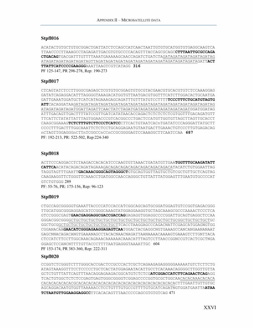
Stpfl016
ACATACTGTGCTGTGCGGACTGATTATCTCCAGCCATCAACTAATTGTGTGCATGGTGTGAGGCAAGTCATTAACCCCTTAAAGCCTAGAGATTGACGTGTGCCCCACAGTTTACCAGCGCAGCCTTTAATTGCGCCAGACTGACAGTGACGATTTGTTTTAAATGAAAAAGCAACCAGATCTGATCTAGATAGATAGATAGATAGATAGATAGATAGATAGATAGATAGTTAGATAGATAGATAGATAGATAGATAGATAGATAGATAGATAGATTACTTTATTCATCCCCGAAGGGAAATTAAGTCGTCATAGG 316 PF 125-147, PR 298-278, Rep: 190-273
Stpfl017
CTCAGTATCTCCTTGGGCGAGAGCTCGTGTGCGGAGTGTGCGTACGAACGTGCACGTGTCTCCAAAGGAGGATATCAGAGGACATTTAGGGGTAAAGACATGGTGTTAATGACGTGGTTTCATCTTGGACACTGCAATGAGATTGAAATGGATGCTCATCATAGAAAGAGCAGATTTGTTTATGTCCTTTTTCCCTTTCTGCATGTAGTGATTCACAGGATAAGATAGATAGATAGATAGATAGATAGATAGATAGATAGATAGATAGATAGATAGATAGATAGATAGATAGATGGATTAGATTCAACTATCTAGATGATAGATAGATAGATAGATAGATGGATGGATAGATTTGACAGTTGACTTTTATCCGTTGATCATATAACACCAGACTCTCTCTCTCGTGGTTTGACAGATGTTTTCATTCTATATTATTTAGTGGAACCCGTCACGGCCCTGACTCCATGTTGGTGTTAGCTTAGTTGCACCTCAAGCGGAAAGTCTCTTTGTCTTCCCTCATCCCTTCACTGTAATCACnTGATATCCCAGGGATTATGCTTCCCCTTTGACTTTGGCAAATTCTCTCCTGCAGGAGAATGTAATGACTTGAAACTGTCCCTTGTGAGACAGnCTAGTTGGAGGGnCTTnTCGGCCnCCnCCGCGGGGAGTCCAAAGGCTTCAATCCAA 687 PF: 192-213, PR: 522-502, Rep:224-340
Stpfl018
ACTTCCCAGGACCTCTAAGACCACACATCCCAAGTGTTAAACTGATATGTTGAATGGTTTGCAAGATATTCATTCAACATACAGACAGATAGAAAGACAGACAGACAGACAGACAGACAGACATACATCTGTGGAATTAGTAGGTAGTTTGAATTGACAAACGGGCAGTAGGGCTGTGCAGTGGTTAGTGCTGTCGCTGTTGCTCAGTAGCAAGAAGGTTCTGGGTTCAAACCTGATGGCCAACCAGGGCTGTTATTTATGGAGTTTGAATGTGCCCCATGTCTGTGGG 289 PF: 55-76, PR: 175-156, Rep: 96-123
Stpfl019
CTGCCAGCGGGGGTGAAATTACCCCATCCACCATCGGCAGCAGTGCGGATGGAGTGTCCGGTGAGACGGGTTGCATGGCGGGAGGAGCATCCGGGCAAAGTATGGAGGAAGGTGCTAGCAAAGCGCCCAAAACTCCCTCAGTCCGGGCGAGTGAACGAGGAGGCGACCGACCAGGAGAGGTGGAGGCCCCGGATTGCAGTGAGGCTCCAAGGGACGGCGGGGCTGCTGCTGCTGCTGCTGCTGCTGCTGCTGCTGCTGCTGCTGCGGCTGCTGCTGCTGCGGCTGCGGCTGCTGCTGCTGCTGCTGCTGCTTCACCTAAGGAGCCCAGACNATTCGAGCATGGAGNGTGGCGGANACAAGAACATCGGGAGAAGGAGAGTCAATGGACTACGAGGCNGTGAAAGCCANCANGAANANAATGAGCNNACAGACANGTGAAANAGCCTACACNAACNAGATTAANAAAACAAAAGTGAAAGTCTTGNTTACACTCCATCTTCCTTGGCAAACAGAAACAAAAAACAAACATTTAGTCCTTAACCGGNCCGTCACTCGCTNGAGGAGCTCCANCNTTTTGTTACCCTTTTAATGAGGGTAAAATTGC 604 PF 153-174, PR 383-360, Rep: 222-311
Stpfl020 CCGGTCTCGGGTCTTTGGGCACCGACTCCGCCCACTCGCTCAGAAGAGAGGGGGAAAAATGTCTCTTCTGATAGTAAAGGTTTCCTCCCCCTGCTCACTATGGAGAATACATTGCCTCACAAACAGGGGCTTGGTTGTTAGCTCTGTTTATTCAGTTTAACAGGAGAAGACGGCATGTCTCTCGATCGGACCATCTTCAGAACTCAGAGGTCACTGTGGCTCTCTCCGAGTGAGTGGGCGGGGTCGGAGCCCCGGTGCGCTGGCAACACACAAACACACACACACACACACACGCACACACACACACACACACACACACACACACACACACACACTTTGAATTGTTGTGCAGCAGGACAATGTGGTTAAAAACCTCCTGTTTGTGCCGTTTTGTGCATCAGATNGTGGATGAATTAATAATCTAATGTTGGAAGGAGGCCTTCACACAGTTTAACCCCCAGCGTGTGTCAG 471
XXVI
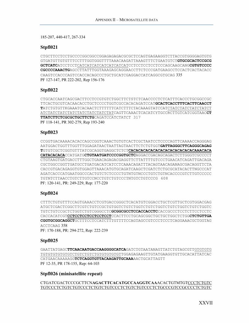
APPENDIX II – MICROSATELLITE DATA
185-207, 440-417, 267-334
Stpfl021
CTGCTTCCTCCTGCCCCGGCGGCCGGAGAGAGACGCGCTCCAGTGAGAAGGTCTTACCGTGGGGAGTGTGGTGATGTTGTGTTTCCTTTGGTGGGTTTTAAACAAGATTAAAGTTTCTGAATGTCTGTGCGCACTCCGCGGCTCATCATCCTCCTCATCATCATCATCATCATCATCCTCCTCCTCCTCCCAGCAAGCANGCGTGTCCCCCGCCCCAAACTGAGCCTTATTTGGTAAAGAGCAGGAACCTTCTCCCGATGAAGCCTCCACTCACTACACCCAAGTCCACCCAGTCCACCACAGCCCTGCTGCATCGAGGACCATCAGGCGTGCAG 335 PF 127-147, PR 222-202, Rep 156-176
Stpfl022
CTGCACCAATCAGCGACTTCCTCCGTGTCTGGCTTCTSTCTCAACCCCTCTCATTTCACCCTGCGGCCGCTTCACTGCGTCACAACACCTGCTCCCCTGGTCGCCACACAGATCCATGCACTCACCTTTCACTTCAACCTTATCTGTGTTKGAAATCACAACTCTTTTTTCATCTTTCTACAAAGTATCCATCTATCTATCTATCTATCTATCTATCTATCTATCTATCTATCTATCTATCAGTTCAAACTCACATCYTGCCRCTTGTCATCGGTAACCTTTATCTTCTCGCGCTGCTTCTGCAGATCCATCTATCT 317 PF 118-141, PR 302-279, Rep 193-240
Stpfl023
CCGGTGACAAAACACACCAGCCGGTCAAACTGTGTCACTCGCTAATCCTCCCCAGTTCAAAACCAGGGAGAATGGACTGGTTTGGTTTGGAGATAACTAATTAGTAACTTCTCTGTGGTGATTAGGGCTTCAGGGCAGAGTGTGTCGCTCGGTGTTTATCGCAGGTGAGGCTCTCTCACACACACACACACACACACACACACAAACACACATACACACACCATGATGCTGTAATGATCCCCGGTGCTCAGGACCGACAGCAGACTCTTGGGTCGCCCCTCTGTAAGTGATGACCTTTGGCTGAACAGAGACGAGGTTCTTATTTTGTCCCTGAACATCAGATTGACAGACGCTGGCCGGTTGATGCCTGATGACATCATCCTCAAACAGATTTACAGTAACAGANAGCGACAGGTTCTACACCGTGACAGAGGTGTGGAGTTAAACATGTGCAGATCAAGCTCGATCTCTGCGCATACACTTNGCCCATAGATCACCCATGAATGGCCCACTGTCTCTCCCCTGTNTGTNCCCTGTCTGTNCACCCCGTCTTGTCCCCCTGTNTCTTAACCTGTCTTGTCCNCCTGTCTGTCCCTNTGTCTGTCCCG 608 PF: 120-141, PR: 249-229, Rep: 177-220
Stpfl024
CTTTCTGTGTTTCCAGTGAAACCTCGTGACCGGGCTCACATGTCGGACCTGCTCGTTGCTCGTGGACGAGATGCTCGACTCGGCTTCGTCTGTCCGCTGTGGTCTGTCTGGTCTGTCTGGTCTGTCTGGTCTGTCTGGTCTGTCTGTCCGCTCTGGTCTGTCGGGCCTCGCGGCGCCTCCACCACCTCCACCGCCCTCCTCTTCCTCCTCCACCACATCGTCCTCCTCCTCCTCCTCCTCCACTTCCTGCAGCGGCTGCTGCTGGCTCTGGCTCTGTTGACGGTGCGGCAGGCTGCTTTCCTCCATCTTTGTTTTCCAGTAGCCGTCCCTCCCTCAGGAAACGCTGGTAGACCTCAAG 358 PF: 170-188, PR: 294-272, Rep: 222-239
Stpfl025
GAATTATGAGCTTCAACAATGACCAAGGGGCATCAGATCTGTAATANAGTTATCTGTAGCGTTGTGTGTGTGTGTGTGTGTGTCTGTCTGTCTGTGTGTGTGTTGGAGAGAAGTTGTATGAAGGTGTTGCACATTATCACCATGAACAAAAAGGTCTCAGGTGTTACAAGATTGCAAAAACTGCATTAGTT PF 12-35, PR 178-155, Rep: 64-103
Stpfl026 (minisatellite repeat)
CTGATCGACTCCCGCTTCNAGACTTCACATGCCAAGGTCAAACACTGTMTGTCCCTCTGTCTGTCCCTCTGTCTGTCCCTCTGTCTGTCCCTCTGTCTGTCCCTCTGCCCGTCCGCCCCTCTGTC
XXVII

APPENDIX II – MICROSATELLITE DATA
TGTCACTCTGTCTGTCCGTCCCTCTGTCTGTCTCTCTCTGCTTGTCCCTCTGCCCGTCCGCCCCTCTGTCTGTCCCTCTGTCGGCCTGTCCCTCTGTCCGTCTGTCCCTCTGTCTGTCTCTCTGTCTGTCCGTCCCTCTGTCCGTCTGTCTGTCCCTCTGTCTGTCCCTCTGTCTGTCCCTCTCTGCTTGTCCCTCTGTCTGTCTGTCCCTCTGTCTGTCCCTCTGTCTGTCCCTCTGTCTGTCTGTCTGTCCCTGATGGTTCTAACGTCTCTCTACCTCAGGGTTCTCTGAGCGTCTCTMAG 428 PF 20-41, PR 417-396 Rep 53-374
Non-Enriched libraray
Stpfl027
CTGACTGGACGTCTCTCTGAGCATGAACCTGGTGACGAACTGACCCAACACACTGGAGCCCTGGTACTCCTGAGGGAGAGAGAGAGAGAGAGAGAGAGAGAGAGAGAGAGAGAAACAAAGAAGCAGATGTCAAAGCCCGAACTGAAGCAACGGCAAAGTAAAAGCATCTCAGGGACAAAACAGAAGGGAAAGATAACTTTGAATAACTTTCAACCAAAACAAATATTCCAGGCACCTTTGTGATGTGTCAGCCGGTATGAAACCCTACTAATTAATTYTCTTGACACCCACATGTATAATTCATTAGTACAAATCCAAATTCCAAGGTGAAGGAGCTCAGCGGGGCATCCCTCATGACTGAGGGCCCTCGTCTGTGTGGTAACGACTGGGTTTTTCAGCAGGACAACGGCTCCAACTTCACAATGCCCGTCTGACCAAGACTTTTTTCCAGGAGAATAACATCACTCTTTTGGACCATCCTGCGTGTTCCCCTAATCTTAATCCAATTGAGAACATTTGGGGATGGATGGCAAGGGAATTTTACAAAAATGGACTTCAGTTCCAGACAGTGGATGCCCTTCATGAAGCCATCTTCACCACTTGGCGCAACATTCGCACTAGCCnTTTTGGAAACACTTGCATYAAGCATGCCAAAACGAATTTTTTGATGTGATCAACMATAATGGTGGAGA 692 PF: 31-52, PR: 143-122, Rep: 76-113
Stpfl028
CTGCTCCTCACAAAGAGAGACACACACACACACACACACACTCAATACCAACACCAGCACCATCCTGGCCTTCGCTTCCAATTTGATGAATTTTTCCATTTGAGTTCTTTTAAAAATTCATCCAGTGAGAAAAATCTTGTTTTTTGTGACCCGACTGCTGGAGGGAGGAGGGAAATGAGAGCGGTCTTCTGTGRAGTTGGACCGGAGGAACTCGCTTTTTAAAGCGCGGCTCTTTGYTCCCACATGCAGCGCCATGGGACACGTGTGTGTCTGTGTGTGTTTGTGTGTCTGTGTGTGAGTGTCTTACAGATGTATATGTTCATGTCAGCAGGCATCTTGAGTCGG 345 PF 201-224, PR: 336-313 Rep 263-296
Stpfl029
CTWCGTCTTCTSKCTACTAACACATTTTAnCAGGTGTGYATCACATCAATGTTCCTTTATCTAGCAACACCTCAATGTnTAGTGWCATTGYTCCAATTGTGWGATAGTAGAGCCSAGAGWTAGAGAKTASATAGAGTAAnGAGAGAGAGAGAGAGAGACATTGCAAGACATAAAGATTCCTTTGATCTAGGACCACTGACAATGTCACTGCAGGAGTGGAGTTGTTTGTGTGACATAAAATCGATCCCTGAGTCAGTTTTTATCTCCCATCTTGCTGAGATGACACTCATCTCAATTTGAAG 302PF: 56-77, PR: 194-173 Rep 141-158
XXVIII
APPENDIX II – MICROSATELLITE DATA
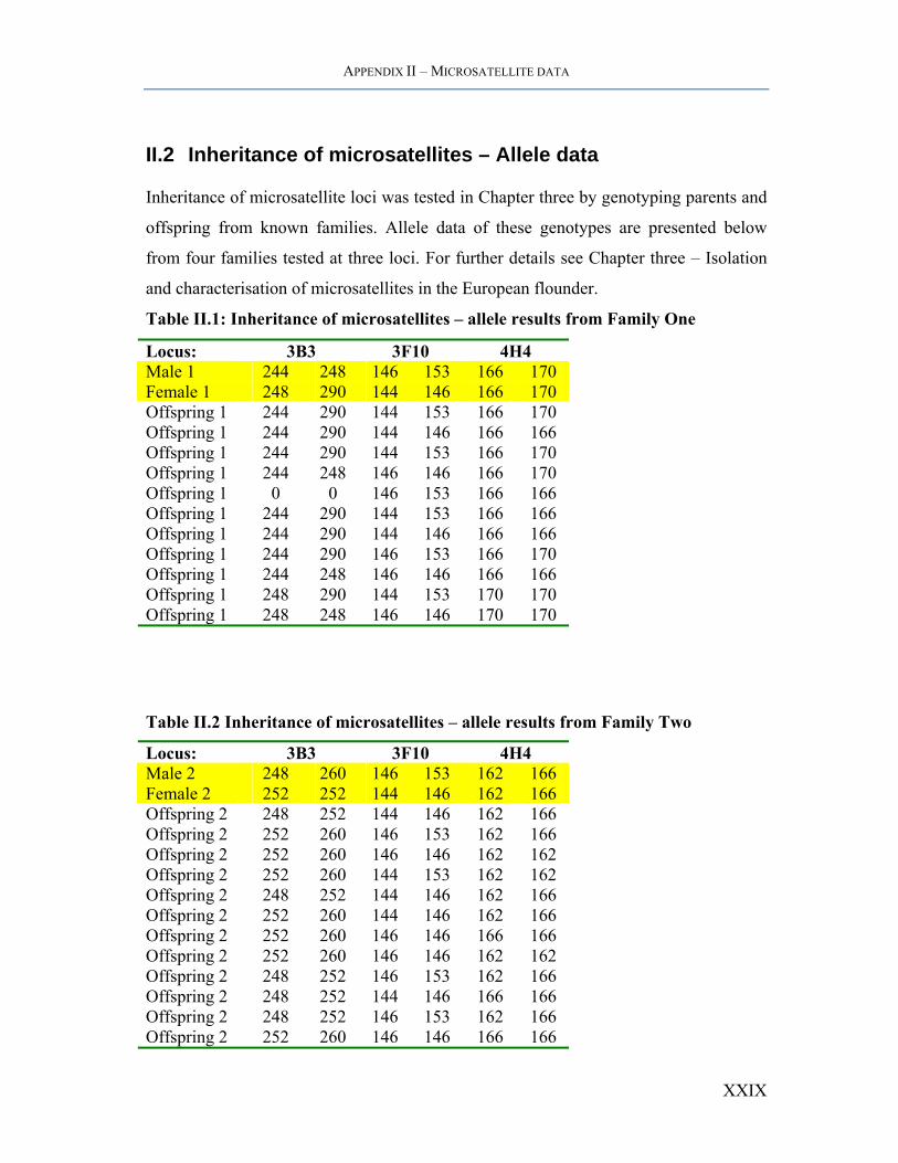
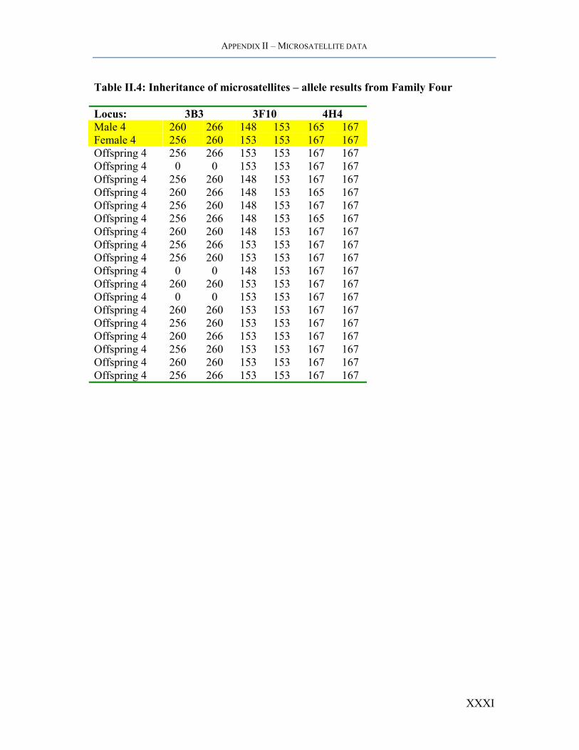
II.2 Inheritance of microsatellites – Allele data
Inheritance of microsatellite loci was tested in Chapter three by genotyping parents and
offspring from known families. Allele data of these genotypes are presented below
from four families tested at three loci. For further details see Chapter three – Isolation
and characterisation of microsatellites in the European flounder.
Table II.1: Inheritance of microsatellites – allele results from Family One
Locus: 3B3 3F10 4H4 Male 1 244 248 146 153 166 170 Female 1 248 290 144 146 166 170 Offspring 1 244 290 144 153 166 170 Offspring 1 244 290 144 146 166 166 Offspring 1 244 290 144 153 166 170 Offspring 1 244 248 146 146 166 170 Offspring 1 0 0 146 153 166 166 Offspring 1 244 290 144 153 166 166 Offspring 1 244 290 144 146 166 166 Offspring 1 244 290 146 153 166 170 Offspring 1 244 248 146 146 166 166 Offspring 1 248 290 144 153 170 170 Offspring 1 248 248 146 146 170 170
Table II.2 Inheritance of microsatellites – allele results from Family Two
Locus: 3B3 3F10 4H4 Male 2 248 260 146 153 162 166 Female 2 252 252 144 146 162 166 Offspring 2 248 252 144 146 162 166 Offspring 2 252 260 146 153 162 166 Offspring 2 252 260 146 146 162 162 Offspring 2 252 260 144 153 162 162 Offspring 2 248 252 144 146 162 166 Offspring 2 252 260 144 146 162 166 Offspring 2 252 260 146 146 166 166 Offspring 2 252 260 146 146 162 162 Offspring 2 248 252 146 153 162 166 Offspring 2 248 252 144 146 166 166 Offspring 2 248 252 146 153 162 166 Offspring 2 252 260 146 146 166 166
XXIX

APPENDIX II – MICROSATELLITE DATA
Table II.3: Inheritance of microsatellites – allele results from Family Three
Locus: 3B3 3F10 4H4 Male 3 248 253 146 148 167 167 Female 3 248 260 144 153 165 167 Offspring 3 252 260 146 153 167 167 Offspring 3 253 261 144 148 167 167 Offspring 3 248 260 144 146 167 167 Offspring 3 248 260 144 146 167 167 Offspring 3 248 248 146 153 167 167 Offspring 3 253 260 146 153 167 167 Offspring 3 248 248 148 153 167 167 Offspring 3 248 260 144 146 167 167 Offspring 3 248 253 146 153 167 167 Offspring 3 248 248 146 153 165 167 Offspring 3 248 248 144 146 165 167 Offspring 3 248 260 148 153 167 167 Offspring 3 248 253 144 148 167 167 Offspring 3 248 253 148 153 167 167 Offspring 3 0 0 0 0 0 0 Offspring 3 248 260 148 153 167 167 Offspring 3 248 253 146 153 167 167 Offspring 3 248 260 148 153 167 167
XXX
APPENDIX II – MICROSATELLITE DATA
Table II.4: Inheritance of microsatellites – allele results from Family Four
Locus: 3B3 3F10 4H4 Male 4 260 266 148 153 165 167 Female 4 256 260 153 153 167 167 Offspring 4 256 266 153 153 167 167 Offspring 4 0 0 153 153 167 167 Offspring 4 256 260 148 153 167 167 Offspring 4 260 266 148 153 165 167 Offspring 4 256 260 148 153 167 167 Offspring 4 256 266 148 153 165 167 Offspring 4 260 260 148 153 167 167 Offspring 4 256 266 153 153 167 167 Offspring 4 256 260 153 153 167 167 Offspring 4 0 0 148 153 167 167 Offspring 4 260 260 153 153 167 167 Offspring 4 0 0 153 153 167 167 Offspring 4 260 260 153 153 167 167 Offspring 4 256 260 153 153 167 167 Offspring 4 260 266 153 153 167 167 Offspring 4 256 260 153 153 167 167 Offspring 4 260 260 153 153 167 167 Offspring 4 256 266 153 153 167 167
XXXI
APPENDIX III – FLOUNDER CYP1A
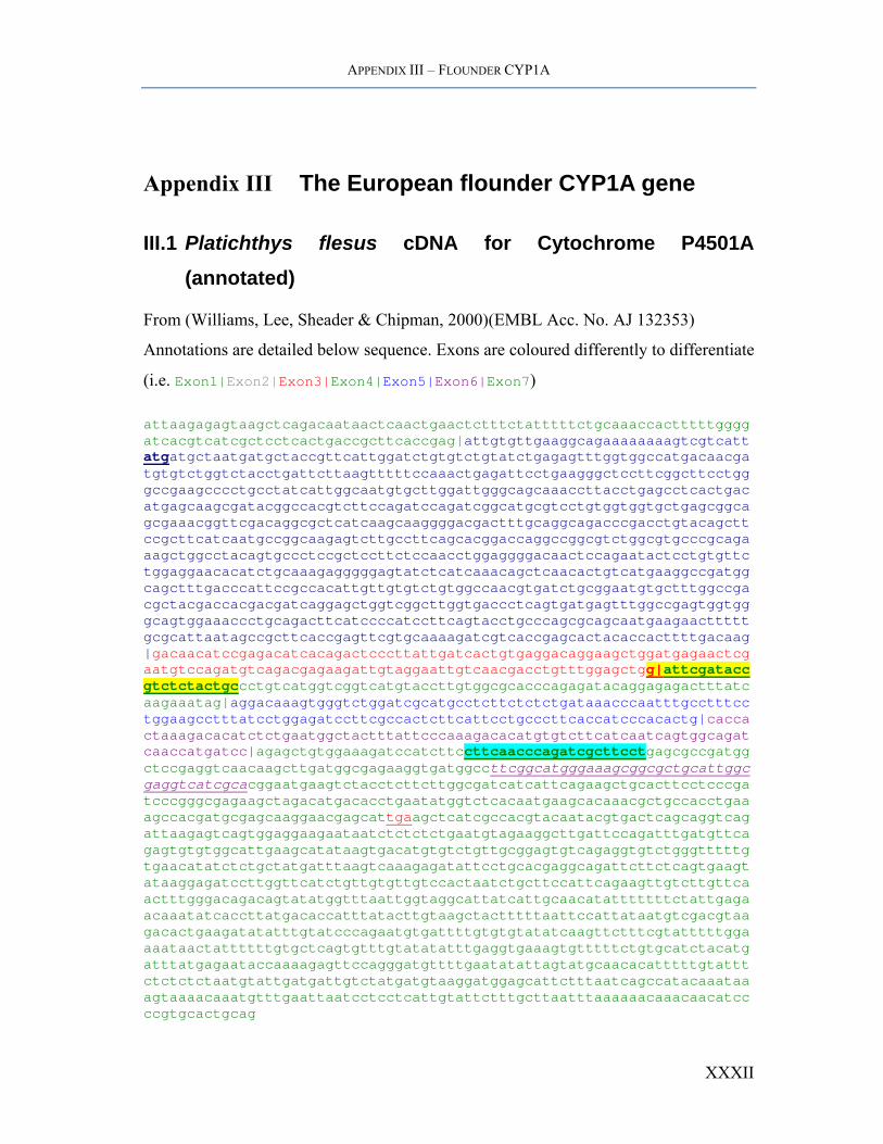
Appendix III The European flounder CYP1A gene
III.1 Platichthys flesus cDNA for Cytochrome P4501A (annotated)
From (Williams, Lee, Sheader & Chipman, 2000)(EMBL Acc. No. AJ 132353)
Annotations are detailed below sequence. Exons are coloured differently to differentiate
(i.e. Exon1|Exon2|Exon3|Exon4|Exon5|Exon6|Exon7) attaagagagtaagctcagacaataactcaactgaactctttctatttttctgcaaaccactttttggggatcacgtcatcgctcctcactgaccgcttcaccgag|attgtgttgaaggcagaaaaaaaagtcgtcattatgatgctaatgatgctaccgttcattggatctgtgtctgtatctgagagtttggtggccatgacaacgatgtgtctggtctacctgattcttaagtttttccaaactgagattcctgaagggctccttcggcttcctgggccgaagcccctgcctatcattggcaatgtgcttggattgggcagcaaaccttacctgagcctcactgacatgagcaagcgatacggccacgtcttccagatccagatcggcatgcgtcctgtggtggtgctgagcggcagcgaaacggttcgacaggcgctcatcaagcaaggggacgactttgcaggcagacccgacctgtacagcttccgcttcatcaatgccggcaagagtcttgccttcagcacggaccaggccggcgtctggcgtgcccgcagaaagctggcctacagtgccctccgctccttctccaacctggaggggacaactccagaatactcctgtgttctggaggaacacatctgcaaagagggggagtatctcatcaaacagctcaacactgtcatgaaggccgatggcagctttgacccattccgccacattgttgtgtctgtggccaacgtgatctgcggaatgtgctttggccgacgctacgaccacgacgatcaggagctggtcggcttggtgaccctcagtgatgagtttggccgagtggtgggcagtggaaaccctgcagacttcatccccatccttcagtacctgcccagcgcagcaatgaagaactttttgcgcattaatagccgcttcaccgagttcgtgcaaaagatcgtcaccgagcactacaccacttttgacaag|gacaacatccgagacatcacagactcccttattgatcactgtgaggacaggaagctggatgagaactcgaatgtccagatgtcagacgagaagattgtaggaattgtcaacgacctgtttggagctgg|attcgataccgtctctactgccctgtcatggtcggtcatgtaccttgtggcgcacccagagatacaggagagactttatcaagaaatag|aggacaaagtgggtctggatcgcatgcctcttctctctgataaacccaatttgcctttcctggaagcctttatcctggagatccttcgccactcttcattcctgcccttcaccatcccacactg|caccactaaagacacatctctgaatggctactttattcccaaagacacatgtgtcttcatcaatcagtggcagatcaaccatgatcc|agagctgtggaaagatccatcttccttcaacccagatcgcttcctgagcgccgatggctccgaggtcaacaagcttgatggcgagaaggtgatggccttcggcatgggaaagcggcgctgcattggcgaggtcatcgcacggaatgaagtctacctcttcttggcgatcatcattcagaagctgcacttcctcccgatcccgggcgagaagctagacatgacacctgaatatggtctcacaatgaagcacaaacgctgccacctgaaagccacgatgcgagcaaggaacgagcattgaagctcatcgccacgtacaatacgtgactcagcaggtcagattaagagtcagtggaggaagaataatctctctctgaatgtagaaggcttgattccagatttgatgttcagagtgtgtggcattgaagcatataagtgacatgtgtctgttgcggagtgtcagaggtgtctgggtttttgtgaacatatctctgctatgatttaagtcaaagagatattcctgcacgaggcagattcttctcagtgaagtataaggagatccttggttcatctgttgtgttgtccactaatctgcttccattcagaagttgtcttgttcaactttgggacagacagtatatggtttaattggtaggcattatcattgcaacatatttttttctattgagaacaaatatcaccttatgacaccatttatacttgtaagctactttttaattccattataatgtcgacgtaagacactgaagatatatttgtatcccagaatgtgattttgtgtgtatatcaagttctttcgtatttttggaaaataactattttttgtgctcagtgtttgtatatatttgaggtgaaagtgtttttctgtgcatctacatgatttatgagaataccaaaagagttccagggatgttttgaatatattagtatgcaacacatttttgtatttctctctctaatgtattgatgattgtctatgatgtaaggatggagcattctttaatcagccatacaaataaagtaaaacaaatgtttgaattaatcctcctcattgtattctttgcttaatttaaaaaacaaacaacatccccgtgcactgcag
XXXII
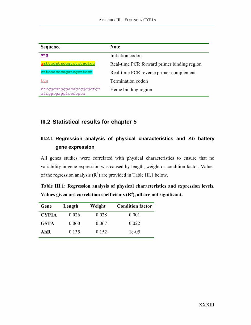
APPENDIX III – FLOUNDER CYP1A
Sequence Note atg Initiation codon gattcgataccgtctctactgc Real-time PCR forward primer binding region cttcaacccagatcgcttcct Real-time PCR reverse primer complement tga Termination codon ttcggcatgggaaagcggcgctgc attggcgaggtcatcgca
Heme binding region
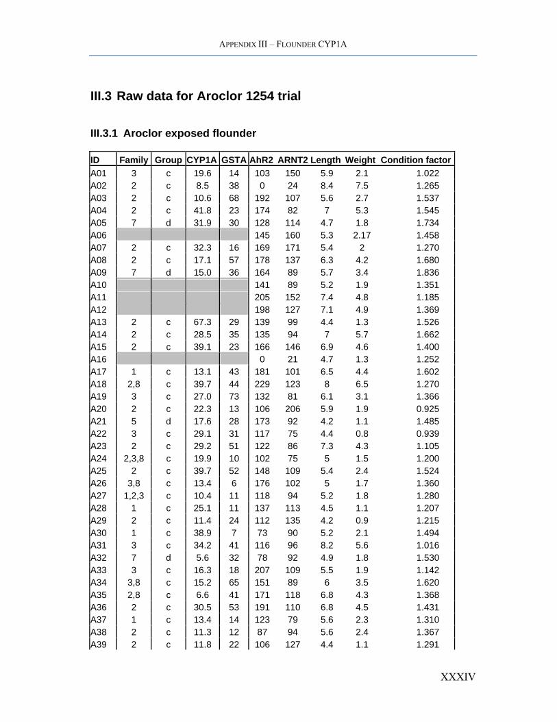
III.2 Statistical results for chapter 5
III.2.1 Regression analysis of physical characteristics and Ah battery gene expression
All genes studies were correlated with physical characteristics to ensure that no
variability in gene expression was caused by length, weight or condition factor. Values
of the regression analysis (R2) are provided in Table III.1 below.
Table III.1: Regression analysis of physical characteristics and expression levels.
Values given are correlation coefficients (R2), all are not significant.
Gene Length Weight Condition factor
CYP1A 0.026 0.028 0.001
GSTA 0.060 0.067 0.022
AhR 0.135 0.152 1e-05
XXXIII
APPENDIX III – FLOUNDER CYP1A
III.3 Raw data for Aroclor 1254 trial
III.3.1 Aroclor exposed flounder
ID Family Group CYP1A GSTA AhR2 ARNT2 Length Weight Condition factorA01 3 c 19.6 14 103 150 5.9 2.1 1.022 A02 2 c 8.5 38 0 24 8.4 7.5 1.265 A03 2 c 10.6 68 192 107 5.6 2.7 1.537 A04 2 c 41.8 23 174 82 7 5.3 1.545 A05 7 d 31.9 30 128 114 4.7 1.8 1.734 A06 145 160 5.3 2.17 1.458 A07 2 c 32.3 16 169 171 5.4 2 1.270 A08 2 c 17.1 57 178 137 6.3 4.2 1.680 A09 7 d 15.0 36 164 89 5.7 3.4 1.836 A10 141 89 5.2 1.9 1.351 A11 205 152 7.4 4.8 1.185 A12 198 127 7.1 4.9 1.369 A13 2 c 67.3 29 139 99 4.4 1.3 1.526 A14 2 c 28.5 35 135 94 7 5.7 1.662 A15 2 c 39.1 23 166 146 6.9 4.6 1.400 A16 0 21 4.7 1.3 1.252 A17 1 c 13.1 43 181 101 6.5 4.4 1.602 A18 2,8 c 39.7 44 229 123 8 6.5 1.270 A19 3 c 27.0 73 132 81 6.1 3.1 1.366 A20 2 c 22.3 13 106 206 5.9 1.9 0.925 A21 5 d 17.6 28 173 92 4.2 1.1 1.485 A22 3 c 29.1 31 117 75 4.4 0.8 0.939 A23 2 c 29.2 51 122 86 7.3 4.3 1.105 A24 2,3,8 c 19.9 10 102 75 5 1.5 1.200 A25 2 c 39.7 52 148 109 5.4 2.4 1.524 A26 3,8 c 13.4 6 176 102 5 1.7 1.360 A27 1,2,3 c 10.4 11 118 94 5.2 1.8 1.280 A28 1 c 25.1 11 137 113 4.5 1.1 1.207 A29 2 c 11.4 24 112 135 4.2 0.9 1.215 A30 1 c 38.9 7 73 90 5.2 2.1 1.494 A31 3 c 34.2 41 116 96 8.2 5.6 1.016 A32 7 d 5.6 32 78 92 4.9 1.8 1.530 A33 3 c 16.3 18 207 109 5.5 1.9 1.142 A34 3,8 c 15.2 65 151 89 6 3.5 1.620 A35 2,8 c 6.6 41 171 118 6.8 4.3 1.368 A36 2 c 30.5 53 191 110 6.8 4.5 1.431 A37 1 c 13.4 14 123 79 5.6 2.3 1.310 A38 2 c 11.3 12 87 94 5.6 2.4 1.367 A39 2 c 11.8 22 106 127 4.4 1.1 1.291
XXXIV

APPENDIX III – FLOUNDER CYP1A
ID Family Group CYP1A GSTA AhR2 ARNT2 Length Weight Condition factorA40 2 c 46.8 43 182 115 6.4 3.9 1.488 A41 2 c 10.0 13 169 89 5.5 2.6 1.563 A42 2 c 19.6 0 14 5.4 2.8 1.778 A43 3,8 c 11.7 17 315 132 8.5 7.3 1.189 A44 1 c 5.6 44 266 143 6.5 3.8 1.384 A45 2,8 c 0.0 532 11 4.6 1.3 1.336 A46 1 c 11.4 9 108 76 5.6 2.3 1.310 A47 1 c 36.3 43 129 73 5.6 2.1 1.196 A48 3 c 29.4 34 89 82 6.2 2.9 1.217 A49 2 c 41.4 33 315 81 6.8 4 1.272 A50 3,8 c 24.7 8 325 67 6.5 3.2 1.165 A51 3 c 55.9 74 319 84 6.8 3.9 1.240 A52 2,8 c 15.9 24 245 64 5.6 3 1.708 A53 1 c 63.2 18 172 66 7 3.7 1.079 A54 2,8 c 54.8 65 243 76 5.5 2 1.202 A55 3 c 39.6 11 204 47 5.6 2.7 1.537 A56 1 c 10.6 4 203 71 7 5.4 1.574 A57 2 c 24.1 50 331 84 6.7 4.3 1.430 A58 2 c 45.1 22 252 70 6.8 4 1.272 A59 3 c 36.9 15 275 93 6.4 3.4 1.297 A60 2,8 c 18.8 92 318 97 5.5 2.9 1.743 A61 3 c 31.7 30 310 98 5.5 2 1.202 A62 5 d 10.6 13 213 82 5.8 3.1 1.589 A63 1 c 14.1 9 65 76 4.6 1.6 1.644 A64 7 d 16.7 180 45 6.7 3.6 1.197 A65 7 d 9.5 179 81 6.4 3.3 1.259 A66 1 c 115.1 330 87 6.2 3 1.259 A67 5 d 49.7 172 77 5.4 1.6 1.016 A68 1 c 7.2 318 92 6.4 3.5 1.335 A69 5 d 29.6 299 75 4.3 0.9 1.132 A70 3 c 72.6 290 68 5.7 2.2 1.188 A71 3 c 19.1 207 53 8.7 7.3 1.109 A72 1 c 31.2 285 70 7.2 6.6 1.768 A73 1 c 18.0 0 22 4.5 0.96 1.053 A74 2 c 76.3 49 39 5.2 1.9 1.351 A75 5 d 41.7 344 111 6.2 2.8 1.175 A76 3 c 40.6 238 94 7.2 6.1 1.634 A77 4,5 c,d 72.8 179 98 8.2 2.3 0.417 A78 1 c 27.6 148 83 9.2 3.1 0.398 AT3 2,3 c 9.5 AT4 2,3,8 c 49.6 AT5 1 c 24.6 AT6 2 c 14.2 AT7 5 d 21.6 AT8 2,8 c 66.0
XXXV
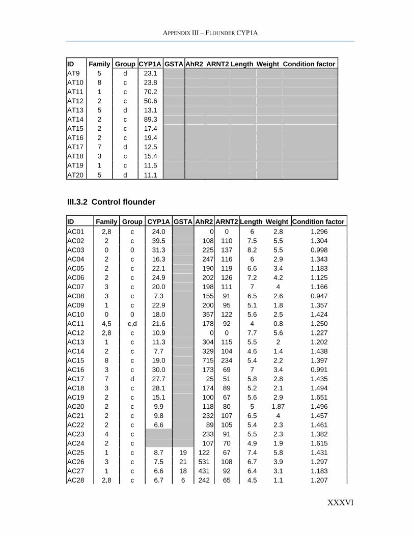
APPENDIX III – FLOUNDER CYP1A
ID Family Group CYP1A GSTA AhR2 ARNT2 Length Weight Condition factorAT9 5 d 23.1 AT10 8 c 23.8 AT11 1 c 70.2 AT12 2 c 50.6 AT13 5 d 13.1 AT14 2 c 89.3 AT15 2 c 17.4 AT16 2 c 19.4 AT17 7 d 12.5 AT18 3 c 15.4 AT19 1 c 11.5 AT20 5 d 11.1
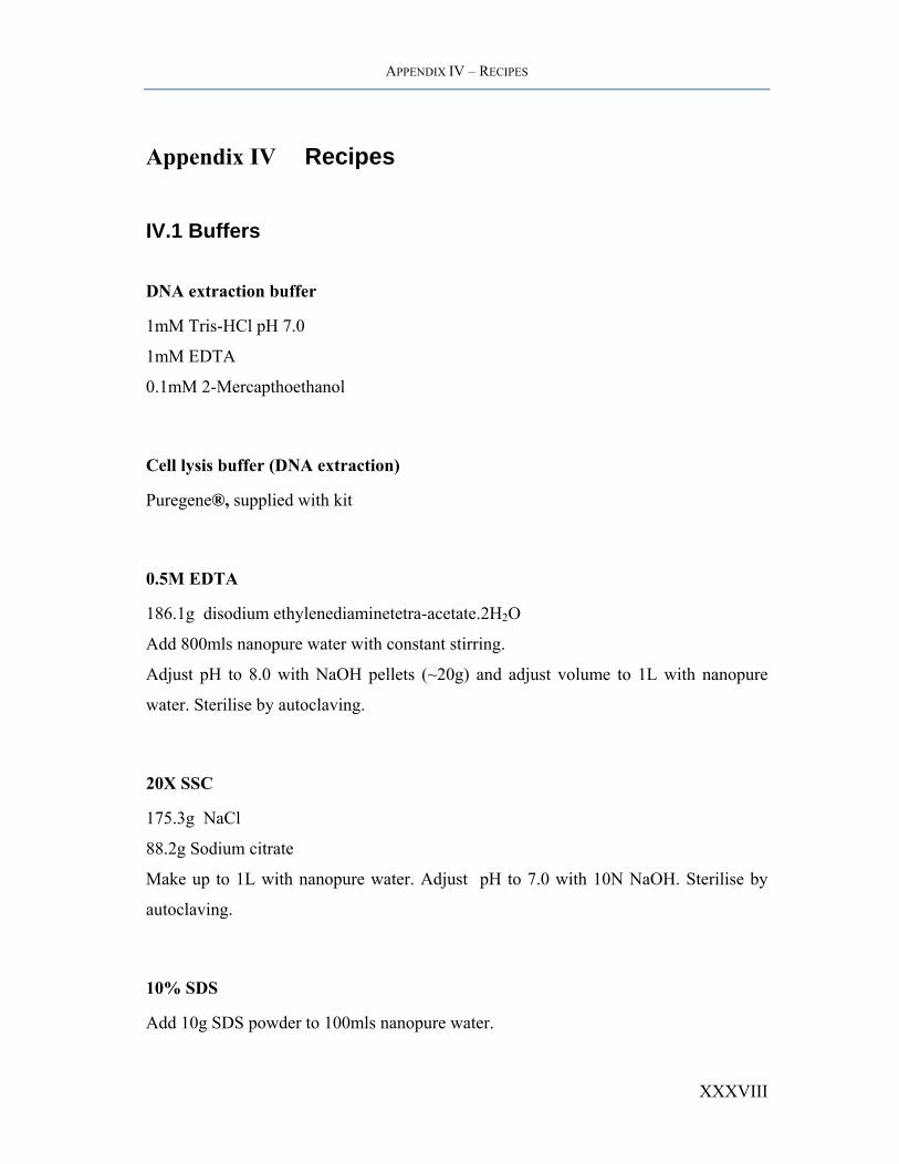
III.3.2 Control flounder
ID Family Group CYP1A GSTA AhR2 ARNT2 Length Weight Condition factorAC01 2,8 c 24.0 0 0 6 2.8 1.296 AC02 2 c 39.5 108 110 7.5 5.5 1.304 AC03 0 0 31.3 225 137 8.2 5.5 0.998 AC04 2 c 16.3 247 116 6 2.9 1.343 AC05 2 c 22.1 190 119 6.6 3.4 1.183 AC06 2 c 24.9 202 126 7.2 4.2 1.125 AC07 3 c 20.0 198 111 7 4 1.166 AC08 3 c 7.3 155 91 6.5 2.6 0.947 AC09 1 c 22.9 200 95 5.1 1.8 1.357 AC10 0 0 18.0 357 122 5.6 2.5 1.424 AC11 4,5 c,d 21.6 178 92 4 0.8 1.250 AC12 2,8 c 10.9 0 0 7.7 5.6 1.227 AC13 1 c 11.3 304 115 5.5 2 1.202 AC14 2 c 7.7 329 104 4.6 1.4 1.438 AC15 8 c 19.0 715 234 5.4 2.2 1.397 AC16 3 c 30.0 173 69 7 3.4 0.991 AC17 7 d 27.7 25 51 5.8 2.8 1.435 AC18 3 c 28.1 174 89 5.2 2.1 1.494 AC19 2 c 15.1 100 67 5.6 2.9 1.651 AC20 2 c 9.9 118 80 5 1.87 1.496 AC21 2 c 9.8 232 107 6.5 4 1.457 AC22 2 c 6.6 89 105 5.4 2.3 1.461 AC23 4 c 233 91 5.5 2.3 1.382 AC24 2 c 107 70 4.9 1.9 1.615 AC25 1 c 8.7 19 122 67 7.4 5.8 1.431 AC26 3 c 7.5 21 531 108 6.7 3.9 1.297 AC27 1 c 6.6 18 431 92 6.4 3.1 1.183 AC28 2,8 c 6.7 6 242 65 4.5 1.1 1.207
XXXVI

APPENDIX III – FLOUNDER CYP1A
ID Family Group CYP1A GSTA AhR2 ARNT2 Length Weight Condition factorAC29 0 0 2.0 6 291 94 4.7 1.8 1.734 AC30 0 0 3.0 14 254 96 7 4 1.166 AC31 2,8 c 14.0 34 391 125 6 3.6 1.667 AC32 0 0 9.0 14 425 127 4.3 1 1.258 AC33 2,8 c 4.9 4 0 2 4 0.6 0.938 AC34 5 d 3.2 14 193 79 8.6 7.2 1.132 AC35 2 c 11.2 22 162 65 7.2 4 1.072 AC36 2 c 10.9 40 294 131 6 2.9 1.343 AC37 0 0 4.5 9 216 116 5 1.4 1.120 AC38 1 c 8.8 30 190 97 5 3.3 2.640 AC39 2 c 7.6 40 151 63 6.4 3.3 1.259 AC40 2 c 5.2 26 209 84 6.5 4.8 1.748 AC41 2 c 8.0 48 251 79 7.4 5.3 1.308 AC42 3,8 c 4.9 35 129 70 8.1 6.3 1.185 AC43 3 c 5.2 13 80 100 5 1.4 1.120 AC44 2 c 2.2 12 172 112 4.9 1.5 1.275 AC45 5 d 3.3 17 0 0 4 0.7 1.094 AC46 2 c 0.5 18 184 95 7.1 4.4 1.229 AC47 2 c 4.4 36 314 151 5.7 2.8 1.512 AC48 1 c 3.5 13 256 71 7.1 4.5 1.257 AC49 2 c 4.2 28 92 48 5.2 3 2.134 AC50 1 c 4.5 13 113 85 4.8 1.7 1.537 AC51 3,8 c 9.4 40 261 119 6.9 3.8 1.157 AC52 0 0 9.2 23 187 117 5.4 2.7 1.715 AC53 0 0 8.3 0 292 155 6 2.8 1.296 AC54 1,2 c 5.9 16 118 71 8.2 6.1 1.106 AC55 2 c 8.3 56 190 59 7.2 4.6 1.232 AC56 0 0 12.7 63 416 88 8.3 7.4 1.294 AC57 0 0 23.6 55 131 39 7.2 4.7 1.259 AC58 3 c 15.4 58 76 24 5.8 2.6 1.333 AC59 0 0 9.7 68 372 126 7 4.1 1.195 AC60 0 0 12.3 165 142 72 6.8 3.9 1.240 AC61 2 c 9.4 38 279 102 6 2.9 1.343 AC62 0 0 9.0 7 185 99 5.7 2.2 1.188 AC63 0 0 5.5 18 203 119 6.6 3.3 1.148 AC64 4,5 c,d 13.2 28 404 116 7.5 5.5 1.304 AC65 7 d 11.4 72 6.6 4.1 1.426 AC66 0 0 16.9 91 6.8 4.1 1.304 AC67 1,2 c 17.5 55 6.2 3 1.259 AC68 0 0 10.1 92 7.4 4.7 1.160 AC69 3,7 c,d 5.2 158 5.9 2.5 1.217 AC70 0 0 7.9 0 4.5 1.2 1.317 AC71 1,2 c 20.8 135 6.8 4.1 1.304 AC72 2 c 20.6 145 6.6 3.6 1.252
XXXVII
APPENDIX IV – RECIPES
Appendix IV Recipes
IV.1 Buffers
DNA extraction buffer
1mM Tris-HCl pH 7.0
1mM EDTA
0.1mM 2-Mercapthoethanol
Cell lysis buffer (DNA extraction)
Puregene®, supplied with kit
0.5M EDTA
186.1g disodium ethylenediaminetetra-acetate.2H2O
Add 800mls nanopure water with constant stirring.
Adjust pH to 8.0 with NaOH pellets (~20g) and adjust volume to 1L with nanopure
water. Sterilise by autoclaving.
20X SSC
175.3g NaCl
88.2g Sodium citrate
Make up to 1L with nanopure water. Adjust pH to 7.0 with 10N NaOH. Sterilise by
autoclaving.
10% SDS
Add 10g SDS powder to 100mls nanopure water.
XXXVIII
APPENDIX IV – RECIPES
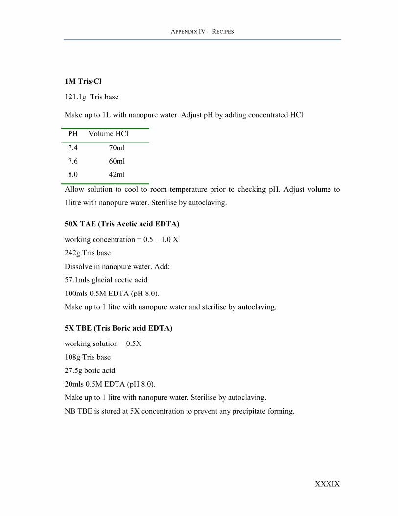
1M Tris·Cl
121.1g Tris base
Make up to 1L with nanopure water. Adjust pH by adding concentrated HCl:
PH Volume HCl
7.4 70ml
7.6 60ml
8.0 42ml
Allow solution to cool to room temperature prior to checking pH. Adjust volume to
1litre with nanopure water. Sterilise by autoclaving.
50X TAE (Tris Acetic acid EDTA)
working concentration = 0.5 – 1.0 X
242g Tris base
Dissolve in nanopure water. Add:
57.1mls glacial acetic acid
100mls 0.5M EDTA (pH 8.0).
Make up to 1 litre with nanopure water and sterilise by autoclaving.
5X TBE (Tris Boric acid EDTA)
working solution = 0.5X
108g Tris base
27.5g boric acid
20mls 0.5M EDTA (pH 8.0).
Make up to 1 litre with nanopure water. Sterilise by autoclaving.
NB TBE is stored at 5X concentration to prevent any precipitate forming.
XXXIX
APPENDIX IV – RECIPES
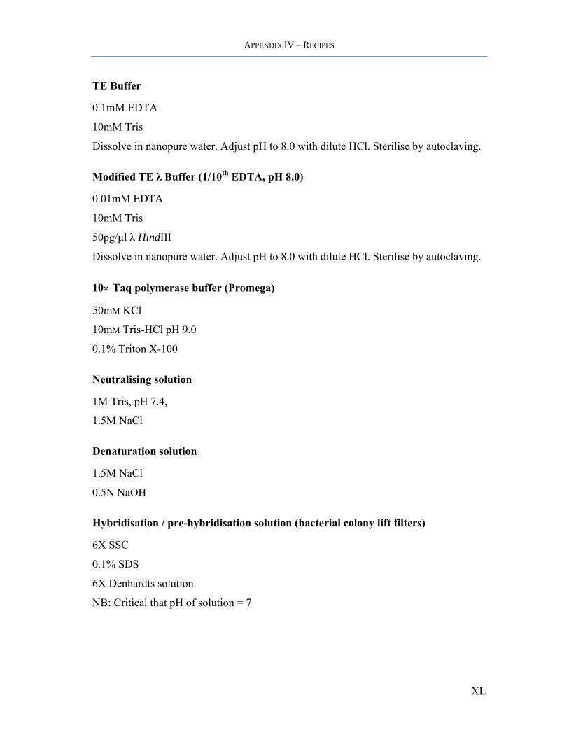
TE Buffer
0.1mM EDTA
10mM Tris
Dissolve in nanopure water. Adjust pH to 8.0 with dilute HCl. Sterilise by autoclaving.
Modified TE λ Buffer (1/10th EDTA, pH 8.0)
0.01mM EDTA
10mM Tris
50pg/µl λ HindIII
Dissolve in nanopure water. Adjust pH to 8.0 with dilute HCl. Sterilise by autoclaving.
10× Taq polymerase buffer (Promega)
50mM KCl
10mM Tris-HCl pH 9.0
0.1% Triton X-100
Neutralising solution
1M Tris, pH 7.4,
1.5M NaCl
Denaturation solution
1.5M NaCl
0.5N NaOH
Hybridisation / pre-hybridisation solution (bacterial colony lift filters)
6X SSC
0.1% SDS
6X Denhardts solution.
NB: Critical that pH of solution = 7
XL

APPENDIX IV – RECIPES
Ethidium Bromide (10mg/ml stock)
1g of ethidium bromide
Make up to 100mls with nanopure water by stirring for several hours. Store at room
temperature in light proof container.
ABI 377 Sequencing Gel Loading Buffer
98% deionized formamide,
10mM EDTA (pH 8.0)
0.025% xylene cyanol FF
0.025% bromophenol blue
10% APS (Ammonium Persulphate)
1g APS
Make up to 10mls with nanopure water.
Solution can be stored for a 2-3 weeks at 4oC.
Proteinase K
Dissolve proteinase K in deionised water to a concentration of 20mg/ml. Store at –
200C.
RNAase A (DNAase free)
Dissolve pancreatic RNAase A at a concentration of 10mg/ml in 0.01M sodium acetate
(pH 5.2). Heat to 1000C for 15 minutes. Allow to cool, slowly, to room temperature.
Adjust the pH by adding 0.1 volumes of 1M Tris·Cl (pH 7.4). Store at –200C.
XLI
APPENDIX IV – RECIPES
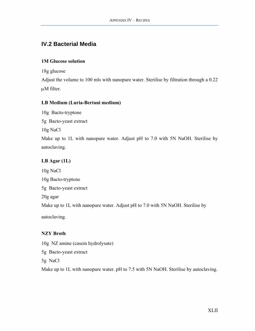
IV.2 Bacterial Media
1M Glucose solution
18g glucose
Adjust the volume to 100 mls with nanopure water. Sterilise by filtration through a 0.22
µM filter.
LB Medium (Luria-Bertani medium)
10g Bacto-tryptone
5g Bacto-yeast extract
10g NaCl
Make up to 1L with nanopure water. Adjust pH to 7.0 with 5N NaOH. Sterilise by
autoclaving.
LB Agar (1L)
10g NaCl
10g Bacto-tryptone
5g Bacto-yeast extract
20g agar
Make up to 1L with nanopure water. Adjust pH to 7.0 with 5N NaOH. Sterilise by
autoclaving.
NZY Broth
10g NZ amine (casein hydrolysate)
5g Bacto-yeast extract
5g NaCl
Make up to 1L with nanopure water. pH to 7.5 with 5N NaOH. Sterilise by autoclaving.
XLII

APPENDIX IV – RECIPES
NZY+ Broth
To a 100ml aliquot of NZY Broth (see above) add the following supplements
immediately before use:
1.25mls 1M MgCl2 filter sterilized
1.25mls 1M MgSO4 f/s
1ml 2M filter sterile glucose
X-gal (5-Bromo-4-chloro-3-indolyl-β-D-galactoside)
Dissolve X-gal in dimethylformamide to make a 20mg/ml solution (use a glass or
polypropylene tube). Wrap in aluminium foil or store in light-tight bottle at –200C.
IPTG (Isopropylthio-β-D-galactoside)
Dissolve 2g of IPTG in 8 mls distilled water. Adjust volume to 10mls with distilled
water and sterilise by filtration through a 0.22-micron filter. Store at –200C.
Ampicillin
Dissolve in deionised water to a concentration of 100mg/ml. Sterilise by filtration
through a 0.22 micron filter. Store at –200C.
Tetracycline
Dissolve in ethanol to a concentration of 5mg/ml. Store at –200C in a light-tight
container.
XLIII

APPENDIX IV – RECIPES
IV.3 Formulae:
Primer Tm calculation:
69.3 + 0.41 x %GC content - (650 / length) = melting temperature
Vector : insert ratio
ng vector x Kb size of insert x Molar ration of insert
Kb size of vector vector
(Xg / µl DNA / [plasmid length in bp × 660]) × 6.022×1023 = y moles / µl
Equation 1: Calculation of plasmid construct copy number
XLIV
APPENDIX V – REAL-TIME PCR
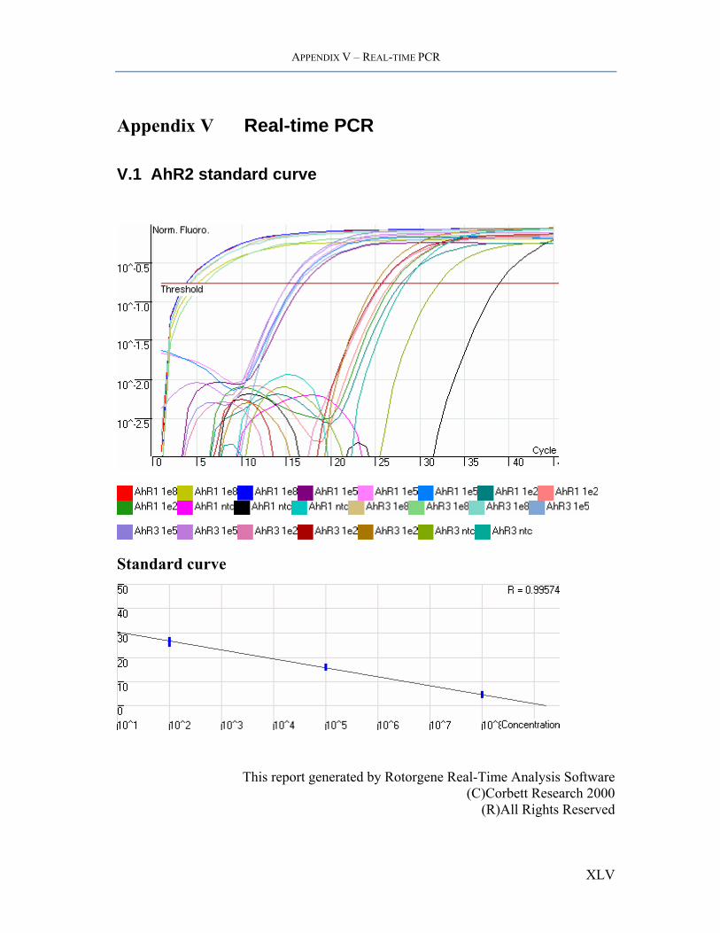
Appendix V Real-time PCR
V.1 AhR2 standard curve
Standard curve
This report generated by Rotorgene Real-Time Analysis Software (C)Corbett Research 2000
(R)All Rights Reserved
XLV
APPENDIX V – REAL-TIME PCR
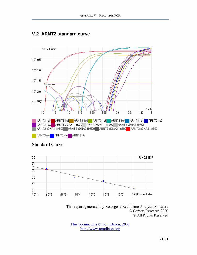
V.2 ARNT2 standard curve
Standard Curve
This report generated by Rotorgene Real-Time Analysis Software
© Corbett Research 2000 ® All Rights Reserved
This document is © Tom Dixon, 2003
http://www.tomdixon.org
XLVI