Embed Size (px)
DESCRIPTION
Appliance Energy Policy Tools 2012
Citation preview

ORIGINAL ARTICLE
Bottom–Up Energy Analysis System (BUENAS)—an internationalappliance efficiency policy tool
Michael A. McNeil & Virginie E. Letschert &Stephane de la Rue du Can & Jing Ke
Received: 30 July 2012 /Accepted: 4 December 2012 /Published online: 9 January 2013# Springer Science+Business Media Dordrecht 2013
Abstract The Bottom–Up Energy Analysis System(BUENAS) calculates potential energy and green-house gas emission impacts of efficiency policies forlighting, heating, ventilation, and air conditioning,appliances, and industrial equipment through 2030.The model includes 16 end use categories and covers11 individual countries plus the European Union.BUENAS is a bottom–up stock accounting model thatpredicts energy consumption for each type of equip-ment in each country according to engineering-basedestimates of annual unit energy consumption, scaledby projections of equipment stock. Energy demand ineach scenario is determined by equipment stock, us-age, intensity, and efficiency. When available, BUE-NAS uses sales forecasts taken from country studies toproject equipment stock. Otherwise, BUENAS uses aneconometric model of household appliance uptakedeveloped by the authors. Once the business as usualscenario is established, a high-efficiency policy
scenario is constructed that includes an improvementin the efficiency of equipment installed in 2015 orlater. Policy case efficiency targets represent current“best practice” and include standards already estab-lished in a major economy or well-defined levelsknown to enjoy a significant market share in a majoreconomy. BUENAS calculates energy savings accord-ing to the difference in energy demand in the twoscenarios. Greenhouse gas emission mitigation is thencalculated using a forecast of electricity carbon factor.We find that mitigation of 1075 mt annual CO2 emis-sions is possible by 2030 from adopting current bestpractices of appliance efficiency policies. This repre-sents a 17 % reduction in emissions in the business asusual case in that year.
Keywords Appliances . Energy demand forecast .
Standards and labeling . Policy best practices .
Appliance diffusion . Developing countries
Introduction
A consensus has emerged among the world’s scientistsand many corporate and political leaders regarding theneed to address the threat of climate change throughemissions mitigation and adaptation. A further con-sensus has emerged that a central component of thesestrategies must be focused around energy, which is theprimary generator of greenhouse gas emissions. Twoimportant questions result from this consensus: “what
Energy Efficiency (2013) 6:191–217DOI 10.1007/s12053-012-9182-6
M. A. McNeil (*) :V. E. Letschert : S. de la Rue du Can :J. KeLawrence Berkeley National Laboratory,1 Cyclotron Rd,Berkeley, CA, USAe-mail: [email protected]
V. E. Letscherte-mail: [email protected]
S. de la Rue du Cane-mail: [email protected]
J. Kee-mail: [email protected]

kinds of policies encourage the appropriate transfor-mation to energy efficiency” and “how much impactcan these policies have”?
Appliance1 efficiency alone will not solve the cli-mate change problem, but it yields itself to markettransformation policies whose success is well estab-lished. For example, appliance standards already writ-ten into law in the USA are expected to reduceresidential sector consumption and carbon dioxideemissions by 8–9 % by 2020 (Meyers et al. 2003).Another study indicates that policies in all OECDcountries will likely reduce residential electricity con-sumption in those countries by 12.5 % in 2020, com-pared to if no policies had been implemented to date(IEA 2003). Studies of impacts of programs alreadyimplemented in developing countries are rare, butthere are a few encouraging examples. Mexico, forexample, implemented its first Minimum EfficiencyPerformance Standards (MEPS) on four major prod-ucts in 1995. By 2005, only 10 years later, standardson these products alone were estimated to have re-duced annual national electricity consumption by 9 %(Sanchez et al. 2007). Finally, China has implementedMEPS and expanded the coverage of its voluntaryenergy efficiency label to over 40 products since2005. In an impact assessment of the program, 11products were included and shown to save a cumula-tive 1,143 TWh by 2020, or 9 % of the cumulativeconsumption of residential electricity to that year andreduce carbon dioxide emissions by more than 300million tons carbon equivalent (Fridley et al. 2007).
BUENAS is an end use energy demand projectionmodel developed by Lawrence Berkeley NationalLaboratory (LBNL). As the name suggests, BUENASis a tool to model energy demand by various types ofenergy consuming equipment and aggregate theresults to the end use, sector or national level. BUE-NAS is designed as a policy analysis tool which cre-ates scenarios differentiated by the level of actionstaken—generally toward higher energy efficiency.Impacts of policy actions towards market transforma-tion are calculated by comparing energy demand in the“business as usual” case to a specific policy case.
BUENAS shares elements with a variety of models,2
including models of energy savings supporting theUSDOE’s appliance standards program. The charac-teristics that distinguish BUENAS are that it coversmultiple countries, models energy demand at the tech-nology level, and projects efficiency improvementbased on specific targets judged to be achievable.
At the time the development of the BUENAS be-gan, there were few examples of attempts to evaluatethe potential impacts of appliance efficiency programsat a global level, although at least one study hadconsidered the program-wide potential in the USA(Rosenquist et al. 2006)3. Since that time, a few seri-ous attempts have been made, but these have generallyfocused on sector energy demand reductions (IEA2010) or adoption of technology measures (McKinsey& Company 2009) without reference to specific effi-ciency policies.
Construction of the BUENAS model represents an-other example to estimate the global potential of appli-ance efficiency policies. The goals of this article are to:
1. Provide background on the objectives and scopeof the BUENAS model
2. Detail the energy forecasting methodology anddata inputs used by BUENAS
3. Describe the high-efficiency scenario and providesavings potential results.
Using the methodology and assumptions describedbelow, we find that mitigation of 984 mt annual CO2
emissions is possible by 2030 from adopting currentbest practices of appliance efficiency policies. Thisrepresents a 17 % reduction in emissions in the busi-ness as usual case in that year.
Modeling objectives
The main objective of the development of BUENAS isto provide a global model with sufficient detail andaccuracy for quantitative assessment of policy meas-ures such as appliance energy efficiency standards andlabeling (EES&L) programs. In most countries whereenergy efficiency policies exist, the initial emphasis ison household appliances and lighting. Often,
1 Throughout this article, “appliance” is a generic term thatincludes energy-consuming equipment installed in residentialand commercial buildings, lighting, and some discrete industrialequipment such as electric motors and distribution transformers.It excludes vehicles and equipment used as a component inindustrial processes.
2 See Mundaca et al. (2010) for a survey of energy-economymodels used to evaluate efficiency policy.3 Since that time, additional studies of appliance efficiencypotential in the USA have been performed (Rohmund et al.2011; Lowenberger et al. 2012).
192 Energy Efficiency (2013) 6:191–217

equipment used in commercial buildings, particularlyheating, ventilation, and air conditioning (HVAC) isalso covered by EES&L programs. In the industrialsector, standards and labeling generally cover electricmotors and distribution transformers, although a fewmore types of industrial equipment are covered bysome programs, and there is a trend toward includingmore of them.
The concept for BUENAS emerged from the exam-ple of the National Energy Savings (NES) componentof analyses supporting US federal rulemakings onMEPS for residential and commercial equipment.4
The NES analysis forecasts equipment sales and aver-age annual unit energy consumption (UEC) of appli-ances either with or without a federal standard. Totalnational energy demand from the two scenarios is thencompared to yield the energy saving potential of thestandard. BUENAS was constructed in an attempt toreplicate this type of analysis at a global scale,employing much less detail for any given appliancetype in a given country.
We emphasize that, while the business as usual(BAU) scenario used in BUENAS represents a bestestimate of future demand, the focus is on energysavings from policy, not on energy demand. In partic-ular, BUENAS is not comprehensive and is not cali-brated to agree with top–down estimates—it onlyincludes appliance types for which savings potentialcan reasonably be assessed, on a country-by-countrybasis. Having said that, BUENAS covers a significantamount of total energy consumption for some sectorsand fuels in some countries.
The bottom–up approach taken by BUENAS notonly improves accuracy in many cases, it is necessi-tated by the nature of the policies commonly appliedto appliances—EES&L. A first step in setting forthany such policy is to define the scope of coveredequipment. For example, while “laundry equipment”may be a reasonable category for top–down modeling,actual EES&L programs act differently on clotheswashers and dryers, and usually discriminate betweenelectric and gas dryers. Furthermore, the energy de-mand and efficiency potential of top versus front-loading clothes washers is significant, so these two
appliances are treated separately if input data allowand later aggregated as a single end use for reporting.
Comparison to other models
BUENAS is somewhat unique in the amount of detailon appliances it provides at the global level. However,it bears some similarity of purpose to other models,especially in the residential sector, and some discus-sions of its relation to other such models are useful.Happily, a recent article systematically compares suchmodels and includes BUENAS as one of its examples(Mundaca et al. 2010). Mundaca et al. divide theworld of “energy-economy” models into four maincategories: (a) simulation, (b) optimization, (c) ac-counting, and (d) hybrid models. BUENAS is catego-rized as a “simulation” model, which provides “adescriptive quantitative illustration, which is basedon exogenously determined scenarios” (p. 307).
Notwithstanding the features of accounting typemodels incorporated in BUENAS, the simulation char-acterization is accurate, since the BUENAS high-efficiency scenario is policy-driven rather than a resultof consumer economic choice. This is in contrast tomodels such as MARKAL, MESSAGE, NEMS, orPRIMES (Seebregts et al. 2001; Messner and Strubeg-ger 1995; USDOE 1995; Capros 2000), which assumethat consumers act according to economic self-interestat least to some extent. On the other hand, BUENASmodels well-defined efficiency targets generally deter-mined by engineering rather than financial considera-tions. While such options are usually shown to be costeffective in the jurisdiction where they are mandated, itis not assumed that consumers will choose them in theabsence of additional policy. In fact, the BUENASbusiness as usual scenario includes market failuresand/or transaction costs that result in consumers nottaking advantage of good investments because of lackof information, “principal agent” problems, or otherbarriers to adoption of efficient technologies. The rea-sons that energy end users may not pursue pure eco-nomic interest by investing in efficient equipment thatprovides a long-term benefit is the subject of consider-able investigation and debate and is beyond the scope ofthis article. It is valuable, however, to clearly positionBUENAS in this context. The working assumption ofthe BUENAS high-efficiency scenario is that well-designed and implemented policies will eliminate trans-action costs and lower barriers and thus transform the
4 See for example USDOE (2011a). All analyses supporting USDepartment of Energy appliance rulemakings can be found athttp://www1.eere.energy.gov/buildings/appliance_standards/.
Energy Efficiency (2013) 6:191–217 193

market. In this way, the reliance on an exogenous policyconstruction is not a simplification in BUENAS, rather adesign element appropriate to its purpose as a tool toevaluate policy instead of market effects.
Geographical and end use scope
BUENAS covers 11 countries individually and includesthe 27 Member States of the European Union modeledas a single region. Countries currently included in BUE-NAS are Australia, Brazil, Canada, European Union,India, Indonesia, Japan, Republic of Korea, Mexico,Russia, South Africa, and the USA. Chinese applianceenergy demand and efficiency potential has also beenmodeled in detail by LBNL (Zhou et al. 2011a). LBNL’sChina appliance model is a component of the China2050 EnergyModel (Zhou et al. 2011b), which includesall energy demand sectors.
Since the model covers most of the world’s largeeconomies, the fraction of global energy consumptionrepresented by modeled countries is large. Accordingto IEA data on total energy demand in 2005(Interna-tional Energy 2006a), the countries covered accountfor 62 % of global final energy demand if China is notincluded. Including China, country energy coverage is77 % of global energy demand. The breakdown ofenergy demand percentage by countries included inBUENAS is shown in Table 1.
BUENAS includes a wide range of energy-consuming products, including most end uses gener-ally covered by EES&L programs around the world.End uses currently covered are:
& Residential sector: air conditioning, cooking +dishwashing, fans, lighting, refrigeration, spaceheating, standby, televisions, water heating, andlaundry
& Commercial building sector: air conditioning,lighting, refrigeration, space heating, and laundry
& Industrial sector: electric motors and distributiontransformers.
An earlier “regional” version of BUENAS (McNeilet al. 2008) estimated each end use listed above forevery region, even in the absence of data. This versionof the model made extensive use of proxy data; that is,the assumption that data for one country applies to theentire region and in some cases to multiple regions. Inthe current version of the model, the strategy priori-tizes accuracy over comprehensiveness and thereforeminimizes the use of proxy data with the consequencethat significant gaps remain in the coverage. In fact,some of the end uses listed above are modeled for onlyone or two countries. A continuing effort will be madegoing forward to address these gaps as reliablecountry-specific data are made available. Table 2 sum-marizes the end use coverage in the current version of
Table 1 Energy consumptionpercentage by countries includedin BUENAS
Source: International EnergyAgency (2006a), 2005 data
Region % Energy Country % Energy
Pacific OECD 8 Australia 1.1
Japan 4.6
Korea 1.9
North America 23 United States 20.5
Canada 2.4
Western + Eastern Europe 17 European Union 15.6
Former Soviet Union 9 Russia 5.7
Latin America 6 Mexico 1.5
Brazil 1.8
Sub-Saharan Africa 3 South Africa 1.1
Middle East + No. Africa 5 – –
Centrally-Planned Asia 16 China 15.0
South Asia—Other Pacific Asia 9 India 4.7
Indonesia 1.6
Total 96 Total without China 62
Total including China 77
194 Energy Efficiency (2013) 6:191–217

the model by country/economy. Country abbreviationsare defined by the International Standards Organiza-tion: Australia (AUS), Brazil (BRA), Canada (CAN),European Union (EU), Indonesia (IDN), India (IND),Japan (JPN), Republic of Korea (KOR), Mexico(MEX), Russia (RUS), United States of America(USA), and South Africa (ZAF).
The main objective of the development of BUE-NAS is to provide a global model with sufficientdetail and accuracy for technical assessment ofpolicy measures such as EES&L programs. Inmost countries where energy efficiency policiesexist, the initial emphasis is on household appli-ances and lighting. Often, equipment used in com-mercial buildings, particularly HVAC, is alsocovered by EES&L programs. In the industrialsector, standards and labeling generally coverselectric motors and distribution transformers, al-though a few more types of industrial equipmentare covered by some programs, and there is atrend toward including more of them. In order tomake a comprehensive estimate of the total poten-tial impacts, development of the model prioritizedcoverage of as many end uses commonly targetedby EES&L programs as possible, for as manycountries as possible. The model generally didnot cover:
& Industrial processes& ‘Miscellaneous’ end uses or end uses not typically
included in EES&L programs.
Data regarding additional end uses is continuallybecoming available, particularly in the commercialand industrial sector, leading to an ongoing opportu-nity (and need) to expand and update BUENAS.
Energy demand forecast
BUENAS projects energy demand in order to calcu-late impacts of current, proposed or possible policies.National energy demand of each end use is con-structed according to the following modification ofthe Kaya identity (Kaya 1989).
Energy ¼ Activity� Intensity
Efficiency
In this equation, Activity refers to the size of thestock, e.g., number of refrigerators or the air condi-tioned area of commercial buildings. Intensity is driv-en by the usage and capacity of each unit, such as thesize of a water heater or the hours of use of a room airconditioner. Finally, Efficiency is the technologicalperformance of the equipment, which can be affectedby government policies.
BUENAS is implemented using the Long-RangeEnergy Alternatives Planning system (LEAP), devel-oped by the Stockholm Environment Institute.5 LEAPis a general-purpose energy accounting model inwhich the model developer inputs all data and assump-tions in a format that is then transparent to other users.
BUENAS projects energy consumption by end usefrom 2005 (base year) to 2030. The strategy of themodel is to first project end use activity, which isdriven by increased ownership of household applian-ces, and economic growth in the commercial andindustrial sectors. The total stock of appliances canbe modeled either according to an econometric diffu-sion equation or according to unit sales projections if
Table 2 BUENAS end-use/economy coverage
Sector End Use Category AUS BRA CAN EU IND IDN JPN KOR MEX RUS USA ZAFResidential Air Conditioning 12.4 17.99 16.93 17.72 99.68 8.393 300.7 19.69 16.04 1.626 41.8 6.603
Fans 0.368 10.04 0.329 3.315 64.34 7.437 1.68 0.784 2.868 1.064 25.38 1.237Laundry 0 0 0 45.96 0 0 0 5.143 1.864 0 99.09 0Lighting 4.72 29.03 10.72 64.34 55.32 32.81 24.97 9.431 15.65 12.62 81.64 6.124Refrigerators & Freezers 6.284 55.32 14.58 84.23 18.28 8.238 34.77 17.55 8.837 22.92 126.5 5.833Space Heating 0 0 15.07 1689 0 0 1323 0 0 0 235.1 0Standby 1.535 7.227 2.403 58.58 22.42 4.497 7.488 2.951 3.297 5.759 43.64 1.119Television 10.48 8.416 5.371 39.74 10.15 2.347 8.101 7.45 4.501 6.179 17.89 1.077Water Heating 15.58 0 41.31 672.3 0 0 128.1 0 140.8 0 322.2 0
Commercial Air Conditioning 9.824 30.95 17.19 148 17.66 14.42 66.3 27.39 19.3 17.37 305.1 2.499Lighting 21.74 34.25 37.03 233.2 17.44 13.34 81.99 39.67 23.47 45.33 500.6 4.897Refrigeration 4.855 7.721 8.485 111.1 3.903 2.953 18.87 8.888 5.291 10.48 104.5 1.102
Industry Distribution Transformers 12.82 0 13.82 0 10.27 0 43.08 19.45 13.13 43.46 368.6 0Motors 60.9 201.7 101 830.8 396 155.5 314.3 158.5 89.92 274.3 826.6 44.99
5 For more information on LEAP, visit http://www.sei-us.org/software/leap.html
Energy Efficiency (2013) 6:191–217 195

such forecasts are available. Electricity consumptionor intensity of the appliance stock is then calculatedaccording to estimates of the baseline intensity of theprevailing technology in the local market. Finally, thetotal final energy consumption of the stock is calcu-lated by modeling the flow of products into the stockand the marginal intensity of purchased units, either asadditions or as replacements of old units according toequipment retirement rates. The high efficiency or “pol-icy” scenario is created by the assumption of increasedunit efficiency relative to the baseline starting in a cer-tain year. For example, if the average baseline UEC ofnew refrigerators is 450 kWh/year, but a MEPS takingeffect in 2012 requires a maximum UEC of 350 kWh/year, the stock energy in the policy scenario will grad-ually become lower than that of the base case scenariodue to increasing penetration of high-efficiency unitsunder the standard. By 2030, the entire stock will gen-erally be impacted by the standard.
The two main outputs of BUENAS are national-levelfinal energy savings and carbon dioxide emissions mit-igation. Final energy (electricity or fuel) savings is
important because final energy demand is the driver ofcapital-intensive generation capacity additions and fuelimports. Final energy demand is also the quantitydirectly paid for by consumers. Carbon dioxideforms the majority of greenhouse gas emissionsand is therefore the most important environmentalimpact of energy consumption. The model de-scribed in this article does not calculate financialimpacts of efficiency policy due to the datarequirements needed to include them. However,financial impacts are planned in future versionsof the model. Primary energy inputs to electricityare also not considered, although carbon emissionsare a rough proxy for them.
The legend of Fig. 1 shows the different componenttypes of the model. These are:
1. Data or assumption—These are direct inputs tothe model. In the case of data from other sources,the reference of the primary data source is listed.In cases where no data are available, assumptionsare sometimes made.
Unit Sales
Baseline Unit Energy
Consumption
CO2
Mitigation
Final Energy Savings
Carbon Factor
Retirement(Survival) Function
Business as UsualEnergy Final
Energy Demand
Efficiency Case Final Energy
Demand
Target Unit Energy
Consumption
Stock
Diffusion
GDP/capitaElectrificationUrbanization
LEGEND
Data orAssumption
Calculation
Data or Calculation
Fig. 1 Flowchart of BUENAS calculation. Note: Stock and Diffusion can be entered directly into the model as data, but this is rare
196 Energy Efficiency (2013) 6:191–217

2. Calculation—These are computations governedby the equations in the previous section.These are either built into LEAP, or areuser-defined.
3. Data or calculation—This can be either a directdata input or a calculation. The main example ofthis is the projection of unit sales. When available,these data are input directly in the model. If nosuch data are available, sales are modeled fromstock as an intermediate result. Stock in turn canbe a direct input or from a model of applianceownership (diffusion).
Residential sector model
BUENAS calculates final energy demand according tounit energy consumption of equipment sold in previ-ous years:
EBAUðyÞ ¼X
age
Sales y� ageð Þ � UECBAU y� ageð Þ � Surv ageð Þ
& EBAU(y) = final energy demand in the business asusual scenario in year y
& Sales(y) = unit sales (shipments) in year y& UEC(y) = unit energy consumption of units sold in
year y& Surv(age) = probability of surviving to age years.
When unit sales (shipments) are not given as directdata inputs then BUENAS derives them fromincreases in stock and replacements:
SalesðyÞ ¼ StockðyÞ � Stock y� 1ð ÞþX
age
Ret ageð Þ � Sales y� ageð Þ
& Stock(y) = number of units in operation in year y& Ret(age) = probability that a unit will retire (and be
replaced) at a certain age.
Survival function and retirement function arerelated by:
Surv ageð Þ ¼ 1�X
age
Ret ageð Þ
Three different methods are used to estimate thetotal stock of a particular residential end use. Foreach region and end use, the highest accuracymethod is chosen for which sufficient data are
available. In order of decreasing accuracy, themethods are:
1. Stock based on historical and projected flowsof products (unit sales)
2. Stock from historical and projected ownershiprates—sales derived from stock increases andreplacement rates
3. Stock from econometric modeling driven bymacroeconomic trends—sales derived fromstock increases and replacement rates.
Stock is rarely given directly as input data. Instead,if sales data are not available, BUENAS uses appli-ance diffusion (ownership) rates:
StockðyÞ ¼ DiffusionðyÞ � HHðyÞ
& Diffusion(y) = number of units (owned and used)per household in year y
& HH(y) = Number of households in year y.
In turn, diffusion rates are generally not given byinput data, but are projected according to a macroeco-nomic model:
Diffusion yð Þ ¼ a1þ g � exp b1 � IðyÞ þ b2 � UðyÞ þ b3 � EðyÞ½ �
& I(y) = household income (GDP per household) inyear (y)
& U(y) = urbanization rate in year (y)& Elec(y) = electrification rate in year (y)& α,γ,β1,β2,β3 = model parameters (described in
McNeil and Letschert 2010).
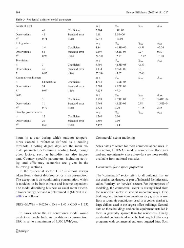
The determination of diffusion coefficients for allmodeled equipment types is shown in Table 3.
In the case of fans, cooling degree days areused as a driving variable of ownership. Air con-ditioner ownership is also highly climate depen-dent. To model this, the diffusion equation for airconditioners is multiplied by a climate maximumparameter ranging from 0 to 1. Climate maximumis given by the following equation, as determinedin (McNeil and Letschert 2010)
ClimateMaximum ¼ 1:0� 0:949� expð�0:00187 � CDDÞ
This equation utilizes the climate parametercooling degree days (CDD), which integrates total
Energy Efficiency (2013) 6:191–217 197
hours in a year during which outdoor tempera-tures exceed a reference defined as a coolingthreshold. Cooling degree days are the main cli-mate parameter determining cooling load, thoughother factors, such as humidity, are also impor-tant. Country specific parameters, including activ-ity, and efficiency scenarios are given in thefollowing sections.
In the residential sector, UEC is almost alwaystaken from a direct data source, or is an assumption.The exception is air conditioning consumption, whichis modeled to be both climate and income dependent.The model describing business as usual room air con-ditioner energy demand is determined in (McNeil et al.2008) as follows:
UECðyÞ kWhð Þ ¼ 0:0276� IðyÞ þ 1:46� CDD� 1; 332
In cases where the air conditioner model wouldpredict extremely high air conditioner consumption,UEC is set to a maximum of 3,500 kWh/year.
Commercial sector modeling
Sales data are scarce for most commercial end uses. Inthis sector, BUENAS models commercial floor areaand end use intensity, since these data are more readilyavailable from national statistics.
Commercial floor space projection
The “commercial” sector refers to all buildings that arenot used as residences, or part of industrial facilities (alsocalled “tertiary” or “service” sector). For the purposes ofmodeling, the commercial sector is distinguished fromthe residential sector in several important ways. First,buildings and end use equipment can vary greatly in size,from a room air conditioner used in a corner market tolarge chillers used in the largest office buildings. Second,data on these buildings and on the equipment installed inthem is generally sparser than for residences. Finally,residential end uses tend to be the first target of efficiencyprograms with commercial end uses targeted later. Such
Table 3 Residential diffusion model parameters
Points of light ln γ βInc βElec βUrbα 40 Coefficient 2.204 −3E−05Observations 42 Standard error 0.18 3.0E−06R2 0.71 t-Stat 12.45 −10.00Refrigerators ln γ βInc βElec βUrbα 1.4 Coefficient 4.84 −1.3E−05 −3.59 −2.24Observations 64 Standard error 0.197 4.82E−06 0.27 0.59
R2 0.92 t-Stat 24.508 −2.77 −13.42 −3.78Televisions ln γ βInc βElec βUrbα 3 Coefficient 3.701 −2.5E−05 −2.39Observations 46 Standard error 0.134 4.96E−06 0.31
R2 0.85 t-Stat 27.584 −5.07 −7.66Room air conditioners ln γ βInc βElec βUrbα ClimateMax Coefficient 4.843 −6.9E−05Observations 24 Standard error 0.503 9.82E−06R2 0.69 t-Stat 9.635 −7.04Fans ln γ βInc βElec βCDDα 3 Coefficient 0.798 9.79E−07 −1.13 3.41E−04Observations 11 Standard error 0.968 4.82E−06 0.98 1.34E−04R2 0.79 t-Stat 0.824 0.20 −1.15 2.55
Standby power devices ln γ βInc βElec βUrbα 12 Coefficient 1.266 0.00
Observations 20 Standard error 0.508 0.00
R2 0.40 t-Stat 2.492 −3.43
198 Energy Efficiency (2013) 6:191–217

programs are an important source of insight into theconsumption and further savings potential of upcomingprograms.
EBAU ¼X
age
Turnover y� ageð Þ � uecBAU y� ageð Þ � Surv ageð Þ
& Turnover(y) = equipment floor space coverageadded or replaced in year y
& uec(y) = energy intensity (kWh/m2) of equipmentinstalled in year y (lower case used to distin-guished from unit energy consumption, UEC).
Much of the focus of commercial building modelingis on the projection of commercial floor space. Whilecurrent floor space estimates are available for somecountries, in general projections are not. The strategyfor determining floor space is to separately model thepercentage of employment in the tertiary sector of theeconomy and the floor space per employee engaged inthis sector. Service sector share (SSS) is multiplied bythe total number of employees which is determined by:
& Economically active population PEA(y) from theInternational Labor Organization projected to2020 and extrapolated thereafter (ILO 2007)
& Unemployment rate RU(y) from the InternationalLabor Organization (ILO 2007) till 2005, and pro-jected to 2005 regional average by 2020.
SSS is modeled as a function of GDP per capita interms of purchasing power parity (PPP). SSS data areavailable from the World Bank for a wide range ofcountries and for different years. The relationship be-tween SSS and GDP per capita is modeled in the formof a log-linear equation of the form
SSSðyÞ ¼ a� ln IðyÞ½ � þ b
The parameters a and b are determined to be 0.122and −0.596, respectively. More detail about the dataused to determine these parameters can be found in(McNeil et al. 2008).
Using these components, the number of servicesector employees NSSE is given by
NSSEðyÞ ¼ PEAðyÞ � 1� RU ðyÞ½ � � SSSðyÞFloor space per employee, denoted f(y) is, like SSS,
assumed to be a function of per capita income only.The relationship assumes a logistic functional form:
f ðyÞ ¼ a
1þ g � exp b0 0 � iðyÞ� �
In this equation, the maximum value α is set to 70 m2
per employee, which was larger than any of the observeddata. The variable I denotes GDP per capita, and β″ andγ were determined to be −9.9×10⁻⁵ and 6.04, respec-tively. More detail about the data used to determine theseparameters can be found in (McNeil et al. 2008).
Turnover is driven by increases in floor space, andreplacement of existing equipment occupying floorspace.
TurnoverðyÞ ¼ FðyÞ � F y� 1ð Þ þPage
RetðageÞ�Turnover y� ageð Þ
& F(y) = total commercial floor space in year y.
Commercial end use intensity
Generally, it is difficult or nearly impossible to modelcommercial end use intensity according to stock flows ofspecific equipment types due to data limitations. There-fore, end use intensity estimation takes an aggregateapproach. End-use intensity is composed of penetration,efficiency, and usage. Penetration takes into account theeffect of economic development on increased density ofequipment expressed in Watts per square meter and isassumed to be a function of GDP per capita only. Rela-tive efficiency is estimated from specific technologiesand usage is given by hours per year. Savings betweenthe high-efficiency and the business as usual case arisefrom percentage efficiency improvements.
Lighting efficiency is estimated as the fraction inthe stock of lighting types: T12, T8, and T5 fluores-cent tubes, incandescent lamps, compact fluorescentlamps, halogen lamps, and other lamps. In addition,relative efficiency of fluorescent lamp ballasts contrib-utes to overall lighting efficiency. Assumptions forlighting energy intensity and the subsequent calcula-tion of penetration are provided in McNeil et al.(2008). The result is a model of penetration accordingto a logistic function
p W m2�� � ¼ a
1þ g � eb�IðyÞ
The variable I(y) denotes GDP per capita, and α, β,and γ are found to be 16.0, −7.78×10⁻⁵, and 3.55,respectively.
Space cooling energy intensity is of course a strongfunction of not only climate but also economic devel-opment. Its dependence on cooling degree days (CCD)
Energy Efficiency (2013) 6:191–217 199

is assumed to be linear. The dependence on GDP percapita, which we call “availability,” takes a logisticform:
Int kW m2�� � ¼ a
1þ g � eb�IðyÞ � aþ b� CCDð Þ
In order to separate the effect, the climate depen-dence is determined from US data, where availabilityis assumed to be maximized. Once modeled in thisway, the climate dependence can be divided out offinal energy intensity data to yield availability as afunction of GDP per capita. The parameters for spacecooling intensity determined in this way are:
a ¼ 1:8; b ¼ 0:00011; g ¼ 8:83; a ¼ 9:7193; b ¼ 0:0123
Space cooling efficiency is determined according toestimates of market shares of room air conditioners,central air conditioners and chillers, prevailing base-line technologies and feasible efficiency targets (seeMcNeil et al. 2008)
Due to a scarcity of data for commercial refrigera-tion, space cooling penetration is assumed to have thesame shape as lighting, that is, the availability of spacecooling increases as a function of per capita GDP inthe same proportion as for lighting, but with a differentcoefficient of proportionality A.
Int kWh m2�� � ¼ A
1þ gebIðyÞ
The penetration curve is then calibrated to datafrom the USA, which has a refrigeration intensity of9.94 kW/m2. The resulting value of A is 10.61 kW/m2.In the high efficiency scenario, an improvement of34 % is assumed to be possible (Rosenquist et al.2006) in all countries.
Industrial model
The main industrial type of equipment modeled byBUENAS is electric motors, which are thought toaccount for around half of the industrial electricityconsumption in most countries. Motors modeled rangefrom 1 to over 250 HP and are used in both manufac-turing and lighter industry or commercial applications.They generally exclude smaller motors used as com-ponents in other equipment. In addition to motors,distribution transformers are categorized as industrialequipment although these are sometimes categorized
as commercial sector equipment depending on theirapplication.
Industrial motors model
When sales data and unit energy consumption are notavailable for industrial motors, they are modeled as afunction of industrial value added GDP:
EðyÞBAU ¼ GDPðyÞIND � "� p
& GDP(y)IND = GDP value added of industrial sectorin year (y)
& ε = electricity intensity per unit of industrial GDP& p = percentage of electricity from electric motors
Electricity demand and savings potential for elec-tric motors is treated in the same way for all regionsexcept for the European Union, for which a motorstock projection is provided in the Ecodesign prepara-tory study (de Ameida et al. 2008). The model forindustrial motor activity used in BUENAS is some-what simplistic. For all countries outside of the EU,total electricity consumption of motors as a fraction ofindustrial electricity is used as the activity variable,according to the following formula:
ElecðyÞ ¼ GDPVAINDðyÞ � "� p
In this equation, GDPVAIND is the value added toGDPfrom the industrial sector. The variable ε is the electricityintensity of the industrial sector, that is, the amount ofelectricity consumed for each dollar of industrial valueadded. This variable is taken from historical energy con-sumption data (from IEA) and divided by GDPVAIND
from the World Bank in the base year. Multiplying εand GDPVAIND for the base year simply gives backreported industrial electricity consumption in that yearand, since ε is assumed constant, industrial electricityconsumption in the projection simply grows at the samerate as GDPVAIND. The fraction p is the percentage ofindustrial electricity passing through motors. Multiplyingthe three variables together then gives motor electricityconsumption in each year through 2030.
Distribution transformers model
For some countries, per-unit sales of each category ofdistribution transformers is forecast and unit energylosses can be used to directly calculate energy losses
200 Energy Efficiency (2013) 6:191–217

and savings due to efficiency. Most often, however,these data are not available. In that case, BUENASmodels distribution transformer simplistically accord-ing to exogenous national electricity demand forecastsprovided by (EIA 2008). Since virtually all of theelectricity used in all sectors eventually passes throughat least one distribution transformer, losses throughtransformers in each year y are given by the followingequation:
LossesðyÞ ¼ 1� effð Þ � DemandðyÞIn this equation, eff is the efficiency of transform-
ers, including both load and no-load losses averagedover the load profile. Demand(y) is the total nationalelectricity demand and Losses(y) is the electricity lostthrough all distribution transformers. Finally, in caseswhere neither unit level data nor electricity forecastsare available, distribution transformers are omitted.
Efficiency scenarios
The BAU forecast scenario modeled by BUENAScombines activity forecasts with intensity as modeledor determined by data inputs or assumptions. The baseyear for the BAU forecast is 2010. BUENAS general-ly assumes that baseline efficiency is constant or “fro-zen” at 2010 values over the forecast period and thatthere are no major technology or product class shifts inthat time. Some exceptions include:
& Equipment forecasts from the USA, which aretaken from other studies and often include projec-tions of baseline efficiency improvement andproduct class shifts
& Phase out of incandescent lamps, which isexpected to gradually occur over the forecast peri-od even in the BAU case
& Evolution of product classes towards split room airconditioners and frost-free refrigerators in India.
Of course, the BAU forecast is itself not expectedto remain constant over time. For instance, ongoingregulations are continually improving appliance effi-ciency in major economies. Although these areknown, for practical reasons, we chose not to contin-ually update the baseline, instead choosing to create aseparate scenario quantifying the impact of recentregulations (Kalavase et al. 2012).
A second scenario modeled by BUENAS considersthe potential impacts of regulations in the near tomedium term. This scenario includes efficiencyimprovements judged to be ambitious but achievablefor all countries6. There are many possible ways ofdefining global potential, including cost effectiveness,removal of a certain fraction of low-efficiency modelsfrom the market, or adoption of best available tech-nology. Due to data limitations, the most practicalapproach has been to rely on an evaluation of bestpractices. The best practice (BP) scenario assumes thatall countries achieve stringent efficiency targets by2015, where ‘stringent’ is interpreted in the followingway:
1. Where efficiency levels are comparable globally:the most stringent standard issued by April 1,2011 anywhere in the world.
2. Where they are comparable only within regions ortesting regime: the most stringent comparablestandard issued by April 1, 2011.
3. In the case where an obvious best comparablestandard was not available, an efficiency levelwas set that was deemed to be aggressive orachievable, such as the most efficient products inthe current rating system.
In addition, the best practice scenario assumes thatstandards are further improved in the year 2020, by anamount estimated on a product-by-product basis. Thisscenario either assumes that the same level of im-provement made in 2015 is repeatable in 2020 orassumes that a specific target, such as current “bestavailable technology,” is reached by 2020. Some ofthe policies available to achieve high efficiency targetsinclude:
& Minimum Efficiency Performance Standards(MEPS)—Equipment is required to perform atthe level of efficiency determined by the standard.Products failing to demonstrate compliance arebanned from the market.
& Comparative labels—Comparative labels provideinformation to the consumer about efficiency levelof all products, and boost the efficiency of the
6 In this scenario, “achievable” means that it would be feasibleto implement a policy by that time. The definition does not takeinto account the lead times between policy announcement andimplementation, which can be several years in some countries.
Energy Efficiency (2013) 6:191–217 201

market by generating consumer preference to-wards more highly-rated models.
& Endorsement labels—Endorsement labels repre-sent a “seal of approval” issued by the governmentor an independent entity. Only those models ofvery high efficiency are awarded the label. Theselabels improve the average market efficiency byraising the market share of the highest performingequipment.
These program types are discussed in detail else-where (see Wiel and McMahon 2005), and we do notdiscuss them further here. It is worth noting, however,that, due to the complexity of the number of regions,sectors and end uses considered, we make the simpli-fying assumption that the entire market reaches theefficiency target in the implementation year—an as-sumption that corresponds to the implementation of aMEPS program, although other programs couldachieve the same result if they were able to move themarket average to the same level.
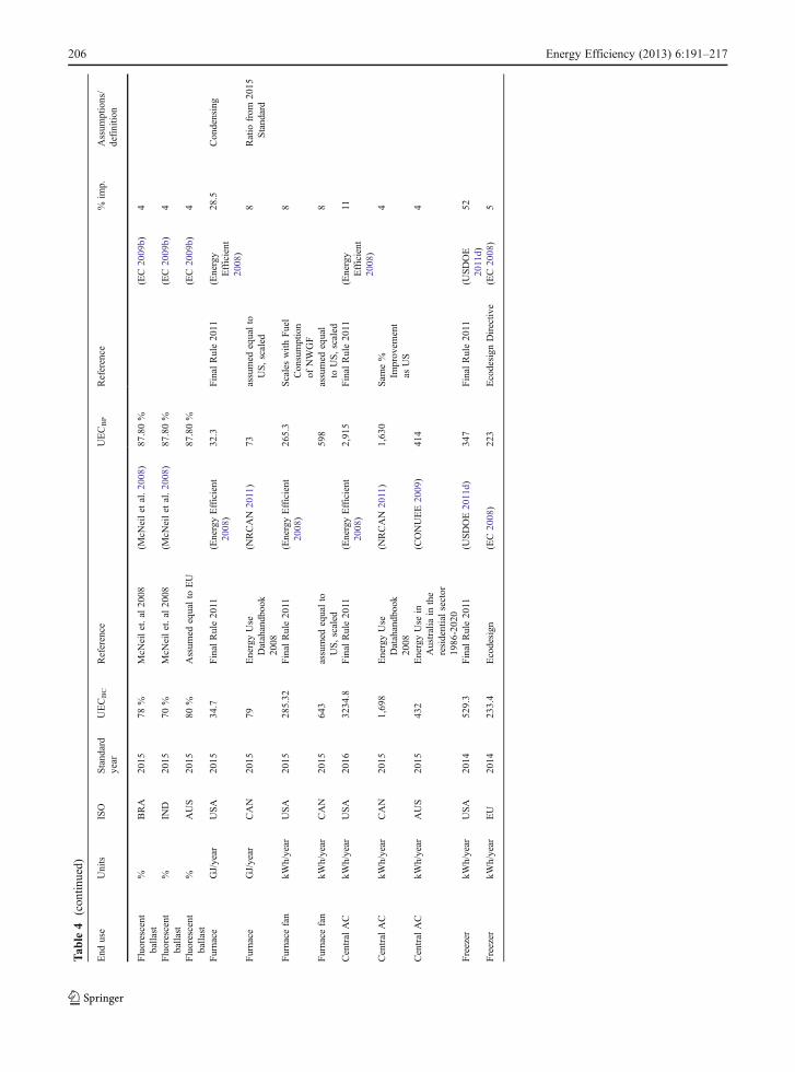
Table 4 summarizes the references and assumptionsused in modeling the best practice scenario. The fol-lowing variables are shown:
End use Appliance type covered by theregulation
Units Metric used to define efficiencylevel (energy consumption or directefficiency metric)
ISO International Standards Organizationthree-letter country code
Standard year Year that regulation takes effectUECBC Unit Energy consumption in the
business as usual case7
Reference Source of unit energy consumptiondata
UECBP Unit energy consumption in the bestpractice scenario
% Imp Percentage improvement betweenbusiness as usual case and recentachievements scenario
Assumptions/definition
Definitions provided by regulatorydocuments or assumptions maderegarding best practice indeveloping the scenario
The most detailed and data-intensive analyses ofthe potential impacts of standards and labeling pro-grams take cost effectiveness into account in an inte-gral way, often defining the optimum policy in termsof “economic potential,” that is, the market transfor-mation that maximizes net economic benefits to con-sumers.8 These benefits can be quantified by a varietyof different metrics, including least life cycle cost, costof conserved energy, or benefit to cost ratios. Due todata constraints, this type of analysis was not possiblehere. Inclusion of costs that will allow this type ofanalysis is anticipated in future versions of the model.Instead, the BP scenario emphasizes the setting ofrealistic, achievable goals. While cost effectiveness isnot considered explicitly, the degree to which thetransformation of the market to a new technology isachievable is implicitly dependent on the cost effec-tiveness of the technology.
Two specific corrections are not taken into accountin these scenarios. First, we do not assume improve-ment in efficiency in the absence of a program. Whilein some cases the 2010 baseline is higher than thecurrent level (due to already scheduled standards),between 2010 and 2020, we assume that the baselineefficiency is constant. Historically, there is generally(but not always) a gradual trend towards higher effi-ciency from market forces alone, but this increasetends to be small in comparison to the increase pro-pelled by EES&L programs. On the other hand, thetargets that we specify in the high efficiency scenarioare already known to exist and to be cost effective insome markets. More often than not, markets overshootthe targets due to learning by manufactures in the timebetween promulgation and implementation of stand-ards.9 These two effects are very difficult to predict,especially for a wide range of regions and end uses.Unpredictably high efficiency in the base case andpolicy case also tend to compensate for one another.In fact, it can be argued that they are both effects of thesame learning process in the manufacturing industryand should therefore, at least on average, tend tocancel each other out.
7 While efficiency is generally assumed to be constant in thebusiness as usual case, unit energy consumption can changeover time according to usage trends.
8 Examples of these are analyses of potentials for the USA(Rosenquist et al. 2006) and IEA countries (IEA 2003).9 There are other reasons as well. For example, evidence sug-gests that manufacturers in Mexico outperformed MEPS in thatcountry in order to produce products competitive in the widerNorth American Market—see Sanchez et al. (2007).
202 Energy Efficiency (2013) 6:191–217

Tab
le4
Referencesanddefinitio
nsof
bestpracticescenario
End
use
Units
ISO
Standard
year
UECBC
Reference
UECBP
Reference
%im
p.Assum
ptions/
definitio
n
Refrigerators
kWh/year
USA
2014
577.1
DOEFinal
Rule
(USDOE2011b)
481
DOEFinal
Rule
(USDOE
2011b)
20Ratio
from
2014
Standard
Refrigerators
kWh/year
MEX
2015
369.0
IIE2005
(Sanchez
etal.2007)
295.2
(Sanchez
etal.2007)
25
Refrigerators
kWh/year
CAN
2015
577.1
assumed
equalto
US
481.2
20
Refrigerators
kWh/year
EU
2014
279
Ecodesign
(EC2008)
232
A+
(EC2008)
40EU
A++Level
Refrigerators
kWh/year
RUS
2015
597
Sam
esize
asEurope,
Level
C232
40
Refrigerators
kWh/year
ZAF
2015
597
Sam
esize
asEurope,
Level
C232
40
Refrigerators
kWh/year
IDN
2015
328
Assum
edequal
toIndia
323
5StarPhase
149
India5Star
Phase
2
Refrigerators
kWh/year
BRA
2015
597
Sam
esize
asEurope,
Level
C232
A+
40EU
A++Level
Refrigerators
kWh/year
IND
2015
327.7
McN
eilA
NDIyer
2009
(McN
eiland
Iyer
2009)
323
5StarPhase
149
Indian
Labeling
Program
5Star
Phase
1
Refrigerators
kWh/year
AUS
2015
412
AustralianTSD
(3E)
(EnergyEfficient
2008)
323
6StarRef
(Energy
Efficient
2008)
35AustralianLabeling
Program,10Star
Refrigerators
kWh/year
JAP
2015
519.04
Top
RunnerTarget
429.0
NextTop
Runner,21
%moreefficient
(2005–
2010
improvem
ent)
21Ratio
from
2015
Standard
Refrigerators
kWh/year
KOR
2015
519.04
Top
RunnerTarget
429.0
21
RAC
EER
USA
2014
2.87
DOEFinal
Rule
(USDOE2011c)
3.65
Top
Runner
27
RAC
EER
CAN
2015
3.18
4EBenchmarking
3.58
13
RAC
EER
MEX
2015
2.78
4EBenchmarking
3.42
23
RAC
SEER
EU
2012
3.17
Ecodesign,
MEPS2012
Scenario-personal
communication
(EC2009a)
3.95
Ecodesign,
MEPS2012
Scenario-Personal
communication
Philip
peRiviere
24
RAC
SEER
RUS
2015
3.17
Assum
edequalto
EU
3.95
24
RAC
EER
IND
2015
2.63
CLASPIm
pact
Study
3.23
Top
Runner
23
RAC
EER
IDN
2015
2.53
Assum
edequaltoIndia
3.23
27
RAC
EER
AUS
2015
2.90
4EBenchmarking
3.33
15
RAC
EER
ZAF
2015
2.78
Assum
edequal
toMexico
3.42
23
RAC
EER
BRA
2015
2.78
Assum
edequal
toMexico
3.42
23
RAC
EER
JAP
2015
2.88
Assum
edequaltoKorea
3.23
12
RAC
EER
KOR
2015
2.88
4EBenchmarking
3.2
12
Energy Efficiency (2013) 6:191–217 203

Tab
le4
(con
tinued)
End
use
Units
ISO
Standard
year
UECBC
Reference
UECBP
Reference
%im
p.Assum
ptions/
definitio
n
LCD
kWh/year
USA
2012
102.5
LBNLTechnical
Study
(Parket
al.2011)
96.2
Super
Efficiency
Scenario,
Cost
Effectiv
eTarget
DBF+Dim
ming
(Parket
al.
2011)
5.00
Standard5%
moreefficient
than
baselin
ein
everyyear
LCD
kWh/year
MEX
2012
71.4
LBNLTechnical
Study
(Parket
al.2011)
60.6
(Parket
al.
2011)
5.00
LCD
kWh/year
CAN
2012
82.0
LBNLTechnical
Study
(Parket
al.2011)
77.0
(Parket
al.
2011)
5.00
LCD
kWh/year
EU
2012
64.6
LBNLTechnical
Study
(Parket
al.2011)
60.9
(Parket
al.
2011)
5.00
LCD
kWh/year
RUS
2012
69.1
LBNLTechnical
Study
(Parket
al.2011)
63.2
(Parket
al.
2011)
5.00
LCD
kWh/year
ZAF
2012
72.0
LBNLTechnical
Study
(Parket
al.2011)
64.8
(Parket
al.
2011)
5.00
LCD
kWh/year
IDN
2012
72.0
LBNLTechnical
Study
(Parket
al.2011)
64.8
(Parket
al.
2011)
5.00
LCD
kWh/year
BRA
2012
70.2
LBNLTechnical
Study
(Parket
al.2011)
67.2
(Parket
al.
2011)
5.00
LCD
kWh/year
IND
2012
70.5
LBNLTechnical
Study
(Parket
al.2011)
60.6
(Parket
al.
2011)
5.00
LCD
kWh/year
AUS
2012
70.5
LBNLTechnical
Study
(Parket
al.2011)
63.6
(Parket
al.
2011)
5.00
LCD
kWh/year
JAP
2012
70.8
LBNLTechnical
Study
(Parket
al.2011)
67.5
(Parket
al.
2011)
5.00
LCD
kWh/year
KOR
2012
70.5
LBNLTechnical
Study
(Parket
al.2011)
63.6
(Parket
al.
2011)
5.00
Stand
bykW
h/year
USA
2015
17.2
Ecodesign
(EC2007a)
3.6
Ecodesign
(EC2007a)
402
0.1W
standard
Stand
bykW
h/year
MEX
2015
17.2
Ecodesign
(EC2007a)
3.6
(EC2007a)
402
Stand
bykW
h/year
CAN
2015
17.2
Ecodesign
(EC2007a)
3.6
(EC2007a)
402
Stand
bykW
h/year
EU
2013
17.2
Ecodesign
(EC2007a)
3.6
(EC2007a)
402
Stand
bykW
h/year
RUS
2015
17.2
Ecodesign
(EC2007a)
3.6
(EC2007a)
402
Stand
bykW
h/year
ZAF
2015
17.2
Ecodesign
(EC2007a)
3.6
(EC2007a)
402
Stand
bykW
h/year
IDN
2015
17.2
Ecodesign
(EC2007a)
3.6
(EC2007a)
402
Stand
bykW
h/year
BRA
2015
17.2
Ecodesign
(EC2007a)
3.6
(EC2007a)
402
Stand
bykW
h/year
IND
2015
17.2
Ecodesign
(EC2007a)
3.6
(EC2007a)
402
Stand
bykW
h/year
AUS
2015
17.2
Ecodesign
(EC2007a)
3.6
(EC2007a)
402
Stand
bykW
h/year
JAP
2015
17.2
Ecodesign
(EC2007a)
3.6
(EC2007a)
402
Stand
bykW
h/year
KOR
2015
17.2
Ecodesign
(EC2007a)
3.6
(EC2007a)
402
Water
heater
kWh/year
USA
2015
2491
DOE,TSD
2010
2305
DOE,FR2010
90
Water
heater
kWh/year
CAN
2015
2491
Assum
edequalto
US
2305
DOE,FR2010-
assumes
same
%im
p
90HeatPum
p,DOE
FR2010
Water
heater
kWh/year
EU
2013
2161
1799
EER=2.35
204 Energy Efficiency (2013) 6:191–217

Tab
le4
(con
tinued)
End
use
Units
ISO
Standard
year
UECBC
Reference
UECBP
Reference
%im
p.Assum
ptions/
definitio
n
Usefulenergy
from
Ecodesign
study,
efficiency
from
USDOErulemaking
Efficiencytarget
sameas
USFR,
2010
HeatPum
p,DOE
FR2010
Electric
water
heater
kWh/year
AUS
2015
3603
McN
eilet.al
2008
(McN
eilet
al.2008)
3262
McN
eilet.al
2008
10Ratio
from
2015
Standard
Gas
storage
water
heater
GJ/year
USA
2015
16.8
DOE,FR2010
16.3
DOE,FR2010
24Condensing,
DOEFR2010
Gas
storage
water
heater
GJ/year
MEX
2014
20.90
CONUEE
18.81
CONUEE
11Ratio
from
2015
Standard
Gas
storage
water
heater
GJ/yr
CAN
2015
16.8
assumed
equalto
US
16.3
DOE,FR
2010-assum
essame%
imp
24Condensing,DOE
FR2010
Gas
storage
water
heater
GJ/year
AUS
2015
15.37
Globalmodel
Baseline+Savings
from
Synecareport
(Syneca2007
)13
SynecaConsulting,
5star
std
19Ratio
from
2015
Standard
Gas instantaneous
water
heater
GJ/year
USA
2015
11.3
DOE,FR2010
11.1
DOE,FR2010
16Condensing
Gas instantaneous
water
heater
GJ/year
AUS
2015
11.3
USbaselin
e9.2
Syneca
Consulting,
6star
std
22Ratio
from
2015
Standard
Incandescent
lamps
%IL
USA
3tier
Phase
outby
2020
LBNLAssum
ption
Phase
out
byend
of2014
EISA
67100L
m/W
LEDs
(CFL
s60Lm/W
)
Incandescent
lamps
%IL
CAN
3tier
Phase
outby
2020
LBNLAssum
ption
Phase
out
byend
of2014
67
Incandescent
lamps
%IL
Others
3tier
Phase
outby
2030
LBNLAssum
ption
Phase
out
byend
of2014
Ecodesign
Directiv
e67
Fluorescent
ballast
%USA
2015
80%
HarmonizationReport
87.80%
(EC2009b)
4BATfrom
Harmonization
Report
Fluorescent
ballast
%CAN
2015
78%
GlobalModel
87.80%
(EC2009b)
4
Fluorescent
ballast
%MEX
2015
80%
Assum
edequalto
US
87.80%
(EC2009b)
4
Fluorescent
ballast
%EU
2017
80%
HarmonizationReport
(Waide
2010)
87.80%
(EC2009b)
4
Fluorescent
ballast
%RUS
2015
78%
McN
eilet.al
2008
(McN
eilet
al.2008)
87.80%
(EC2009b)
4
Fluorescent
ballast
%ZAF
2015
78%
McN
eilet.al
2008
(McN
eilet
al.2008)
87.80%
(EC2009b)
4
Fluorescent
ballast
%ID
N2015
70%
McN
eilet.al
2008
(McN
eilet
al.2008)
87.80%
(EC2009b)
4
Energy Efficiency (2013) 6:191–217 205
Tab
le4
(con
tinued)
End
use
Units
ISO
Standard
year
UECBC
Reference
UECBP
Reference
%im
p.Assum
ptions/
definitio
n
Fluorescent
ballast
%BRA
2015
78%
McN
eilet.al
2008
(McN
eilet
al.2008)
87.80%
(EC2009b)
4
Fluorescent
ballast
%IN
D2015
70%
McN
eilet.al
2008
(McN
eilet
al.2008)
87.80%
(EC2009b)
4
Fluorescent
ballast
%AUS
2015
80%
Assum
edequalto
EU
87.80%
(EC2009b)
4
Furnace
GJ/year
USA
2015
34.7
Final
Rule2011
(EnergyEfficient
2008)
32.3
Final
Rule2011
(Energy
Efficient
2008)
28.5
Condensing
Furnace
GJ/year
CAN
2015
79EnergyUse
Datahandbook
2008
(NRCAN
2011)
73assumed
equalto
US,scaled
8Ratio
from
2015
Standard
Furnace
fan
kWh/year
USA
2015
285.32
Final
Rule2011
(EnergyEfficient
2008)
265.3
Scaleswith
Fuel
Consumption
ofNWGF
8
Furnace
fan
kWh/year
CAN
2015
643
assumed
equalto
US,scaled
598
assumed
equal
toUS,scaled
8
Central
AC
kWh/year
USA
2016
3234.8
Final
Rule2011
(EnergyEfficient
2008)
2,915
Final
Rule2011
(Energy
Efficient
2008)
11
Central
AC
kWh/year
CAN
2015
1,698
EnergyUse
Datahandbook
2008
(NRCAN
2011)
1,630
Sam
e%
Improvem
ent
asUS
4
Central
AC
kWh/year
AUS
2015
432
EnergyUse
inAustralia
inthe
residentialsector
1986-2020
(CONUEE2009)
414
4
Freezer
kWh/year
USA
2014
529.3
Final
Rule2011
(USDOE2011d)
347
Final
Rule2011
(USDOE
2011d)
52
Freezer
kWh/year
EU
2014
233.4
Ecodesign
(EC2008)
223
Ecodesign
Directiv
e(EC2008)
5
206 Energy Efficiency (2013) 6:191–217

Emissions mitigation
BUENAS calculates carbon dioxide mitigation fromfinal energy savings:
ΔCO2ðyÞ ¼ ΔEðyÞ � fcðyÞ
& ΔCO2(y) = CO2 mitigation in year y& ΔE(y) = Final Energy Savings in year y& fc = carbon conversion factor (kg/kWh or kg/GJ) in
year y
Final energy savings
BUENAS calculates final energy savings (electricityor fuel) by comparing efficiency case (EFF) energydemand and business as usual (BAU) energy demand:
ΔEðyÞ ¼ EBAUðyÞ � EEFFðyÞ
& E(y) = final energy demand in year y.
Data inputs
Much of the development of BUENAS consists ofgathering and refining data inputs. In particular, thescope of the model is currently primarily limited by dataavailability. Nevertheless, the current state of the modelrepresents a significant accumulation of appliance ener-gy and market data in a single database. This sectionsummarizes data inputs. Where no data are available,inputs are modeled as described in the previous section.
GDP per capita, electrification, and urbanization Ma-croeconomic parameter data, either historical or fore-cast, are provided by the World Bank and UnitedNations agencies, based on data supplied officiallyfrom national agencies.
Unit sales or stock The number of units of appliancessold (and in the stock) in each year originate from anumber of sources. The most common of these are themodels used by countries to evaluate the impacts oftheir own efficiency programs.10 Other sources in-clude industry reports and market research firms. A
summary of sources of unit sales or stock data is givenin Table 5.
Baseline unit energy consumption Annual energy con-sumption of appliances arises from a combination ofappliance size, efficiency and usage patterns. Like unitsales, this parameter is often available from efficiencyprogram studies or from the efficiency metrics defini-tions of countries with EES&L programs. Estimatesand algorithms for UEC are less frequently found inthe energy literature. A summary of sources of base-line unit energy consumption data is given in Table 6.Cases where unit energy consumption was generatedby assumption are indicated with an “A.”
Target unit energy consumption Target energy con-sumption is derived according to known performanceachievements in other countries as described above,assuming the same usage and capacity characteristicsas the BAU scenario.
Retirement (survival) function The retirement functiongives the probability that equipment will fail or be takenout of operation after a certain number of years. Retire-ment functions data are given for some equipment typesby national analyses and follow common functionalforms, such as normal (Gaussian) or the Weibull distri-bution, which is commonly used to model equipmentfailure. Often, however, there are no data available todescribe the particularities of the distribution. In thosecases, BUENAS uses a normal distribution as a default.Themean value of this distribution, or average lifetime, istaken from the literature. In some cases, particularly in theUS studies, lifetimeswere derived or tested by comparinghistorical sales and stock data. In general, however, life-time estimates depend on anecdotal reports from industryexperts and are subject to considerable uncertainty.
Carbon factor The carbon factor is the constant ofproportionality between final electricity consumptionand carbon dioxide emissions. Carbon factor is a resultof plant efficiency, transmission, and distribution lossesand the generation fuel mix. Carbon factors in the baseyear 2005 are taken from (Price et al. 2006). The projec-tion of carbon factor is derived using the base year data,and scaling by the trend of IEA’s World Energy Outlook(WEO) 2006 (International Energy 2006b), which takesinto account expected improvement in plant efficiency,reduction of transmission and distribution losses, and
10 The most common of these are the Technical Support Docu-ments used in the development of US federal appliance stand-ards and Preparatory Studies used to support the EuropeanCommission’s Ecodesign standards.
Energy Efficiency (2013) 6:191–217 207

Tab
le5
Sou
rces
ofun
itsalesor
stockdata
Product
Country/economy
AUS
BRA
CAN
EU
IND
JAP
KOR
MEX
RUS
USA
ZAF
Boilers
(NRCAN
2011)
(VHK
2007a)
(USDOE2008)
Central
air
conditioners
(DEWHA
2008
)(N
RCAN
2011)
(CONUEE2009
)(U
SDOE2011e)
Clothes
dryers
(USDOE2011a)
Clothes
washers
(EC2007b)
(CONUEE2009
)
Com
mercial
clotheswashers
(USDOE2010a)
Cooking
equipm
ent
(USDOE2009a)
Directh
eatin
gequipm
ent
(USDOE2010b)
Dishw
ashers
(EC2007b)
Distribution
transformers
(USDOE2007
)(M
cNeilet
al.2005)
(USDOE2007)
Electricmotors
(deAmeida
etal.2008
)(CONUEE2009
)
Fans
[Prayas
Energy
Group
2010]
(USDOE2005)
Freezers
(USDOE2011f)
(USDOE2011b)
Furnace
Fans
(USDOE2011e)
Furnaces
(NRCAN
2011)
(USDOE2011e)
Lighting
(EC2009c)
(Bickel2009)
Poolheaters
(USDOE2010c)
Refrigerators
(EnergyEfficient
2008)
(EC2008)
(CONUEE2009
)(U
SDOE2011b)
Room
Air
conditioners
(DEWHA
2008
)(N
RCAN
2011)
(EC2009a)
(USDOE2011c)
Standby
power
(EC2007a)
(Meier
2001)
Televisions
(Parket
al.2011)
(Parket
al.2011)
(Parket
al.2011)
(Parket
al.2011)
(Parket
al.2011)
(Parket
al.2011)
(Parket
al.2011)
(Parket
al.2011)
(Parket
al.2011)
(Parket
al.2011)
(Parket
al.2011)
Water
heaters
(VHK
2007b)
(CONUEE2009
)(U
SDOE2010d)
208 Energy Efficiency (2013) 6:191–217

Tab
le6
Sou
rces
ofun
itenergy
consum
ptiondata
Product
Country/Economy
AUS
BRA
CAN
EU
IDN
IND
JAP
KOR
MEX
RUS
USA
ZAF
Boilers
(NRCAN
2011)
(VHK
2007a)
(USDOE2008
)
Central
air
conditioners
(DEWHA
2008)
(NRCAN
2011)
(USDOE2011e)
(USDOE2011e)
Clothes
dryers
(EC2010a)
(USDOE2011a)
Clothes
washers
(EC2010b)
(EC2007b)
(Sánchez
etal.2006
)Com
mercial
clothes
washers
(USDOE2010a)
Cooking
equipm
ent
(USDOE2009b)
DirectHeatin
gequipm
ent
(USDOE2010b)
Dishw
ashers
(EC.(EC2010c).
Com
mission
Regulation(EU)
No1016)
Distribution
transformers
(USDOE2007)
(McN
eil
etal.2005)
(USDOE2007
)
Electricmotors
(Brunner
2006)
(Garciaet
al.2007
)(deAmeida
etal.2008)
(deAmeida
etal.2008
)(Brunner
2006
)(Brunner
2006
)(Brunner
2006)
(Brunner
2006
)(deAmeida
etal.2008
)(Brunner
2006
)(deAmeida
etal.2008)
(Brunner
2006
)
Fans
(Sathaye
etal.,
forthcom
ing)
(Sathaye
etal.
forthcom
ing)
(Sathaye
etal.
forthcom
ing)
(Sathaye
etal.
forthcom
ing)
(Sathaye
etal.
forthcom
ing)
(Sathaye
etal.
forthcom
ing)
(Sathaye
etal.
Freezers
(EC(EC2009d).
COMMISSIO
NREGULATIO
N(EC)No643/2009
of22
July
2009)
(USDOE2011b)
Furnace
Fans
(USDOE2011e)
(USDOE2011e)
Furnaces
(NRCAN
2011)
(USDOE2011e)
Lighting
(Waide
2010
)A
(Waide
2010
)(EC2009e)
A(W
aide
2010)
(EC2009e)
(EC2009e)
(Waide
2010)
(EC2009e)
(Waide
2010
)A
Poolheaters
(USDOE2010c)
Refrigerators
(Energy
Efficient
2008)
A(U
SDOE2011b)
(EC(EC2009d).
COMMISSIO
NREGULATIO
N(EC)No643/2009
of22
July
2009)
(McN
eil
andIyer
2009
)
(McN
eil
andIyer
2009
)
(METI2010)
(METI2010)
(Sánchez
etal.2006
)A
(USDOE2011b)
A
Room
AC
(Window)
(NRCAN
2011)
Room
AC(Split)
(CLASP2011)
(McN
eil
etal.2
008)
(NRCAN
2009)
(EC2009a)
(McN
eilet
al.2008
)(Tathagat
andAnand
2011)
(McN
eilet
al.2008
)(M
cNeilet
al.2008)
(Sánchez
etal.2006
)A
(USDOE2011c)
(McN
eilet
al.2
008)
Standby
Pow
er(Energy
Efficient
2008)
(NRCAN
2011)
(CONUEE2009)
(EC2007a)
(DEWHA
2008
)(Letschert
etal.2011)
(Freedonia
2004)
(deAmeida
etal.2008)
(Parket
al.
2011)
(Sathaye
etal.,
forthcom
ing)
(USDOE2009c)
(USDOE
2011g)
Energy Efficiency (2013) 6:191–217 209

reduced dependence on fossil fuels for electricity gener-ation. The analysis does not consider the differencebetween average andmarginal carbon which, while moreaccurate, are difficult to forecast given the available data.Finally, while in principle there is a feedback relationshipbetween decreased electricity demand as a result ofefficiency improvement and carbon intensity of electric-ity production, these effects are difficult to quantifywithout a dedicated power-sector model, which BUE-NAS does not contain. These effects therefore remainout of the scope of the current study.
Results
By summing up the energy demand estimates modeledby equipment included in Table 2, it is possible toevaluate the energy demand by BUENAS as a fractionof sector within each economy. These estimates areshown in Table 7.
Differences between the sum of energy demand inBUENAS and top–down estimates from national statis-tics arise primarily from end uses that are not included inthe model. However, differences may also indicate over-or underestimates in BUENAS. These two effects aredifficult to disentangle in bottom–up modeling. Finally,the top–down estimates are also subject to uncertainty,as evidenced by significant differences between sources.For these reasons, the table should be understood as arough guide of the level of coverage of the modelinstead of an exact measure. In some cases, top–downdata were not available at a level of detail necessary tomake a meaningful comparison.
Table 7 shows that BUENAS coverage in residentialelectricity is the highest of the three sectors, with BUE-NAS demand accounting for over half of the top–downestimate. Sector totals are weighted by sector energy foreach fuel where these data are available. Residential gascoverage is significant only for Australia, Canada, Japanand the USA, where sufficient data were available tomodel space heating and/or water heating. Commercialsector electricity coverage is lower than residential sectorelectricity coverage, but high for some countries wherespace cooling is important because BUENAS includesthis end use (in addition to lighting, which is usually themain commercial building end use). Commercial build-ing gas coverage is zero for all countries except for theUSA due to lack of available data for commercial spaceheating andwater heating. Finally, in the industrial sector,T
able
6(con
tinued)
Product
Country/Economy
AUS
BRA
CAN
EU
IDN
IND
JAP
KOR
MEX
RUS
USA
ZAF
Televisions
(Parket
al.
2011)
(Parket
al.2011)
(Parket
al.2011)
(Parket
al.2011)
(Parket
al.2011)
(Parket
al.2011)
(Parket
al.2011)
(Parket
al.
2011)
(Parket
al.2011)
(Parket
al.2011)
(Parket
al.2011)
(Parket
al.
2011)
Water
heaters
(Syneca2007)
(USDOE2010d)
(VHK
2007b)
(Sánchez
etal.2006
)(U
SDOE2010d)
210 Energy Efficiency (2013) 6:191–217

electricity coverage is moderate while gas is not coveredin BUENAS. This is to be expected since motors, whichare covered, generally account for a significant portion ofindustrial electricity. A significant amount of electricalenergy in industry comes from heavy industry processessuch as electric arc furnaces in the steel sector. Thesetypes of industrial processes are not covered in BUE-NAS. Likewise, most of the nonelectric fuel use in in-dustry comes from heavy industrial heating processes,which are out of the scope of BUENAS.
In some instances, the comparison of BUENAS totop–down estimates exposes some apparent overestima-tions in the model. Examples of these are residentialelectricity in India and Brazil and industrial electricity inJapan. While much of residential electricity in Braziland India is concentrated in end uses covered by BUE-NAS (lighting, refrigeration, and air conditioning), thetotal should of course not exceed 100 % of the actualreported consumption. This could be due to an overes-timate of energy demand in one or more of the end uses.It should be pointed out, however, that there is signifi-cant variation in reported electricity consumption inIndia, due to significant “non-technical losses” (electric-ity theft) in the residential sector in India. In addition,BUENASmodels demand, not consumption. These twoapproaches differ by up to 20 % in India due to chronicshortages. These two effects may also explain the ap-parent overestimate by BUENAS. The overestimate ofindustrial electricity in Japan is likely due to overesti-mation of energy consumption of motors in that country.
This difference may be the subject of a calibration insubsequent versions of the model.
Table 8 shows savings in 2030 for the best practicescenario for countries included in Table 2. The bestpractice scenario is the best estimate for what is feasi-bly achievable from appliance efficiency policies.There is necessarily some subjectivity and incomplete-ness in these results, but they are meant to be indica-tive of the scale of the potential and the breakdown byend use. Because of the discrepancy in end use cov-erage between countries, per-country totals are noteasily comparable, and therefore, we omit them here.
As Table 8 shows, overall potential emissions reduc-tions for the scope of equipment covered are about1075Mt of CO2. The results also show that a significantpercentage of electricity and gas would be saved in thebest practice scenario. Savings are compared to demandin 2030. Electricity savings is most pronounced in theresidential sector, where savings of 35 % are projected.Electricity savings are similar, at 23 % in the commer-cial sector. In general, savings are much smaller forfuels. This is because some major space heating andwater heating technologies are not yet included in themodel and because space heating in particular is alreadya relatively high efficiency end use.11 Similarly, savingsfrom industrial motors are small in percentage terms.
Table 7 Percentage of final energy in BUENAS by country, sector and fuel in 2005
Sector Fuel AUS(%)
BRA(%)
CAN(%)
EU(%)
IND(%)
IDN(%)
JAP(%)
KOR(%)
MEX(%)
RUS(%)
USA(%)
ZAF(%)
Total(%)
Residential Electricity 56 105 27 N/A 100 N/A 53 69 69 36 59 N/A 60
Gas 32 0 92 N/A N/A N/A 72 0 N/A 0 65 N/A 44
Total 46 58 62 57 N/A 7 61 23 N/A 4 62 N/A 50
Commercial Electricity 36 50 27 N/A 56 N/A 38 22 72 22 64 N/A 52
Gas 0 0 0 N/A N/A N/A 0 0 N/A 0 54 N/A 36
Total 29 44 13 21 N/A 33 27 18 N/A 9 60 N/A 37
Industrial Electricity N/A 58 37 N/A 54 N/A 102 59 44 40 79 N/A 64
Gas N/A 0 0 N/A N/A N/A 0 0 0 0 0 N/A 0
Total N/A 38 17 18 N/A 18 73 45 15 9 22 N/A 21
Final, or “delivered” energy does not include electricity input energy or losses in transmission or distribution. Percentages of “primary”energy inputs would therefore be significantly different
Sources: DEWHA (2008), Andrew Dickson and Thorpe (2003), Brazilian Federal Government Ministry of Mines and Energy (2006),NRCAN (2011), Eurostat (2011), Center for Data and Information on Energy and Mineral Resources (2007), EDMC (2007), AustraliaRetail Appliance (2011), EIA (2011), EIA (2010), and EIA (2008)
11 Due to the large footprint of space heating, however, savingsin absolute terms from this end use can be very large.
Energy Efficiency (2013) 6:191–217 211

Discussions and conclusions
Table 8 shows significant percentage energy reduc-tions for the end uses that are addressed in the model.It is reasonable to assume that this level of improve-ment is unlikely to occur without directed policies, ora sharp rise in energy prices that drives the market forefficiency. On the other hand, the definition of the bestpractice scenario ensures the feasibility of the targets,since there is a clear demonstration that they areachievable. In fact, these targets are likely to be con-servative, since they do not incorporate technologicallearning.12
Significance of impacts
In absolute terms, it is difficult to gauge the signifi-cance of the CO2 savings represented in Table 8.These results benefit from some comparison. For ex-ample, these results can be compared to reductions
that the International Energy Agency deems sufficientto stabilize global CO2 concentration at 450 ppm (IEA2010). Emissions projections in the IEA’s WEO aredivided into emissions related to power generation andemissions from transport and “on site” consumption inthe buildings and industrial sector. Most of the savingscovered by BUENAS is in the form of electricity, whichaccounts for 1005 Mt of the 1075 Mt total, or 93 %.Annex A of the WEO report projects power-relatedemissions in 2030 to be 4,816 Mt in the current policiesscenario (CPS) compared to 1,434 Mt in the 450 scenar-io. The difference between these two scenarios implies apolicy-driven mitigation of 3,382 Mt in the power sector,or about two thirds of the total mitigation of 5,073 Mt.
The 1005 Mt of electricity savings from BUENAS is30 % of the WEO power sector savings. This is verysignificant contribution to the target, especially sinceBUENAS is extensive in scope, but not comprehensive.In conclusion, we believe that the BUENAS best prac-tice scenario analysis represents a relatively specific andachievable set of policy targets that would contributesignificantly to the magnitude of greenhouse gas miti-gation that could have a real impact on climate change.
12 Due to learning, higher efficiency levels are likely to beachievable, but the baseline may also be more efficient.
Table 8 Energy and emissions demand and savings potential in 2030—best practice scenario
Sector End use 2030 demand 2030 savings 2030 percent reduction
Electricity Gas CO2 Electricity Gas CO2 Electricity Gas CO2
TWh PJ mt TWh PJ mt TWh (%) PJ (%) Mt (%)
Residential Air conditioning 842 462 235 142 28 31
Fans 146 100 77 54 53 53
Lighting 371 195 111 55 30 28
Refrigerators & freezers 466 201 148 56 32 28
Space heating 129 11236 776 0 639 38 0.2 6 5
Standby 198 97 189 93 95 95
Television 140 66 13 6 9 10
Laundry 147 76 35 20 24 26
Water heating 413 3922 322 195 615 98 47 16 31
Sub total 2,852 15,158 2,296 1,003 1,254 563 35 8 23
Commercial Lighting 1324 611 322 147 24 24
Refrigeration 357 155 90 39 25 25
Air conditioning 884 409 198 88 22 21
Sub total 2,679 1,434 610 274 23 19
Industry Distribution transformers 612 323 270 141 44 44
Motors 4,395 2,141 190 97 4 5
Sub total 5,007 2,465 459 238 9 10
Grand total 10,538 15158 6,195 2,073 1,254 1075 20 8 17
212 Energy Efficiency (2013) 6:191–217

Discussion of scenario definition
As mentioned above, the BUENAS best practice sce-nario is used not only because it provides specificexamples of achievable targets but also because it doesnot require cost data, which are scarce. This situationis unsatisfactory in the long term because of the un-derstandable emphasis on the cost of climate changemitigation by policymakers, business leaders, and con-sumer advocates. This concern becomes increasinglyacute with the aggressiveness of the targets, since“disruptive” efficiency technologies may come witha considerable price tag, at least initially. For thisreason, a cost-based scenario is highly desirable, inorder to establish the economic potential of efficiencypolicies.
It is well-established that technology costs contin-ually decrease with time as a function of cumulativeproduction and increasingly apparent that energy effi-ciency technology is also subject to this experiencecurve effect. Therefore, a cost-based analysis is alsouseful in exploring the time evolution of technologydevelopment.
Finally, given that the efficiency scenario considerspolicy actions a few years in the future but extendsover decades, it is reasonable to look as far forward aspossible in terms of innovative technologies. In gen-eral, this implies considering technologies that aredemonstrated as effective, but have not necessarilybeen mass-produced or commercialized. Often, thecost for these technologies is high or difficult to proj-ect because they have not yet entered the marketplacein a significant way. The consideration of technicallyfeasible but yet-to-be-commercialized efficiencyoptions gives rise to the technological potential ofpolicies, which may be considered as an upper-bound to the potential.
Discussion of uncertainty
A well-established methodology exists for estab-lishing the uncertainties in a mathematical model,given reliable estimates of uncertainties in theinputs. Unfortunately, errors are generally not welldefined for most model inputs in BUENAS. There-fore, a robust quantification of uncertainties is notpossible. Instead, this discussion presents the gen-eral level of uncertainty of key variables and theirimpact on the final results. There are two general
categories of uncertainties associated with BUE-NAS inputs:
& Errors in determination of “data-driven” parameters& Uncertainties forecast parameters due to difficulty
in predicting the future
In principle, the first of these could be reduced oreliminated with sufficient data, while the second are“irreducible” to the extent that the future is difficult topredict. Parameters that are “data-driven” include en-ergy efficiency and product class market shares, usagepatterns, lifetimes, and sales. Critical forecast varia-bles include sales growth rates, population and house-hold size, economic growth, and evolution of baselineefficiency.
The following sections describe the general level ofuncertainty in the most important input variables andassess their effect on energy and savings calculations.We characterize levels of uncertainty as “low” (0–5 %), “moderate” (5 %–15 %), or “significant”(>15 %). Even these categories, however, are justestimates.
Evaluation of the uncertainty on a given parameterand the impact of that uncertainty on final results isdetermined by an understanding of the sources of dataand the degree to which energy savings estimates scalewith the value of the variable. For example, marketparameters such as sales or stock values, when pro-vided by actual statistics can have a relatively lowuncertainty. However, the impact on final results fromthese is classified as moderate because data are notalways available and because energy demand andtherefore energy savings are directly proportional tothese parameters. On the other hand, data are scarcefor equipment lifetime distributions (significant uncer-tainty), but lifetime has only an indirect impact onequipment sales in many countries, where marketgrowth is driven by growth in ownership.
Data-driven variables
Historical sales In many cases, the sales forecast isdriven off of current or historical sales using a growthrate, calibrated to long-term diffusion rates. In thiscase, future sales scale directly with historical sales.When these data are available, the uncertainty on themis generally low, but the impact on the final results ismoderate.
Energy Efficiency (2013) 6:191–217 213

Lifetime The equipment lifetime impacts sales throughreplacement rates when sales are forecasted using satu-ration modeling. It impacts sales only indirectly whensales are forecasted using historical growth rates or aretaken from secondary sources, which generally haveaccess to high-quality data. Therefore, while the uncer-tainty on lifetime is significant, the overall impact oflifetime on the sales forecast is moderate.
Base year efficiency distribution In countries and ap-pliance groups with existing standards or labelingprograms, the uncertainty on this parameter is lowbecause the distribution is close to the minimum,and/or the market shares are known. Where no stand-ards or labels exist, the uncertainty on base year effi-ciency distribution is moderate. Because efficiencydirectly impacts UEC, the resulting uncertainty inthese two cases is low or moderate, respectively.
Usage The dependence of UEC on usage variesgreatly among end uses. End uses that are highlydependent on usage include lighting, air condition-ing, water heating, and space heating. For theseequipment types, the uncertainty and impact onUEC are significant.
Forecast parameters
Shipments growth rates In cases where historical salesare trended forward, the assumed growth rate has a
direct effect on stock and turnover. The uncertaintyand impact of this variable is significant.
Population and household size Demographic parame-ters have a direct effect on sales when a diffusionmodel is used. These trends are modeled carefullyand probably have only moderate uncertainty overthe forecast period. The overall affect on uncertaintyof results is low.
GDP growth rate The GDP forecast affects the pro-jection of commercial floor space, appliance diffusion,and industrial motor energy. GDP growth rates areassumptions and are associated with a significant leveluncertainty. The impact of GDP growth on energyforecast is moderate to significant, depending on thecountry and appliance group.
Urbanization and electrification Like population andeconomic growth, these parameters affect sales when adiffusion model is used. These trends are modeledcarefully and probably have only moderate uncertaintyover the forecast period. The overall effect on uncer-tainty of results is low.
Efficiency and product class trends Appliance mar-kets are constantly evolving, with changes in productclasses and technology types driven by consumerpreferences and technological innovations. In the caseof major white goods, these changes can be gradual
Table 9 Summary of level of uncertainty and impact of results by variable
Variable Level of uncertainty Impact on results
Data-driven variables
Historical sales Low Moderate
Lifetime Significant Moderate
Base year efficiency distribution Low to moderate Low to moderate
Usage Significant for some equipment types Significant for some equipment types
Field consumption variability Moderate Moderate
Rebound effects Moderate Moderate
Forecast parameters
Shipments growth rates Significant Significant
Population and household size Moderate Low
GDP growth rate Significant Moderate to significant
Urbanization and electrification Moderate Low
Efficiency and product class trends Moderate to significant Moderate to significant
Electricity carbon factor Moderate Moderate
214 Energy Efficiency (2013) 6:191–217

and incremental, whereas in electronics, for example,changes can be extremely rapid, making anticipationof trends difficult even a few years in the future. Theuncertainty of these parameters is therefore moderateto significant. Obviously, the impact of these changescan be wide ranging and can dramatically impactenergy consumption. The overall effect on the resultsis therefore also moderate to significant.
Electricity carbon factor Electricity carbon dioxideemissions are calculated as the product of electricitydemand and an electricity carbon factor taken fromIEA base year data forecasted according to trends inthe World Energy Outlook (International Energy2006b). The projection of electricity carbon factors isbased on expectations of the carbon intensity of newgeneration capacity. The uncertainty of this projectioncan be characterized as moderate. Since emissions aredirectly proportional, they can also be characterized asmoderate.
Field consumption variability Efficiency for manyequipment types modeled in BUENAS is estimatedaccording to ratings determined according to standard-ized test procedures. Differences between rated andactual installed (field) consumption due to variableambient conditions and use patterns have long beenknown to exist and have been recently studied (see forexample Greenblatt et al. 2012). The uncertainty fromthis variability is moderate and has a moderate impacton estimates of energy demand and savings.
Rebound effects Rebound effects’ refers to the in-crease in usage of energy that is a direct impact ofincreased efficiency. Macroeconomic rebound effectsrefer to the general increase in economic activity dueto reductions in consumer energy expenditures. Directrebound effects refer to increases in appliance usagedue to a perceived or actual reduction in expendituresas a result of efficiency. Neither effect is included inBUENAS, although there are plans to include them infuture versions. Estimates of rebound effects are var-iable and often controversial, but we characterize themas moderate, with a moderate impact on savingsresults.
In conclusion, there are significant areas where theaccuracy of results produced by BUENAS could beimproved through various means, primarily throughbetter data. On the other hand, there will always be
uncertainties in forecasting, and these are likely to besignificant. In fact, overall, the forecast parametersidentified in Table 9 more often have a “significant”effect on the results. This aspect of the modelingshould be taken into account when considering oppor-tunities for increasing model precision.
Acknowledgments Development of the BUENAS model hastaken place over several years and has benefitted from a greatnumber of colleagues, including those at LBNL, in the interna-tional energy policy community, and among our sponsors. FromLBNL, the authors would like to acknowledge Nicholas Bojdaand Puneeth Kalavase, who contributed to recent updates andquality assurance. For their contributions to and review of theanalysis, we thank Gregory Rosenquist, Won Young Park,Nakul Sathaye, Nihar Shah, Amol Phadke, Jayant Sathaye,and James McMahon from LBNL. In addition, we receivedinvaluable insight from international colleagues, includingTanmay Tathagat, Jun Young Choi, Lloyd Harrington, IthaSánchez, Margarito Sánchez, Anibal de Almeida, and PhilippeRivière. Special thanks go to Kevin Lane and Louis-BenoitDesroches for their careful review. We also acknowledge oursponsors and project managers, including Christine Egan,Yamina Saheb, Frank Klinckenberg and Allison Fan of CLASP,John Mollet of the International Copper Association, andGabrielle Dreyfus of the US Department of Energy. Finally,we are particularly indebted to Stephen Wiel for planting theseed that grew into BUENAS.
References
Andrew Dickson, M. A., & Thorpe, S. (2003). Australian ener-gy: National and state projections to 2019–20. Canberra:Australian Bureau of Agricultural and ResourceEconomics.
Australia Retail Appliance (2001). www.appliancesonline.co-m.au. Cited June and July 2011.
Bickel, S. (2009). CFL market overview.Brazilian Federal Government Ministry of Mines and Energy
(2006). Brazilian Energy Balance.Brunner, C. (2006). Motor efficiency standards—SEEEM Har-
monization Initiative. IEA Electric Motor Systems Work-shop, Paris.
Capros, P. (2000). The PRIMES energy system model: summarydescription.
Center for Data and Information on Energy and Mineral Resour-ces (2007). Handbook of Indonesia’s energy economicstatistics. Jakarta: Ministry of Energy and MineralResources
CLASP (2011). S & L Around the World—Standards and la-beling database. www.clasponline.org.
McKinsey & Company (2009). Pathways to a low-carboneconomy: version 2 of the global greenhouse gas abate-ment cost curve.
CONUEE (2009). Comisión naconal para el uso eficiente de laenergía—appliance data.
Energy Efficiency (2013) 6:191–217 215

de Ameida, A.T., et al. (2008). EUP Lot 11 Motors PreparatoryStudy. Coimbra: ISR—University of Coimbra.
DEWHA (2008). Energy use in the australian residential sector.Energy efficient strategies.
EC (2007a). ENER Lot 6 Stand by and off mode losses finalpreparatory study. http://www.ecostandby.org.
EC (2007b). ENER Lot 14 Ecowet-domestic final preparatorystudy. http://www.ecowet-domestic.org/
EC (2008). ENER Lot 13 Ecocold-domestic final preparatorystudy. http://www.ecocold-domestic.org/index.php?option=com_docman&task=cat_view&gid=26&Itemid=40
EC (2009a). ENER Lot 10 Ecoaircon draft final preparatorystudy.
EC (2009b). Commission Regulation (EC) No 245/2009 of 18March 2009 implementing Directive 2005/32/EC of theEuropean Parliament and of the Council with regard toecodesign requirements for fluorescent lamps without inte-grated ballast, for high intensity discharge lamps, and forballasts and luminaires able to operate such lamps, andrepealing Directive 2000/55/EC of the European Parlia-ment and of the Council.
EC (2009c). ENER Lot 19 Domestic lighting preparatory studyEC (2009d). Commission Regulation (EC) No 643/2009 of 22
July 2009 implementing Directive 2005/32/EC of the Eu-ropean Parliament and of the Council with regard toecodesign requirements for household refrigeratingappliances.
EC (2009e). ENER Lot 19 domestic lighting preparatorystudy spreadsheets. http://www.eup4light.net/default.asp?WebpageId=33.
EC (2010a). ENER Lot 16 Ecodryers final preparatory study.http://www.ecodryers.org/.
EC (2010b). Commission Regulation (EU) no. 1015/2010 of 10November 2010 implementing Directive 2009/125/EC ofthe European Parliament and of the Council with regard toecodesign requirements for household washing machines.
EC (2010c). Commission Regulation (EU) no. 1016/2010 of 10November 2010 implementing Directive 2009/125/EC ofthe European Parliament and of the Council with regard toecodesign requirements for household dishwashers.
EDMC (2007). EDMC handbook of energy & economic statis-tics in Japan.
EIA (2008). International energy outlook 2008.EIA (2010). International energy outlook 2010.EIA (2011). International energy outlook 2011.Energy Efficient Strategies (2008). Equipment energy efficiency
committee decision regulatory impact statement householdrefrigerators and freezers.
Eurostat (2011). Eurostat energy data tables. http://appsso.eurostat.ec.europa.eu/nui/show.do?dataset=nrg_100a&lang=en
Freedonia. (2004). World major household appliances: Industrystudy 1739. Cleveland: The Freedonia Group.
Fridley, D., et al. (2007). Impacts of China’s Current ApplianceStandards and Labeling Program to 2020.
Garcia, A. G. P., et al. (2007). Energy-efficiency standards forelectric motors in brazilian industry. Energy Policy, 35(6),3424–3439.
Greenblatt, J., et al. (2012). Energy use of US residential refrig-erators and freezers: function derivation based on house-hold and climate characteristics. Energy Efficiency (inpress).
IEA. (2003). Cool appliances, policy strategies for energy effi-cient homes. Paris: International Energy Agency.
IEA. (2010). In International Energy Agency (Ed.), World en-ergy outlook 2010. Paris: OECD.
ILO (2007). Key indicators of the labour market, 5th edition.Geneva: International Labor Organization (CDROMversion).
International Energy Agency (2006). Energy balances of OECDcountries (2006 edition) and energy balances of non-OECD countries (2006 edition). Paris: OECD
International Energy Agency (2006). World Energy Outlook2006. Paris: OECD.
Kalavase, P., et al. (2012). Projected impacts of global energyefficiency standards for appliances implemented in SEADcountries since 2010. In: ACEEE Buildings Summer Study,Asilomar.
Kaya, Y. (1989). Impact of carbon dioxide emissions on GNPgrowth: Interpretation of proposed scenarios. Intergovern-mental Panel on Climate Change, Response StrategiesWorking Group.
Letschert, V. E., et al. (2011). Analysis of minimum efficiencyperformance standards for residential general servicelighting in Chile. Buenos Aires, ELAEE.
Lowenberger, A, et al. (2012). The efficiency boom: cashing inon the savings from appliance standards. Washington:ACEEE.
McNeil, M.A. & Iyer, M. (2009). Progress towards managingresidential electricity demand: impacts of standards andlabeling for refrigerators and air conditioners in India. In5th International Conference on Energy Efficiency in Do-mestic Appliances and Lighting (EEDAL 09), Berlin.
McNeil, M. A., & Letschert, V. E. (2010). Modeling diffusion ofelectrical appliances in the residential sector. Energy andBuildings, 42(6), 783–790.
McNeil, M. A., Iyer, M., Meyers, S., Letschert, V. E., &McMahonJ. E. (2008). Potential benefits from improved energy effi-ciency of key electrical products: The case of India. EnergyPolicy, 36(9), 3467–3476.
McNeil, M. A., Letschert, V. E., & de la Rue du Can, S. (2008).Global potential of energy efficiency standards and label-ing programs. LBNL-760E. Berkeley: LBNL
Meier, A. K. (2001). A worldwide review of standby power use inhomes. Berkeley: Lawrence Berkeley National Laboratory.
Messner, S., & Strubegger, M. (1995). User’s guide for MES-SAGE III. Laxenburg: International Institute of AppliedSystems Analysis.
METI (2010). Top runner program—developing the world’sbest energy-efficient appliances.
Meyers, S., et al. (2003). Impacts of U.S. federal energy effi-ciency standards for residential appliances. Energy, 8, 28.
Mundaca, L., et al. (2010). Evaluating energy efficiency policieswith energy-economy models. Annual Review of Environ-ment and Resources, 35, 305–344.
NRCAN (2009). Room air conditioners first bulletin on amend-ing the standards, Office of Energy Efficiency.
NRCAN (2011). Energy use data handbook 1990 to 2008.National Resources Canada Office of Energy Efficiency.
Park, W. Y., et al. (2011). TV energy consumption trends andenergy-efficiency improvement options. LBNL-5024E.Berkeley: LBNL.
Prayas Energy Group (2010) Energy saving potential in Indianhouseholds from improved appliance efficiency.
216 Energy Efficiency (2013) 6:191–217
Price, L., et al. (2006). Sectoral trends in global energy use andgreenhouse gas emissions. Berkeley: Lawrence BerkeleyLaboratory.
Rohmund, I., et al. (2011). Assessment of electricity savings inthe U.S. achievable through new appliance / equipmentefficiency standards and building efficiency codes (2010–2015). Institute for Electric Efficiency.
Rosenquist, G., et al. (2006). Energy efficiency standards forequipment: Additional opportunities in the residential andcommercial sectors. Energy Policy, 34(17), 3257–3267.
Sánchez, I., et al. (2006). Economic and energy impact assess-ment of energy efficiency standards in México. ACEEESummer Study.
Sanchez, I., et al. (2007). Assessment of the impacts of standardsand labeling programs in Mexico (four products).
Seebregts, A. J., Goldstein, G. A., & Smekens, K. (2001). Energy/environmental modeling with the MARKAL family of models.
Syneca (2007). Proposal to introduce a minimum energy per-formance standard for gas water heaters.
Tathagat, T., & Anand M. (2011). Impact Assesment for Refrigera-tor and Air-conditioner Voluntary Labeling Program in India.Collaborative Labeling and Appliance Standards Program.
USDOE. (1995). Model documentation report: Residential sec-tor demand module of the National Energy Modeling Sys-tem. Washington: Energy Information Administration,Office of Integrated Analysis and Forecasting.
USDOE (2005). FY05 priority setting—FY 2005 Preliminarypriority setting summary report. Appendix: FY 2005 Tech-nical Support Document. Washington: USDOE.
USDOE (2007). Distribution transformer final rule nationalimpact analysis spreadsheet. Washington: USDOE.
USDOE (2008). Residential furnaces and boilers national im-pact analysis spreadsheet. http://www1.eere.energy.gov/buildings/appliance_standards/residential/docs/nia_main.xls.
USDOE (2009a). Residential cooking products final rule nationalimpact analysis spreadsheet: not including microwave ovens.http://www1.eere.energy.gov/buildings/appliance_standards/residential/docs/cooking_products_final_rule_nia_tool_cooktop-oven.xls.
USDOE (2009b). Residential cooking products final rule na-tional impact analysis spreadsheet: Including microwaveovens. \http://www1.eere.energy.gov/buildings/appliance_standards/residential/docs/cooking_products_final_rule_grim_mwoven.xls.
USDOE (2009c). Impacts on the Nation of the Energy Indepen-dence and Security Act of 2007 Technical Support Docu-ment. http://www1.eere.energy.gov/buildings/appliance_standards/pdfs/en_masse_tsd_march_2009.pdf.
USDOE (2010a). Commercial clothes washers final rule na-tional impact analysis spreadsheet. Washington: USDOE.
USDOE (2010b). Direct heating equipment national impactsanalysis spreadsheet Washington: USDOE.
USDOE (2010c). Pool heater national impacts analysis spread-sheet. Washington: USDOE.
USDOE (2010d). Water heater national impacts analysis spread-sheet. http://www1.eere.energy.gov/buildings/appliance_s t a n d a r d s / r e s i d e n t i a l / h e a t i n g _ p r o d u c t s _ f r _spreadsheets.html.
USDOE (2011a). Residential clothes dryers nationalimpacts analysis spreadsheet. http://www1.eere.energy.-gov/buildings/appliance_standards/residential/docs/aham2_dfr_nia_clothesdryer_2011-04-13.zip.
USDOE (2011b). Refrigerator, refrigerator-freezer and freezersfinal rule national impact analysis spreadsheet. http://www1.eere.energy.gov/buildings/appliance_standards/downloads/nia_refrig-frzr_final.zip.
USDOE (2011c). Residential clothes dryers and room air condi-tioners direct final rule NIA for room air conditioners. http://www1.eere.energy.gov/buildings/appliance_standards/residential/docs/aham2_dfr_nia_rac_2011-04-13.zip.
USDOE (2011d). Refrigerator, refrigerator-freezer andfreezers final rule technical support document. http://www1.eere.energy.gov/buildings/appliance_standards/downloads/nia_refrig-frzr_final.zip.
USDOE (2011e). Residential furnaces and central air conditionersand heat pumps direct final rule national impact analysis tool.http://www1.eere.energy.gov/buildings/appliance_standards/residential/docs/nia_cacfurn_2011-04-23.xlsm.
USDOE (2011e). Compact refrigerator, refrigerator-freezer andfreezers final rule national impact analysis spreadsheet inhttp://www1.eere.energy.gov/buildings/appliance_standards/downloads/nia_compactrefrig_frzr_final.zip.
USDOE (2011f). Distribution transformer preliminary anal-ysis national impact analysis spreadsheet. http://www1.eere.energy.gov/buildings/appliance_standards/commercial/distribution_transformers_prelim_analytical_tools.html.
VHK (2007). ENER Lot 1 Ecoboiler analytical spreadsheet.VHK (2007). ENER Lot 2 ecohotwater analytical spreadsheet.Waide, P. (2010). Opportunities for success and CO2 savings
from appliance energy efficiency harmonisation.Wiel, S., & McMahon, J. E. (2005). Energy-efficiency labels
and standards: A guidebook for appliances, equipment,and lighting (2nd ed.). Washington: Collaborative Labelingand Standards Program.
Zhou, N., et al. (2011a). Analysis of potential energy saving andCO2 emission reduction of home appliances and commer-cial equipments in China. Energy Policy, 39(8), 4541–4550.
Zhou, N., et al. (2011). China’s energy and carbon emissionsoutlook to 2050. LBNL-4472E. Berkeley: LBNL
Energy Efficiency (2013) 6:191–217 217