China Ocean Engineering , Vol. 21 , No. 2 , pp. 215 - 224 © 2007 China Ocean Press , ISSN 0890-5487

Applicability of Air Bubbler Lines for Ice Control in Harbours

PAN Huachen （潘华辰） a ,1 and Esa ERANTI b

a The Institute of Mechatronic Engineering, Hangzhou Dianzi University,

Hangzhou 310018, China. b Eranti Engineering Oy, Harjuviita 6 A, FIN-02110 Espoo Finland.

(Received 5 March 2007 ; accepted 15 May 2007)

ABSTRACT

Ice formation in the harbours in arctic region such as in Finland is a problem in winter times. The air bubblers are

often used for controlling the growth of ice near the harbour pier walls. This paper gives an in-depth description of the

harbour ice problem and the applicability of the bubblers. A numerical method of flow and heat-transfer is used to

predict the effectiveness of the air bubblers in controlling the ice accumulation in the harbours. Empirical models of

formatting and melting the ice are presented and used in the numerical solutions. It shows that the numerical method

can realistically predict the ice-melting effect of the air bubblers.

Key words: ice-melting; harbour; bubbler; heat transfer

1． Introduction

Brash ice growth and its accumulation create problems for port operators in ice-infested

harbours. The problems are discussed by Eranti and Lee (1986) and illustrated in Fig. 1. When the

ice cover is repeatedly broken, heat loss from the surface increases causing accelerated growth of

brash ice. Ship traffic accumulates this brash ice against the pier walls and especially at the corners

of berth line. Accumulations and especially the consolidated ice collar that tends to attach to the

pier wall makes access to berth difficult and time consuming even by the help of a harbour ice

breaker.

The work is supported by the Port of Helsinki and the Finnish Board of Navigation as a part of a feasibility study on the

ice melting technique. 1 Corresponding author, E-mail: huachen_pan@yahoo.com, Fax: +86-571-86032363

Scheduled line traffic can ill afford delays of several hours because of ice problems in the

harbour. There are also direct costs involved like the costs of harbour ice breakers, overtime, fuel,

repair connected to the use of force in harbour manoeuvring and excessive measures like lifting

brash ice from the berth area with cranes or breaking the consolidated ice collar with pneumatic

tools in extreme conditions.

Some Finnish harbours have used air bubbling along berth line for ice control with variable

success. The key seems to be the thermal reserve of the water mass. Experience has shown that

when the consolidated ice collar is eliminated and the brash ice layer is kept loose and not excessive

at the berth line, the navigational ice problems are to a large degree solved. This can be seen in Fig.

2.

This paper studies the conditions where this situation can be developed with bubbler lines.

The approach combines Computational Fluid Dynamics (CFD) method to empirical ice melting

heat transfer models.

2． The thermal reserve

Based on water temperature measurements the water mass is well mixed and very close to the

freezing temperature at the time of ice formation at least down to the depth of 20 m along the cost

of Northern Baltic Sea. The brackish water has a typical salinity of 0.2 % that lowers the freezing

point only marginally.

After the formation of a stable ice cover a layer of warmer water develops close to the bottom.

This layer may be 1 – 2 m thick and have a temperature of + 0.1 – + 0.4 C increasing towards the

spring. It can be explained with the thermal regime of the top 10 meters of the sea bottom. The

thermal energy that has been stored there during the summer period slowly flows upwards into the

water mass during the winter period (Fig. 3). The ice cover usually comes early during harsh ice

winters and thus this thermal reserve is clearly visible when needed most. This thermal reserve

combined with air bubbling is sufficient of developing desirable effects in the berth line as

demonstrated by 50 years of experience in the harbour of Hamina.

Some harbours enjoy the luxury of having thermal effluents drifting into the harbour area. The

warm water may drift long distances under the level ice cover. In Kotka warm water with thermal

power of 50 – 200 MW is released to the sea during winters from the Mussalo power plant. This

warm water drifts along the coast some 2 km as a 3 m thick layer under the ice cover. The air

bubbling along the berth line of the Mussalo container harbour basin then draws a significant

fraction this warm water into the harbour basin for ice control. The combination of thermal effluents

and air bubbling has dramatic effects on the ice situation in the harbour basin (see Fig. 4).

In harbours located in river mouths like Kotka Hietanen and Pori Mäntyluoto air bubbling

attempts have not been very successful. This has been explained by river water being very close to

freezing point when entering the harbour area.

3． CFD method

The flow solver is basically a Navier-Stokes solver suitable for most flow and heat transfer

applications. Modifications have been added to make it suitable for ice-melting problems.

Here we have continuity equation

0

wz

vy

ux

(1)

momentum equations

xzxyxxx gzyxx

pwu

zvu

yuu

x

(2)

yzyyyxy gzyxy

pwv

zvv

yuv

x

(3)

zzzyzxz gzyxz

pww

zvw

yuw

x

(4)

and heat transfer equation

pt cqz

T

zy

T

yx

T

xwT

zvT

yuT

x/)(

(5)

where x , y and z are Cartesian co-ordinates; is density; u , v and w are velocity components.

p is pressure; is shear stress; and g is gravity acceleration; pc is the specific heat, T temperature,

t the turbulent viscosity and q the heat energy generation per unit volume. is the viscous

dissipation function. The diffusivity is expressed as

pck / t /Pr (6)

where , k is heat conductivity and Pr is the turbulent Prandtl number.

The above mentioned partial different equations can be solved by SIMPLE scheme originally

proposed by Patankar (1980), and improved by Pan (2000) for complicated geometries using

momentum interpolations for co-located grid (Rhie and Chow 1983).

To obtain turbulent viscosity, a k turbulence model is used for core flow regions. An

algebraic turbulence model is used for near wall region. Special attention is paid to make the wall

treatment in turbulence model less sensitive to the size of the first layer of the grid.

4. Bubbler flow model

The flow driven by the bubbler devices is a very complicated 2-phase flow problem. To have

a full investigation into this phenomenon is out of question in this short simulation project. To have

a simple model to closely model the flow driven by bubbles, we simply create a slightly lower

density region just between bubblers and water surfaces to produce a buoyant force. By adjusting

the density level we are able to create buoyant jet flows with profiles qualitatively comparable to

data given in literatures (Eranti and Lee 1986), (Carey 1983), (Ashton 1978) and especially (Tuthill

et al. 2005), in which the bubbler flow is not symmetric in real situations.

5. Ice formation and heat transfer models

5.1 Ice formation

The processes and rate of brash ice formation resulting of repeated ice breaking and ice

melting (fairly well smoothened consolidated brash ice as well as repeatedly broken rough brash

ice) caused by warm water current has been studied extensively over the years in the Saimaa

Channel (Nyman and Eranti 2005).

Heat loss and the corresponding ice formation from repeatedly broken brash ice layer is

mainly a combination of 1) freezing of the fine crushed ice, slush and water mixture, 2) freezing of

glazed ice block surfaces, 3) Cooling of the turned ice block and freezing at the block surface as it

turns again and 4) freezing of wetted snow (see Fig. 5). The following approximation has been

developed for estimating heat loss q (W/m2) in Saimaa channel with a brash ice layer thickness of

1 – 2 m and average winter wind velocity of 3 – 4 m/s:

3.09.012 nTq a (7)

where aT is the average air temperature below 0 C and n is the breaking frequency (times/day).

The formation of new ice comes readily from the heat loss and breaking width. It can be seen

that heat loss in a frequently broken brash ice layer approaches that from open water at freezing

point. The rate of brash ice formation decreases moderately as a function of brash ice layer

thickness. It is larger than previously thought (Nyman and Eranti 2005), . (Berenger and Michel

1975)

5.2 Ice melting

The melting of the brash ice layer under the influence of a warm current depends on current

velocity, water temperature and roughness of the underside of the brash ice layer. The following ice

melting models have been used:

The heat transfer rate in unit surface area to melt ice or prevent ice formation can be expressed

as

)200,""min('' 21 qqq (8)

where ''1q is the heat transfer rate due to heat conductivity

d

kTq w''1 (9)

where wT is the temperature at a distance d below the ice surface. In practice, d is the distance of

the near-wall grid cell center to the ice surface. In this model the water heat conductivity is set as

5.0k [w/m/C] (10)

''2q is the convective heat transfer rate which are modeled differently according to the ice

roughness.

5.2.1 Smooth ice model:

8.02 '' wwwi VTcq (11)

where

1000wic [ws0.8 /m2.8 /C] (12)

is the ice convective heat transfer coefficient, wV is water speed at distance d below the ice

respectively.

5.2.2 Modified smooth ice model:

Everything is the same as in the smooth ice model except

2000wc [ws0.8 /m2.8 /C] (13)

5.2.3 Rough ice model:

5.112 '' wwVATkq (14)

where coefficients

41 k (15)

4800A [ws1.5 /m3.5 /C] (16)

The smooth and slightly rough ice melting models are from Ashton (1979) for a typical range

of river ice decay simulations while the rough ice melting equation is a simplification of the Saimaa

channel brash ice melting model (Nyman and Eranti 2005) corresponding to brash ice thickness of 1

– 2 m in the broken track. One should note that melting rate for brash ice is significantly larger than

for level ice.

The cap corresponds to heat loss from an open water surface at – 10 C.

Because ice form at the top of the brash ice layer and melts at the bottom, formation and

melting rate calculations can be used together to simulate brash ice growth and decay. The situation

is somewhat balanced by changes in rates of brash ice formation and melting as a function of layer

thickness. For example, if the ice thickness increases, it is getting rougher and produces more

turbulence, therefore the heat exchange from water increases so that more melting will happen. In

the meantime the thick ice captures less free water on its top to form new ice. This will balance the

growing of the ice thickness. On the other hand, if the ice thickness decreases, the lower surface

will be smoother to produce less turbulence so the heat transfer from water decreases too. Then the

thin ice can also capture more free water on its top to form more ice.

6. Computation results and discussions

The purpose of this study is to test the bubbler modeling before it is used in real harbor

simulations. The test basin is shown in Fig. 6. The length and width of the basin is 2000 meters. The

300-meter bubbler system is 0.5 meters away from the left shore. The basin depth is 12.5 meters.

The bubbler system is put at 11 meters deep, or 1.5 meters above the bottom. The location of the

bubblers is based on the principle that 1) it is close enough to the pier wall but not too close to

reduce the speed of the bubbler flow; 2) it is deep enough to form strong bubbler flow but leave a

distance to the bottom to allow compensate flow to come. As indicated in the Fig. 6, a sea current

flow of 0.01 m/s speed is given. The inflow has a linear temperature profile with 0.2 C at the sea

bottom and 0 C on the surface. The sea current of 0.01 m/s is based on a typical current speed on

the side of Finland Bay without wind effect.

In this study both the smooth and rough ice model is used. In the model the distance d is

about 1 meter below the ice for both smooth and rough ice models.

The computational grid has 48 cells across the basin, 56 cells along the current flow direction

and 16 cells in vertical direction. For flow solver a 0.05 meters surface roughness is given for sea

bottom and ice surfaces. The roughness at the harbor pier wall is 0.01 meter. All solid surfaces are

assumed to be thermally insulated, except the ice surface. There are five simulation cases with 2

bubbler flow rates and 3 ice formation choices: no ice, smooth-ice or rough-ice heat transfer

models. Table 1 summarizes their bubbler flow distribution obtained from simulations.

Fig. 7 shows the simulated flow driven by bubblers near the pier wall. Fig. 8 shows the flow

lines caused by the bubblers in a much wider area. Fig. 9 shows the heat flux on the ice, where the

narrow gap near the pier wall reaches 200 w/m2, indicating that the ice there has already melted.

The cap of 200 w/m2 used in formula (8) is a practical measure to indicate the ice melting, because

this heat flux is roughly equivalent to the maximum heat the free surface seawater can loss when the

air temperature is -10 C and the wind speed is a bout 3 m/s.

Note that in the bubblers effects on the heat energy loss the melting effect concentrates on the

berth line with melting rate corresponding to more than 100 W/m2. This is sufficient in preventing

the ice collar consolidation at the berth line. While new ice is repeatedly pushed against the berth

line, slush is melted and the brash ice remains loose making access to the berth easier. Also

substantial amount of brash ice is melted at the berth area.

The formation and melting of brash ice at the berth area can be simulated step by step for any

given winter by noting that the rate of ice formation decreases and melting rate increases as s

function of brash ice thickness. The accumulation of brash ice causes some computational

complications. However, melting effects are concentrated along the berth line and can be increased

at back corners of the berth line with the most extensive ice accumulation using additional bubbling.

7. Conclusions

Based on the computations, air bubbling causes large scale circulation of water in the vicinity

of a berth. If the water mass is even marginally above freezing point, large amount of thermal

energy is drawn to the berth area for ice melting at the edge of large moving water bodies. Ice

melting concentrates at the berth line preventing consolidation of an ice collar. The berthing

conditions can be significantly improved with air bubbling in the Northern Baltic with only

geothermal thermal energy available and even more so if thermal effluents can be drawn to the into

water circulation.

In arctic coastal areas some geothermal energy is also released into the water mass during the

winter period. However, water salinity may be of the order of 3.0 – 3.5 % and the water freezing

point - 1.8 – - 1.9 C. On the other hand ice salinity may be below 1 % and the ice melting point

thus close to 0 C. Thus the efficiency of air bubbling for ice control is very much in doubt unless

shown otherwise by midwinter water temperature measurements.

Acknowledgements

The authors wish to thank the Port of Helsinki and the Finnish Board of Navigation for the

permission to publish the results of the computations. The practical experiences of the ports of

Kotka, Hamina and Helsinki are also gratefully acknowledged.

References

Ashton, G.D., 1978. Numerical simulation of air bubbler systems, Can. J. Civ. Eng. 5: pp231-238

Ashton, G.D., 1979. Suppression of river ice by thermal effluents, CRREL Report 79-30, US Army

Corps of Engineers Cold Region Research and Engineering Laboratory.

Carey, K.L., 1983. Melting ice with air bubbles, Cold Regions Tech. Digest, 83(1).

Eranti, E. and Lee, G.C., 1986. Cold region structural engineering, McGraw-Hill.

Berenger, D. and Michel, B. , 1975. Algorithm for accelerated growth of ice in a ship’s track. Proc.

IAHR International Symposium on Ice, Hanover, N.H.

Nyman, T. and Eranti, E., 2005. Simulation of ice development in the Saimaa Channel. VTT

Research Report TUO34-055444 (in Finnish).

Pan, H., 2000. Flow simulations for turbomachineries, Proc. of 4th Asian Computational Fluid

Dynamics Conference, Mianyang China, 290-295

Patankar, S.V., 1980. Numerical heat transfer and fluid flow, Hemisphere

Rhie, C.M. and Chow, W.L., 1983. Numerical study of the turbulent flow past an airfoil with

trailing edge separation, AIAA J. 21:1525-1532

Sandqvist, J., 1980. Observed growth of brash ice in ship’s tracks. Högskolan i Luleå, Division of

Water Resources Engineering, series A no 42.

Tuthill, A.M. and Stockstill, R.L., 2005. Field and laboratory validation of high-flow air bubbler

mechanics, ASCE J. of Cold Reg. Engrg. 19:85-99

Fig. 1. Brash ice and partly the consolidated ice collar blocking access to berth.

Fig. 2. The principle of air bubbling in ice control.

Fig. 3. Temperature profile of the sea bottom and water mass just after ice formation and late in the

winter at the coastal zone of Northern Baltic. The water mass with the thermal reserve is constantly

moving with currents.

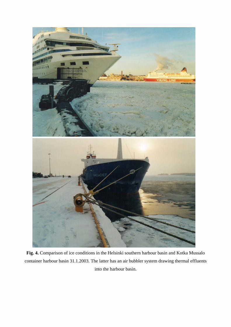
Fig. 4. Comparison of ice conditions in the Helsinki southern harbour basin and Kotka Mussalo

container harbour basin 31.1.2003. The latter has an air bubbler system drawing thermal effluents

into the harbour basin.

Fig. 5. Main mechanisms of brash ice formation.

Bubbler system, 300 meters

Sea current outflow

Sea current inflow

Fig. 6. The simulation area.

Fig. 7. Simulated bubbler flow close to the harbor bank.

Fig. 8. Flow circulations driven by the bubbler for larger regions.

Fig. 9. Bubbler’s effect on heat energy loss (W/m2), assuming the ice is rough and average water

temperature is about 0.1 C.

Table 1 Water flow rate driven by bubbler at different layers

Layer depth from

surface, m

No ice, nominal

flow 0.37 m3/s.m

Ice cover, nominal

flow 0.37 m3/s.m

Ice cover, nominal

flow 0.26 m3/s.m

11 0.071 0.073 0.052

10.21 0.112 0.111 0.079

9.43 0.149 0.147 0.105

8.64 0.186 0.181 0.129

7.86 0.220 0.214 0.153

7.07 0.253 0.244 0.174

6.29 0.284 0.272 0.194

5.5 0.312 0.297 0.213

4.71 0.337 0.319 0.228

3.93 0.357 0.338 0.241

3.14 0.373 0.349 0.249

2.36 0.375 0.347 0.248

1.57 0.343 0.312 0.223

0.78 0.237 0.207 0.148