Embed Size (px)
Citation preview
Application demonstration
BifTools
Maple Package for Bifurcation Analysis in Dynamical Systems
Milen Borisov, Neli Dimitrova
Department of Biomathematics
Institute of Mathematics and Informatics
Bulgarian Academy of Sciences, Sofia, Bulgaria
[email protected], [email protected]
Introduction
Nonlinear dynamical systems depending on parameters may have very complicated behavior when some
parameters are changed. These changes may lead to the appearance or disappearance of equilibrium points,
periodic orbits or more complicated features [6], [9]. Given a dynamical system, our ultimate goal is to
obtain its bifurcation diagram, that is to divide the parameter space into regions within which the system has
topologically equivalent phase portraits. The center manifold theory proposes a systematic way for studying
such kind of problems by simplification of the dynamical systems. Reducing a dynamical system to its
center manifold means computation of a parameter-dependent normal form for each bifurcation point in the
minimal possible phase space dimension and specification of the relevant genericity conditions. The
parameter and coordinate transformations required to put the system into the normal form lead to lengthy
intermediate calculations for manual work like symbolic Jacobian computations, Taylor series coefficients,
eigenvalues and eigenvectors computations. The Maple package BifTools is aimed to replace this tedious
manual work by faster and more rigorous computations.
This worksheet demonstrates the use of the Maple package BifTools for symbolic and numeric bifurcation
analysis of dynamical systems. The package consists of five main procedures:
BifTools [calcHopfBifPoints] calculates the Andronov-Hopf bifurcation points of an ODE system,
using the method of resultants.
BifTools [calcHopfBif] calculates the normal form of the Andronov-Hopf bifurcation of the
equilibrium points.
BifTools[calcOneZeroEigenvalueBifPoints] calculates the bifurcation points of an ODE system
with a single zero eigenvalue of the Jacobian.
BifTools [calcOneZeroEigenvalueBif] calculates the normal form of the steady states bifurcations
with a single zero eigenvalue of the Jacobian.
BifTools [calcBTBif] calculates the normal form of the Bogdanov-Takens (double zero) bifurcation,
using the projection or the direct method for center manifold reduction.
Note! Normal form reduction of the ODE system requires exact (i. e. symbolic or rational-arithmetic)
computations.
Below we present examples to demonstrate the facilities of the BifTools procedures.
Package version
Package BifTools v.1.1.1
Requirements
Software Requirements: Maple 13 or higher versions
Initialization
Restart the Maple. > restart:
Tell Maple where to find the package library BifTools.mla.
For example, in the line below, replace "/home/milen/Desktop/Maple/work/BifTools/BifTools.mla" by your
path to the BifTools.mla library file
(e.g. Linux: "/usr/maple/mylib/BifTools.mla" or Windows: "C:\\Maple\\MyLib\\BifTools.mla"); > libfile := "/home/milen/Desktop/Maple/work/BifTools/BifTools.mla":
libname := libname, libfile:
Load the package using the 'with' command: > with(BifTools):
Local One-Parameter Bifurcations of Equilibrium Points
Consider a continuous-time autonomous dynamical system:
(1) x' = f(x , α) , x ∈Rn , α∈R
1,
where f is smooth with respect to x and α. Let (x, α) = (x0 , α0) be a fixed point of the system, i. e. f(x0, α0)
= 0. The main two questions are:
1. Is the fixed point stable or unstable?
2. How is the stability or instability affected as α is varied?
The answer of the first question is simple when the fixed point (x0, α0) is hyperbolic (i. e. none of the
eigenvalues of the Jacobian matrix of f at this point lies on the imaginary axis). In this case the stability of
(x0, α0) is determined by the associated linear system
(2) x' = Dx f(x0, α0) x ,
e. g. the hyperbolic point (x0, α0) is asymptotically stable, if all eigenvalues of the Jacobian Dx f(x0, α0)
have negative real parts, and (x0, α0) is not stable, if at least one of the eigenvalues of Dx f(x0, α0) has a
positive real part. It is also known that under small variations of α the fixed point moves slightly but
remains hyperbolic [6]. So, in a neighborhood of α0 the isolated hyperbolic fixed point persists and has
always the same stability type.
If the fixed point (x0, α0) is not hyperbolic (i. e. the Jacobian of f at this point has some eigenvalues on the
imaginary axis), then varying α slightly and close to α0 causes the stability of the fixed point to change. In
this case, if the Jacobian matrix Dx f(x0, α0) has some eigenvalues with zero real part then a local
bifurcation may occur at (x0, α0); moreover,
if a unique eigenvalue is equal to zero, then this is a saddle-node bifurcation or a transcritical
bifurcation or a pitchfork bifurcation; we shall call for short each one of them one-zero-eigenvalue
bifurcation;
if a pair of eigenvalues consists of pure imaginary complex conjugate numbers (with zero real parts),
then this is a Poincare-Andronov-Hopf bifurcation, known as Hopf bifurcation.
The second question above can be answered using the center manifold theory and the method of normal
forms. The center manifold theory allows us to reduce the dimension of a given dynamical system near a
local bifurcation, while the method of normal forms simplifies the nonlinear part of
the reduced system. So the final result is a reduced and simplified dynamical system (i. e. a dynamical
system in a normal form) which is topologically equivalent to the original dynamical system [3], [6]. The
bifurcation diagrams are well known for systems in a normal form, as we shall see below.
One-zero-eigenvalue bifurcations
There are three types of one-zero-eigenvalue bifurcations: saddle-node, transcritical and pitchfork
bifurcation. Each one of them satisfies different genericity conditions; their bifurcation diagrams are also
different. Without loss of generality let us assume that (x, α) = (0, 0) is a fixed point of one-dimensional
dynamical system depending on one parameter:
(3) x' = f(x , α) , x ∈R1 , α∈R
1
Now, for (3) to undergo a one-zero-eigenvalue bifurcation at (0, 0), the following conditions should be
satisfied:
(4) f(0, 0) = 0, fx(0, 0) = 0.
These conditions guarantee that the fixed point (0, 0) is not hyperbolic.
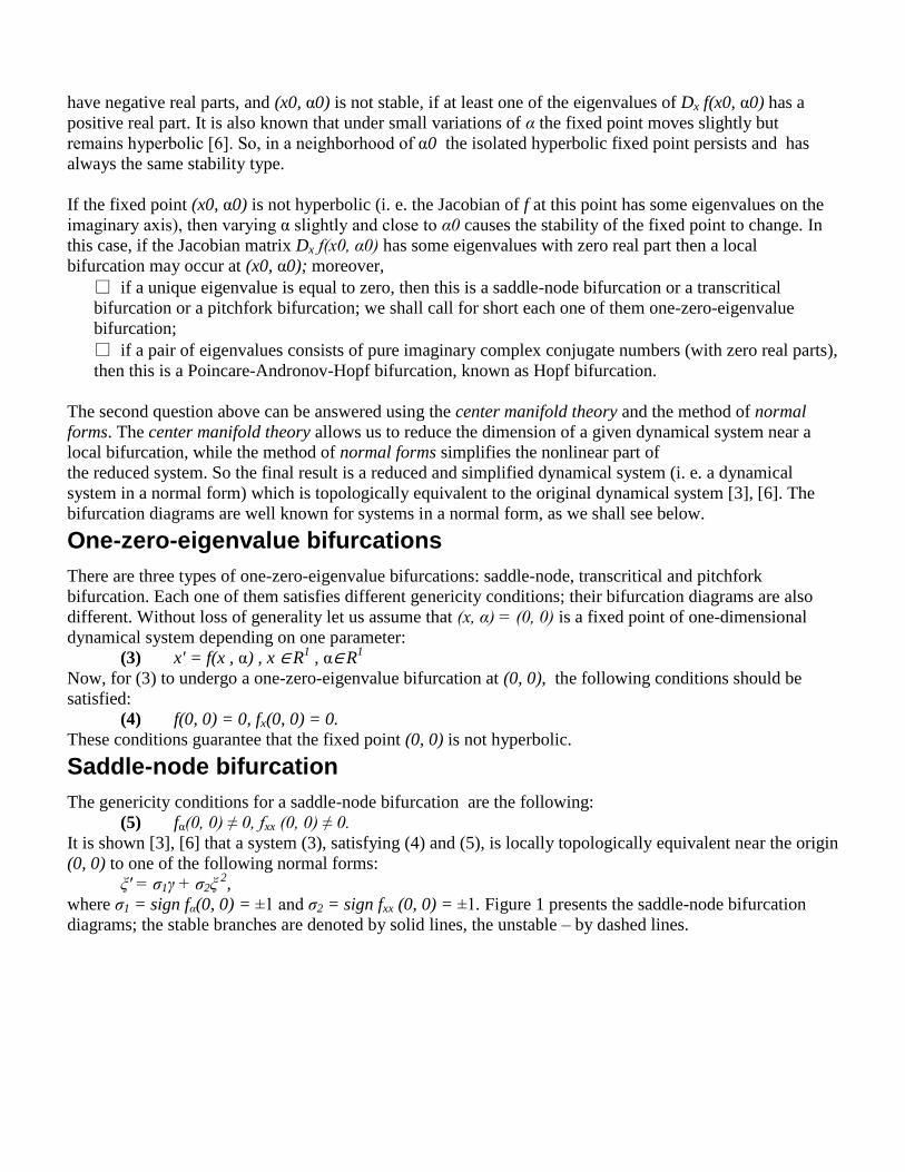
Saddle-node bifurcation
The genericity conditions for a saddle-node bifurcation are the following:
(5) fα(0, 0) ≠ 0, fxx (0, 0) ≠ 0.
It is shown [3], [6] that a system (3), satisfying (4) and (5), is locally topologically equivalent near the origin
(0, 0) to one of the following normal forms:
ξ' = σ1γ + σ2ξ 2
,
where σ1 = sign fα(0, 0) = ±1 and σ2 = sign fxx (0, 0) = ±1. Figure 1 presents the saddle-node bifurcation
diagrams; the stable branches are denoted by solid lines, the unstable – by dashed lines.
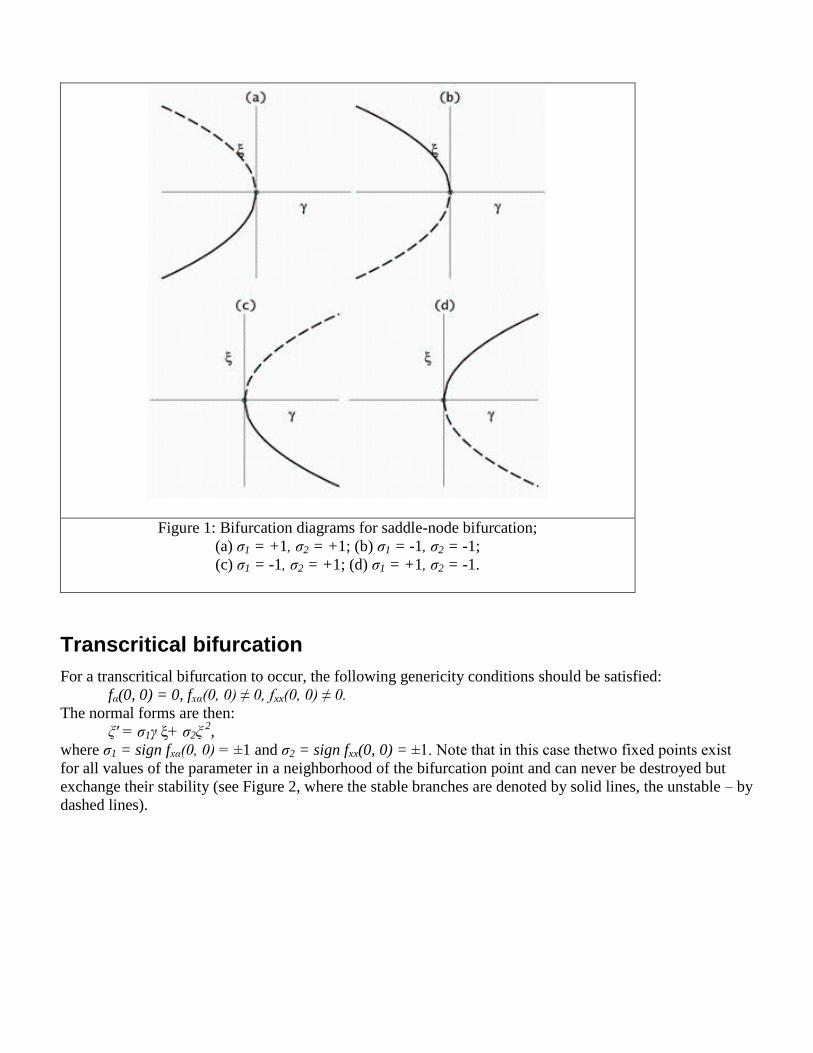
Figure 1: Bifurcation diagrams for saddle-node bifurcation;
(a) σ1 = +1, σ2 = +1; (b) σ1 = -1, σ2 = -1;
(c) σ1 = -1, σ2 = +1; (d) σ1 = +1, σ2 = -1.
Transcritical bifurcation
For a transcritical bifurcation to occur, the following genericity conditions should be satisfied:
fα(0, 0) = 0, fxα(0, 0) ≠ 0, fxx(0, 0) ≠ 0.
The normal forms are then:
ξ' = σ1γ ξ+ σ2ξ 2,
where σ1 = sign fxα(0, 0) = ±1 and σ2 = sign fxx(0, 0) = ±1. Note that in this case thetwo fixed points exist
for all values of the parameter in a neighborhood of the bifurcation point and can never be destroyed but
exchange their stability (see Figure 2, where the stable branches are denoted by solid lines, the unstable – by
dashed lines).
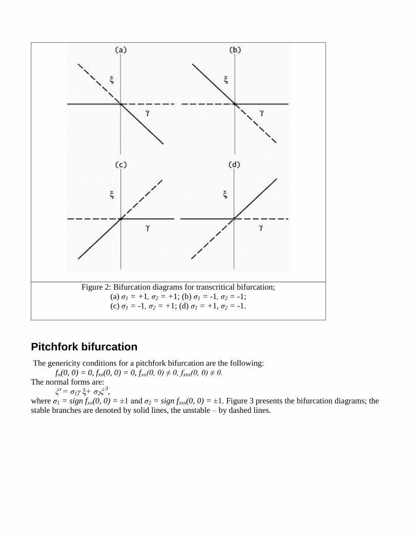
Figure 2: Bifurcation diagrams for transcritical bifurcation;
(a) σ1 = +1, σ2 = +1; (b) σ1 = -1, σ2 = -1;
(c) σ1 = -1, σ2 = +1; (d) σ1 = +1, σ2 = -1.
Pitchfork bifurcation
The genericity conditions for a pitchfork bifurcation are the following:
fα(0, 0) = 0, fxx(0, 0) = 0, fxα(0, 0) ≠ 0, fxxx(0, 0) ≠ 0.
The normal forms are:
ξ' = σ1γ ξ+ σ2ξ 3,
where σ1 = sign fxα(0, 0) = ±1 and σ2 = sign fxxx(0, 0) = ±1. Figure 3 presents the bifurcation diagrams; the
stable branches are denoted by solid lines, the unstable – by dashed lines.
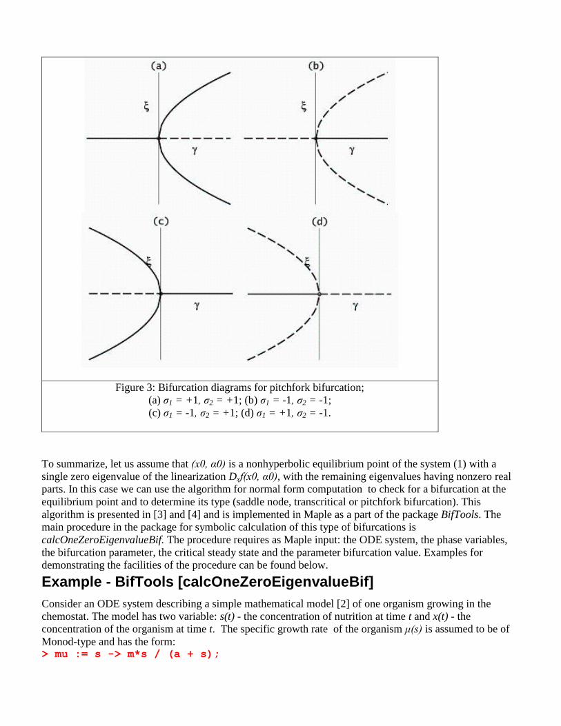
Figure 3: Bifurcation diagrams for pitchfork bifurcation;
(a) σ1 = +1, σ2 = +1; (b) σ1 = -1, σ2 = -1;
(c) σ1 = -1, σ2 = +1; (d) σ1 = +1, σ2 = -1.
To summarize, let us assume that (x0, α0) is a nonhyperbolic equilibrium point of the system (1) with a
single zero eigenvalue of the linearization Dxf(x0, α0), with the remaining eigenvalues having nonzero real
parts. In this case we can use the algorithm for normal form computation to check for a bifurcation at the
equilibrium point and to determine its type (saddle node, transcritical or pitchfork bifurcation). This
algorithm is presented in [3] and [4] and is implemented in Maple as a part of the package BifTools. The
main procedure in the package for symbolic calculation of this type of bifurcations is
calcOneZeroEigenvalueBif. The procedure requires as Maple input: the ODE system, the phase variables,
the bifurcation parameter, the critical steady state and the parameter bifurcation value. Examples for
demonstrating the facilities of the procedure can be found below.
Example - BifTools [calcOneZeroEigenvalueBif]
Consider an ODE system describing a simple mathematical model [2] of one organism growing in the
chemostat. The model has two variable: s(t) - the concentration of nutrition at time t and x(t) - the
concentration of the organism at time t. The specific growth rate of the organism μ(s) is assumed to be of
Monod-type and has the form: > mu := s -> m*s / (a + s);
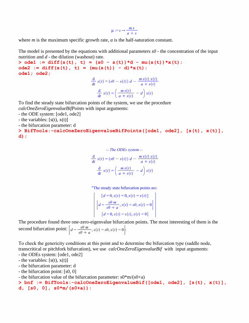
where m is the maximum specific growth rate, a is the half-saturation constant.
The model is presented by the equations with additional parameters s0 - the concentration of the input
nutrition and d - the dilution (washout) rate. > ode1 := diff(s(t), t) = (s0 - s(t))*d - mu(s(t))*x(t):
ode2 := diff(x(t), t) = (mu(s(t)) - d)*x(t):
ode1; ode2;
To find the steady state bifurcation points of the system, we use the procedure
calcOneZeroEigenvalueBifPoints with input arguments:
- the ODE system: [ode1, ode2]
- the variables: [s(t), x(t)]
- the bifurcation parameter: d > BifTools:-calcOneZeroEigenvalueBifPoints([ode1, ode2], [s(t), x(t)],
d);
The procedure found three one-zero-eigenvalue bifurcation points. The most interesting of them is the
second bifurcation point: .
Тo check the genericity conditions at this point and to determine the bifurcation type (saddle node,
transcritical or pitchfork bifurcation), we use calcOneZeroEigenvalueBif with input arguments:
- the ODEs system: [ode1, ode2]
- the variables: [s(t), x(t)]
- the bifurcation parameter: d
- the bifurcation point: [s0, 0]
- the bifurcation value of the bifurcation parameter: s0*m/(s0+a) > bnf := BifTools:-calcOneZeroEigenvalueBif([ode1, ode2], [s(t), x(t)],
d, [s0, 0], s0*m/(s0+a)):
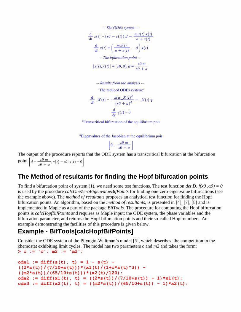
The output of the procedure reports that the ODE system has a transcritical bifurcation at the bifurcation
point .
The Method of resultants for finding the Hopf bifurcation points
To find a bifurcation point of system (1), we need some test functions. The test function det Dx f(x0 ,α0) = 0
is used by the procedure calcOneZeroEigenvalueBifPoints for finding one-zero-eigenvalue bifurcations (see
the example above). The method of resultants proposes an analytical test function for finding the Hopf
bifurcation points. An algorithm, based on the method of resultants, is presented in [4], [7], [8] and is
implemented in Maple as a part of the package BifTools. The procedure for computing the Hopf bifurcation
points is calcHopfBifPoints and requires as Maple input: the ODE system, the phase variables and the
bifurcation parameter, and returns the Hopf bifurcation points and their so-called Hopf numbers. An
example demonstrating the facilities of this procedure is given below.
Example - BifTools[calcHopfBifPoints]
Consider the ODE system of the Pilyugin-Waltman’s model [5], which describes the competition in the
chemostat exhibiting limit cycles. The model has two parameters c and m2 and takes the form: > c := 'c': m2 := 'm2':
ode1 := diff(s(t), t) = 1 - s(t) -
((2*s(t))/(7/10+s(t)))*(x1(t)/(1+c*s(t)^3)) -
((m2*s(t))/(65/10+s(t)))*(x2(t)/120):
ode2 := diff(x1(t), t) = ((2*s(t))/(7/10+s(t)) - 1)*x1(t):
ode3 := diff(x2(t), t) = ((m2*s(t))/(65/10+s(t)) - 1)*x2(t):
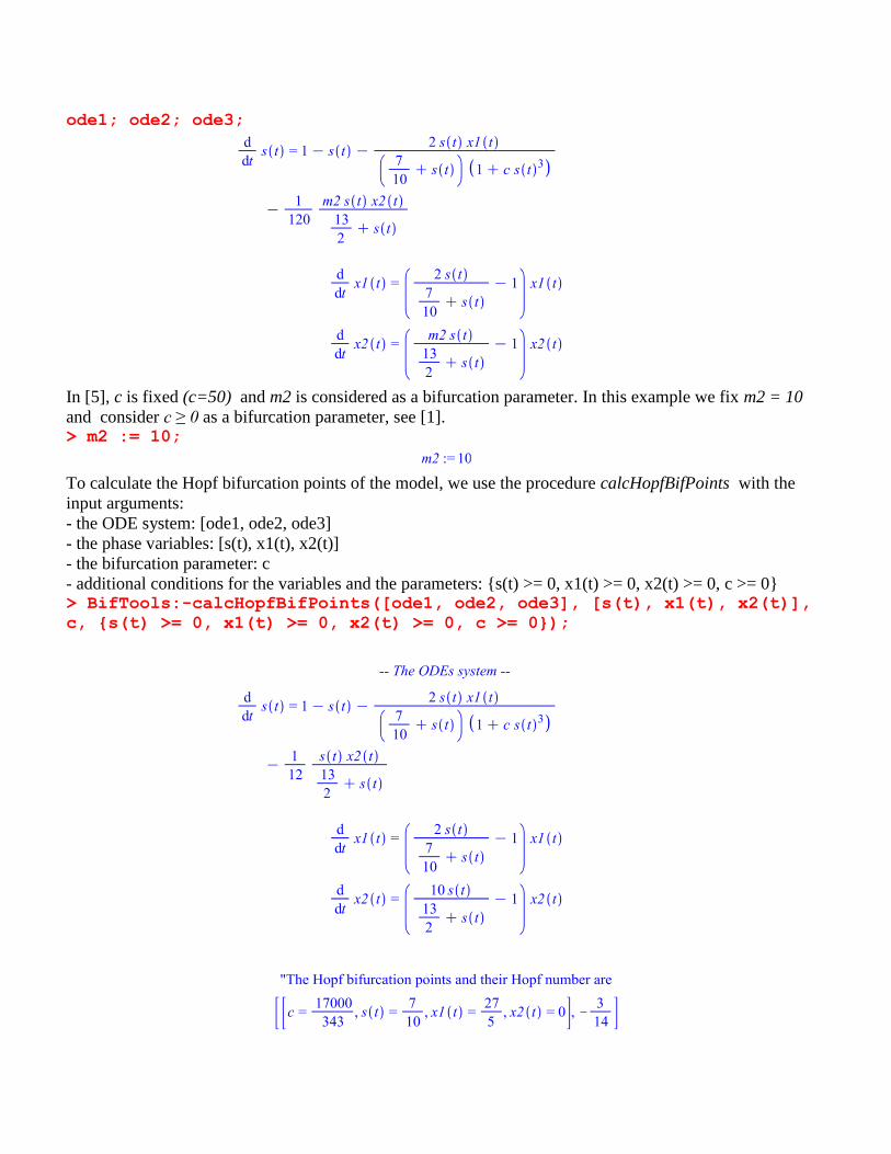
ode1; ode2; ode3;
In [5], c is fixed (c=50) and m2 is considered as a bifurcation parameter. In this example we fix m2 = 10
and consider c ≥ 0 as a bifurcation parameter, see [1]. > m2 := 10;
To calculate the Hopf bifurcation points of the model, we use the procedure calcHopfBifPoints with the
input arguments:
- the ODE system: [ode1, ode2, ode3]
- the phase variables: [s(t), x1(t), x2(t)]
- the bifurcation parameter: c
- additional conditions for the variables and the parameters: {s(t) >= 0, x1(t) >= 0, x2(t) >= 0, c >= 0} > BifTools:-calcHopfBifPoints([ode1, ode2, ode3], [s(t), x1(t), x2(t)],
c, {s(t) >= 0, x1(t) >= 0, x2(t) >= 0, c >= 0});
As a result the procedure returns one Hopf bifurcation point . In
the next example we shall calculate the Hopf bifurcation normal form of the system at this point.
Hopf Bifurcation
Again, without loss of generality let us assume that (x, α) = (0, 0) is a fixed point of the system (1). Assume
also that the linearization Dx f(0, α) of (1) has at (0, α) for sufficiently small |α| a pair of complex conjugate
eigenvalues λ1,2(α) = λR(α) ± i λI(α), where λR(0) = 0 and λI(0) > 0. If the following genericity conditions
hold true:
l1(0) ≠ 0, where l1(0) is the first Lyapunov coefficient;
λR'(0) ≠0 (transversality condition),
then the dynamics (1) is topologically equivalent near the fixed point to the normal form (see [6], [9]):
ξ' = σ0γ ξ - η + σ1(ξ2
+ η2) ξ
η' = ξ + σ0 γ η + σ1(ξ2+ η
2) η.
where σ0 = sign λR'(0) = ±1 and σ1 = sign l1(0) = ±1. The origin (0,0) is a fixed point of the normal form;
moreover, if
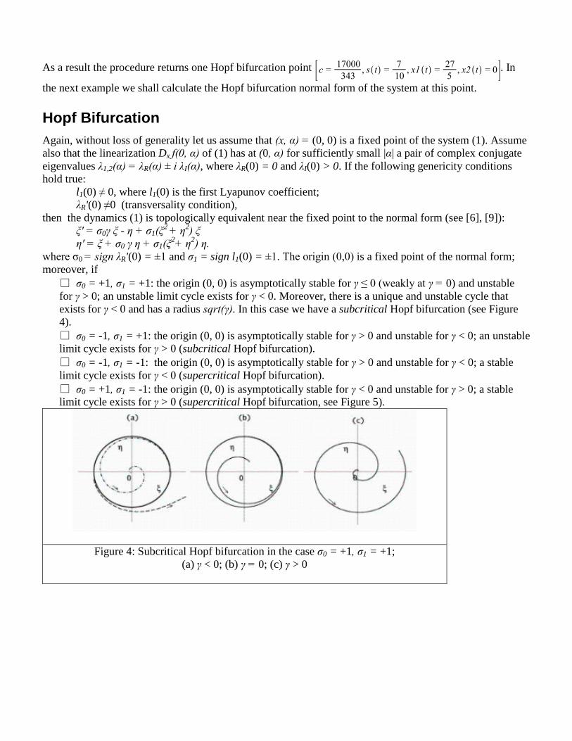
σ0 = +1, σ1 = +1: the origin (0, 0) is asymptotically stable for γ ≤ 0 (weakly at γ = 0) and unstable
for γ > 0; an unstable limit cycle exists for γ < 0. Moreover, there is a unique and unstable cycle that
exists for γ < 0 and has a radius sqrt(γ). In this case we have a subcritical Hopf bifurcation (see Figure
4).
σ0 = -1, σ1 = +1: the origin (0, 0) is asymptotically stable for γ > 0 and unstable for γ < 0; an unstable
limit cycle exists for γ > 0 (subcritical Hopf bifurcation).
σ0 = -1, σ1 = -1: the origin (0, 0) is asymptotically stable for γ > 0 and unstable for γ < 0; a stable
limit cycle exists for γ < 0 (supercritical Hopf bifurcation).
σ0 = +1, σ1 = -1: the origin (0, 0) is asymptotically stable for γ < 0 and unstable for γ > 0; a stable
limit cycle exists for γ > 0 (supercritical Hopf bifurcation, see Figure 5).
Figure 4: Subcritical Hopf bifurcation in the case σ0 = +1, σ1 = +1;
(a) γ < 0; (b) γ = 0; (c) γ > 0
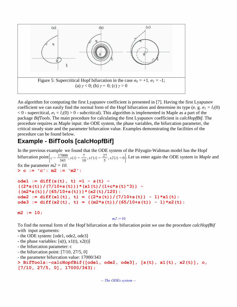
Figure 5: Supercritical Hopf bifurcation in the case σ0 = +1, σ1 = -1;
(a) γ < 0; (b) γ = 0; (c) γ > 0
An algorithm for computing the first Lyapunov coefficient is presented in [7]. Having the first Lyapunov
coefficient we can easily find the normal form of the Hopf bifurcation and determine its type (e. g. σ1 = l1(0)
< 0 - supercitical, σ1 = l1(0) > 0 - subcritical). This algorithm is implemented in Maple as a part of the
package BifTools. The main procedure for calculating the first Lyapunov coefficient is calcHopfBif. The
procedure requires as Maple input: the ODE system, the phase variables, the bifurcation parameter, the
critical steady state and the parameter bifurcation value. Examples demonstrating the facilities of the
procedure can be found below.
Example - BifTools [calcHopfBif]
In the previous example we found that the ODE system of the Pilyugin-Waltman model has the Hopf
bifurcation point . Let us enter again the ODE system in Maple and
fix the parameter m2 = 10. > c := 'c': m2 := 'm2':
ode1 := diff(s(t), t) =1 - s(t) -
((2*s(t))/(7/10+s(t)))*(x1(t)/(1+c*s(t)^3)) -
((m2*s(t))/(65/10+s(t)))*(x2(t)/120):
ode2 := diff(x1(t), t) = ((2*s(t))/(7/10+s(t)) - 1)*x1(t):
ode3 := diff(x2(t), t) = ((m2*s(t))/(65/10+s(t)) - 1)*x2(t):
m2 := 10;
To find the normal form of the Hopf bifurcation at the bifurcation point we use the procedure calcHopfBif
with input arguments:
- the ODE system: [ode1, ode2, ode3]
- the phase variables: [s(t), x1(t), x2(t)]
- the bifurcation parameter: c
- the bifurcation point: [7/10, 27/5, 0]
- the parameter bifurcation value: 17000/343 > BifTools:-calcHopfBif([ode1, ode2, ode3], [s(t), x1(t), x2(t)], c,
[7/10, 27/5, 0], 17000/343);
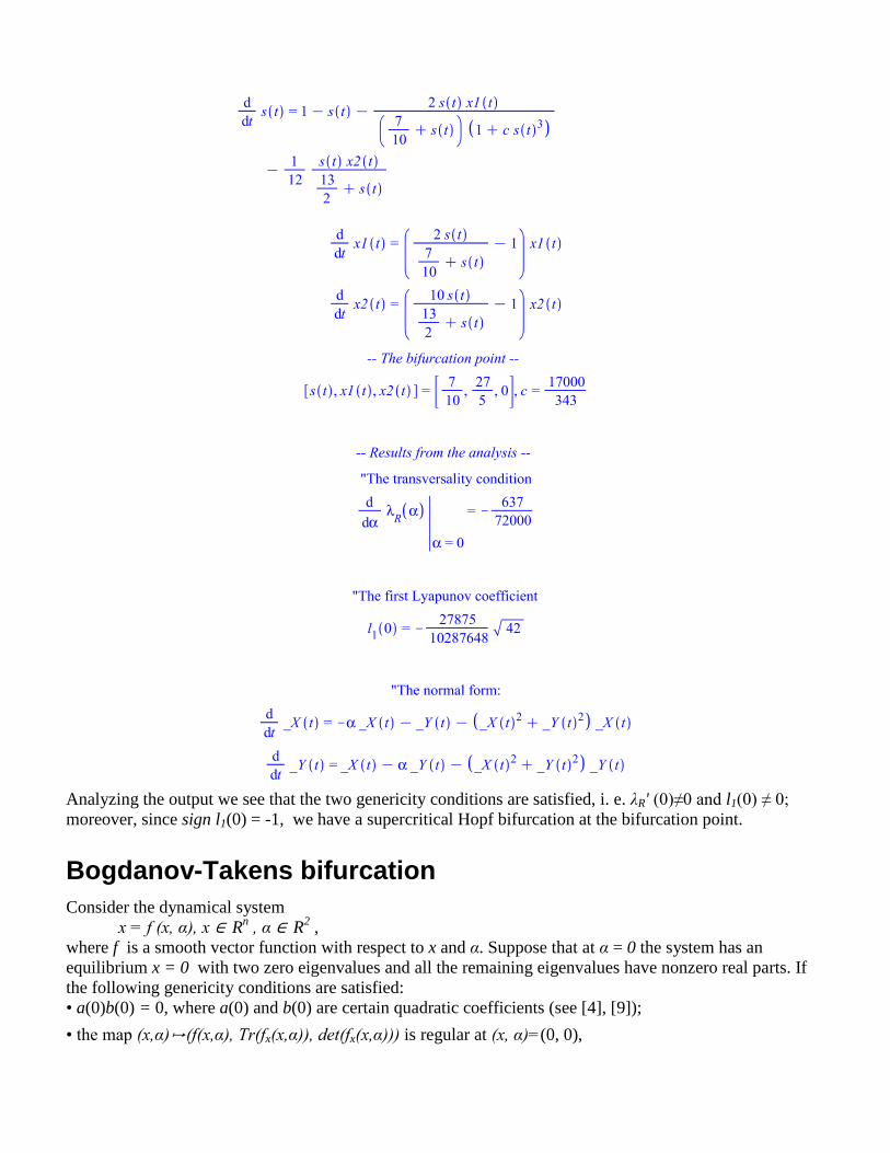
Analyzing the output we see that the two genericity conditions are satisfied, i. e. λR' (0)≠0 and l1(0) ≠ 0;
moreover, since sign l1(0) = -1, we have a supercritical Hopf bifurcation at the bifurcation point.
Bogdanov-Takens bifurcation
Consider the dynamical system
x = f (x, α), x ∈ Rn , α ∈ R
2 ,
where f is a smooth vector function with respect to x and α. Suppose that at α = 0 the system has an
equilibrium x = 0 with two zero eigenvalues and all the remaining eigenvalues have nonzero real parts. If
the following genericity conditions are satisfied:
• a(0)b(0) = 0, where a(0) and b(0) are certain quadratic coefficients (see [4], [9]);
• the map (x,α)↦(f(x,α), Tr(fx(x,α)), det(fx(x,α))) is regular at (x, α)=(0, 0),
then the system is locally topologically equivalent to the normal form:
η1' = η2,
η2' = β1+ β2η1+ η12+ ση1η2,
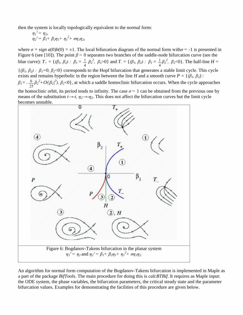
where σ = sign a(0)b(0) = ±1. The local bifurcation diagram of the normal form withσ = -1 is presented in
Figure 6 (see [10]). The point β = 0 separates two branches of the saddle-node bifurcation curve (see the
blue curve): T+ = {(β1, β2) : β1 = β22, β2>0} and T- = {(β1, β2) : β1 = β2
2, β2<0}. The half-line H =
{(β1, β2) : β1=0, β2<0} corresponds to the Hopf bifurcation that generates a stable limit cycle. This cycle
exists and remains hyperbolic in the region between the line H and a smooth curve P = {(β1, β2) :
β1= β22+O(|β2|
3), β2<0}, at which a saddle homoclinic bifurcation occurs. When the cycle approaches
the homoclinic orbit, its period tends to infinity. The case σ = 1 can be obtained from the previous one by
means of the substitution t→-t, η2→-η2. This does not affect the bifurcation curves but the limit cycle
becomes unstable.
Figure 6: Bogdanov-Takens bifurcation in the planar system
η1' = η2 and η2' = β1+ β2η1+ η12+ ση1η2.
An algorithm for normal form computation of the Bogdanov-Takens bifurcation is implemented in Maple as
a part of the package BifTools. The main procedure for doing this is calcBTBif. It requires as Maple input:
the ODE system, the phase variables, the bifurcation parameters, the critical steady state and the parameter
bifurcation values. Examples for demonstrating the facilities of this procedure are given below.
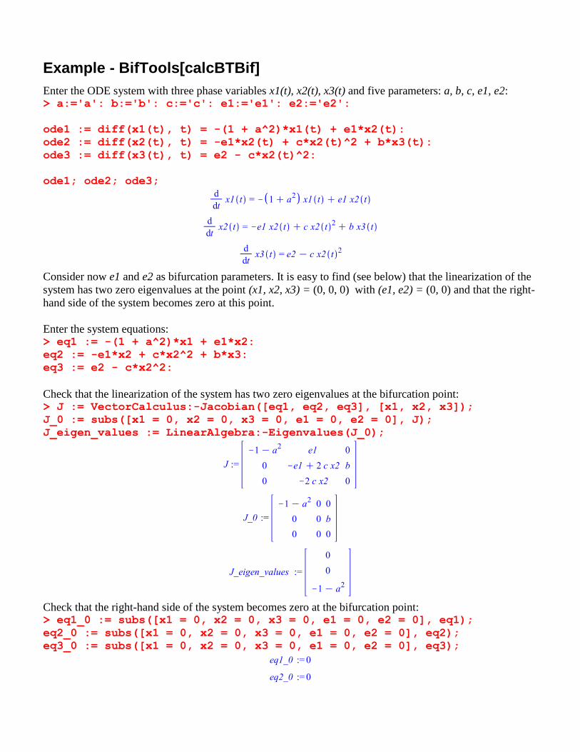
Example - BifTools[calcBTBif]
Enter the ODE system with three phase variables x1(t), x2(t), x3(t) and five parameters: a, b, c, e1, e2: > a:='a': b:='b': c:='c': e1:='e1': e2:='e2':
ode1 := diff(x1(t), t) = -(1 + a^2)*x1(t) + e1*x2(t):
ode2 := diff(x2(t), t) = -e1*x2(t) + c*x2(t)^2 + b*x3(t):
ode3 := diff(x3(t), t) = e2 - c*x2(t)^2:
ode1; ode2; ode3;
Consider now e1 and e2 as bifurcation parameters. It is easy to find (see below) that the linearization of the
system has two zero eigenvalues at the point (x1, x2, x3) = (0, 0, 0) with (e1, e2) = (0, 0) and that the right-
hand side of the system becomes zero at this point.
Enter the system equations: > eq1 := -(1 + a^2)*x1 + e1*x2:
eq2 := -e1*x2 + c*x2^2 + b*x3:
eq3 := e2 - c*x2^2:
Check that the linearization of the system has two zero eigenvalues at the bifurcation point: > J := VectorCalculus:-Jacobian([eq1, eq2, eq3], [x1, x2, x3]);
J_0 := subs([x1 = 0, x2 = 0, x3 = 0, e1 = 0, e2 = 0], J);
J_eigen_values := LinearAlgebra:-Eigenvalues(J_0);
Check that the right-hand side of the system becomes zero at the bifurcation point: > eq1_0 := subs([x1 = 0, x2 = 0, x3 = 0, e1 = 0, e2 = 0], eq1);
eq2_0 := subs([x1 = 0, x2 = 0, x3 = 0, e1 = 0, e2 = 0], eq2);
eq3_0 := subs([x1 = 0, x2 = 0, x3 = 0, e1 = 0, e2 = 0], eq3);
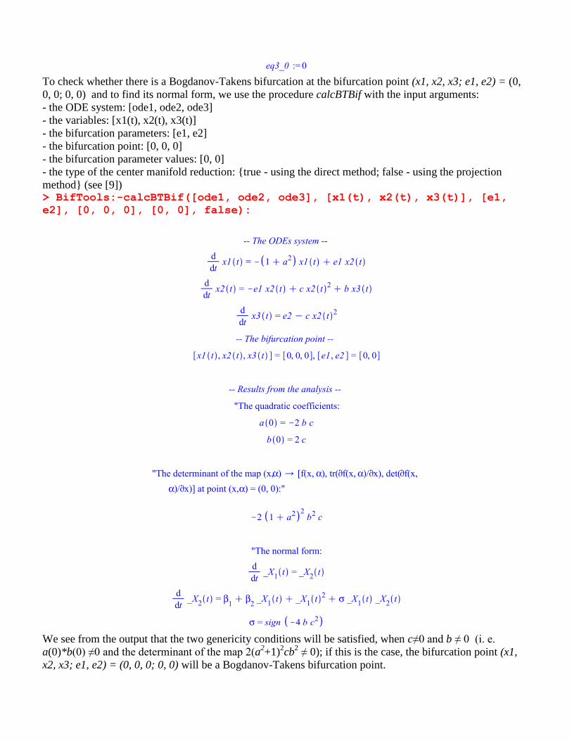
To check whether there is a Bogdanov-Takens bifurcation at the bifurcation point (x1, x2, x3; e1, e2) = (0,
0, 0; 0, 0) and to find its normal form, we use the procedure calcBTBif with the input arguments:
- the ODE system: [ode1, ode2, ode3]
- the variables: [x1(t), x2(t), x3(t)]
- the bifurcation parameters: [e1, e2]
- the bifurcation point: [0, 0, 0]
- the bifurcation parameter values: [0, 0]
- the type of the center manifold reduction: {true - using the direct method; false - using the projection
method} (see [9]) > BifTools:-calcBTBif([ode1, ode2, ode3], [x1(t), x2(t), x3(t)], [e1,
e2], [0, 0, 0], [0, 0], false):
We see from the output that the two genericity conditions will be satisfied, when c≠0 and b ≠ 0 (i. e.
a(0)*b(0) ≠0 and the determinant of the map 2(a2+1)
2cb
2 ≠ 0); if this is the case, the bifurcation point (x1,
x2, x3; e1, e2) = (0, 0, 0; 0, 0) will be a Bogdanov-Takens bifurcation point.
>
Conclusions
In this worksheet we have demonstrated the facilities of the Maple package BifTools for bifurcation analysis
of dynamical systems, examining some examples. We would highly appreciate your comments about your
own experiences using BifTools. Please send your feedback to [email protected] or [email protected].
References
[1] F. Mazenc, T. Ari, Global Dynamics of the Chemostat with Different Removal Rates and Variable
Yields, Mathematical Biosciences and Engineering, Vol. 8, No. 3, July 2011, 827–840.
[2] H. L. Smith, P. Waltman : The Theory of the Chemostat. Dynamics of Microbial Competition.
Cambridge University Press, 1995
[3] M. Borisov, N. Dimitrova, One-Parameter Bifurcation Analysis of Dynamical Systems Using Maple.
Serdica Journal of Computing, Vol. 4, Nr. 1, 2010, 43-56.
[4] M. Borisov, BifTools: Maple Package for Bifurcation Analysis of Dynamical Systems, submitted for
publication (2012).
[5] S. Pilyugin, P. Waltman, Multiple limit cycles in the chemostat with variable yields. Mathematical
Biosciences 182, (2003), 151-166.
[6] S. Wiggins, Introduction to applied nonlinear dynamical systems and chaos. Texts in Applied
Mathematics, Vol. 2, Springer, New York, eidelberg, Berlin, 1990.
[7] T. Gross, Population Dynamics: General Results from Local Analysis. PhD Thesis, Faculty of
Mathematics and Natural Sciences, Carl von ssietzky Univ. , Oldenburg, Germany, 2004.
[8] T. Gross, U. Feudel, Analytical Search for Bifurcation Surfaces in Parameter Space. Physica D 195.
[9] Y. A. Kuznetsov, Elements of applied bifurcation theory. Applied Mathematical Science 112, Springer,
New York, Heidelberg, Berlin, 1995. (2004) 292-302.
[10] Y. A. Kuznetsov, J. Guckenheimer (2007), Scholarpedia, 2(1):1854,
http://www.scholarpedia.org/article/Bogdanov-Takens_bifurcation (December 5, 2011)
See Also
For more information about:
- the package BifTools, see [3], [4] and the Readme.txt file in the package distribution
BifTools_ver.x.x.x_.zip;
- the bifurcation analysis, see [6], [9];
- the method of resultants for finding bifurcation equilibrium points, see [7], [8];
- the chemostat and biological models, see [1], [2], [5]
Legal Notice: © Maplesoft, a division of Waterloo Maple Inc. 2009. Maplesoft and Maple are trademarks
of Waterloo Maple Inc. Neither Maplesoft nor the authors are responsible for any errors contained within
and are not liable for any damages resulting from the use of this material. This application is intended for
non-commercial, non-profit use only. Contact the authors for permission if you wish to use this application
in for-profit activities.