Application of Artificial Neural Network and Support Vector … · Support Vector Regression in Cognitive Radio Networks for RF Power Prediction Using Compact Differential Evolution

Application of Artificial Neural Network and

Support Vector Regression in Cognitive Radio

Networks for RF Power Prediction Using Compact

Differential Evolution AlgorithmSunday Iliya, Eric Goodyer, John Gow, Jethro Shell and Mario Gongora

Centre for Computational Intelligence,

School of Computer Science and Informatics,

De Montfort University, The Gateway,

Leicester LE1 9BH, England, United Kingdom

Email: [email protected], [email protected], [email protected]

[email protected], [email protected]

Abstract—Cognitive radio (CR) technology has emerged as apromising solution to many wireless communication problemsincluding spectrum scarcity and underutilization. To enhancethe selection of channel with less noise among the white spaces(idle channels), the a priory knowledge of Radio Frequency(RF) power is very important. Computational Intelligence (CI)techniques cans be applied to these scenarios to predict therequired RF power in the available channels to achieve optimumQuality of Service (QoS). In this paper, we developed a timedomain based optimized Artificial Neural Network (ANN) andSupport Vector Regression (SVR) models for the prediction ofreal world RF power within the GSM 900, Very High Frequency(VHF) and Ultra High Frequency (UHF) FM and TV bands.Sensitivity analysis was used to reduce the input vector of theprediction models. The inputs of the ANN and SVR consist ofonly time domain data and past RF power without using any RFpower related parameters, thus forming a nonlinear time seriesprediction model. The application of the models produced wasfound to increase the robustness of CR applications, specificallywhere the CR had no prior knowledge of the RF power relatedparameters such as signal to noise ratio, bandwidth and biterror rate. Since CR are embedded communication devices withmemory constrain limitation, the models used, implemented anovel and innovative initial weight optimization of the ANN’sthrough the use of compact differential evolutionary (cDE)algorithm variants which are memory efficient. This was foundto enhance the accuracy and generalization of the ANN model.

Index Terms—Cognitive Radio; Primary User; Artificial Neu-ral Network; Support Vector Machine; Compact DifferentialEvolution; RF Power; Prediction.

I. INTRODUCTION

DUE TO the current static spectrum allocation policy,

most of the licensed radio spectrum are not maximally

utilized and often free (idle) while the unlicensed spectrum are

overcrowded. Hence the current spectrum scarcity is the direct

consequence of static spectrum allocation policy and not the

fundamental lack of spectrum. The first bands to be approved

for CR communication by the US Federal Communication

Commission (FCC) because of their gross underutilization in

time, frequency and spatial domain are the very high frequency

and ultra-high frequency (VHF/UHF) TV bands [1] [2] [3]. In

this paper, we focused on the study of real world RF power

distribution in some selected channels (54MHz to 110MHz,

470MHz to 670MHz, 890MHz to 908.3MHz GSM up-link,

935MHz to 953.3MHz GSM down-link) within the VHF/UHF

bands, FM band, and the GSM 900 band. The problem of

spectrum scarcity and underutilization, can be minimized by

adopting a new paradigm of wireless communication scheme.

Advanced Cognitive Radio (CR) network or Adaptive Spec-

trum Sharing (ASS) is one of the ways to optimize our wireless

communications technologies for high data rates in a dynamic

environment while maintaining user desired quality of service

(QoS) requirements. CR is a radio equipped with the capability

of awareness, perception, adaptation and learning of its radio

frequency (RF) environment [4]. CR is an intelligent radio

where many of the digital signal processing that were tradi-

tionally done in static hardware are implemented via software.

Irrespective of the definition of CR, it has the followings

basic features: observation, adaptability and intelligence. CR

is the key enabling tool for dynamic spectrum access and

a promising solution for the present problem of spectrum

scarcity and underutilization. Cognitive radio network is made

up of two users i.e. the license owners called the primary users

(PU) who are the incumbent legitimate owners of the spectrum

and the cognitive radio commonly called the secondary users

(SU) who intelligently and opportunistically access the unused

licensed spectrum based on some agreed conditions. CR access

to licensed spectrum is subject to two constrains i.e on no

interference base, this implies that CR can use the licensed

spectrum only when the licensed owners are not using the

channel (the overlay CR scheme). The second constrain is on

the transmitted power, in this case, SU can coexist with the PU

as long as the interference to the PU is below a given threshold

which will not be harmful to the PU nor degrade the QoS

requirements of the PU (the underlay CR network scheme)

[5] [1]. There are four major steps involved in cognitive

radio network, these are: spectrum sensing, spectrum decision,

spectrum sharing, and spectrum mobility [6] [7].

Proceedings of the Federated Conference on

Computer Science and Information Systems pp. 55–66

DOI: 10.15439/2015F14

ACSIS, Vol. 5

978-83-60810-66-8/$25.00 c©2015, IEEE 55

In spectrum sensing, the CR senses the PU spectrumusing either energy detector, cyclostationary features detector,cooperative sensing, match filter detector, eigenvalue detector,etc to sense the occupancy status of the PU [8]. Based on thesensing results, the CR will take a decision using a binaryclassifier to classify the PU channels (spectrum) as eitherbusy or idle there by identifying the white spaces (spectrumholes or idle channels). Spectrum sharing deals with efficientallocation of the available white spaces to the CR (SU) withina given geographical location at a given period of time whilespectrum mobility is the ability of the CR to vacate thechannels when the PU reclaimed ownership of the channel andsearch for another spectrum hole to communicate. During thewithdrawal or search period, the CR should maintain seamlesscommunication. Many wireless broadband devices rangingfrom simple communication to complex systems automation,are deployed daily with increasing demand for more, this callsfor optimum utilization of the limited spectrum resources viaCR paradigm. Future wireless communication device shouldbe enhanced with cognitive capability for optimum spectrumutilization. CRs are embedded wireless communication deviceswith limited memory, thus in this paper, we utilized the powerof compact differential evolutionary (cDE) algorithm whichis memory efficient, to develop an optimized ANN and SVRmodel for the prediction of real world radio frequency (RF)power. RF power traffics is a function of time, geographicallocation (longitude and latitude), height above the sea level(altitude) and the frequency or channels properties. Since ourexperiment is conducted at a fixed geographical location andat constant height, the inputs of the ANN and SVR consist ofonly past RF power samples, current time domain informationand frequency (channel) while the output is the predictedcurrent RF power in decibel (dB) (i.e. the current RF power ismodelled as a function of time, frequency and past RF powersamples) hence forming a nonlinear time series predictionmodel. ANN and SVR models were adopted because of thedynamic nonlinearity often associated with RF traffic pattern,coupled with random interfering signals or noise resultingfrom both artificial and natural sources. The use of sensitivityanalysis as detailed in Section VIII for the determinationof the optimum number of past recent RF power samplesto be used as part of the input of the ANN or SVR forprediction of current RF power, results into a more compact,robust, accurate, and well generalized models. The proposedalgorithm used a priori data to enable the system to avoidnoisy channels. The prior knowledge of the RF power allowedthe cognitive radio to predictively select channels with theleast noise among those that were unused or free. This wouldallow for a reduced utilization of radio resources includingtransmitted power, bandwidth, and in turn maximizing theusage of the limited spectrum resources. The data used inthis study was obtained by capturing real world RF datafor two months using Universal Software Radio Peripheral1 (USRP 1). The digital signal processing and capturing ofthe data were done using gnuradio which is a combinationof Python for scripting and C++ for signal processing blocks;while the models design and prediction were done in Matlab.The experiment was conducted at Centre for ComputationalIntelligence, De Montfort University, UK, located very closeto Leicester city centre.

Many prediction models used in CR radio uses known RF

related parameters as their inputs of which licensed ownerswill not be willing to dispose such information to CR users.Some of the models are based on explicit mathematical modelwhich may be different from real world situation as highlightedin Section II. Some of the prediction models aim at predictionof spectrum holes, but the fact that spectrum holes (vacantchannels) are known does not depict any information aboutthe best channel to be used among the idle channels as thenoise level is not flat for all the channels. Thus the majorcontribution of our model is that it can be used for Rf powerprediction where the CR has no prior knowledge of any RFpower related parameter. This will enable the CR to avoidnoisy channels. The model is trained and tested using realworld data. Also instead of training the ANN using backpropagation algorithms (BPA) which often lack optimality dueto premature convergent, the weights of the ANN are initiallyevolves using cDE and then fine tune using BPA, this wasfound to produce a more accurate and generalized model ascompared with the one trained using only BPA. SVR was alsoexamined using different kernels and we come up with themodel that is more appropriate for our studied location.

The rest of this paper is consist of the following sections.Section II consist of previously presented related research inthis field. This will be followed by Section III and SectionV, that gives brief description of neural network and theoptimization algorithms implemented. Experimental details arediscussed in Section VII. The paper is concluded with SectionIX, which discusses the results of the experiments, Section Xgives the summary of the findings.

II. RELATED WORK

There are different types and variants of ComputationalIntelligence (CI) and machine learning algorithms that can beused in CR such as genetic algorithms for optimization oftransmission parameters [9], swarm intelligence for optimiza-tion of radio resource allocation [10], fuzzy logic system (FLS)for decision making [11] [12], neural network and hiddenMarkov model for prediction of spectrum holes; game theory,linear regression and linear predictors for spectrum occupancyprediction [13] , Bayesian inference based predictors, etc.Some of the CI methods are used for learning and prediction,some for optimization of certain transmission parameters whileothers for decision making [14]. TV idle channels predictionusing ANN was proposed in [15], however, data were collectedonly for two hours everyday day (5pm to 7pm) within a periodof four weeks, this is not sufficient to capture all the varioustrends associated with TV broadcast. Also, identifying the idlechannels does not depict any spatial or temporal informationof the expected noise and/ or level of interference based onthe channels history which is vital in selecting the channels tobe used among the idle channels. Spectrum hole predictionusing Elman recurrent artificial neural network (ERANN)was proposed in [16]. It uses the cyclostationary featuresof modulated signals to determine the presence or absenceof primary signals while the input of the ERANN consistsof time instances. The inputs and the target output used inthe training of the ERANN and prediction were modelledusing ideal multivariate time series equations, which are oftendifferent from real life RF traffics where PU signals can beembedded in noise and/ or interfering signals. Traffic pattern

56 PROCEEDINGS OF THE FEDCSIS. ŁODZ, 2015

prediction using seasonal autoregressive integrated moving-average (SARIMA) was proposed for reduction of CRs hop-ping rate and interference effects on PU while maintaining afare blocking rate [17]. The model (SARIMA) does not depictany information about the expected noise power.

Fuzzy logic (FL) is a CI method that can capture andrepresent uncertainty. As a result it has been used in CRresearch for decision making processes. In [11] an FL baseddecision-making system with a learning mechanism was devel-oped for selection of optimum spectrum sensing techniques fora given band. Among these techniques are matched filtering,correlation detection, features detection, energy detection, andcooperative sensing. Adaptive neural fuzzy inference system(ANFIS) was used for prediction of transmission rate [18].This model was designed to predict the data rate (6, 12, 24,36, 48 and 54 Mbps) that can be achieved in wireless local areanetwork (WLAN) using a 802.11a/g configuration as a functionof time. The training data set was obtained by generating arandom data rate with an assigned probability of occurrenceat a given time instance, thus forming a time series. In thisstudy, real world RF data wasn’t used. More importantly, theresearch did not take into account the dynamic nature of noiseor interference level which can affect the predicted data rates.Semi Markov model (SMM) and continuous-time Markovchain (CTMC) models have also been used for the predictionof packet transmission rates [19]. This avoids packet collisionsthrough spectrum sensing and prediction of temporal WLANactivities combined with hoping to a temporary idle channel.However, SMM are not memory efficient, neither was there anyreference made to the expected noise level among the inactive(idle) channels to be selected. An FL based decision systemwas modeled for spectrum hand-off decision-making in a con-text characterized by uncertain and heterogeneous information[12] and fuzzy logic transmit power control for cognitiveradio. The proposed system was used for the minimizationof interference to PU’s while ensuring the transmission rateand quality of service requirements of secondary users [20].The researcher did not, however, include any learning frompast experience or historical data. An exponential movingaverage (EMA) spectrum sensing using energy prediction wasimplemented in [21]. The EMA achieved a prediction averagemean square error (MSE) of 0.2436 with the assumption thatthe channel utilization follow exponential distribution with rateparameter λ = 0.2 and signal to noise (SNR) of 10dB; RF realworld data was not used in their study. Within this paper wedemonstrate the use of SVR and an ANN trained using cDEfor prediction of real world RF power of selected channelswithin the GSM band, VHF and UHF bands. An optimizedANN model was produced by combining the global searchcapabilities of cDE algorithm variants and the local searchadvantages of back-propagation algorithms (BPA). The initialweights of the ANN were evolved using cDE after whichthe ANN was trained (fine tune) more accurately using back-propagation algorithms. This methodology demonstrates theapplication of previously acquired real world data to enhancethe prediction of RF power to assist the implementation of CRapplications. The meta parameters that govern the accuracy andgeneralization SVR model were evolves using cDE.

III. ARTIFICIAL NEURAL NETWORK

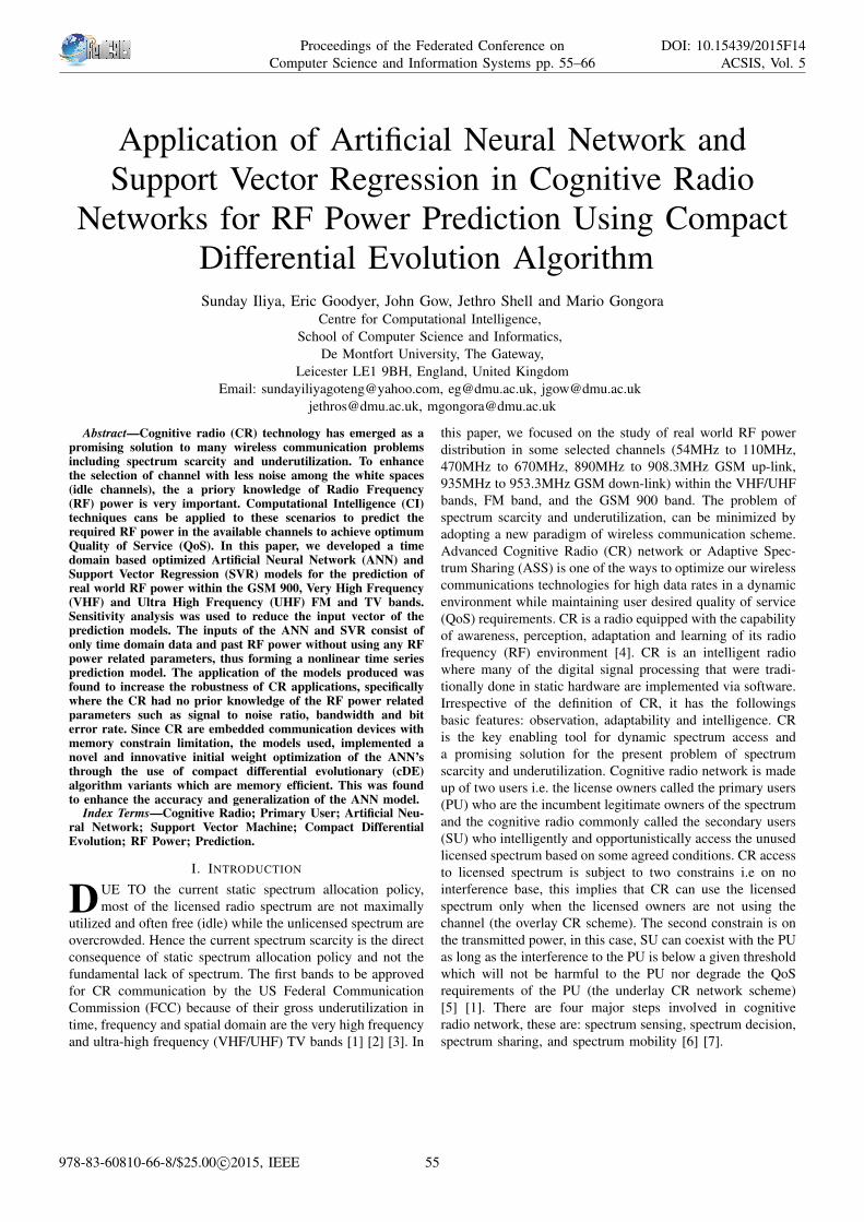
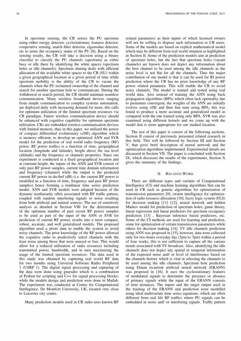
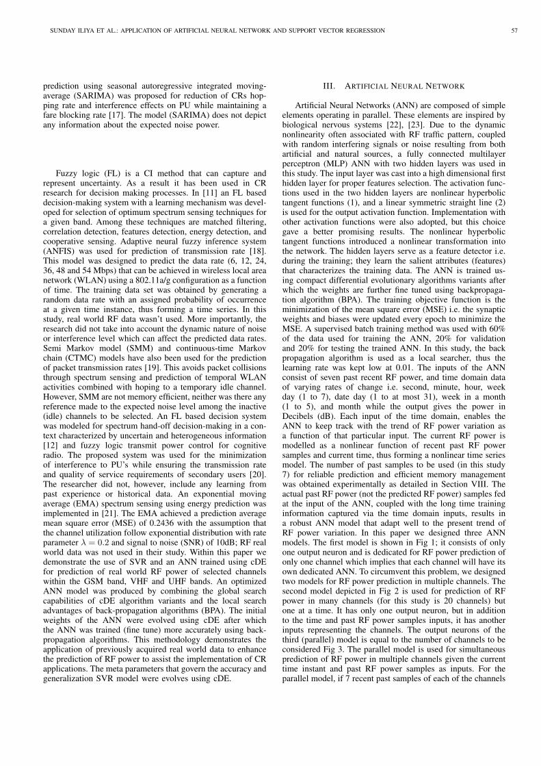
Artificial Neural Networks (ANN) are composed of simpleelements operating in parallel. These elements are inspired bybiological nervous systems [22], [23]. Due to the dynamicnonlinearity often associated with RF traffic pattern, coupledwith random interfering signals or noise resulting from bothartificial and natural sources, a fully connected multilayerperceptron (MLP) ANN with two hidden layers was used inthis study. The input layer was cast into a high dimensional firsthidden layer for proper features selection. The activation func-tions used in the two hidden layers are nonlinear hyperbolictangent functions (1), and a linear symmetric straight line (2)is used for the output activation function. Implementation withother activation functions were also adopted, but this choicegave a better promising results. The nonlinear hyperbolictangent functions introduced a nonlinear transformation intothe network. The hidden layers serve as a feature detector i.e.during the training; they learn the salient attributes (features)that characterizes the training data. The ANN is trained us-ing compact differential evolutionary algorithms variants afterwhich the weights are further fine tuned using backpropaga-tion algorithm (BPA). The training objective function is theminimization of the mean square error (MSE) i.e. the synapticweights and biases were updated every epoch to minimize theMSE. A supervised batch training method was used with 60%of the data used for training the ANN, 20% for validationand 20% for testing the trained ANN. In this study, the backpropagation algorithm is used as a local searcher, thus thelearning rate was kept low at 0.01. The inputs of the ANNconsist of seven past recent RF power, and time domain dataof varying rates of change i.e. second, minute, hour, weekday (1 to 7), date day (1 to at most 31), week in a month(1 to 5), and month while the output gives the power inDecibels (dB). Each input of the time domain, enables theANN to keep track with the trend of RF power variation asa function of that particular input. The current RF power ismodelled as a nonlinear function of recent past RF powersamples and current time, thus forming a nonlinear time seriesmodel. The number of past samples to be used (in this study7) for reliable prediction and efficient memory managementwas obtained experimentally as detailed in Section VIII. Theactual past RF power (not the predicted RF power) samples fedat the input of the ANN, coupled with the long time traininginformation captured via the time domain inputs, results ina robust ANN model that adapt well to the present trend ofRF power variation. In this paper we designed three ANNmodels. The first model is shown in Fig 1; it consists of onlyone output neuron and is dedicated for RF power prediction ofonly one channel which implies that each channel will have itsown dedicated ANN. To circumvent this problem, we designedtwo models for RF power prediction in multiple channels. Thesecond model depicted in Fig 2 is used for prediction of RFpower in many channels (for this study is 20 channels) butone at a time. It has only one output neuron, but in additionto the time and past RF power samples inputs, it has anotherinputs representing the channels. The output neurons of thethird (parallel) model is equal to the number of channels to beconsidered Fig 3. The parallel model is used for simultaneousprediction of RF power in multiple channels given the currenttime instant and past RF power samples as inputs. For theparallel model, if 7 recent past samples of each of the channels

SUNDAY ILIYA ET AL.: APPLICATION OF ARTIFICIAL NEURAL NETWORK AND SUPPORT VECTOR REGRESSION 57

were used as distinct feedback inputs, there will be a total of7N feedback inputs; where N is the number of channels Fig 3;and the training will be computationally expensive. These largefeedback inputs ware reduced to 7 by using their average.Thedata used in this study were obtained by capturing real worldRF signals within the GSM 900, VHF and UHV TV and FMbands for a period of two months. In all the models, no RFpower related parameters such as signal to noise ratio (SNR),bandwidth, and modulation type, are used as the input ofthe ANN. Thus making the models robust for cognitive radioapplication where the CR has no prior knowledge of these RFpower related parameters.

Artificial neural network architecture can be broadly clas-sified as either feed forward or recurrent type [22]. Each ofthese two classes can be structured in different configurations.A feed forward network is one in which the output of onelayer is connected to input of the next layer via a synapticweight, while the recurrent type may have at least one feedbackconnection or connections between neurons within the samelayer or other layers depending on the topology (architecture).The training time of the feed forward is less compared to thatof the recurrent type but the recurrent type has better memorycapability for recalling past events. Four ANN topologieswere considered: feed forward (FF), cascaded feed forward(CFF), feed forward with output feedback (FFB), and layeredrecurrent (LR) ANN.

The accuracy and level of generalization of ANN dependlargely on the initial weights and biases, learning rate, mo-mentum constant,training data and also the network topology.In this paper, the learning rate and the momentum werekept constant at 0.01 and 0.008 respectively while the initialweights and biases were evolved using compact differentialevolutionary algorithm variants. The first generation initialweights and biases were randomly generated and constrainedwithin the decision space of -2 to 2. After 1000 generations,the ANN weights and biases were initialized using the elite i.e.the most fittest solution (candidate with the least MSE, obtainusing test data) and then train further using backpropagationalgorithm (BPA) to fine tune the weights as detailed in thetraining Section VI-A. Thus producing the final optimizedANN model.

F (x) = b · tanh(ax) = b(eax − e−ax

eax + e−ax) (1)

F (x) = mx+ c (2)

Where the intercept c = 0 and the gradient m is left at Matlabdefault while the constants a and b are assigned the value 1.

IV. SUPPORT VECTOR MACHINE

Support vector machine (SVM) used for regression isoften known as support vector regression (SVR). In SVR,the input space x is first mapped onto a high m dimensionalfeature space by means of certain non-linear transformation(mapping), after which a linear model f(x,w) is constructedin the feature space as shown in (4), [22]. Many time seriesregression prediction models uses certain lost functions duringthe training phase for minimization of the empirical risk,among these loss functions are mean square error, square error

Fig. 1: Dedicated ANN model for one channel

Fig. 2: Multiple channels, single output ANN model

Fig. 3: Multiple channels, parallel outputs ANN model

Where n is a time index, P (n− 1), P (n− 2), · · · , P (n− q)are the past q RF power samples while P (n) is the currentpredicted RF power.

and absolute error. In SVM regression, a different loss functioncalled ε-insensitive loss proposed in [24] [25], is used. Whenthe error is within the threshold ε, it is considered as zero,beyond the threshold ε, the loss function (error) is computedas the difference between the actual error and the threshold asdepicted in (5). The empirical risk function of support vectorregression is as shown in (6). The gaol of SVR model is to


approximate an unknown real-value function depicted by (3).Where x is a multivariate input vector while y is a scalaroutput, and δ is independent and identically distributed (i.i.d.)zero mean random noise or error. The model is estimated usinga finite training samples (xi, yi) for i = 1, · · · , n where n isthe number of training samples. For this study, the input vectorx of the SVR model consist of past recent RF power, currenttime and frequency while the scalar output y is the currentpower in Decibels (dB).

y = r(x) + δ (3)

f(x,w) =m∑

j=1

wjgj(x) + b (4)

Where gj(x), j = 1, · · · ,m refer to set of non-linear trans-formations, wj are the weights and b is the bias.

Lε(y, f(x,w)) =

{

0 if |y − f(x,w)| ≤ ε|y − f(x,w)| − ε otherwise

(5)

Remp(w) =1

n

n∑

i=1

Lε(yi, f(xi, w)) (6)

Support vector regression model is formulated as the mini-mization of of the following objective functions, [22]:

minimise1

2‖W‖

2+ C

n∑

i=1

(ξi + ξi∗) (7)

subject to

{

yi − f(xi, w)− b ≤ ε+ ξi∗

f(xi, w) + b− yi ≤ ε+ ξiξi, ξi

∗ ≥ 0, i = 1, · · · , n(8)

The non-negative constant C is a regularization parameter thatdetermined the trade off between model complexity (flatness)and the extend to which the deviations larger than ε will betolerated in the optimization formulation. It controls the trade-off between achieving a low training and validation error,and minimizing the norm of the weights. Thus the modelgeneralization is partly dependent on C. The parameter Cenforces an upper bound on the norm of the weights, as shownin (9). Very small value of C will lead to large training errorwhile infinite or very large value of C will lead to over-fitting resulting from large number of support vectors, [26].The slack variables ξi and ξi

∗ represent the upper and lowerconstrains on the output of the system. These slack variablesare introduced to estimate the deviation of the training samplesfrom the ε-sensitive zone thus reducing model complexity byminimizing the norms of the weights, and at the same timeperforming linear regression in the high dimensional featurespace using ε-sensitive loss function. The parameter ε controlsthe width of the ε-insensitive zone used to fit the training data.The number of support vectors used in constructing the supportvector regression model (function) is partly dependent on theparameter ε. If ε-value is very large, few support vectors willbe selected, on the contrary, bigger ε-value results in a moregeneralized model (flat estimate). Thus both the complexityand the generalization capability of the network depend on itsvalue. One other parameter that can affect the generalization

and accuracy of a support vector regression model is the kernelparameter and the type of kernel function used as shown in(11) to (14).

There are three meta-parameters or hyperparameters thatdetermine the complexity, generalization capability and ac-curacy of support vector machine regression model, theseare the C Parameter, ε and the kernel parameter γ, [27],[28], [29]. Optimal selection of these parameters is furthercomplicated due to the fact that they are problem dependentand the performance of the SVR model depends on all the threeparameters. There are many proposals how these parameterscan be chosen. It has been suggested that these parametersshould be selected by users based on the users experience,expertise and a priori knowledge of the problem, ( [24], [25],[30], [31]). This leads to many repeated trial and error attemptsbefore getting the optimums if possible, and it limit the usageto only experts. In this study, we used cDE to evolves thethree meta parameters of the SVR model. SVR optimizationproblem constitute a dual problem with a solution given by

f(x) =s

∑

i=1

(αi − α∗i )K(x, xi) + b (9)

The dual coefficients in (9) are subject to the constrains0 ≤ αi ≤ C and 0 ≤ α∗

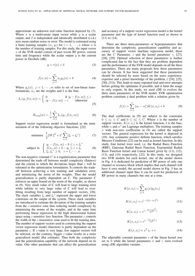
i ≤ C. Where s is the number ofsupport vectors, K(x, xi) is the kernel function, b is the bias,while α and α∗ are Lagrange multipliers. The training samplesx with non-zero coefficients in (9) are called the supportvectors. The general expression for the kernel is depicted in(10). Any symmetric positive definite function, which satisfiesMercers Conditions [22] can be used as kernel function. In thisstudy, four kernel were used, i.e. the Radial Basis Function(RBF), Gaussian Radial Basis Function, Exponential RadialBasis Function kernel and Linear kernel given by (11), (12),(13), and (14) respectively, [22]. In this study, we designedtwo SVR models for each kernel, one of the model shownin Fig. 4 is dedicated for prediction of RF power of only onechannel or resource block which implies that each channel willhave it own model; the second model shown in Fig. 5 has anadditional channel input thus it can be used for prediction ofRF power in many channels but one at a time.

K(x, xi) =

m∑

j=1

gj(x)gj(xi) (10)

K(x, xi) = e(−γ‖x−xi‖2) (11)

K(x, xi) = e(−‖x−xi‖

2

2σ2 )(12)

K(x, xi) = e(−‖x−xi‖

2σ2 )(13)

K(x, xi) = xTxi + c (14)

The adjustable constant parameter c of the linear kernel wasset to 0 while the kernel parameters σ and γ were evolvedusing cDE algorithm variants.


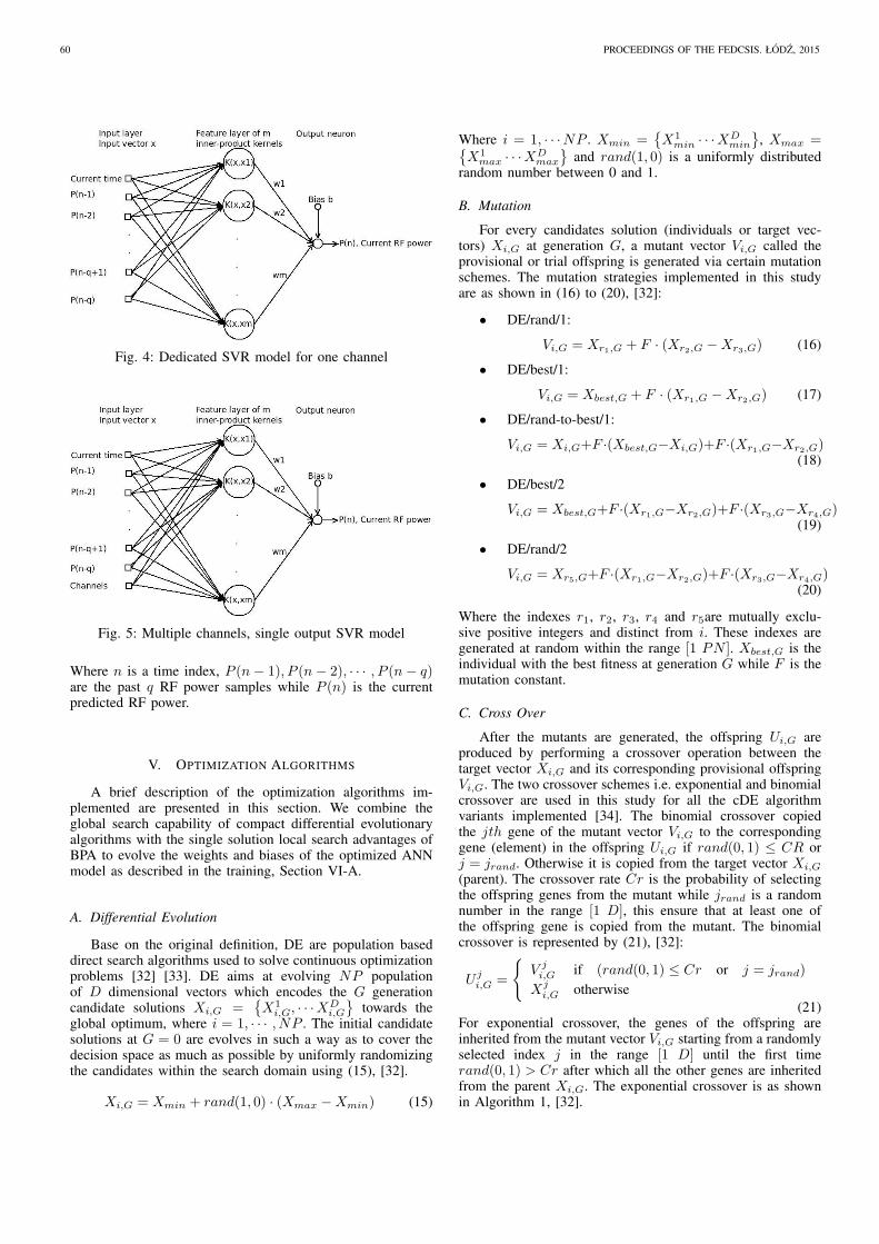
Fig. 4: Dedicated SVR model for one channel

Fig. 5: Multiple channels, single output SVR model

Where n is a time index, P (n− 1), P (n− 2), · · · , P (n− q)are the past q RF power samples while P (n) is the currentpredicted RF power.

V. OPTIMIZATION ALGORITHMS

A brief description of the optimization algorithms im-plemented are presented in this section. We combine theglobal search capability of compact differential evolutionaryalgorithms with the single solution local search advantages ofBPA to evolve the weights and biases of the optimized ANNmodel as described in the training, Section VI-A.

A. Differential Evolution

Base on the original definition, DE are population baseddirect search algorithms used to solve continuous optimizationproblems [32] [33]. DE aims at evolving NP populationof D dimensional vectors which encodes the G generationcandidate solutions Xi,G =

{

X1i,G, · · ·X

Di,G

}

towards theglobal optimum, where i = 1, · · · , NP . The initial candidatesolutions at G = 0 are evolves in such a way as to cover thedecision space as much as possible by uniformly randomizingthe candidates within the search domain using (15), [32].

Xi,G = Xmin + rand(1, 0) · (Xmax −Xmin) (15)

Where i = 1, · · ·NP . Xmin ={

X1min · · ·X

Dmin

}

, Xmax ={

X1max · · ·X

Dmax

}

and rand(1, 0) is a uniformly distributedrandom number between 0 and 1.

B. Mutation

For every candidates solution (individuals or target vec-tors) Xi,G at generation G, a mutant vector Vi,G called theprovisional or trial offspring is generated via certain mutationschemes. The mutation strategies implemented in this studyare as shown in (16) to (20), [32]:

• DE/rand/1:

Vi,G = Xr1,G + F · (Xr2,G −Xr3,G) (16)

• DE/best/1:

Vi,G = Xbest,G + F · (Xr1,G −Xr2,G) (17)

• DE/rand-to-best/1:

Vi,G = Xi,G+F ·(Xbest,G−Xi,G)+F ·(Xr1,G−Xr2,G)(18)

• DE/best/2

Vi,G = Xbest,G+F ·(Xr1,G−Xr2,G)+F ·(Xr3,G−Xr4,G)(19)

• DE/rand/2

Vi,G = Xr5,G+F ·(Xr1,G−Xr2,G)+F ·(Xr3,G−Xr4,G)(20)

Where the indexes r1, r2, r3, r4 and r5are mutually exclu-sive positive integers and distinct from i. These indexes aregenerated at random within the range [1 PN ]. Xbest,G is theindividual with the best fitness at generation G while F is themutation constant.

C. Cross Over

After the mutants are generated, the offspring Ui,G areproduced by performing a crossover operation between thetarget vector Xi,G and its corresponding provisional offspringVi,G. The two crossover schemes i.e. exponential and binomialcrossover are used in this study for all the cDE algorithmvariants implemented [34]. The binomial crossover copiedthe jth gene of the mutant vector Vi,G to the correspondinggene (element) in the offspring Ui,G if rand(0, 1) ≤ CR orj = jrand. Otherwise it is copied from the target vector Xi,G

(parent). The crossover rate Cr is the probability of selectingthe offspring genes from the mutant while jrand is a randomnumber in the range [1 D], this ensure that at least one ofthe offspring gene is copied from the mutant. The binomialcrossover is represented by (21), [32]:

Uji,G =

{

Vji,G if (rand(0, 1) ≤ Cr or j = jrand)

Xji,G otherwise

(21)For exponential crossover, the genes of the offspring areinherited from the mutant vector Vi,G starting from a randomlyselected index j in the range [1 D] until the first timerand(0, 1) > Cr after which all the other genes are inheritedfrom the parent Xi,G. The exponential crossover is as shownin Algorithm 1, [32].


Algorithm 1: Exponential Crossover

Ui,G = Xi,G

2: generate j = randi(1, D)U

ji,G = V

ji,G

4: k = 1while rand (0, 1) ≤ Cr AND k < D do

6: Uji,G = V

ji,G

j = j + 18: if j == n then

j = 110: end if

k = k + 112: end while

end

D. Selection Process

After every generation, the fitness function of each off-spring Ui,G and the corresponding parent Xi,G are computed.A greedy selection schemes is used in which if the fitnessfunction of the offspring is less than or equal to that of itparent, the offspring will replace the corresponding parent inthe next generation otherwise the parent will be maintainedamong the next generation individuals. At the end of thegeneration, the most fittest individual (global best) amongthe final evolved solutions is selected. The DE algorithmpseudocode is depicted in Algorithm 2.

Algorithm 2: Differential Evolution

Generate an initial population XG=0 of Np individuals.2: Evaluate fitness of each individuals (solutions).

while termination condition is not met (Generation) do4: for i = 1 to Np do

Evaluate parent (Xi,G) fitness .6: Generate trial offspring Vi,G by mutation using

(16).Generate offspring Ui,G by either binomialcrossover or exponential crossover.

8: Evaluate offspring (Ui,G) fitnessend for

10: for i = 1 to Np doSelection Process:

12: Form the next generation solutions by selecting thebest between parents and their offspring

end for14: end while

end

VI. COMPACT DIFFERENTIAL EVOLUTION

Compact differential evolution (cDE) algorithm is achievedby incorporating the update logic of real values compactgenetic algorithm (rcGA) within DE frame work [35] [36] [37].The steps involves in cDE is as follows: A (2 x n) probabilityvector PV consisting of the mean µ and standard deviation σis generated. where n is the dimensionality of the problem (inthis case the number of weights and biases). At initialization,µ was set to 0 while σ was set to a very large value 10,in order to simulate a uniform distribution. A solution calledthe elite is sampled from the PV. At each generation (step)other candidate solutions are sampled from the PV according

to the mutation schemes adopted as described in Section V-B,e.g. for DE/rand/1 three candidate solutions Xr1 , Xr2 andXr3 are sampled. Without lost of generality, each designedvariable Xr1 [i] belonging to a candidate solution Xr1 , isobtained from the PV as follows: For each dimension indexedby i, a truncated Gaussian probability density function (PDF)with mean µ[i] and standard deviation σ[i] is assigned. Thetruncated PDF is defined by (22). The CDF of the truncatedPDF is obtained. A random number rand(0,1) is sampled froma uniform distribution. Xr1 [i] is obtained by applying therandom number rand(0,1) generated to the inverse functionof the CDF. Since both the PDF and CDF are truncatedor normalized within the range [-1, 1]; the actual value ofXr1 [i] within the true decision space of [a, b] is obtain as

(Xr1 [i] + 1) (b−a)2 + a. The mutant (provisional offspring) is

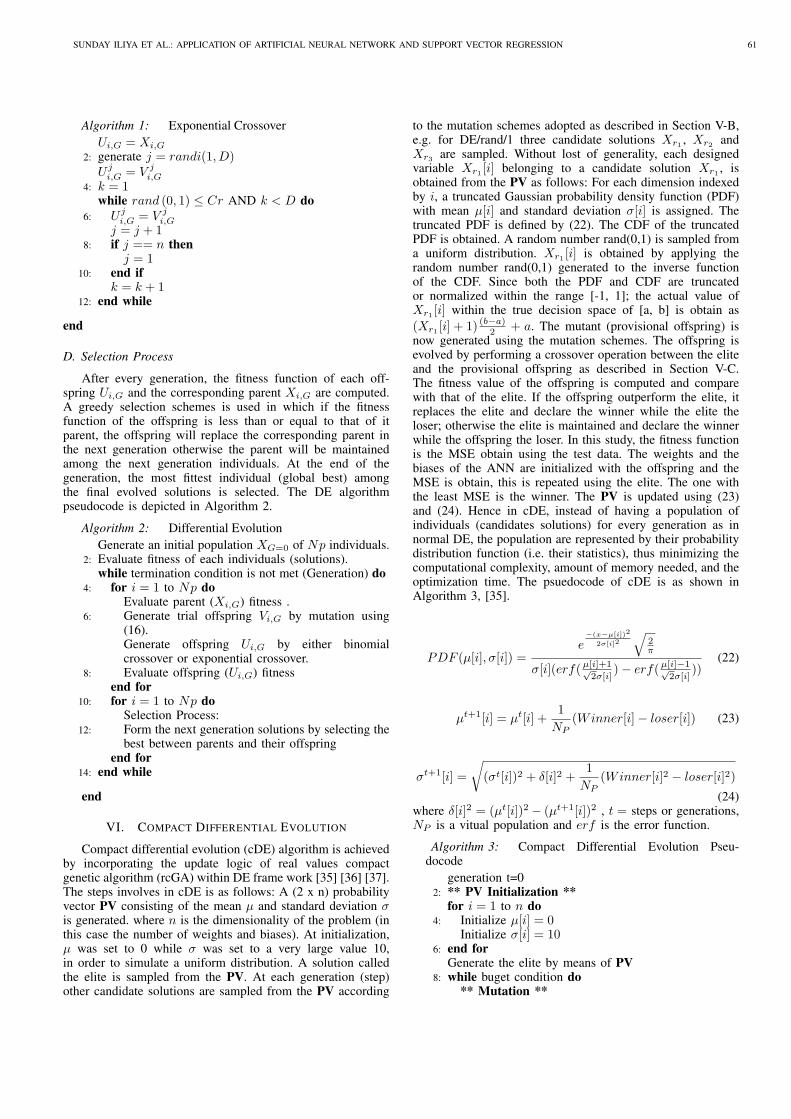
now generated using the mutation schemes. The offspring isevolved by performing a crossover operation between the eliteand the provisional offspring as described in Section V-C.The fitness value of the offspring is computed and comparewith that of the elite. If the offspring outperform the elite, itreplaces the elite and declare the winner while the elite theloser; otherwise the elite is maintained and declare the winnerwhile the offspring the loser. In this study, the fitness functionis the MSE obtain using the test data. The weights and thebiases of the ANN are initialized with the offspring and theMSE is obtain, this is repeated using the elite. The one withthe least MSE is the winner. The PV is updated using (23)and (24). Hence in cDE, instead of having a population ofindividuals (candidates solutions) for every generation as innormal DE, the population are represented by their probabilitydistribution function (i.e. their statistics), thus minimizing thecomputational complexity, amount of memory needed, and theoptimization time. The psuedocode of cDE is as shown inAlgorithm 3, [35].

PDF (µ[i], σ[i]) =e

−(x−µ[i])2

2σ[i]2

√

2π

σ[i](erf(µ[i]+1√2σ[i]

)− erf(µ[i]−1√2σ[i]

))(22)

µt+1[i] = µt[i] +1

NP

(Winner[i]− loser[i]) (23)

σt+1[i] =

√

(σt[i])2 + δ[i]2 +1

NP

(Winner[i]2 − loser[i]2)

(24)where δ[i]2 = (µt[i])2 − (µt+1[i])2 , t = steps or generations,NP is a vitual population and erf is the error function.

Algorithm 3: Compact Differential Evolution Pseu-docode

generation t=02: ** PV Initialization **

for i = 1 to n do4: Initialize µ[i] = 0

Initialize σ[i] = 106: end for

Generate the elite by means of PV8: while buget condition do

** Mutation **


10: Generate 3 or more individuals according to themutation schemes e.g. Xr1 , Xr2 and Xr3 by meansof PVCompute the mutant V = Xr1 + F · (Xr2 −Xr3)

12: ** Crossover **U = V , where U = offspring

14: for i = 1 : N doGenerate rand(0,1)

16: if rand(0, 1) > Cr thenU [i] = elite[i]

18: end ifend for

20: ** Elite Selcetion **[ Winner Loser] = compete(U, elite)

22: if U == Winner thenelite = U

24: end if** PV Update **

26: for i = 1 : n doµt+1[i] = µt[i] + 1

NP(Winner[i]− loser[i])

28: σt+1[i] =√

(σt[i])2 + δ[i]2 + γ[i]2

Where: δ[i]2 = (µt[i])2 − (µt+1[i])2

30: γ[i]2 = 1NP

(Winner[i]2 − loser[i]2)end for

32: t = t+ 1end while

end

A. Training of ANN and SVM

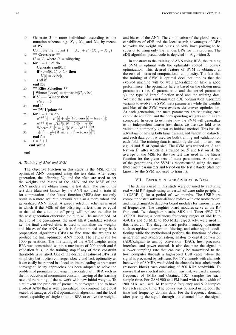
The objective function in this study is the MSE of theoptimized ANN computed using the test data. After everygeneration, the offspring UG and the elite are used to setthe weights and biases of the ANN and the MSE of theANN models are obtain using the test data. The use of thetest data (data not known by the ANN nor used to train it)for computation of the fitness function (MSE) does not onlyresult in a more accurate network but also a more robust andgeneralized ANN model. A greedy selection schemes is usedin which if the MSE of the offspring is less than or equalto that of the elite, the offspring will replace the elite inthe next generation otherwise the elite will be maintained. Atthe end of the generations, the most fittest candidate solutioni.e. the final evolved elite; is used to initialize the weightsand biases of the ANN which is further trained using backpropagation algorithms (BPA) to fine tune the weights toproduce the final optimized ANN model. The cDE is run for1000 generations. The fine tuning of the ANN weights usingBPA was constrained within a maximum of 200 epoch and 6validation fails, i.e the training stop if any of these constrainthresholds is satisfied. One of the desirable feature of BPA is itsimplicity but it often converges slowly and lack optimality asit can easily be trapped in a local optimum leading to prematureconvergent. Many approaches has been adopted to solve theproblem of premature convergent associated with BPA such asthe introduction of momentum constant, varying of the learningrate and retraining of the network with new initial weights. Tocircumvent the problem of premature convergent, and to havea robust ANN that is well generalized, we combine the globalsearch advantages of cDE optimization algorithm and the localsearch capability of single solution BPA to evolve the weights

and biases of the ANN. The combination of the global searchcapabilities of cDE and the local search advantages of BPAto evolve the weight and biases of ANN have proving to besuperior to using only the famous BPA for this problem. ThecDE algorithm pseudocode is depicted in Algorithm 3.

In constract to the training of ANN using BPA, the trainingof SVM is optimal with the optimality rooted in convexoptimization. This desired feature of SVM is obtained atthe cost of increased computational complexity. The fact thatthe training of SVM is optimal does not implies that theevolved machine will be well generalized or have a goodperformance. The optimality here is based on the chosen metaparameters ( i.e. C parameter, ε and the kernel parameterγ), the type of kernel function used and the training data.We used the same randomization cDE optimization algorithmvariants to evolve the SVM meta parameters while the weightsand bias of the SVM were evolves via convex optimization.At each generation, the meta parameters are set using eachcandidate solution, and the corresponding weights and bias arecomputed. In order to estimate how the SVM will generalizeto an independent dataset (test data), we use two fold crossvalidation commonly known as holdout method. This has theadvantage of having both large training and validation datasets,and each data point is used for both training and validation oneach fold. The training data is randomly divided into two setse.g. A and B of equal size. The SVM was trained on A andtest on B, after which it is trained on B and test on A, theaverage of the MSE for the two test was used as the fitnessfunction for the given sets of meta parameters. At the endof the generations, the SVM is reconstructed using the mostfittest meta parameters and tested on the test datasets (data notknown by the SVM nor used to train it).

VII. EXPERIMENT AND SIMULATION DATA

The datasets used in this study were obtained by capturingreal world RF signals using universal software radio peripheral1 (USRP 1) for a period of two months. The USRP arecomputer hosted software-defined radios with one motherboardand interchangeable daughter board modules for various rangesof frequencies. The daughter board modules serve as the RFfront end. Two daughter boards, SBX and Tuner 4937 DI53X7901, having a continuous frequency ranges of 4MHz to4.4GHz and 50 MHz to 860 MHz respectively, were used inthis research. The daughterboard perform analog operationssuch as up/down-conversion, filtering, and other signal condi-tioning while the motherboard perform the functions of clockgeneration and synchronization, analog to digital conversion(ADC),digital to analog conversion (DAC), host processorinterface, and power control. It also decimate the signal toa lower sampling rate that can easily be transmitted to thehost computer through a high-speed USB cable where thesignal is processed by software. For TV channels with channelsbandwidth of 8 MHz, we divided the channels into subchannels(resource block) each consisting of 500 KHz bandwidth. Toensure that no spectral information was lost, we used a samplefrequency of 1MHz and obtained 1024 samples for eachsample time. For GSM 900 and FM band with a bandwidth of200 KHz, we used 1MHz sample frequency and 512 samplesfor each sample time. The power was obtained using both thetime and frequency domain data. For the frequency domain,after passing the signal through the channel filter, the signal


was windowed using a hamming window in order to reducespectral leakage. The stream of the data was converted toa vector and decimated to a lower sampling rate that caneasily be processed by the host computer at run time using theinbuilt decimation block in gnu-radio. This is then convertedto the frequency domain and the magnitudes of the bins werepassed to a probe sink. The choice of probe sink is essentialbecause it can only hold the current data and does not increasethereby preventing stack overflow or a segmentation fault. Thisallows Python to grab the data at run time for further analysis.The interval of time between consecutive sample data wasselected at a random value between 5 seconds and 30 seconds.The choice of this range is based on the assumption that forany TV programme, FM broadcast or GSM calls, will lastfor not less than 5 to 30 seconds. In order to capture allpossible trends, the time between consecutive sample data isselected at random within the given range instead of usingregular intervals. For the VHF and FM band we captured RFsignals from 54MHz to 110MHz and 470 to 670MHz for theVHF TV bands. For the GSM band, 62 down-link channels(935MHz to 953.3MHz) and 62 uplink channels (890MHzto 908.3MHz) were captured. The real world RF data wasdivided into three subsets, randomly selected with 60% usedfor training the ANN, 20% for validation and 20% for testingthe trained ANN model. The training or estimation data werethe only known data sources used in training the ANN. Thetest data set was unknown to the network i.e. they are not usedin training the network rather are used in testing the trainedANN as a measure of the generalization performance of theANN model. The ANN design, optimization and the simulationwere done in Matlab while the capturing of the data and thesignal processing were implemented using gnu-radio which isa combination of Python and C++.

VIII. DELAYED INPUTS SENSITIVITY ANALYSIS

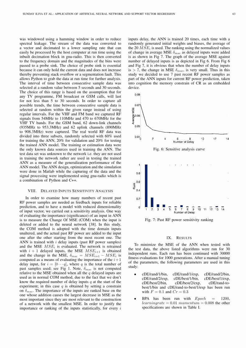
In order to examine how many numbers of recent pastRF power samples are needed as feedback inputs for reliableprediction, and to have a model with reduced dimensionalityof input vector, we carried out a sensitivity analysis. One wayof evaluating the importance (significance) of an input in ANNis to measure the Change Of MSE (COM) when the input isdeleted or added to the neural network [38]. In this study,the COM method is adopted with the time domain inputsunaltered, and the actual past RF power are added to the inputone after the other starting from the most recent one. TheANN is trained with i delay inputs (past RF power samples)and the MSE MSEi is evaluated. The network is retrainedwith i + 1 delayed inputs, the MSE MSEi+1 is obtainedand the change in the MSE, δmse = MSEi+1 − MSEi iscomputed as a means of evaluating the importance of the i+1delay input, for i = [0 · · · q], where q is the total number ofpast samples used; see Fig 1. Note, δmse is not computedrelative to the MSE obtained when all the q delayed inputs areused as in normal COM method, due to the fact that we don’tknow the required number of delay inputs q at the start of theexperiment; in this case q is obtained by setting a constrainon δmse. The importance of the inputs are ranked base on theone whose addition causes the largest decrease in MSE as themost important since they are most relevant to the constructionof a network with the smallest MSE. In order to justify theimportance or ranking of the inputs statistically, for every i

inputs delay, the ANN is trained 20 times, each time with arandomly generated initial weights and biases, the average ofthe 20 MSEi is used. The ranking using the normalized valuesof change in average MSE δmse as delayed inputs were addedis as shown in Fig 7. The graph of the average MSE againstnumber of delayed inputs is as depicted in Fig 6. From Fig 6and Fig 7, it is obvious that when the number of delay inputsis > 7, the change in MSE δmse, is very small. Thus in thisstudy we decided to use 7 past recent RF power samples aspart of the ANN inputs for current RF power prediction, takeninto cognition the memory constrain of CR as an embeddeddevice.

Fig. 6: Sensitive analysis curve

Fig. 7: Past RF power sensitivity ranking

IX. RESULTS

To minimize the MSE of the ANN when tested withthe test data, the above listed algorithms were run for 30independent runs. Each run has been continued with 30000fitness evaluations for 1000 generations. After a manual tuningof the parameters, the following parameters are used in thisstudy:

• cDE/rand/1/bin, cDE/rand/1/exp, cDE/rand/2/bin,cDE/rand/2/exp, cDE/best/1/bin, cDE/best/1/exp,cDE/best/2/bin, cDE/best/2/exp, cDE/rand-to-best/1/bin and cDE/rand-to-best/1/exp has been runwith F = 0.1 and Cr = 0.3

• BPA has been run with Epoch = 1200,learningrate = 0.01 mumentum = 0.008 the otherspecifications are shown in Table I.


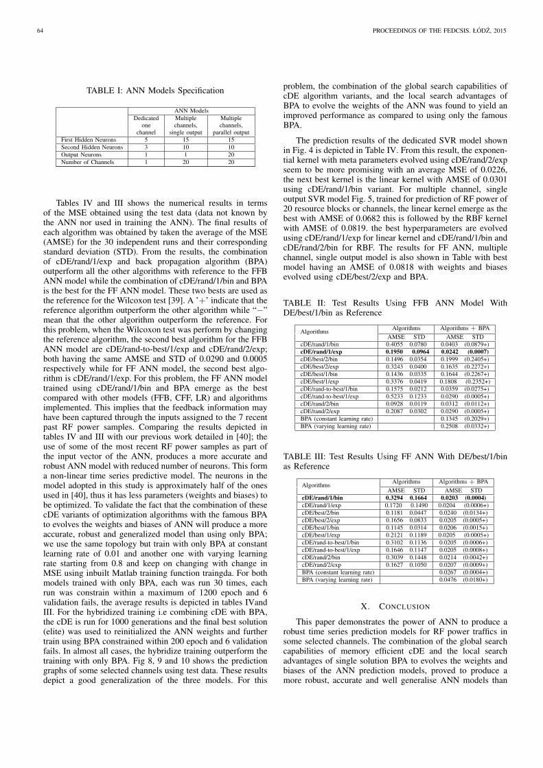
TABLE I: ANN Models Specification

ANN Models

Dedicated Multiple Multiple

one channels, channels,

channel single output parallel output

First Hidden Neurons 5 15 15

Second Hidden Neurons 3 10 10

Output Neurons 1 1 20

Number of Channels 1 20 20

Tables IV and III shows the numerical results in termsof the MSE obtained using the test data (data not known bythe ANN nor used in training the ANN). The final results ofeach algorithm was obtained by taken the average of the MSE(AMSE) for the 30 independent runs and their correspondingstandard deviation (STD). From the results, the combinationof cDE/rand/1/exp and back propagation algorithm (BPA)outperform all the other algorithms with reference to the FFBANN model while the combination of cDE/rand/1/bin and BPAis the best for the FF ANN model. These two bests are used asthe reference for the Wilcoxon test [39]. A ’+’ indicate that thereference algorithm outperform the other algorithm while “−”mean that the other algorithm outperform the reference. Forthis problem, when the Wilcoxon test was perform by changingthe reference algorithm, the second best algorithm for the FFBANN model are cDE/rand-to-best/1/exp and cDE/rand/2/exp;both having the same AMSE and STD of 0.0290 and 0.0005respectively while for FF ANN model, the second best algo-rithm is cDE/rand/1/exp. For this problem, the FF ANN modeltrained using cDE/rand/1/bin and BPA emerge as the bestcompared with other models (FFB, CFF, LR) and algorithmsimplemented. This implies that the feedback information mayhave been captured through the inputs assigned to the 7 recentpast RF power samples. Comparing the results depicted intables IV and III with our previous work detailed in [40]; theuse of some of the most recent RF power samples as part ofthe input vector of the ANN, produces a more accurate androbust ANN model with reduced number of neurons. This forma non-linear time series predictive model. The neurons in themodel adopted in this study is approximately half of the onesused in [40], thus it has less parameters (weights and biases) tobe optimized. To validate the fact that the combination of thesecDE variants of optimization algorithms with the famous BPAto evolves the weights and biases of ANN will produce a moreaccurate, robust and generalized model than using only BPA;we use the same topology but train with only BPA at constantlearning rate of 0.01 and another one with varying learningrate starting from 0.8 and keep on changing with change inMSE using inbuilt Matlab training function traingda. For bothmodels trained with only BPA, each was run 30 times, eachrun was constrain within a maximum of 1200 epoch and 6validation fails, the average results is depicted in tables IVandIII. For the hybridized training i.e combining cDE with BPA,the cDE is run for 1000 generations and the final best solution(elite) was used to reinitialized the ANN weights and furthertrain using BPA constrained within 200 epoch and 6 validationfails. In almost all cases, the hybridize training outperform thetraining with only BPA. Fig 8, 9 and 10 shows the predictiongraphs of some selected channels using test data. These resultsdepict a good generalization of the three models. For this

problem, the combination of the global search capabilities ofcDE algorithm variants, and the local search advantages ofBPA to evolve the weights of the ANN was found to yield animproved performance as compared to using only the famousBPA.

The prediction results of the dedicated SVR model shownin Fig. 4 is depicted in Table IV. From this result, the exponen-tial kernel with meta parameters evolved using cDE/rand/2/expseem to be more promising with an average MSE of 0.0226,the next best kernel is the linear kernel with AMSE of 0.0301using cDE/rand/1/bin variant. For multiple channel, singleoutput SVR model Fig. 5, trained for prediction of RF power of20 resource blocks or channels, the linear kernel emerge as thebest with AMSE of 0.0682 this is followed by the RBF kernelwith AMSE of 0.0819. the best hyperparameters are evolvedusing cDE/rand/1/exp for linear kernel and cDE/rand/1/bin andcDE/rand/2/bin for RBF. The results for FF ANN, multiplechannel, single output model is also shown in Table with bestmodel having an AMSE of 0.0818 with weights and biasesevolved using cDE/best/2/exp and BPA.

TABLE II: Test Results Using FFB ANN Model WithDE/best/1/bin as Reference

AlgorithmsAlgorithms Algorithms + BPA

AMSE STD AMSE STD

cDE/rand/1/bin 0.4055 0.0780 0.0403 (0.0879+)

cDE/rand/1/exp 0.1950 0.0964 0.0242 (0.0007)

cDE/best/2/bin 0.1496 0.0354 0.1999 (0.2405+)

cDE/best/2/exp 0.3243 0.0400 0.1635 (0.2272+)

cDE/best/1/bin 0.1436 0.0335 0.1644 (0.2267+)

cDE/best/1/exp 0.3376 0.0419 0.1808 (0.2352+)

cDE/rand-to-best/1/bin 0.1575 0.0212 0.0359 (0.0275+)

cDE/rand-to-best/1/exp 0.5233 0.1233 0.0290 (0.0005+)

cDE/rand/2/bin 0.0928 0.0119 0.0312 (0.0112+)

cDE/rand/2/exp 0.2087 0.0302 0.0290 (0.0005+)

BPA (constant learning rate) 0.1345 (0.2029+)

BPA (varying learning rate) 0.2508 (0.0332+)

TABLE III: Test Results Using FF ANN With DE/best/1/binas Reference

AlgorithmsAlgorithms Algorithms + BPA

AMSE STD AMSE STD

cDE/rand/1/bin 0.3294 0.1664 0.0203 (0.0004)

cDE/rand/1/exp 0.1720 0.1490 0.0204 (0.0006+)

cDE/best/2/bin 0.1181 0.0447 0.0240 (0.0134+)

cDE/best/2/exp 0.1656 0.0833 0.0205 (0.0005+)

cDE/best/1/bin 0.1145 0.0314 0.0206 (0.0015+)

cDE/best/1/exp 0.2121 0.1189 0.0205 (0.0005+)

cDE/rand-to-best/1/bin 0.3102 0.1136 0.0205 (0.0006+)

cDE/rand-to-best/1/exp 0.1646 0.1147 0.0205 (0.0008+)

cDE/rand/2/bin 0.3039 0.1448 0.0214 (0.0042+)

cDE/rand/2/exp 0.1627 0.1050 0.0207 (0.0009+)

BPA (constant learning rate) 0.0267 (0.0004+)

BPA (varying learning rate) 0.0476 (0.0180+)

X. CONCLUSION

This paper demonstrates the power of ANN to produce arobust time series prediction models for RF power traffics insome selected channels. The combination of the global searchcapabilities of memory efficient cDE and the local searchadvantages of single solution BPA to evolves the weights andbiases of the ANN prediction models, proved to produce amore robust, accurate and well generalise ANN models than


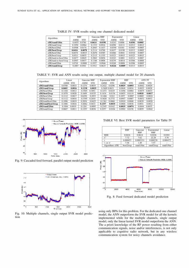
TABLE IV: SVR results using one channel dedicated model

AlgorithmsRBF Gaussian RBF Exponential Linear

AMSE STD AMSE STD AMSE STD AMSE STD

cDE/rand/1/bin 0.4055 0.0780 0.0614 0.0198 0.0243 0.0006 0.0301 0.0005

cDE/rand/1/exp 0.1950 0.0964 0.1333 0.0916 0.0298 0.0111 0.0313 0.0012

cDE/best/2/bin 0.0508 0.0174 0.2043 0.1437 0.0350 0.0181 0.0303 0.0003

cDE/best/2/exp 0.0416 0.0078 0.2114 0.0788 0.0437 0.0190 0.0313 0.0005

cDE/best/1/bin 0.0474 0.0015 0.2670 0.0385 0.0266 0.0041 0.0310 0.0007

cDE/best/1/exp 0.0511 0.0035 0.2115 0.1355 0.0323 0.0015 0.0323 0.0015

cDE/rand-to-best/1/bin 0.0477 0.0045 0.2062 0.0856 0.0243 0.0001 0.0314 0.0007

cDE/rand-to-best/1/exp 0.0507 0.0037 0.1346 0.0806 0.0239 0.0014 0.0306 0.0008

cDE/rand/2/bin 1.6718 0.0000 0.1937 0.0946 0.0248 0.0008 0.0306 0.0005

cDE/rand/2/exp 0.2087 0.0302 0.1912 0.0625 0.0226 0.0009 0.0313 0.0015

TABLE V: SVR and ANN results using one output, multiple channel model for 20 channels

AlgorithmsLinear Gaussian RBF Exponential RBF RBF ANN FF

AMSE STD AMSE STD AMSE STD AMSE STD AMSE STD

cDE/rand/1/bin 0.0700 0.0033 0.1274 0.0035 0.2422 0.0296 0.0819 0.0093 0.0842 0.0029

cDE/rand/1/exp 0.0682 0.0016 0.1238 0.0025 0.2609 0.0651 0.0848 0.0016 0.0835 0.0028

cDE/best/2/bin 0.1104 0.0012 0.3565 0.3051 0.1472 0.0225 0.1056 0.0084 0.0875 0.0033

cDE/best/2/exp 0.1078 0.0020 0.1609 0.0155 0.1434 0.0136 0.0855 0.0119 0.0818 0.0017

cDE/best/1/bin 0.1112 0.0017 0.6258 0.4953 0.1466 0.012 0.1057 0.0087 0.0869 0.0018

cDE/best/1/exp 0.1112 0.0016 0.3395 0.2010 0.3020 0.2732 0.0947 0.0087 0.0832 0.0032

cDE/rand/best/1/bin 0.1096 0.0019 0.2854 0.0425 0.1361 0.0060 0.0910 0.0040 0.0839 0.0028

cDE/rand/best/1/exp 0.1086 0.0016 0.4062 0.0433 0.1357 0.0035 0.0868 0.0036 0.0851 0.0012

cDE/rand/2/bin 0.1094 0.0019 0.1281 0.0095 0.2345 0.0162 0.0819 0.0074 0.0844 0.0035

cDE/rand/2/exp 0.0687 0.0011 0.1255 0.0036 0.2257 0.0104 0.0902 0.0156 0.0859 0.0042

Fig. 9: Cascaded feed forward, parallel output model prediction

Fig. 10: Multiple channels, single output SVR model predic-tion

TABLE VI: Best SVR model parameters for Table IV

Kernel

RBF Gaussian Exponential Linear

RBF RBF

MSE 0.0416 0.0614 0.0226 0.0301

C 7.72 7.62 22.28 3.76

ε 0.000653 0.0003331 0.000228 0.000472

γ or σ 7.38 1.49 7.57 -

Algorithms cDE/ best/2/exp rand/1/bin rand/2/exp rand/1/bin

Fig. 8: Feed forward dedicated model prediction

using only BPA for this problem. For the dedicated one channelmodel, the ANN outperform the SVR model for all the kernelsimplemented while for the multiple channels, single outputmodel, only the linear kernel SVR model outperform the ANN.The a priori knowledge of the RF power resulting from eithercommunication signals, noise and/or interferences, is not onlyapplicable to cognitive radio network, but in any wirelesscommunication system for noisy channels avoidance.


ACKNOWLEDGMENT

This work is supported by Petroleum Technology Devel-opment Fun (PTDF) Scholarship, Nigeria and De MontfortUniversity, United Kingdom.

REFERENCES

[1] FCC, “Federal comminucation commission notice of inquiry and noticeof proposed rule making, in the matter of establishment of an inter-ference temperature metric to quantify and manage interference andto expand available unlicensed operation in certain fixed, mobile andsatellite frequency bands,” no. 03-237, November 13, 2003.

[2] V. Valenta, R. Marsalek, G. Baudoin, M. Villegas, M. Suarez, andF. Robert, “Survey on spectrum utilization in europe: Measurements,analyses and observations,” in Cognitive Radio Oriented Wireless Net-

works Communications (CROWNCOM), 2010 Proceedings of the Fifth

International Conference on, June 2010, pp. 1–5.

[3] S. Haykin, D. J. Thomson, and J. H. Reed, “Spectrum sensing forcognitive radio,” in IEEE Transactions on Cognitive Radio, May 2009.

[4] J. Oh and W. Choi, “A hybrid cognitive radio system: A combination ofunderlay and overlay approaches,” in IEEE Transactions on Cognitive

Radio, 2009.

[5] C. Stevenson, G. Chouinard, Z. Lei, W. Hu, J. Stephen, and W. Cald-well, “The first cognitive radio wireless regional area network standard,”in IEEE 802.22, 2009.

[6] X. Xing, T. Jing, W. Cheng, Y. Huo, and X. Cheng, “Spectrumprediction in cognitive radio networks,” in 1536-1284/13/$25.00 c©2013

IEEE Transactions on Wireless Communications, April 2013.

[7] A. M. Wyglinski, M. Nekovee, and Y. T. Hou, Cognitive Radio

Communications and Networks, 2009.

[8] M. Subhedar and G. Birajdar, “Spectrum sensing techniques in cognitiveradio networks: A survey,” International Journal of Next-Generation

Networks, vol. 3, no. 2, pp. 37–51, 2011.

[9] T. W. Rondeau, B. Le, C. J. Rieser, and C. W. Bostian, “Cognitiveradios with genetic algorithms: Intelligent control of software definedradios,” in c©2004 SDR Forum, Proceeding of the SDR 2004 Technical

Conference and Product Exposition, 2004.

[10] S. K. Udgata, K. P. Kumar, and S. L. Sabat, “Swarm intelligence basedresource allocation algorithm for cognitive radio network,” in Paral-

lel Distributed and Grid Computing (PDGC), 2010 1st International

Conference on, Oct 2010, pp. 324–329.

[11] M. Matinmikko, J. Del Ser, T. Rauma, and M. Mustonen, “Fuzzy-logicbased framework for spectrum availability assessment in cognitive radiosystems,” Selected Areas in Communications, IEEE Journal on, vol. 31,no. 11, pp. 2173–2184, November 2013.

[12] L. Giupponi and A. Perez, “Fuzzy-based spectrum handoff in cognitiveradio networks,” 2008.

[13] Y. Chen and H.-S. Oh, “A survey of measurement-based spectrumoccupancy modelling for cognitive radios,” in 1553-877X c©2013 IEEE

IEEE Communications Surveys and Tutorials, 2013.

[14] R. Azmi, “Support vector machine based white space predictors forcognitive radio,” Master’s thesis, 2011.

[15] O. Winston, A. Thomas, and W. OkelloOdongo, “Optimizing neuralnetwork for tv idle channel prediction in cognitive radio using particleswarm optimization,” in Computational Intelligence, Communication

Systems and Networks (CICSyN), 2013 Fifth International Conference

on, June 2013, pp. 25–29.

[16] M. I. Taj and M. Akil, “Cognitive radio spectrum evolution predictionusing artificial neural networks based mutivariate time series mod-elling,” in European Wireless, Vienna Austria, April 2011.

[17] X. Li and S. A. Zekavat, “Traffic pattern prediction and performanceinvestigation for cognitive radio systems,” in IEEE Communication

Society, WCNC Proceedings, 2008.

[18] S. Hiremath and S. K. Patra, “Transmission rate prediction for cognitiveradio using adaptive neural fuzzy inference system,” in IEEE 5th

International Conference on Industrial and Information Systems (ICIIS),

India, Aug 2010.

[19] S. Geirhofer, J. Z. Sun, L. Tong, and B. M. Sadler, “Cognitive frequencyhopping based on interference prediction: Theory and experimentalresults,” vol. 13, no. 2, march 17, 2009.

[20] Z. Tabakovic, S. Grgic, and M. Grgic, “Fuzzy logic power control incognitive radio,” in IEEE transactions, 2009.

[21] Z. Lin, X. Jian, L. Huang, and Y. Yao, “Energy prediction basedspectrum sensing approach for cognitive radio network,” in 978-1-4244-

3693-4/09/$25.00 c©2009 IEEE, 2009.

[22] S. Haykin, Neural Networks and Learning Machines, 3rd ed., 2008.

[23] Z. Jianli, “Based on neural network spectrum prediction of cognitiveradio,” in 978-1-4577-0321-8/11/$26.00 c©2011 IEEE, 2011.

[24] V. Vapnik, The nature of statistical learning theory. Springer-VerlagNew York Inc, 1999.

[25] V. Vapnik, Statistical learning theory. New York: Wiley, 1998.

[26] E. Alpaydin, Introduction to Machine Learning, ser. Adaptive compu-tation and machine learning. MIT Press, 2004.

[27] V. Kecman, Learning and soft computing. MIT Press Cambridge,Mass, 2001.

[28] C. Vladimir and Y. MA, “Selection of meta-parameters for supportvector regression,” pp. 687–693, August 2002.

[29] W. Wenjian, Z. Xu, W. Lu, and X. Zhang, “Determination of the spreadparameter in the gaussian kernel for classification and regression,”vol. 55, no. 3, pp. 643–663, October 2003.

[30] V. S. Cherkassky and F. Mulier, Learning from Data: Concepts, Theory,

and Methods, 1st ed. New York, NY, USA: John Wiley and Sons, Inc.,1998.

[31] B. Scholkopf and A. J. Smola, Learning with Kernels: Support Vector

Machines, Regularization, Optimization, and Beyond. Cambridge, MA,USA: MIT Press, 2001.

[32] K. V. Price, R. Storn, and J. Lampinen, Differential Evolution: A

Practical Approach to Global Optimization. Springer, 2005.

[33] A. K. Qin, V. L. Huang, and P. N. Suganthan, “Differential evolutionalgorithm with strategy adaptation for global numerical optimization,”in IEEE Transactions on Evolutionary Computation, vol. 13, no. 2,April 2009.

[34] D. Zaharie, “A comparative analysis of crossover variants in differentialevolution,” in Proceedings of the International Multiconference on

Computer Science and Information Technology, 2007, pp. 171–181.

[35] E. Mininno, F. Neri, F. Cupertino, and D. Naso, “Compact differentialevolution,” Evolutionary Computation, IEEE Transactions on, vol. 15,no. 1, pp. 32–54, Feb 2011.

[36] G. Harik, F. Lobo, and D. Goldberg, “The compact genetic algorithm,”Evolutionary Computation, IEEE Transactions on, vol. 3, no. 4, pp.287–297, Nov 1999.

[37] C. W. Ahn and R. Ramakrishna, “Elitism-based compact geneticalgorithms,” Evolutionary Computation, IEEE Transactions on, vol. 7,no. 4, pp. 367–385, Aug 2003.

[38] A. H. Sung, “Ranking importance of input parameters of neural net-works,” Expert Systems with Applications, vol. 15, no. 3, pp. 405–411,November 1998.

[39] F. Wilcoxon, “Individual comparisons by ranking methods,” Biometrics

Bulletin, vol. 1, no. 6, pp. 80–83, 1945.

[40] S. Iliya, E. Goodyer, J. Shell, J. Gow, and M. Gongora, “Optimizedneural network using differential evolutionary and swarm intelligenceoptimization algorithms for rf power prediction in cognitive radio net-work: A comparative study,” in 978-1-4799-4998-4/14/$31.00 c©2014

IEEE International Conference on Adaptive Science and Information

Technology, 2014.


Documents

Application of Artificial Neural Network and Support Vector … · Support Vector Regression in Cognitive Radio Networks for RF Power Prediction Using Compact Differential Evolution