International Journal on Marine Navigation and Safety of Sea Transportation

Volume 6 Number 1

March 2012

57

1 INTRODUCTION

For a long time ship manoeuvring characteristics were considered to be of marginal importance. Nev-ertheless, from the operational point of view of in-land vessels, manoeuvring characteristics play a crucial role. Operating in restricted waterways sub-stantially increases the risk of accidents and disasters as a result of manoeuvring errors. To increase level of safety on the waterways, it is important to ensure that vessels have appropriate manoeuvring charac-teristics. For this purpose it is necessary to develop research methods for determining the manoeuvring properties of inland ships.

Currently, one of the more commonly used re-search methods in ship hydrodynamics are numeri-cal methods. With improvements in computing pow-er and increasingly more accurate CFD methods it is possible to simulate more complicated cases. This paper presents a numerical method for prediction of ship manoeuvrability. It is based on a mathematical model of the ship equations of motion, described in section 3. This model requires knowledge of the co-efficients of the hydrodynamic forces acting on the ship. In section 4 there is presented a method for de-termining the hydrodynamic coefficients using CFD.

On inland waters the most restrictive rules are described in Rhine Regulations. The severity of the Rhine Regulations is the result of difficult conditions

on the Rhine: a strong current and high traffic inten-sity. Vessels that fulfil these requirements are al-lowed to operate on other waterways in Europe. These regulations specify requirements for: a mini-mum speed of the vessel, the ability to stop, the abil-ity to move backwards and turning manoeuvrability. In addition, there is specified an additional manoeu-vre - "evasive action" , which is analogous to zig-zag test and is a specific requirement for inland wa-ters. The main characteristic of this evasive action [1] is the moment of switching the rudder to the op-posite side, which occurs when the ship reaches the desired angular velocity.

2 MATHEMATICAL MODEL OF SHIP MOTION

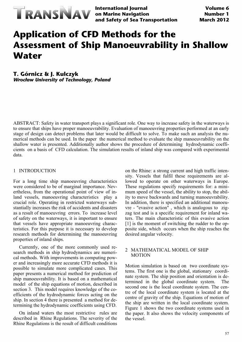
Motion simulation is based on two coordinate sys-tems. The first one is the global, stationary coordi-nate system. The ship position and orientation is de-termined in the global coordinate system. The second one is the local coordinate system. The cen-tre of the local coordinate system is located at the centre of gravity of the ship. Equations of motion of the ship are written in the local coordinate system. Figure 1 shows the two coordinate systems used in the paper. It also shows the velocity components of the vessel.

Application of CFD Methods for the Assessment of Ship Manoeuvrability in Shallow Water

T. Górnicz & J. Kulczyk Wrocław University of Technology, Poland

ABSTRACT: Safety in water transport plays a significant role. One way to increase safety in the waterways is to ensure that ships have proper manoeuvrability. Evaluation of manoeuvring properties performed at an early stage of design can detect problems that later would be difficult to solve. To make such an analysis the nu-merical methods can be used. In the paper the numerical method to evaluate the ship manoeuvrability on the shallow water is presented. Additionally author shows the procedure of determining hydrodynamic coeffi-cients on a basis of CFD calculation. The simulation results of inland ship was compared with experimental data.

58

Figure 1. Coordinate systems and velocity components of the vessel.

The movement of the ship is considered to be

planar motion (limited to three degrees of freedom). This study only analysed small velocities at

which sinkage and trimming of the ship is minimal. Therefore, these phenomena are not considered in the research..

Interaction between the hull, rudder and propel-lers are only simulated by appropriate coefficients.

In inland vessels the centre of gravity is far lower than in marine ships. In addition, the centre of gravi-ty is located near the centre of buoyancy. As a result of this , the roll of the vessel is relatively small and could also be neglected.

Wavelength on inland waterways is relatively small in proportion to the length of the vessel. In the study the influence of waves on the trajectory of the ship was not taken into consideration.

The equations of motion (1) were written for the centre of gravity of the ship. The left side of equa-tions describes the ship as a rigid body. On the right side of equations there are hydrodynamic external forces (X, Y) and the hydrodynamic moment (N) acting on the vessel.

zz

mu mvr Xmv mur YI r N

− =+ ==

(1)

where: m – vessel mass; u –longitudinal velocity; v – transversal velocity; r – yaw rate; ˙- dot, the deriva-tive of a variable over time; Izz – moment of inertia of the vessel; X,Y,N – hydrodynamic force and mo-ment acting on the vessel according to the axes of local coordinate system. Detailed information about model can be found in [2].

External hydrodynamic forces and the hydrody-namic moment acting on the ship were written like in the MMG model [3], as a sum of the compo-nents.

H P R

H R

H P R

X X X XY Y YN N N N

= + += += + +

(2)

where: XH, YH, NH – hydrodynamic forces and moment act-ing on the bare hull; XP, NP- force and moment in-duced by the operation of propellers, XR, YR, NR –forces and moment induced by flow around the rud-der.

2.1 Hull To determine the hydrodynamic forces induced by flow around the hull the following mathematical model was used [3]:

2

2 4

3 2

2 3

3 2

2 3

( ) ( )

( )

H x T vv vr y

rr vvvv

H y v r x vvv vvr

vrr rrr

H zz v r vvv vvr

vrr rrr

X m u R u X v X m vr

X r X vY m v Y v Y m u r Y v Y v r

Y vr Y rN j r N v N r N v N v r

N vr N r

− − + + + +

+ +

= − + + − + + +

+ +

= − + + + + +

+ +

=

(3)

where: mx, my – added mass coefficients, in x and y direc-tion; jzz – added inertia coefficient; RT(u) – hull re-sistance; Xvv, Xvr,..., Yv, Yr,... - coefficient of hydro-dynamic forces acting on the hull; Nv, Nr, ... – coefficients of hydrodynamic moment acting on the hull.

2.2 Rudders Hydrodynamic forces induced by rudder laying can be calculated on the basis of equations (4). The model was taken from[4].

(1 ) sin(1 ) cos( ) cos

R R N

R H N

R R H H N

X t FY a FN x a x F

δδ

δ

= − −= − += − +

(4)

where: tR - coefficient of additional drag; aH - ratio of addi-tional lateral force; xR – x-coordinate of application point of FN; xH - x-coordinate of application point of additional lateral force; δ rudder angle; FN – normal hydrodynamic force acting on the rudder.

The value of normal force FN was determined on the basis of model (5).

59

( )( )

( )

2

22

2

00

0,5·

1 (1 · ( ))2 (2 )·

( )1

10.61

cos1 (1 )·

·2 ·

N R N R

R R

R

P

R

P

PR R

P

R R

R R

F A C U

U w C g sK s s

g s Ks

Dh

wKw

s w Un P

ww ww

x r

ρ

η

η

β

α δ γ ββ β

=

= − +

− −=

−

=

−=

−

= − −

=

′= −′ ′ ′= −

(5)

where: ρ – water density; AR – rudder area; CN – normal force coefficient; UR - effective rudder inflow ve-locity; C – coefficient, dependent on ruder angle sense (C≈1.0); D – propeller diameter; hR – height of rudder; wP - wake fraction at propeller location; wR - wake fraction at rudder location; wR0 - effective wake fraction at rudder location, in straight ahead ship motion; U – total velocity of vessel; β – drift angle; n – rotational speed of propeller; P – propeller pitch; x’R – non-dimensional x-coordinate of appli-cation point of FN; r’ – non-dimensional yaw rate.

2.3 Propellers This paper uses a mathematical model of hydrody-namic forces generated by two propellers.

1 2

1 2

(1 )( )(1 )( )

P

P

X t T TN t T T d

= − += − −

(6)

where: t - thrust deduction factor; T1,T2 – thrust generated by propellers; d- distance from the axis of propeller to symmetry plane of the vessel, in y direction.

Propeller thrust was determined on the basis of the relation (6).

0

20

2 4

1 2 2

1cos

·exp( 4.0 )

( )(

·

)

PP

P P

P

T

T

P

P

wUn

T n D K JK J a a J

J

r

J

w

a

Dw

x

β

βββ

−

−′ ′−

== + +

=

==

(7)

where: T – propeller thrust; J - advance coefficient; a0, a1, a2 – KT polynomial coefficients; wP0 - effective

wake fraction in straight ahead ship motion; x’P – non-dimensional x-coordinate of propeller..

Values of thrust coefficients used in the calcula-tions were derived from experimental research.

3 DETERMINING OF HYDRODYNAMIC COEFFICIENTS

3.1 The coefficients of the hydrodynamic forces acting on the hull

The model of the hydrodynamic forces described in section 2.1 requires knowledge of the values of hy-drodynamic coefficients: Xvv, Xvr,..., Yv, Yr,..., Nv, Nr, .... The literature, including [5], describes the empirical formulas derived for marine ships. Due to the complicated nature of these forces, the results can be insufficiently accurate. For this reason, pref-erence is given to other, more accurate method to determine the coefficients of hydrodynamic forces. One of these methods is the CFD calculation. In ad-dition to the providing accurate results, numerical calculations enable the model to take into account specific operational conditions of the inland ship, for example, that the impact of shallow water on the hy-drodynamic forces acting on the hull.

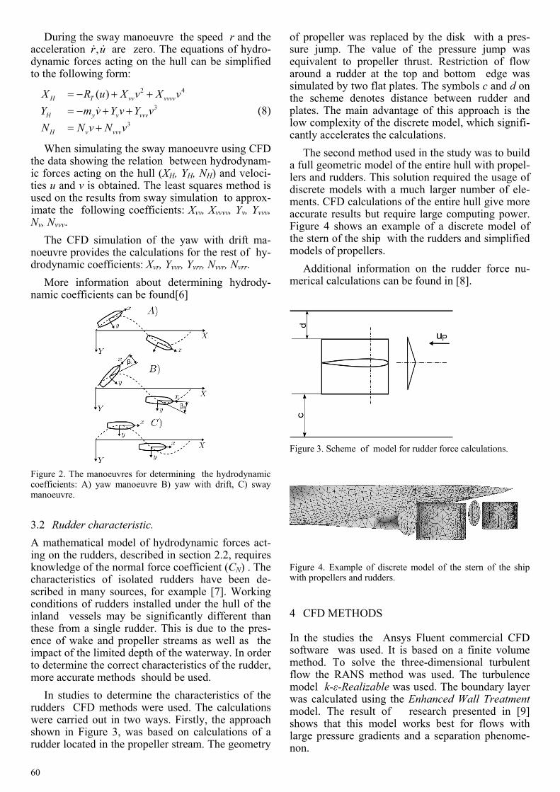
o determine the coefficients of hydrodynamic in-teractions it is necessary to have a database con-taining the values of the hydrodynamic forces and the corresponding to them values of velocity (u,v,r) and the acceleration ( , ,u v r ) of the ship. One way to obtain such a database is to simulate with help of CFD software the series of tests (manoeuvres): yaw , yaw with drift, sway test. Figure (2) shows the tra-jectory of a ship during these manoeuvres.

The values of the added mass (mx ,my,) coeffi-cients , added inertia (jzz) coefficient and the ship resistance (RT(u)) can be obtained on the basis of empirical methods or CFD calculations.

During the yaw manoeuvre the ship transverse velocity v and acceleration v are zero. The equa-tions of the hydrodynamic forces acting on the hull can be simplified to the following form:

2

3

3

( )H x T rr

H x r rrr

H zz r rrr

X m u R X rY m ur Y r Y rN j r N N r

u

r

= − − += − + += − + +

(7)

In the results of CFD simulation of the yaw ma-noeuvre the relation between hydrodynamic forces and moment (XH, YH , NH) and velocity u, r, and ac-celeration u is obtained. The least squares method can be used on the results from yaw simulation to approximate the following coefficients: Xrr, Yr, Yrrr, Nr, Nrrr .

60

During the sway manoeuvre the speed r and the acceleration ,r u are zero. The equations of hydro-dynamic forces acting on the hull can be simplified to the following form:

2 4

3

3

( )H T vv vvvv

H y v vvv

H v vvv

X R X v X vY m v Y v Y vN N v

u

N v

= − + += − + += +

(8)

When simulating the sway manoeuvre using CFD the data showing the relation between hydrodynam-ic forces acting on the hull (XH, YH, NH) and veloci-ties u and v is obtained. The least squares method is used on the results from sway simulation to approx-imate the following coefficients: Xvv, Xvvvv, Yv, Yvvv, Nv, Nvvv.

The CFD simulation of the yaw with drift ma-noeuvre provides the calculations for the rest of hy-drodynamic coefficients: Xvr, Yvvr, Yvrr, Nvvr, Nvrr.

More information about determining hydrody-namic coefficients can be found[6]

Figure 2. The manoeuvres for determining the hydrodynamic coefficients: A) yaw manoeuvre B) yaw with drift, C) sway manoeuvre.

3.2 Rudder characteristic. A mathematical model of hydrodynamic forces act-ing on the rudders, described in section 2.2, requires knowledge of the normal force coefficient (CN) . The characteristics of isolated rudders have been de-scribed in many sources, for example [7]. Working conditions of rudders installed under the hull of the inland vessels may be significantly different than these from a single rudder. This is due to the pres-ence of wake and propeller streams as well as the impact of the limited depth of the waterway. In order to determine the correct characteristics of the rudder, more accurate methods should be used.

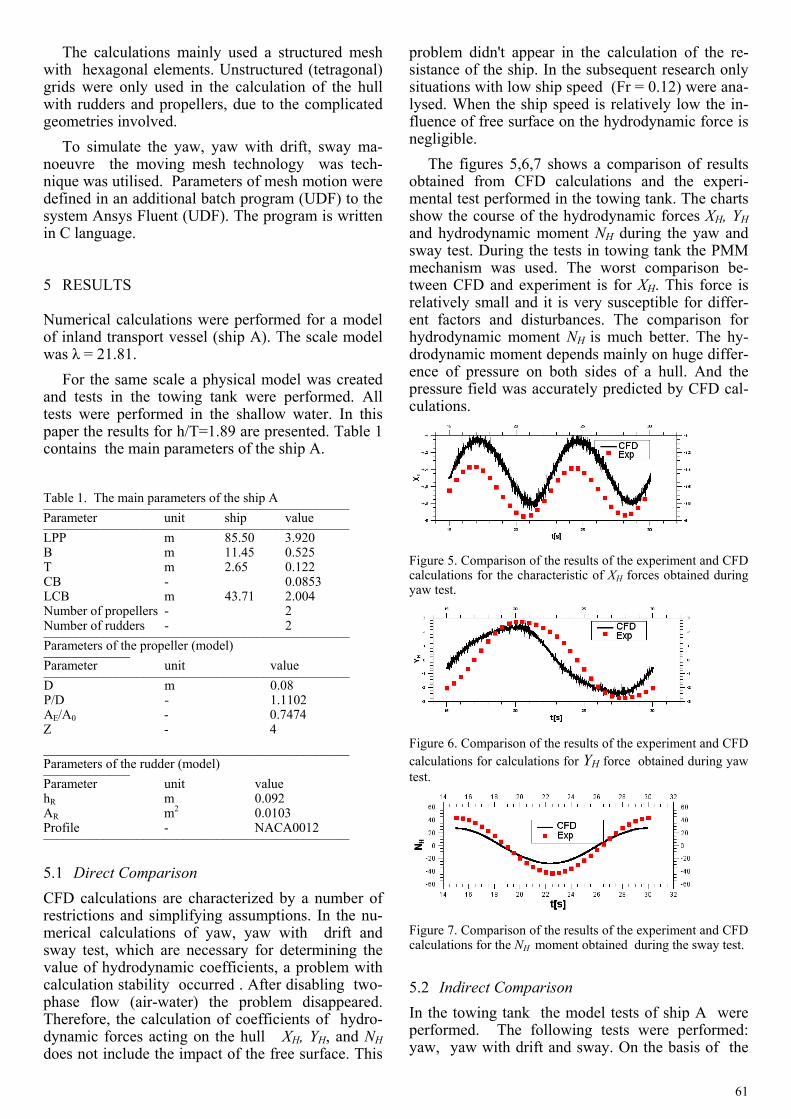
In studies to determine the characteristics of the rudders CFD methods were used. The calculations were carried out in two ways. Firstly, the approach shown in Figure 3, was based on calculations of a rudder located in the propeller stream. The geometry

of propeller was replaced by the disk with a pres-sure jump. The value of the pressure jump was equivalent to propeller thrust. Restriction of flow around a rudder at the top and bottom edge was simulated by two flat plates. The symbols c and d on the scheme denotes distance between rudder and plates. The main advantage of this approach is the low complexity of the discrete model, which signifi-cantly accelerates the calculations.

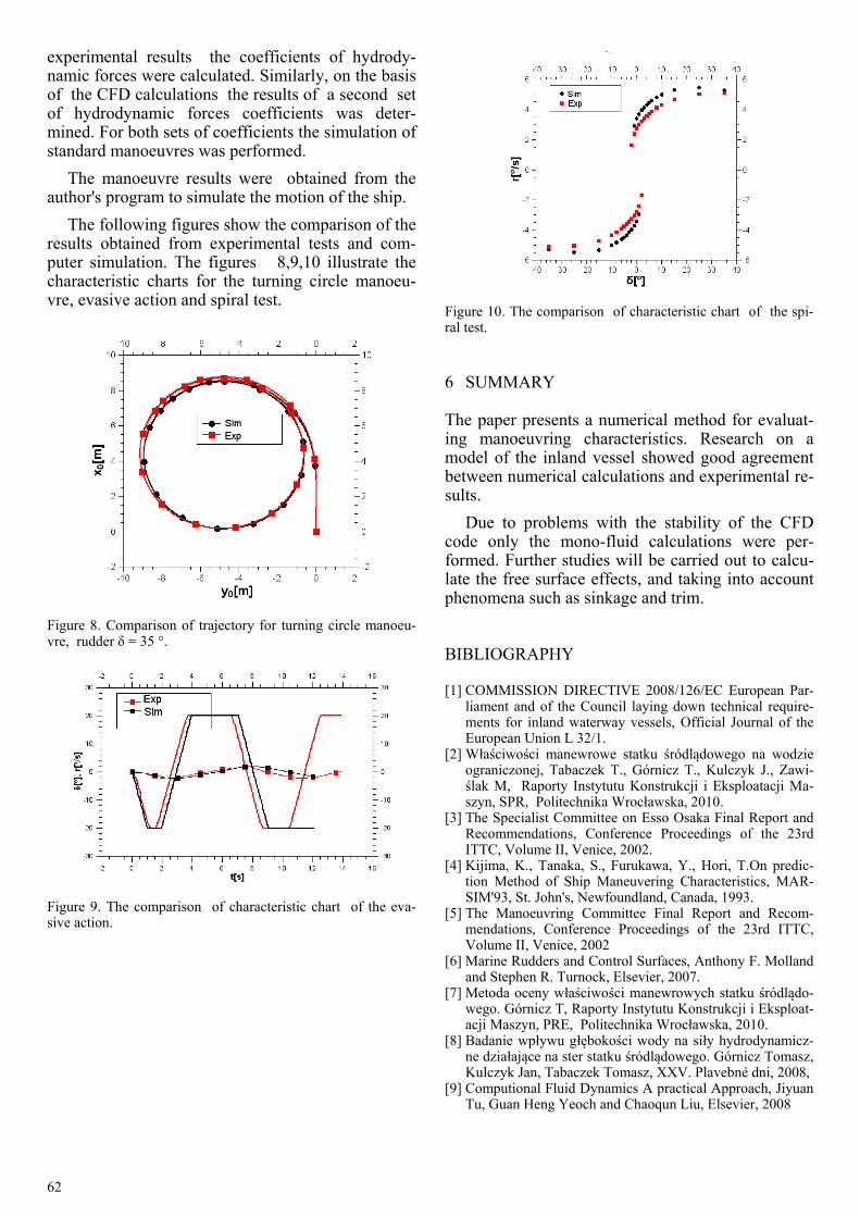
The second method used in the study was to build a full geometric model of the entire hull with propel-lers and rudders. This solution required the usage of discrete models with a much larger number of ele-ments. CFD calculations of the entire hull give more accurate results but require large computing power. Figure 4 shows an example of a discrete model of the stern of the ship with the rudders and simplified models of propellers.

Additional information on the rudder force nu-merical calculations can be found in [8].

Figure 3. Scheme of model for rudder force calculations.

Figure 4. Example of discrete model of the stern of the ship with propellers and rudders.

4 CFD METHODS

In the studies the Ansys Fluent commercial CFD software was used. It is based on a finite volume method. To solve the three-dimensional turbulent flow the RANS method was used. The turbulence model k-ε-Realizable was used. The boundary layer was calculated using the Enhanced Wall Treatment model. The result of research presented in [9] shows that this model works best for flows with large pressure gradients and a separation phenome-non.

61

The calculations mainly used a structured mesh with hexagonal elements. Unstructured (tetragonal) grids were only used in the calculation of the hull with rudders and propellers, due to the complicated geometries involved.

To simulate the yaw, yaw with drift, sway ma-noeuvre the moving mesh technology was tech-nique was utilised. Parameters of mesh motion were defined in an additional batch program (UDF) to the system Ansys Fluent (UDF). The program is written in C language.

5 RESULTS

Numerical calculations were performed for a model of inland transport vessel (ship A). The scale model was λ = 21.81.

For the same scale a physical model was created and tests in the towing tank were performed. All tests were performed in the shallow water. In this paper the results for h/T=1.89 are presented. Table 1 contains the main parameters of the ship A. Table 1. The main parameters of the ship A ______________________________________________ Parameter unit ship value ______________________________________________ LPP m 85.50 3.920 B m 11.45 0.525 T m 2.65 0.122 CB - 0.0853 LCB m 43.71 2.004 Number of propellers - 2 Number of rudders - 2 ______________________________________________ Parameters of the propeller (model) _____________ Parameter unit value ______________________________________________ D m 0.08 P/D - 1.1102 AE/A0 - 0.7474 Z - 4 ______________________________________________ Parameters of the rudder (model) _____________ Parameter unit value hR m 0.092 AR m2 0.0103 Profile - NACA0012 ______________________________________________

5.1 Direct Comparison CFD calculations are characterized by a number of restrictions and simplifying assumptions. In the nu-merical calculations of yaw, yaw with drift and sway test, which are necessary for determining the value of hydrodynamic coefficients, a problem with calculation stability occurred . After disabling two-phase flow (air-water) the problem disappeared. Therefore, the calculation of coefficients of hydro-dynamic forces acting on the hull XH, YH, and NH does not include the impact of the free surface. This

problem didn't appear in the calculation of the re-sistance of the ship. In the subsequent research only situations with low ship speed (Fr = 0.12) were ana-lysed. When the ship speed is relatively low the in-fluence of free surface on the hydrodynamic force is negligible.

The figures 5,6,7 shows a comparison of results obtained from CFD calculations and the experi-mental test performed in the towing tank. The charts show the course of the hydrodynamic forces XH, YH and hydrodynamic moment NH during the yaw and sway test. During the tests in towing tank the PMM mechanism was used. The worst comparison be-tween CFD and experiment is for XH. This force is relatively small and it is very susceptible for differ-ent factors and disturbances. The comparison for hydrodynamic moment NH is much better. The hy-drodynamic moment depends mainly on huge differ-ence of pressure on both sides of a hull. And the pressure field was accurately predicted by CFD cal-culations.

Figure 5. Comparison of the results of the experiment and CFD calculations for the characteristic of XH forces obtained during yaw test.

Figure 6. Comparison of the results of the experiment and CFD calculations for calculations for YH force obtained during yaw test.

Figure 7. Comparison of the results of the experiment and CFD calculations for the NH moment obtained during the sway test.

5.2 Indirect Comparison In the towing tank the model tests of ship A were performed. The following tests were performed: yaw, yaw with drift and sway. On the basis of the

62

experimental results the coefficients of hydrody-namic forces were calculated. Similarly, on the basis of the CFD calculations the results of a second set of hydrodynamic forces coefficients was deter-mined. For both sets of coefficients the simulation of standard manoeuvres was performed.

The manoeuvre results were obtained from the author's program to simulate the motion of the ship.

The following figures show the comparison of the results obtained from experimental tests and com-puter simulation. The figures 8,9,10 illustrate the characteristic charts for the turning circle manoeu-vre, evasive action and spiral test.

Figure 8. Comparison of trajectory for turning circle manoeu-vre, rudder δ = 35 °.

Figure 9. The comparison of characteristic chart of the eva-sive action.

Figure 10. The comparison of characteristic chart of the spi-ral test.

6 SUMMARY

The paper presents a numerical method for evaluat-ing manoeuvring characteristics. Research on a model of the inland vessel showed good agreement between numerical calculations and experimental re-sults.

Due to problems with the stability of the CFD code only the mono-fluid calculations were per-formed. Further studies will be carried out to calcu-late the free surface effects, and taking into account phenomena such as sinkage and trim.

BIBLIOGRAPHY

[1] COMMISSION DIRECTIVE 2008/126/EC European Par-liament and of the Council laying down technical require-ments for inland waterway vessels, Official Journal of the European Union L 32/1.

[2] Właściwości manewrowe statku śródlądowego na wodzie ograniczonej, Tabaczek T., Górnicz T., Kulczyk J., Zawi-ślak M, Raporty Instytutu Konstrukcji i Eksploatacji Ma-szyn, SPR, Politechnika Wrocławska, 2010.

[3] The Specialist Committee on Esso Osaka Final Report and Recommendations, Conference Proceedings of the 23rd ITTC, Volume II, Venice, 2002.

[4] Kijima, K., Tanaka, S., Furukawa, Y., Hori, T.On predic-tion Method of Ship Maneuvering Characteristics, MAR-SIM'93, St. John's, Newfoundland, Canada, 1993.

[5] The Manoeuvring Committee Final Report and Recom-mendations, Conference Proceedings of the 23rd ITTC, Volume II, Venice, 2002

[6] Marine Rudders and Control Surfaces, Anthony F. Molland and Stephen R. Turnock, Elsevier, 2007.

[7] Metoda oceny właściwości manewrowych statku śródlądo-wego. Górnicz T, Raporty Instytutu Konstrukcji i Eksploat-acji Maszyn, PRE, Politechnika Wrocławska, 2010.

[8] Badanie wpływu głębokości wody na siły hydrodynamicz-ne działające na ster statku śródlądowego. Górnicz Tomasz, Kulczyk Jan, Tabaczek Tomasz, XXV. Plavebné dni, 2008,

[9] Computional Fluid Dynamics A practical Approach, Jiyuan Tu, Guan Heng Yeoch and Chaoqun Liu, Elsevier, 2008