Application of data mining techniques

for energy modeling of HVAC sub-systems

Mathieu Le Cam1, Radu Zmeureanu1, and Ahmed Daoud2 1 Center for Zero Energy Building Studies, Department of Building, Civil, and Environmental

Engineering, Concordia University, Montreal, Canada 2 Laboratoire des technologies de l’énergie, Institut de recherche d’Hydro-Québec,

Shawinigan, Canada

Abstract

The Building Automation Systems (BAS) installed in commercial and

institutional buildings collects a very large amount of data. These meas-

urements present a gold mine of information which could be used for

better understanding of the actual building operation and performance,

or for fault detection. This study presents practical use of data mining to

extract information from BAS measurements, for development of inverse

models of building energy performance. The case study results show that

the target variable (the building demand for chilled water) depends on

the supply air temperature, humidity and enthalpy in the air-handling unit

(AHU), the cooling coil valve modulation in both AHUs, and outside air

enthalpy. About 75% of the variability of the dataset can be explained by

using only four principal components calculated from the original da-

taset. The clustering analysis revealed that four daily profiles could de-

scribe the chilled water daily use in summer and autumn seasons.

1 Introduction

The notion of data mining refers to the action of finding and extracting useful patterns in data.

Data mining is one specific step of the methodology of Knowledge Discovery in Databases

(KDD) mentioned in Fayyad et al. (1996). It comes along with data selection, preprocessing,

transformation and interpretation; these five main steps reshape the data from the original meas-

urements to the extraction and visualization of knowledge. The concept of data mining is closely

related to diverse fields such as artificial intelligence, machine learning statistics and database

systems. The five steps of the methodology are briefly explained below based on Fayyad et al.

(1996) and Kamath (2009). Some examples of application in HVAC systems are also presented.

Selection: From raw to target data

It may happen that the amount of data available is so huge that it can lead to difficulties in

managing, understanding and performing further operation on data, in addition to the increase

of the computing time for analysis. It is therefore useful to reduce the size of the dataset by

using sampling technique. When sampling the data, the size is reduced by removing redundancy

and effort is made to keep the variability and the representativeness of the sample to the original

dataset.

Preprocessing: From target to preprocessed data

Data preprocessing is an important step which is often neglected. It covers data cleaning and

normalization. Data cleaning aims at solving problems of missing values or outliers as well as

noise in the dataset which frequently occurs with measurements from sensors. Different meth-

ods can be employed depending on the number of missing values in a row; a linear interpolation

can be used when the missing data account for less than half of a day. Values of previous days

can be copied and used to fill in the dataset. Data collected through the BAS contain diverse

type of measurements, such as temperature, air flow rate or equipment status of operation, for

instance. In order to compare the different variables on an equal footing, data are normalized.

Transformation: From preprocessed to transformed data

The purpose of this is to reduce the dimension of the dataset; two different approaches exist:

feature selection and feature transformation.

The Feature selection approach consists in keeping only the relevant variables, called

predictors or regressors, for the modelling and prediction of selected target variable. For in-

stance, in Kusiak et al. (2010) a boosting tree algorithm is used to select the relevant variables

to model and minimize the energy used to condition an office building.

In the Feature transformation approach, the original variables are projected into an-

other mathematical space of lower dimension, which still describes the data with a good repre-

sentativeness. The Principal Component Analysis (PCA) is one transformation technique that

transforms the original regressors into a reduced number of independent features: the principal

components. For instance, Dunia et al. (1996) and Yi & Chen (2007) used PCA for faulty sen-

sors detection in variable air volume systems. Temporal data mining refers to the extraction

from time-dependent measurements, which is the normal case in HVAC system analysis. The

specific issues faced in temporal data mining are detailed in Antunes & Oliveira (2001). For

instance, data transformation could refer to the projection of measurements from the time-do-

main to the frequency domain.

Data mining: From transformed data to patterns

The data mining covers five main techniques used for description and prediction which are

detailed in Kamath (2009); their potential use in HVAC systems field is shortly described.

Anomaly detection is the identification of unusual data points, based on classification,

clustering, nearest neighbor, statistical techniques, information theory or even spectral methods;

a survey has been performed by Chandola et al. (2009) listing and explaining these different

techniques employed for anomaly detection. For instance, in O'Neill et al. (2013), statistical 𝑇2

and Q tests were used to detect an anomalous event by comparing measurements and predic-

tions; PCA was previously employed to reduce the dimension size.

Association rule learning searches for possible hidden relationships between variables.

For instance, in Yu et al. (2012), association and correlation rules were extracted from building

operational data; they revealed an issue in the operation strategy causing a waste of energy in

the air conditioning system and possible faults in equipment.

Clustering analysis identifies groups in the dataset by using their similarity without any

prior knowledge. For instance, clustering analysis can be used to identify the building energy

use daily profiles, which are grouped based on their pattern similarity. The main clusters can be

identified as well as the typical profile for each class for further operation strategy planning. In

Seem (2005), a modified agglomerative hierarchical clustering algorithm is used to group the

daily energy consumption profiles and analyse their similarity in terms of day-type. The purpose

is then to use that knowledge to perform forecasts or to detect abnormal energy consumption.

In West et al. (2011), a clustering algorithm was employed along with a technique based on

information theory for automated fault detection.

Classification is a prediction technique, which is employed to sort the data into previ-

ously known classes. It can be used to model and predict a categorical variable, which takes a

limited number of fixed values such as a system operation. In the previous example of clusters

of the typical daily profiles, a classification technique can be then used to predict in which class

would be the next profile. For instance, in Li et al. (2010), a classification technique is used to

predict the daily electric consumption profile.

Regression analysis is another prediction technique used to model the relationship be-

tween one or several dependent variable and one or several independent variables. Regression

techniques are similar to the classification techniques in their use, but they are applied to con-

tinuous variables, such as energy used, instead of categorical variables. A large number of stud-

ies have been conducted in the use of regression techniques to the prediction of building energy

performance, like in Reddy & Claridge (1994) and Feinberg & Genethliou (2005).

Interpretation: From patterns to knowledge

Summarization technique provides a compact representation of the dataset, including visuali-

zation and report generation.

Discussion

Data mining techniques are used for two main purposes which are prediction and description.

Since the extraction of information from patterns cannot be performed directly, the previous

steps have to be conducted to reduce the size of the dataset, clean the data and reduce the number

of dimensions by removing some feature variables. The important issue in data mining is the

way the problem of concern is defined and presented: how to reshape and pre-process the data

so that they would have the appropriate frame to provide interesting results. For instance, when

analysing the energy demand of a building, it could be more interesting to perform the analysis

on the daily profiles of selected variables rather than on one-value measurement.

Over the past few decades, only a few studies have been conducted on the use of data

mining for building energy performance analysis and prediction. With the increasing availabil-

ity of measurements from BAS, there is a great potential in the use of these techniques for better

understanding of the actual building operation and performance. They can be used in fault de-

tection, energy usage forecasting or even optimization of HVAC system operation (e.g., set

points) to minimize energy consumption or peak demand.

2 Case study

Target variable

The building case study is the Research Center for Structural Genomics of Concordia Univer-

sity, located in Montreal, further called Genome building. The dataset used was collected at a

15-min time step through the BAS system; it includes measurements of (1) the chilled water

flow rate entering the building from a central cooling plant; (2) the thermodynamic properties

of air, hot water and chilled water, and supply and return air flow rates in the two main AHUs;

and (3) the indoor air temperature and supply air flow rate in rooms. In this case study, the target

variable is the whole building chilled water flow rate during the summer and autumn of 2013.

The following sections present the application of some data mining techniques for data prepro-

cessing, transformation and mining to select the most appropriate regressors for the future pre-

diction of the target variable.

Data exploration

This sub-section presents some statistical information about the target variable and the available

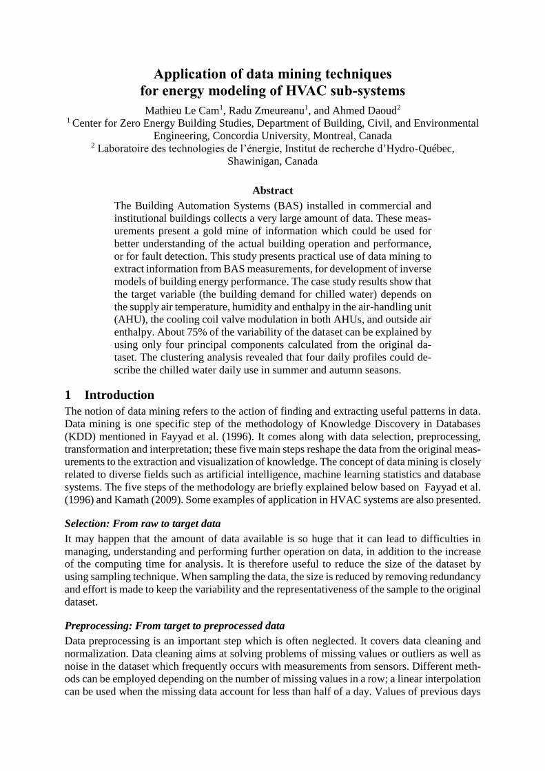
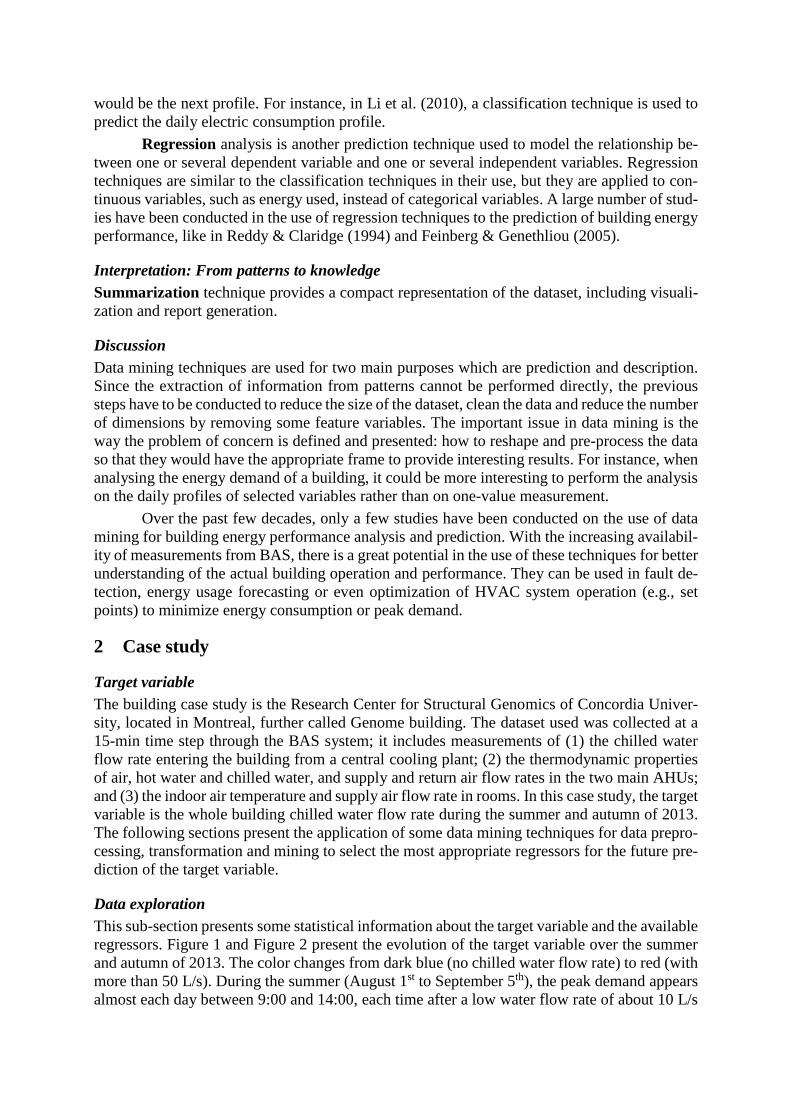
regressors. Figure 1 and Figure 2 present the evolution of the target variable over the summer

and autumn of 2013. The color changes from dark blue (no chilled water flow rate) to red (with

more than 50 L/s). During the summer (August 1st to September 5th), the peak demand appears

almost each day between 9:00 and 14:00, each time after a low water flow rate of about 10 L/s

over a few hours. The following hours, the water flow rate stays almost constant at around 30

L/s. In autumn, the chilled water flow rate is significant in the afternoon and remains around 10

L/s in the morning; after mid-October, it stays around 10 L/s for 24 hours.

Figure 1 Carpet plot of the chilled water flow rate in summer and fall of 2013

Figure 2 3D view of the variation of chilled water flow rate in summer and fall of 2013

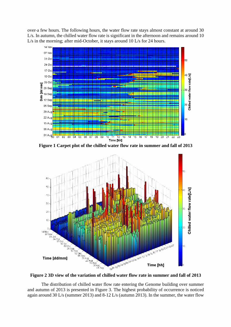
The distribution of chilled water flow rate entering the Genome building over summer

and autumn of 2013 is presented in Figure 3. The highest probability of occurrence is noticed

again around 30 L/s (summer 2013) and 8-12 L/s (autumn 2013). In the summer, the water flow

rate varies between 20 and 40 L/s; however, a small secondary water flow rate peak of around

12 L/s is also noticed with a relatively significant frequency of occurrence.

Figure 3: Chilled water flow rate distribution

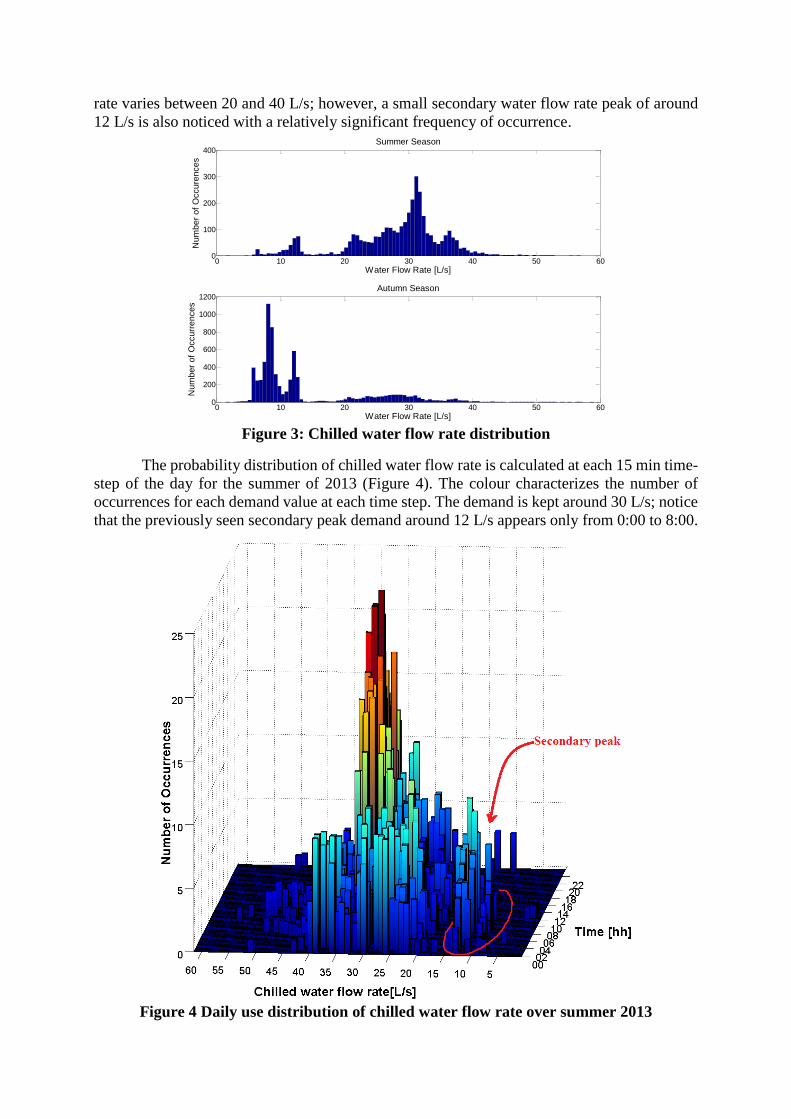
The probability distribution of chilled water flow rate is calculated at each 15 min time-

step of the day for the summer of 2013 (Figure 4). The colour characterizes the number of

occurrences for each demand value at each time step. The demand is kept around 30 L/s; notice

that the previously seen secondary peak demand around 12 L/s appears only from 0:00 to 8:00.

Figure 4 Daily use distribution of chilled water flow rate over summer 2013

0 10 20 30 40 50 600

100

200

300

400

Num

ber

of

Occure

nces

Water Flow Rate [L/s]

Summer Season

0 10 20 30 40 50 600

200

400

600

800

1000

1200

Num

ber

of

Occurr

ences

Water Flow Rate [L/s]

Autumn Season

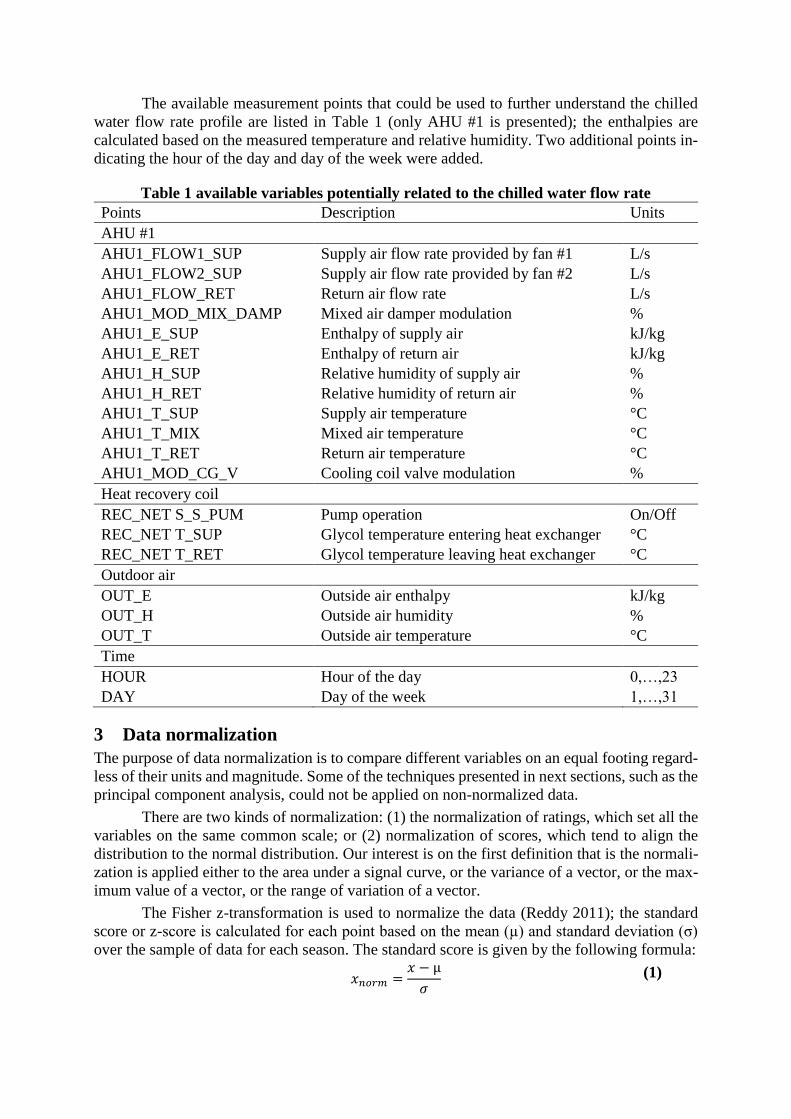
The available measurement points that could be used to further understand the chilled

water flow rate profile are listed in Table 1 (only AHU #1 is presented); the enthalpies are

calculated based on the measured temperature and relative humidity. Two additional points in-

dicating the hour of the day and day of the week were added.

Table 1 available variables potentially related to the chilled water flow rate

Points Description Units

AHU #1

AHU1_FLOW1_SUP Supply air flow rate provided by fan #1 L/s

AHU1_FLOW2_SUP Supply air flow rate provided by fan #2 L/s

AHU1_FLOW_RET Return air flow rate L/s

AHU1_MOD_MIX_DAMP Mixed air damper modulation %

AHU1_E_SUP Enthalpy of supply air kJ/kg

AHU1_E_RET Enthalpy of return air kJ/kg

AHU1_H_SUP Relative humidity of supply air %

AHU1_H_RET Relative humidity of return air %

AHU1_T_SUP Supply air temperature °C

AHU1_T_MIX Mixed air temperature °C

AHU1_T_RET Return air temperature °C

AHU1_MOD_CG_V Cooling coil valve modulation %

Heat recovery coil

REC_NET S_S_PUM Pump operation On/Off

REC_NET T_SUP Glycol temperature entering heat exchanger °C

REC_NET T_RET Glycol temperature leaving heat exchanger °C

Outdoor air

OUT_E Outside air enthalpy kJ/kg

OUT_H Outside air humidity %

OUT_T Outside air temperature °C

Time

HOUR Hour of the day 0,…,23

DAY Day of the week 1,…,31

3 Data normalization

The purpose of data normalization is to compare different variables on an equal footing regard-

less of their units and magnitude. Some of the techniques presented in next sections, such as the

principal component analysis, could not be applied on non-normalized data.

There are two kinds of normalization: (1) the normalization of ratings, which set all the

variables on the same common scale; or (2) normalization of scores, which tend to align the

distribution to the normal distribution. Our interest is on the first definition that is the normali-

zation is applied either to the area under a signal curve, or the variance of a vector, or the max-

imum value of a vector, or the range of variation of a vector.

The Fisher z-transformation is used to normalize the data (Reddy 2011); the standard

score or z-score is calculated for each point based on the mean (µ) and standard deviation (σ)

over the sample of data for each season. The standard score is given by the following formula:

𝑥𝑛𝑜𝑟𝑚 =𝑥 − µ

𝜎 (1)

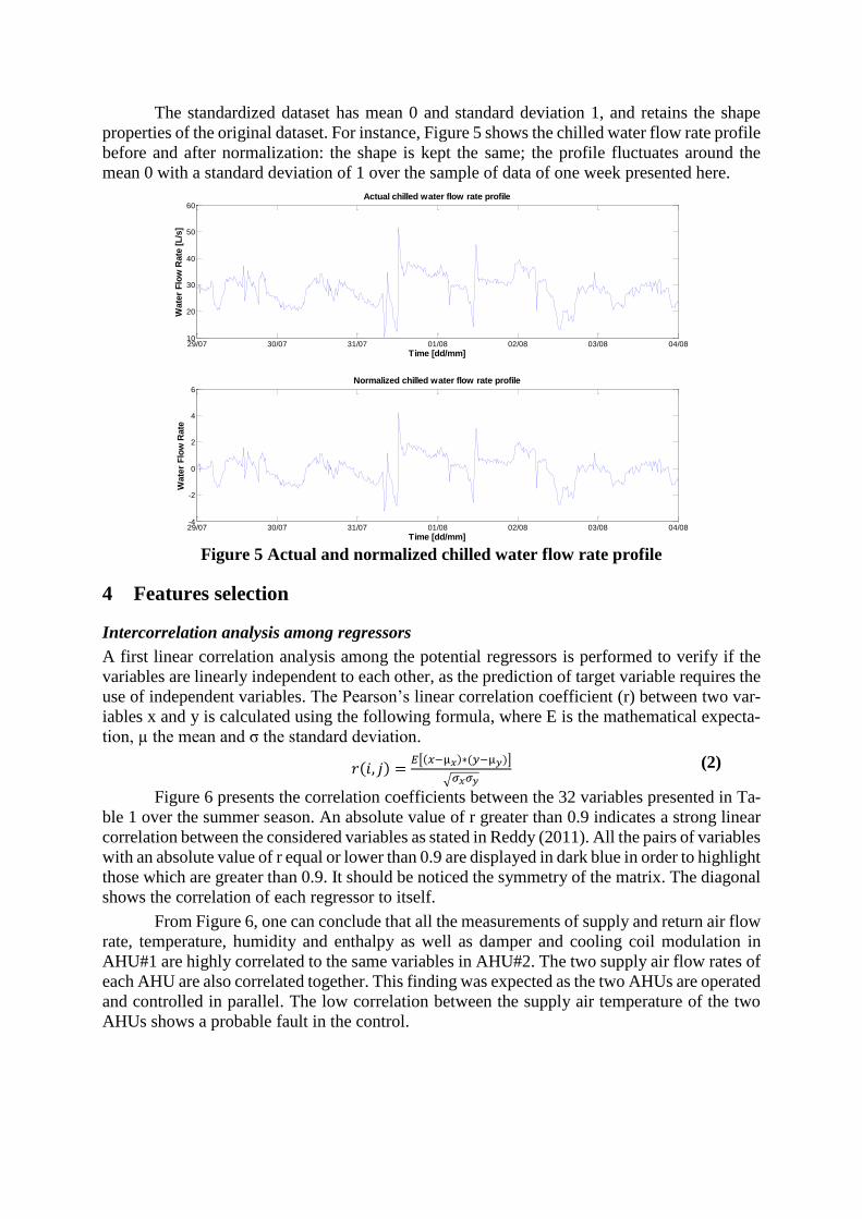
The standardized dataset has mean 0 and standard deviation 1, and retains the shape

properties of the original dataset. For instance, Figure 5 shows the chilled water flow rate profile

before and after normalization: the shape is kept the same; the profile fluctuates around the

mean 0 with a standard deviation of 1 over the sample of data of one week presented here.

Figure 5 Actual and normalized chilled water flow rate profile

4 Features selection

Intercorrelation analysis among regressors

A first linear correlation analysis among the potential regressors is performed to verify if the

variables are linearly independent to each other, as the prediction of target variable requires the

use of independent variables. The Pearson’s linear correlation coefficient (r) between two var-

iables x and y is calculated using the following formula, where E is the mathematical expecta-

tion, µ the mean and σ the standard deviation.

𝑟(𝑖, 𝑗) =𝐸[(𝑥−µ𝑥)∗(𝑦−µ𝑦)]

√𝜎𝑥𝜎𝑦 (2)

Figure 6 presents the correlation coefficients between the 32 variables presented in Ta-

ble 1 over the summer season. An absolute value of r greater than 0.9 indicates a strong linear

correlation between the considered variables as stated in Reddy (2011). All the pairs of variables

with an absolute value of r equal or lower than 0.9 are displayed in dark blue in order to highlight

those which are greater than 0.9. It should be noticed the symmetry of the matrix. The diagonal

shows the correlation of each regressor to itself.

From Figure 6, one can conclude that all the measurements of supply and return air flow

rate, temperature, humidity and enthalpy as well as damper and cooling coil modulation in

AHU#1 are highly correlated to the same variables in AHU#2. The two supply air flow rates of

each AHU are also correlated together. This finding was expected as the two AHUs are operated

and controlled in parallel. The low correlation between the supply air temperature of the two

AHUs shows a probable fault in the control.

29/07 30/07 31/07 01/08 02/08 03/08 04/0810

20

30

40

50

60

Time [dd/mm]

Wate

r F

low

Rate

[L

/s]

Actual chilled water flow rate profile

29/07 30/07 31/07 01/08 02/08 03/08 04/08-4

-2

0

2

4

6

Time [dd/mm]

Wate

r F

low

Rate

Normalized chilled water flow rate profile

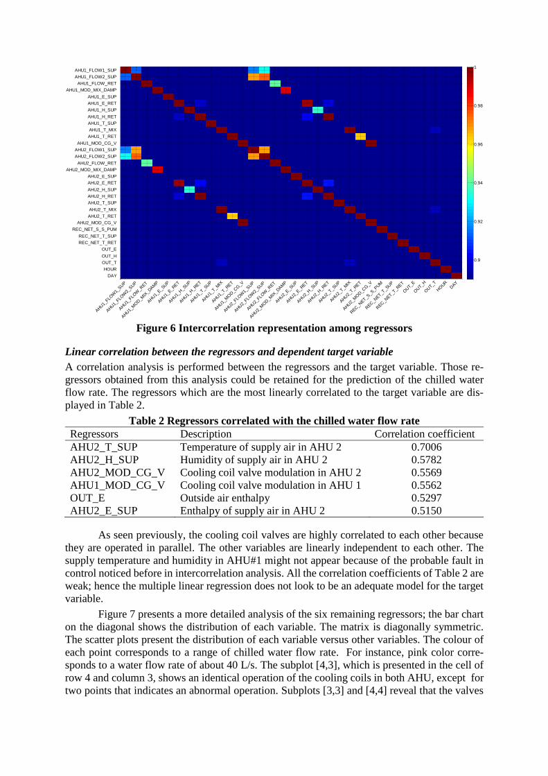
Figure 6 Intercorrelation representation among regressors

Linear correlation between the regressors and dependent target variable

A correlation analysis is performed between the regressors and the target variable. Those re-

gressors obtained from this analysis could be retained for the prediction of the chilled water

flow rate. The regressors which are the most linearly correlated to the target variable are dis-

played in Table 2.

Table 2 Regressors correlated with the chilled water flow rate

Regressors Description Correlation coefficient

AHU2_T_SUP Temperature of supply air in AHU 2 0.7006

AHU2_H_SUP Humidity of supply air in AHU 2 0.5782

AHU2_MOD_CG_V Cooling coil valve modulation in AHU 2 0.5569

AHU1_MOD_CG_V Cooling coil valve modulation in AHU 1 0.5562

OUT_E Outside air enthalpy 0.5297

AHU2_E_SUP Enthalpy of supply air in AHU 2 0.5150

As seen previously, the cooling coil valves are highly correlated to each other because

they are operated in parallel. The other variables are linearly independent to each other. The

supply temperature and humidity in AHU#1 might not appear because of the probable fault in

control noticed before in intercorrelation analysis. All the correlation coefficients of Table 2 are

weak; hence the multiple linear regression does not look to be an adequate model for the target

variable.

Figure 7 presents a more detailed analysis of the six remaining regressors; the bar chart

on the diagonal shows the distribution of each variable. The matrix is diagonally symmetric.

The scatter plots present the distribution of each variable versus other variables. The colour of

each point corresponds to a range of chilled water flow rate. For instance, pink color corre-

sponds to a water flow rate of about 40 L/s. The subplot [4,3], which is presented in the cell of

row 4 and column 3, shows an identical operation of the cooling coils in both AHU, except for

two points that indicates an abnormal operation. Subplots [3,3] and [4,4] reveal that the valves

AHU1_

FLOW

1_SUP

AHU1_

FLOW

2_SUP

AHU1_

FLOW

_RET

AHU1_

MO

D_M

IX_D

AM

P

AHU1_

E_S

UP

AHU1_

E_R

ET

AHU1_

H_S

UP

AHU1_

H_R

ET

AHU1_

T_SUP

AHU1_

T_MIX

AHU1_

T_RET

AHU1_

MO

D_C

G_V

AHU2_

FLOW

1_SUP

AHU2_

FLOW

2_SUP

AHU2_

FLOW

_RET

AHU2_

MO

D_M

IX_D

AM

P

AHU2_

E_S

UP

AHU2_

E_R

ET

AHU2_

H_S

UP

AHU2_

H_R

ET

AHU2_

T_SUP

AHU2_

T_MIX

AHU2_

T_RET

AHU2_

MO

D_C

G_V

REC

_NET_S

_S_P

UM

REC

_NET_T

_SUP

REC

_NET_T

_RET

OUT_

E

OUT_

H

OUT_

T

HO

UR

DAY

AHU1_FLOW1_SUP

AHU1_FLOW2_SUP

AHU1_FLOW_RET

AHU1_MOD_MIX_DAMP

AHU1_E_SUP

AHU1_E_RET

AHU1_H_SUP

AHU1_H_RET

AHU1_T_SUP

AHU1_T_MIX

AHU1_T_RET

AHU1_MOD_CG_V

AHU2_FLOW1_SUP

AHU2_FLOW2_SUP

AHU2_FLOW_RET

AHU2_MOD_MIX_DAMP

AHU2_E_SUP

AHU2_E_RET

AHU2_H_SUP

AHU2_H_RET

AHU2_T_SUP

AHU2_T_MIX

AHU2_T_RET

AHU2_MOD_CG_V

REC_NET_S_S_PUM

REC_NET_T_SUP

REC_NET_T_RET

OUT_E

OUT_H

OUT_T

HOUR

DAY

0.9

0.92

0.94

0.96

0.98

1

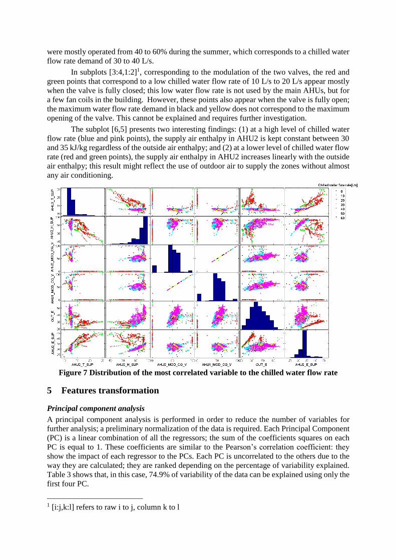
were mostly operated from 40 to 60% during the summer, which corresponds to a chilled water

flow rate demand of 30 to 40 L/s.

In subplots [3:4,1:2]1, corresponding to the modulation of the two valves, the red and

green points that correspond to a low chilled water flow rate of 10 L/s to 20 L/s appear mostly

when the valve is fully closed; this low water flow rate is not used by the main AHUs, but for

a few fan coils in the building. However, these points also appear when the valve is fully open;

the maximum water flow rate demand in black and yellow does not correspond to the maximum

opening of the valve. This cannot be explained and requires further investigation.

The subplot [6,5] presents two interesting findings: (1) at a high level of chilled water

flow rate (blue and pink points), the supply air enthalpy in AHU2 is kept constant between 30

and 35 kJ/kg regardless of the outside air enthalpy; and (2) at a lower level of chilled water flow

rate (red and green points), the supply air enthalpy in AHU2 increases linearly with the outside

air enthalpy; this result might reflect the use of outdoor air to supply the zones without almost

any air conditioning.

Figure 7 Distribution of the most correlated variable to the chilled water flow rate

5 Features transformation

Principal component analysis

A principal component analysis is performed in order to reduce the number of variables for

further analysis; a preliminary normalization of the data is required. Each Principal Component

(PC) is a linear combination of all the regressors; the sum of the coefficients squares on each

PC is equal to 1. These coefficients are similar to the Pearson’s correlation coefficient: they

show the impact of each regressor to the PCs. Each PC is uncorrelated to the others due to the

way they are calculated; they are ranked depending on the percentage of variability explained.

Table 3 shows that, in this case, 74.9% of variability of the data can be explained using only the

first four PC.

1 [i:j,k:l] refers to raw i to j, column k to l

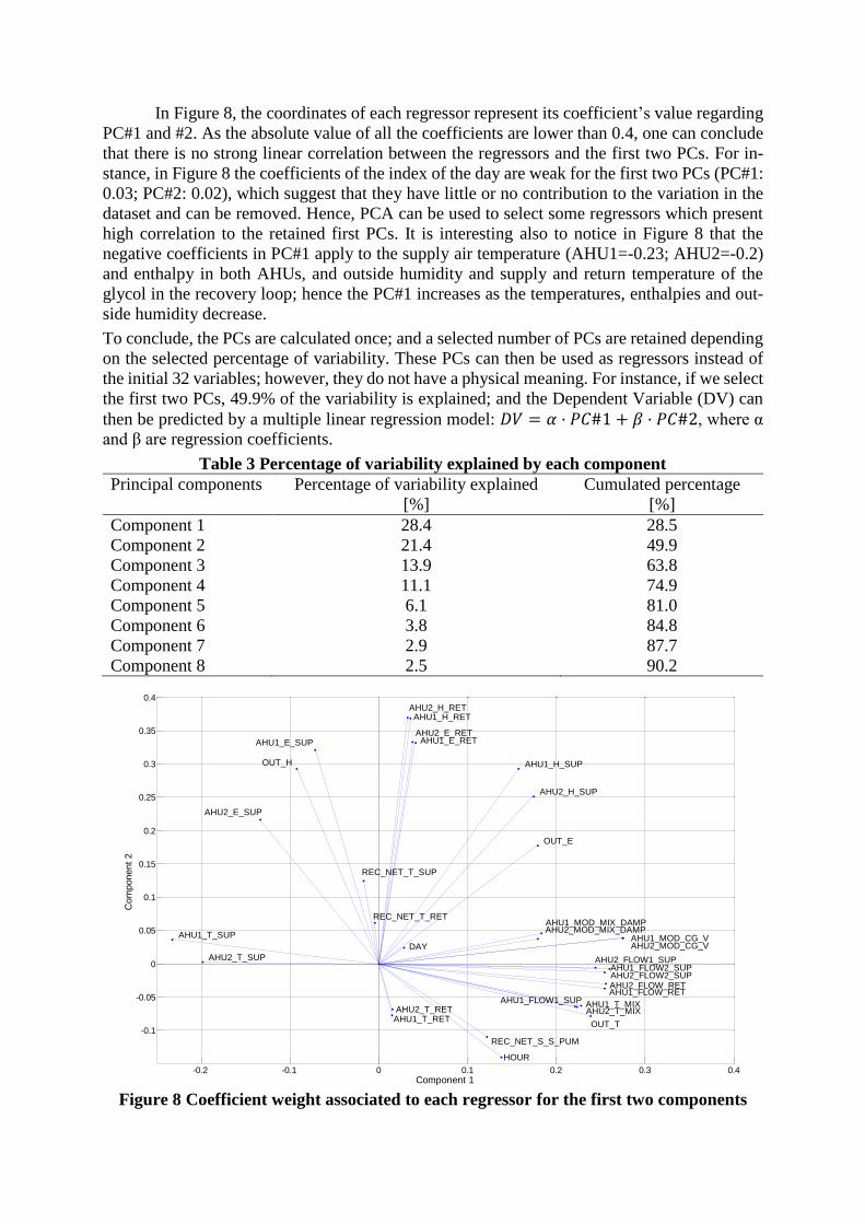
In Figure 8, the coordinates of each regressor represent its coefficient’s value regarding

PC#1 and #2. As the absolute value of all the coefficients are lower than 0.4, one can conclude

that there is no strong linear correlation between the regressors and the first two PCs. For in-

stance, in Figure 8 the coefficients of the index of the day are weak for the first two PCs (PC#1:

0.03; PC#2: 0.02), which suggest that they have little or no contribution to the variation in the

dataset and can be removed. Hence, PCA can be used to select some regressors which present

high correlation to the retained first PCs. It is interesting also to notice in Figure 8 that the

negative coefficients in PC#1 apply to the supply air temperature (AHU1=-0.23; AHU2=-0.2)

and enthalpy in both AHUs, and outside humidity and supply and return temperature of the

glycol in the recovery loop; hence the PC#1 increases as the temperatures, enthalpies and out-

side humidity decrease.

To conclude, the PCs are calculated once; and a selected number of PCs are retained depending

on the selected percentage of variability. These PCs can then be used as regressors instead of

the initial 32 variables; however, they do not have a physical meaning. For instance, if we select

the first two PCs, 49.9% of the variability is explained; and the Dependent Variable (DV) can

then be predicted by a multiple linear regression model: 𝐷𝑉 = 𝛼 · 𝑃𝐶#1 + 𝛽 · 𝑃𝐶#2, where α

and β are regression coefficients.

Table 3 Percentage of variability explained by each component

Principal components Percentage of variability explained

[%]

Cumulated percentage

[%]

Component 1 28.4 28.5

Component 2 21.4 49.9

Component 3 13.9 63.8

Component 4 11.1 74.9

Component 5 6.1 81.0

Component 6 3.8 84.8

Component 7 2.9 87.7

Component 8 2.5 90.2

Figure 8 Coefficient weight associated to each regressor for the first two components

-0.2 -0.1 0 0.1 0.2 0.3 0.4

-0.1

-0.05

0

0.05

0.1

0.15

0.2

0.25

0.3

0.35

0.4

AHU1_FLOW1_SUP

AHU1_FLOW2_SUP

AHU1_FLOW_RET

AHU1_MOD_MIX_DAMP

AHU1_E_SUP AHU1_E_RET

AHU1_H_SUP

AHU1_H_RET

AHU1_T_SUP

AHU1_T_MIX

AHU1_T_RET

AHU1_MOD_CG_V

AHU2_FLOW1_SUP

AHU2_FLOW2_SUPAHU2_FLOW_RET

AHU2_MOD_MIX_DAMP

AHU2_E_SUP

AHU2_E_RET

AHU2_H_SUP

AHU2_H_RET

AHU2_T_SUP

AHU2_T_MIXAHU2_T_RET

AHU2_MOD_CG_V

REC_NET_S_S_PUM

REC_NET_T_SUP

REC_NET_T_RET

OUT_E

OUT_H

OUT_T

HOUR

DAY

Component 1

Com

ponent

2

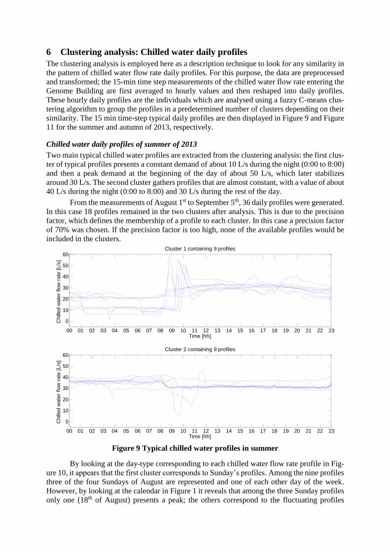
6 Clustering analysis: Chilled water daily profiles

The clustering analysis is employed here as a description technique to look for any similarity in

the pattern of chilled water flow rate daily profiles. For this purpose, the data are preprocessed

and transformed; the 15-min time step measurements of the chilled water flow rate entering the

Genome Building are first averaged to hourly values and then reshaped into daily profiles.

These hourly daily profiles are the individuals which are analysed using a fuzzy C-means clus-

tering algorithm to group the profiles in a predetermined number of clusters depending on their

similarity. The 15 min time-step typical daily profiles are then displayed in Figure 9 and Figure

11 for the summer and autumn of 2013, respectively.

Chilled water daily profiles of summer of 2013

Two main typical chilled water profiles are extracted from the clustering analysis: the first clus-

ter of typical profiles presents a constant demand of about 10 L/s during the night (0:00 to 8:00)

and then a peak demand at the beginning of the day of about 50 L/s, which later stabilizes

around 30 L/s. The second cluster gathers profiles that are almost constant, with a value of about

40 L/s during the night (0:00 to 8:00) and 30 L/s during the rest of the day.

From the measurements of August 1st to September 5th, 36 daily profiles were generated.

In this case 18 profiles remained in the two clusters after analysis. This is due to the precision

factor, which defines the membership of a profile to each cluster. In this case a precision factor

of 70% was chosen. If the precision factor is too high, none of the available profiles would be

included in the clusters.

Figure 9 Typical chilled water profiles in summer

By looking at the day-type corresponding to each chilled water flow rate profile in Fig-

ure 10, it appears that the first cluster corresponds to Sunday’s profiles. Among the nine profiles

three of the four Sundays of August are represented and one of each other day of the week.

However, by looking at the calendar in Figure 1 it reveals that among the three Sunday profiles

only one (18th of August) presents a peak; the others correspond to the fluctuating profiles

00 01 02 03 04 05 06 07 08 09 10 11 12 13 14 15 16 17 18 19 20 21 22 23

0

10

20

30

40

50

60

Time [hh]

Chill

ed w

ate

r flow

rate

[L/s

]

Cluster 1 containing 9 profiles

00 01 02 03 04 05 06 07 08 09 10 11 12 13 14 15 16 17 18 19 20 21 22 23

0

10

20

30

40

50

60

Time [hh]

Chill

ed w

ate

r flow

rate

[L/s

]

Cluster 2 containing 9 profiles

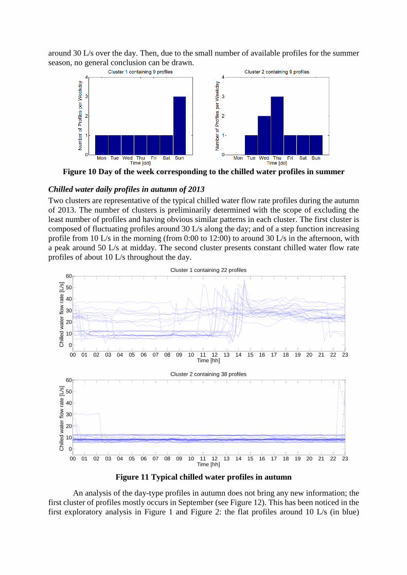
around 30 L/s over the day. Then, due to the small number of available profiles for the summer

season, no general conclusion can be drawn.

Figure 10 Day of the week corresponding to the chilled water profiles in summer

Chilled water daily profiles in autumn of 2013

Two clusters are representative of the typical chilled water flow rate profiles during the autumn

of 2013. The number of clusters is preliminarily determined with the scope of excluding the

least number of profiles and having obvious similar patterns in each cluster. The first cluster is

composed of fluctuating profiles around 30 L/s along the day; and of a step function increasing

profile from 10 L/s in the morning (from 0:00 to 12:00) to around 30 L/s in the afternoon, with

a peak around 50 L/s at midday. The second cluster presents constant chilled water flow rate

profiles of about 10 L/s throughout the day.

Figure 11 Typical chilled water profiles in autumn

An analysis of the day-type profiles in autumn does not bring any new information; the

first cluster of profiles mostly occurs in September (see Figure 12). This has been noticed in the

first exploratory analysis in Figure 1 and Figure 2: the flat profiles around 10 L/s (in blue)

00 01 02 03 04 05 06 07 08 09 10 11 12 13 14 15 16 17 18 19 20 21 22 23

0

10

20

30

40

50

60

Time [hh]

Chill

ed w

ate

r flow

rate

[L/s

]

Cluster 1 containing 22 profiles

00 01 02 03 04 05 06 07 08 09 10 11 12 13 14 15 16 17 18 19 20 21 22 23

0

10

20

30

40

50

60

Time [hh]

Chill

ed w

ate

r flow

rate

[L/s

]

Cluster 2 containing 38 profiles

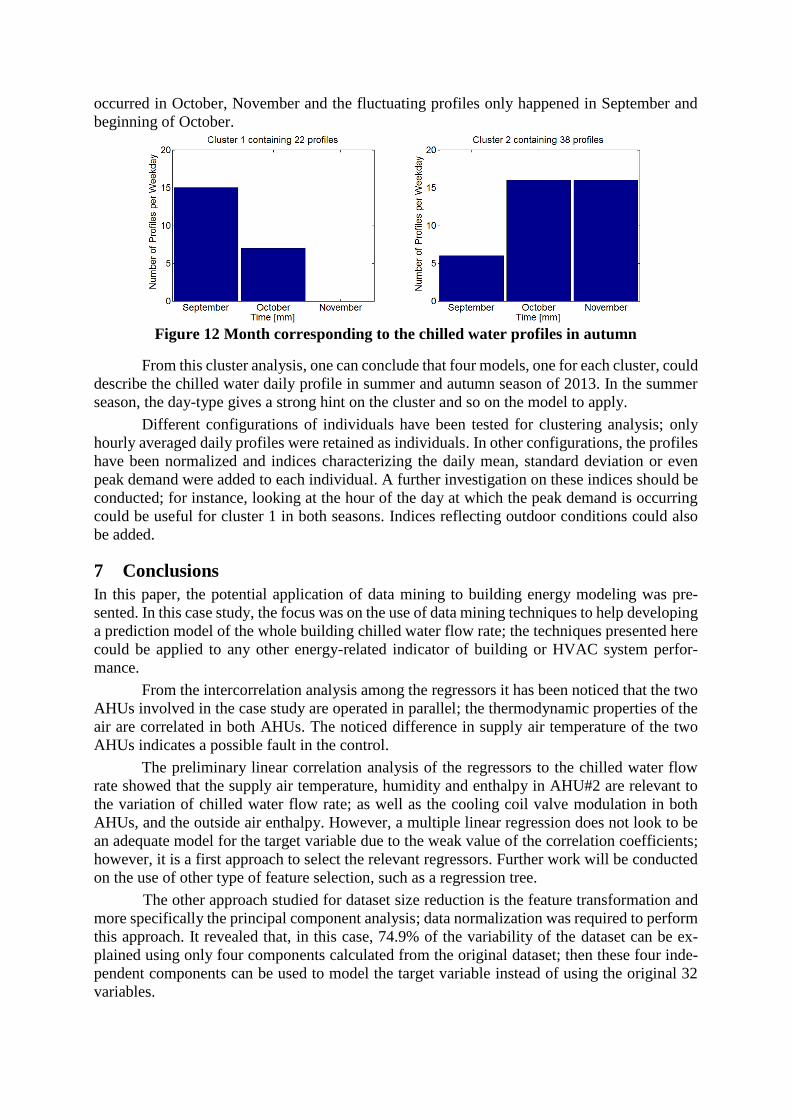
occurred in October, November and the fluctuating profiles only happened in September and

beginning of October.

Figure 12 Month corresponding to the chilled water profiles in autumn

From this cluster analysis, one can conclude that four models, one for each cluster, could

describe the chilled water daily profile in summer and autumn season of 2013. In the summer

season, the day-type gives a strong hint on the cluster and so on the model to apply.

Different configurations of individuals have been tested for clustering analysis; only

hourly averaged daily profiles were retained as individuals. In other configurations, the profiles

have been normalized and indices characterizing the daily mean, standard deviation or even

peak demand were added to each individual. A further investigation on these indices should be

conducted; for instance, looking at the hour of the day at which the peak demand is occurring

could be useful for cluster 1 in both seasons. Indices reflecting outdoor conditions could also

be added.

7 Conclusions

In this paper, the potential application of data mining to building energy modeling was pre-

sented. In this case study, the focus was on the use of data mining techniques to help developing

a prediction model of the whole building chilled water flow rate; the techniques presented here

could be applied to any other energy-related indicator of building or HVAC system perfor-

mance.

From the intercorrelation analysis among the regressors it has been noticed that the two

AHUs involved in the case study are operated in parallel; the thermodynamic properties of the

air are correlated in both AHUs. The noticed difference in supply air temperature of the two

AHUs indicates a possible fault in the control.

The preliminary linear correlation analysis of the regressors to the chilled water flow

rate showed that the supply air temperature, humidity and enthalpy in AHU#2 are relevant to

the variation of chilled water flow rate; as well as the cooling coil valve modulation in both

AHUs, and the outside air enthalpy. However, a multiple linear regression does not look to be

an adequate model for the target variable due to the weak value of the correlation coefficients;

however, it is a first approach to select the relevant regressors. Further work will be conducted

on the use of other type of feature selection, such as a regression tree.

The other approach studied for dataset size reduction is the feature transformation and

more specifically the principal component analysis; data normalization was required to perform

this approach. It revealed that, in this case, 74.9% of the variability of the dataset can be ex-

plained using only four components calculated from the original dataset; then these four inde-

pendent components can be used to model the target variable instead of using the original 32

variables.

The clustering analysis revealed that four models could describe the chilled water daily

profile in summer and autumn seasons of 2013. The summer day-types give a strong infor-

mation on the cluster and so the model to apply. For the autumn other explanatory parameters

should be investigated. Then, benchmarking models for each cluster can be developed to predict

the daily profile of chilled water flow rate.

Further work will investigate the application of other data mining techniques for anom-

aly detection or prediction such as classification and regression.

8 Acknowledgments

The authors acknowledge the financial support from NSERC Smart Net-Zero Energy Building

Strategic Research Network and the Faculty of Engineering and Computer Science of Concor-

dia University and Hydro-Quebec.

9 References

Antunes, C. M. & Oliveira, A. L. 2001. Temporal data mining: An overview. KDD Workshop

on Temporal Data Mining.

Chandola, V., Banerjee, A. & Kumar, V. 2009. Anomaly detection: A survey. ACM Computing

Surveys (CSUR) 41(3): 15.

Dunia, R., Qin, S. J., Edgar, T. F. & McAvoy, T. J. 1996. Identification of faulty sensors using

principal component analysis. AIChE Journal 42(10): 2797-2812.

Fayyad, U., Piatetsky-Shapiro, G. & Smyth, P. 1996. From data mining to knowledge discovery

in databases. AI magazine 17(3): 37.

Feinberg, E. A. & Genethliou, D. 2005. Load forecasting. Applied Mathematics for

Restructured Electric Power Systems, Springer US: 269-285.

Kamath, C. 2009. Scientific data mining: a practical perspective, Siam.

Kusiak, A., Li, M. & Tang, F. 2010. Modeling and optimization of HVAC energy consumption.

Applied Energy 87(10): 3092-3102.

Li, X., Bowers, C. P. & Schnier, T. 2010. Classification of energy consumption in buildings

with outlier detection. Industrial Electronics, IEEE Transactions on 57(11): 3639-3644.

O'Neill, Z., Pang, X., Shashanka, M., Haves, P. & Bailey, T. 2013. Model-based real-time

whole building energy performance monitoring and diagnostics. Journal of Building

Performance Simulation 7(2): 1-17.

Reddy, T. & Claridge, D. 1994. Using synthetic data to evaluate multiple regression and

principal component analyses for statistical modeling of daily building energy

consumption. Energy and Buildings 21(1): 35-44.

Reddy, T. A. 2011. Applied data analysis and modeling for energy engineers and scientists,

Springer.

Seem, J. E. 2005. Pattern recognition algorithm for determining days of the week with similar

energy consumption profiles. Energy and buildings 37(2): 127-139.

West, S. R., Guo, Y., Wang, X. R., Wall, J., Soebarto, V., Bennetts, H., Bannister, P., Thomas,

P. & Leach, D. 2011. Automated fault detection and diagnosis of HVAC subsystems

using statistical machine learning. Proceedings of Building Simulation 2011. Sydney,

Australia, IBPSA: 2659-2665.

Yi, X. & Chen, Y. 2007. Sensor fault detection and diagnosis for VAV system based on principal

component analysis. Proceedings of Building Simulation 2007. Beijing, China, IBPSA:

1313-1318.

Yu, Z. J., Haghighat, F., Fung, B. & Zhou, L. 2012. A novel methodology for knowledge

discovery through mining associations between building operational data. Energy and

Buildings 47: 430-440.