Application of Decline Curve Analysis To Estimate Recovery ... · Application of Decline Curve Analysis To Estimate Recovery Factors for Carbon Dioxide Enhanced Oil Recovery By Hossein

Application of Decline Curve Analysis To Estimate Recovery Factors for Carbon Dioxide Enhanced Oil Recovery

By Hossein Jahediesfanjani

Chapter C ofThree Approaches forEstimating Recovery Factors inCarbon Dioxide Enhanced Oil RecoveryMahendra K. Verma, Editor

Scientific Investigations Report 2017–5062–C

U.S. Department of the InteriorU.S. Geological Survey

U.S. Department of the InteriorRYAN K. ZINKE, Secretary

U.S. Geological SurveyWilliam H. Werkheiser, Acting Director

U.S. Geological Survey, Reston, Virginia: 2017

For more information on the USGS—the Federal source for science about the Earth, its natural and living resources, natural hazards, and the environment—visit https://www.usgs.gov or call 1–888–ASK–USGS.

For an overview of USGS information products, including maps, imagery, and publications, visit https://store.usgs.gov.

Any use of trade, firm, or product names is for descriptive purposes only and does not imply endorsement by the U.S. Government.

Although this information product, for the most part, is in the public domain, it also may contain copyrighted materials as noted in the text. Permission to reproduce copyrighted items must be secured from the copyright owner.

Suggested citation:Jahediesfanjani, Hossein, 2017, Application of decline curve analysis to estimate recovery factors for carbon dioxide enhanced oil recovery, chap. C of Verma, M.K., ed., Three approaches for estimating recovery factors in carbon dioxide enhanced oil recovery: U.S. Geological Survey Scientific Investigations Report 2017–5062, p. C1–C20, https://doi.org/10.3133/sir20175062C.

ISSN 2328-0328 (online)

https://www.usgs.gov

https://store.usgs.gov

https://doi.org/10.3133/sir20175062C

iii

Contents

Background..................................................................................................................................................C1Basis for Decline Curve Analysis ................................................................................................................1Case Study ......................................................................................................................................................2Discussion .......................................................................................................................................................5References Cited............................................................................................................................................5Appendix C1. Decline Curve Analysis of Selected Reservoirs ...........................................................9

Figures

C1. Semi-log plot of the oil production rate versus the oil production time for the San Andres Limestone in the Sable oil field in the west Texas section of the Permian Basin Province, showing the decline trends for both the waterflood and the carbon dioxide enhanced oil recovery (CO2-EOR) phases .........................................................................................................C3

C2. Graph of the oil production rate versus the cumulative oil production for the San Andres Limestone in the Sable oil field, Texas, showing the decline trends for both the waterflood and the carbon dioxide enhanced oil recovery (CO2-EOR) phases ......................................................................................4

C3. Bar graph showing the number of studied reservoirs having values of additional oil recovery factors due to carbon dioxide enhanced oil recovery (CO2-EOR) in five different ranges ...............................................................4

C1–1 to C1–15. Graphs of the oil production rate versus the cumulative oil production showing the decline trends for both the waterflood and the carbon dioxide enhanced oil recovery (CO2-EOR) phases for the—

C1–1. San Andres Limestone in the Sable oil field, Texas .................................13 C1–2. Weber Sandstone in the Rangely oil field, Colorado ...............................14 C1–3. Tensleep Formation in the Lost Soldier oil field, Wyoming ....................14 C1–4. Madison Formation in the Lost Soldier oil field, Wyoming .....................15 C1–5. San Andres Limestone in the Wasson oil field, Texas ............................15 C1–6. Clear Fork Group in the Wasson oil field, Texas.......................................16 C1–7. Thirtyone Formation in the Dollarhide oil field, Texas .............................16 C1–8. Clear Fork Group in the Dollarhide oil field, Texas ...................................17 C1–9. “Canyon-age reservoir” in the Salt Creek oil field, Texas ......................17 C1–10. San Andres Limestone in the Seminole oil field, Texas ..........................18 C1–11. Sandstone of the Ramsey Member of the Bell Canyon

Formation in the Twofreds oil field, Texas .................................................18 C1–12. San Andres Limestone in the Vacuum oil field, New Mexico ................19 C1–13. San Andres Limestone in the Cedar Lake oil field, Texas .......................19 C1–14. San Andres Limestone in the North Hobbs oil field,

New Mexico ...................................................................................................20 C1–15. San Andres Limestone in the Yates oil field, Texas .................................20

iv

Tables

C1. Best match values of the initial oil production rate, the initial decline rate for oil production, and the corresponding coefficient of determination (R2) values for both waterflood and carbon dioxide enhanced oil recovery (CO2-EOR) decline periods of the studied reservoirs ..............................................................................C6

C2. Additional oil recovery factors estimated by using decline curve analysis for carbon dioxide enhanced oil recovery (CO2-EOR) projects in 15 selected reservoirs .......................................................................................................................................7

Chapter C. Application of Decline Curve Analysis To Estimate Recovery Factors for Carbon Dioxide Enhanced Oil Recovery

By Hossein Jahediesfanjani1

1Lynxnet LLC, under contract to the U.S. Geological Survey.

BackgroundIn the decline curve analysis (DCA) method of estimating

recoverable hydrocarbon volumes, the analyst uses historical production data from a well, lease, group of wells (or pattern), or reservoir and plots production rates against time or cumu-lative production for the analysis. The DCA of an individual well is founded on the same basis as the fluid-flow principles that are used for pressure-transient analysis of a single well in a reservoir domain (Fetkovich, 1987; Fetkovich and others, 1987) and therefore can provide scientifically reasonable and accurate results. However, when used for a group of wells, a lease, or a reservoir, the DCA becomes more of an empirical method. Plots from the DCA reflect the reservoir response to the oil withdrawal (or production) under the prevailing operating and reservoir conditions, and they continue to be good tools for estimating recoverable hydrocarbon volumes and future production rates. For predicting the total recov-erable hydrocarbon volume, the DCA results can help the analyst to evaluate the reservoir performance under any of the three phases of reservoir productive life—primary, secondary (waterflood), or tertiary (enhanced oil recovery) phases—so long as the historical production data are sufficient to establish decline trends at the end of the three phases.

Basis for Decline Curve AnalysisThe DCA method is used to predict the future oil pro-

duction rate of an oil-producing well or reservoir. Theoreti-cally, according to this method, the oil production rate for a given entity will first reach its maximum output and then decline according to the following generalized relationship (Fetkovich, 1987):

qq

bD t

q

ii

b= +−

( )11

whereis the time-dependent oil production rrate,

in barrels per day (bbl/day);is the initial oil pqi rroduction rate, in barrels

per day;is the initial decliDi nne rate per year;represents the degree of curvature of tb hhe

shape of the decline trend, which is dimensionless; andd

is the oil production time, in years.t

(C1)

Theoretically, the parameters, such as qi , Di , and b, have defined meanings only if equation C1 is applied for a single well that produces from a single reservoir under appropri-ate fluid-flow conditions. However, if equation C1 is applied to larger entities such as a number of wells, a reservoir, or a field, these parameters are only empirical and are obtained by a curve-fitting process. Practically, this equation represents three different types of declines depending on the value of b; namely, an exponential decline for b = 0, a hyperbolic decline for b > 0 and b < 1, and a harmonic decline for b = 1. On the basis of the explanations above and for the sake of simplicity, in many of the industrial applications of evaluating reservoir oil production decline, the value of b is often assumed to be zero, and, hence, equation C1 takes the form:

q q D ti i= −exp( ) (C2)

C2 Three Approaches for Estimating Recovery Factors in Carbon Dioxide Enhanced Oil Recovery

Equation C2 is rewritten in terms of cumulative oil pro-duction in the following form:

Q q qD

Q

i

i

=−( )

whereis the cumulative oil production, in barrells.

(C3)

These two equations, C2 and C3, were used for the analy-sis of oil production decline in this current study to determine the values of constants “Di” and “qi” in the above equations. For this purpose, these equations can be written as:

ln( ) ln( )q q D ti i= − (C4)

q q DQi i= − (C5)

On the basis of equation C4, plotting the oil production ate (q) versus production time (t) on a semi-log graph will esult in a straight line having an intercept equal to ln(qi) and slope equal to Di . Alternatively, on the basis of equation 5, plotting the oil production rate (q) versus cumulative oil roduction (Q) will result in a straight line having an intercept nd slope equal to qi and Di , respectively. After values are etermined for Di and qi , equations C4 and C5 are used to pre-ict the future oil production rate and the cumulative amount f recoverable oil, respectively. The current assessment meth-dology is designed to assess only the technically recoverable ydrocarbon for the carbon dioxide enhanced oil recovery CO2-EOR) application, implying no economic limit. If an conomic evaluation is required in the future, first an appropri-te economic hydrocarbon production rate (qec) in reservoir arrels per day (bbl/day) needs to be defined below which ydrocarbon production from a given reservoir is considered o be uneconomic. The magnitude of the introduced value of ec depends on each project configuration and specifications nd external factors such as hydrocarbon prices that vary from

rraCpaddooh(eabhtqaone project to another. After the value of qec is chosen, the field’s productive life ( )tec and total economically recoverable hydrocarbon volume ( )Qec can be calculated by applying the following equations:

tD

qqec

i

ec

i

= −

1 ln (C6)

QD

q qeci

i ec= − −( )1 (C7)

For a technically recoverable hydrocarbon volume, desig-nated as Qmax , the recovery factor (RF) under current produc-tion conditions is estimated from the following:

RF QOOIP

Q

max

max

= ×100

whereis the maximum cumulative oil

produuction, in barrels (bbl);is the original oil in placeOOIP ,, in stock tank

barrels (STB); andis the recovery factoRF rr, expressed as a

percentage.

(C8)

If an incremental recovery factor is required for any phase (that is, primary, secondary, or tertiary), it is determined as the total calculated RF at phase i minus the total calculated RF at the previous phase (i – 1):

RF RF RF

i

Incremental i i= − −1

whereis 1 for primary, 2 for seconddary, and 3 for

tertiary production.

(C9)

For example, if the reservoir is currently under CO2-EOR, which was initiated after a waterflood, the calculated RF at the current stage represents the total recovery, including all three stages of primary, waterflood, and CO2-EOR. Therefore, on the basis of equation C9, the additional recovery factor due to CO2-EOR is obtained by subtracting the calculated RF values of the waterflood from the RF value calculated for the CO2-EOR.

Case StudyThe Oil and Gas Journal’s 2012 survey of EOR projects

(Koottungal, 2012; Kuuskraa, 2012) indicated that about 123 CO2-EOR projects were active within the United States in 2012. Twenty-four fields (28 reservoirs) of these projects were initially selected for DCA. However, after the initial investigation, almost half of these projects were excluded from the DCA because they either did not develop long enough CO2-EOR decline periods appropriate for the DCA or were not in their decline phases yet. Data for the DCA were obtained from the comprehensive resource database (CRD), which was described by Carolus and others (in press); the CRD was developed from two proprietary databases by Nehring Associ-ates Inc. (2012) and IHS Inc. (2012) and provided adequate injection and production data for only 12 fields containing 15 reservoirs. Therefore, the DCA was successfully applied

Chapter C. Application of Decline Curve Analysis To Estimate Recovery Factors for CO2-EOR C3

only on these fields that have established a good CO2-EOR decline trend. The results of DCA on 15 reservoirs from these 12 fields are summarized in table C1 (tables follow the “References Cited”). The DCA for the Sable oil field in the west Texas section of the Permian Basin Province is presented here to show the procedure, and the details of the DCA for all the 15 reservoirs are provided in appendix C1. It is important to note that the Sable oil field was under a CO2-EOR opera-tion from 1984 to 2001 and hence was not an active CO2-EOR project in 2012. However, because it makes a great example of the application of DCA, this field is being analyzed and presented herein.

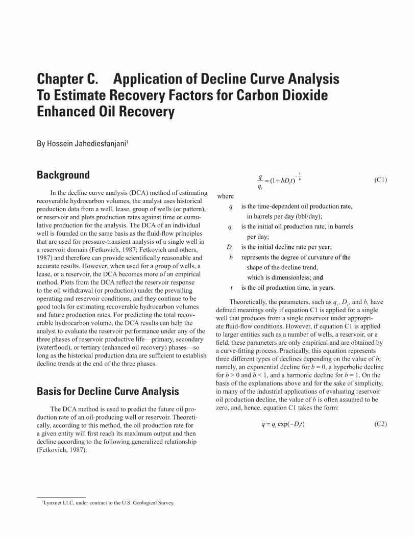
In order to present the DCA procedure and demonstrate its applicability in modeling both waterflood and CO2-EOR decline periods for the Sable oil field, two figures were gener-ated and are discussed. Figure C1 shows the semi-log plot of oil production rate versus production time for the Sable oil field. This graph shows that the oil production decline during waterflood that began in 1976 continued until 1984, when the CO2-EOR project was initiated. Because of CO2-EOR, the field production remained stable until 1993, when the produc-tion decline started again.

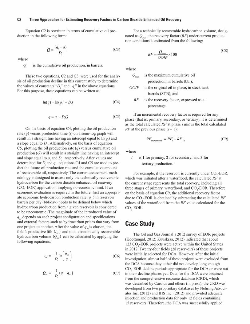
Figure C2 shows the oil production rate versus the cumu-lative oil production for the Sable oil field. As shown in the figure, the technically recoverable oil volume has increased from 9.85 million barrels (MMbbl) for the waterflood phase to 13.1 MMbbl for the CO2-EOR phase.

Figure C1. Semi-log plot of the oil production rate versus the oil production time for the San Andres Limestone in the Sable oil field in the west Texas section of the Permian Basin Province, showing the decline trends for both the waterflood and the carbon dioxide enhanced oil recovery (CO2-EOR) phases. Data are from IHS Inc. (2012). Terms used in the decline equations on the graph: Di = initial decline rate per year; q = oil production rate, in barrels per day (bbl/day); qi = initial oil production rate, in barrels per day (bbl/day); R2 = coefficient of determination; t = oil production time, in years.

The oil production data for DCA are from IHS Inc. (2012), and the calculated OOIP values are from the CRD (Carolus and others, in press), which is based on data from the Nehring Associates Inc. database (2012) and IHS Inc. (2012). Because the OOIP values from the CRD are proprietary, the OOIP values of reservoirs are reported qualitatively in table C2 and appendix C1 as small, medium, and large: a small OOIP is less than or equal to 100 MMbbl, a medium OOIP is between 100 and 1,000 MMbbl, and a large OOIP is larger than or equal to 1,000 MMbbl. The OOIP of the San Andres Limestone of the Sable oil field was estimated volumetrically to be less than 100 MMbbl, thus classifying the reservoir in the Sable field as a small reservoir. By applying equation C8, the calculated recovery factors are 27.2 and 36.2 percent for waterflood and CO2-EOR, respectively (table C2). On the basis of equation C9, the additional recovery-factor value due to CO2-EOR is 9.0 percent. A similar process has been repeated for the selected 14 reservoirs located in Colorado, Wyoming, and the Permian Basin of Texas and New Mexico that were under CO2-EOR in 2012.

The additional recoverable oil volumes for CO2-EOR in 15 selected reservoirs were estimated by using DCA. Recov-ery factors were calculated by dividing the recoverable oil vol-umes at the end of the waterflood and at the end of CO2-EOR by the OOIP of the individual reservoirs.

1958 1978 1998 2018 2038 2058 2078 2098

1

10

100

1,000

10,000

0 20 40 60 80 100 120 140

Oil p

rodu

ctio

n ra

te, i

n ba

rrel

s pe

r day

Oil production time, in years

Beginning of CO2-EOR: 1984

Beginning of waterflood decline: 1976

Beginning of CO2-EOR decline: 1993

Date

CO2-EOR Declineln(q) = ln(5,580) − 0.0627tR2 = 0.992qi = 5,580 bbl/dayDi = 0.0627/year

Waterflood Declineln(q) = ln(12,100) − 0.108tR2 = 0.990qi = 12,100 bbl/dayDi = 0.1080/year

EXPLANATION

Historical oil production

Waterflood decline trend—Dashed where extended

CO2-EOR decline trend—Dashed where extended


CO2-EOR Decliney = −182.4x + 2,390R2 = 0.99qi = 2,390 bbl/dayDi = 182.4/yearWaterflood Decline

y = −299.8x + 2,950R2 = 0.99qi = 2,950 bbl/dayDi = 299.8/year

200

400

600

800

1,000

1,200

1,400

1,600

1,800

0 2 4 6 8 10 12 14

Oil p

rodu

ctio

n ra

te, i

n ba

rrel

s pe

r day

Cumulative oil production, in millions of barrels


Q@(q=0) = 9.85 MMbbl Q@(q=0) = 13.1 MMbbl

0

EXPLANATION




Figure C2. Graph of the oil production rate versus the cumulative oil production for the San Andres Limestone in the Sable oil field, Texas, showing the decline trends for both the waterflood and the carbon dioxide enhanced oil recovery (CO2-EOR) phases. Data are from IHS Inc. (2012). Terms used in the decline equations on the graph: Di = initial decline rate per year; q = oil production rate, in barrels per day (bbl/day); qi = initial oil production rate, in barrels per day (bbl/day); Q = cumulative oil production, in millions of barrels (MMbbl); R2 = coefficient of determination; x = cumulative oil production in the trendline equation, in millions of barrels; y = oil production rate in the trendline equation, in barrels per day.

0

1

2

3

4

5

6

7

≥ 5 to 10 ≥ 10 to 15 ≥ 15 to 20 ≥ 20 to 25 ≥ 25

Num

ber o

f stu

died

pro

ject

s

Ranges of additional recovery-factor values for CO2-EOR, in percent

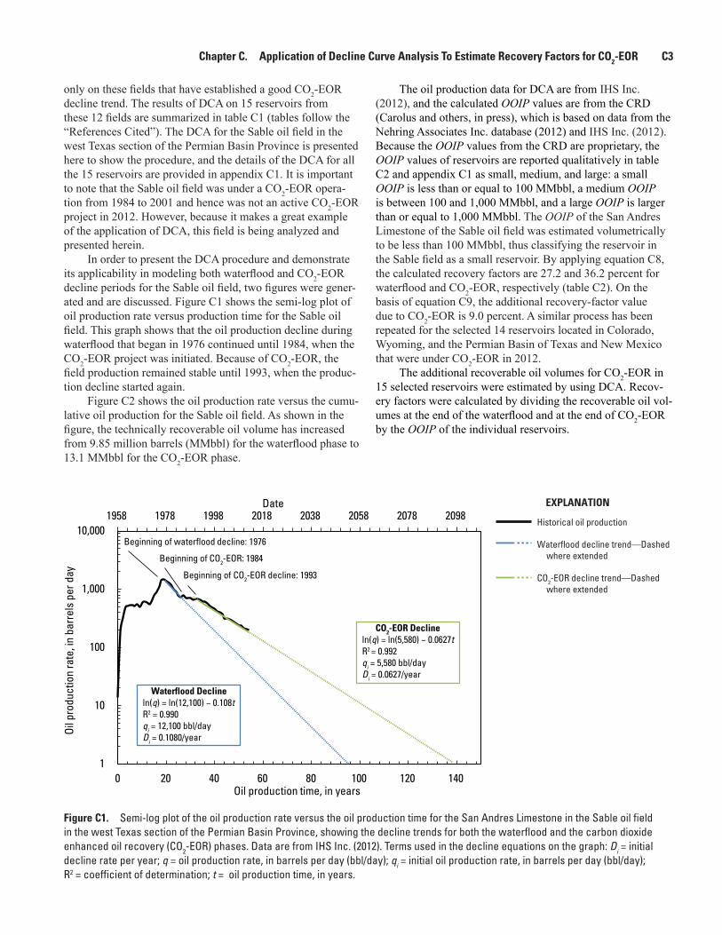
Figure C3. Bar graph showing the number of studied reservoirs having values of additional oil recovery factors due to carbon dioxide enhanced oil recovery (CO2-EOR) in five different ranges. Recovery-factor values estimated by decline curve analysis are from table C2.


DiscussionGenerally speaking, the DCA is utilized in this study as

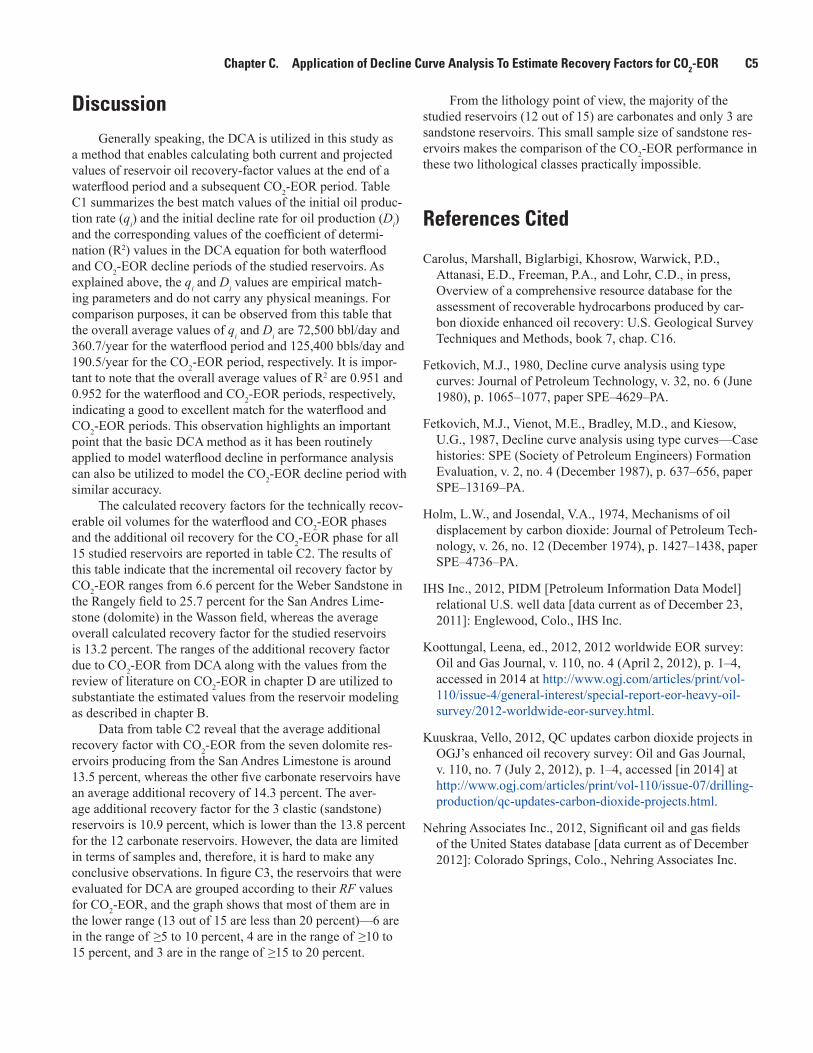
a method that enables calculating both current and projected values of reservoir oil recovery-factor values at the end of a waterflood period and a subsequent CO2-EOR period. Table C1 summarizes the best match values of the initial oil produc-tion rate (qi) and the initial decline rate for oil production (Di) and the corresponding values of the coefficient of determi-nation (R2) values in the DCA equation for both waterflood and CO2-EOR decline periods of the studied reservoirs. As explained above, the qi and Di values are empirical match-ing parameters and do not carry any physical meanings. For comparison purposes, it can be observed from this table that the overall average values of qi and Di are 72,500 bbl/day and 360.7/year for the waterflood period and 125,400 bbls/day and 190.5/year for the CO2-EOR period, respectively. It is impor-tant to note that the overall average values of R2 are 0.951 and 0.952 for the waterflood and CO2-EOR periods, respectively, indicating a good to excellent match for the waterflood and CO2-EOR periods. This observation highlights an important point that the basic DCA method as it has been routinely applied to model waterflood decline in performance analysis can also be utilized to model the CO2-EOR decline period with similar accuracy.

The calculated recovery factors for the technically recov-erable oil volumes for the waterflood and CO2-EOR phases and the additional oil recovery for the CO2-EOR phase for all 15 studied reservoirs are reported in table C2. The results of this table indicate that the incremental oil recovery factor by CO2-EOR ranges from 6.6 percent for the Weber Sandstone in the Rangely field to 25.7 percent for the San Andres Lime-stone (dolomite) in the Wasson field, whereas the average overall calculated recovery factor for the studied reservoirs is 13.2 percent. The ranges of the additional recovery factor due to CO2-EOR from DCA along with the values from the review of literature on CO2-EOR in chapter D are utilized to substantiate the estimated values from the reservoir modeling as described in chapter B.

Data from table C2 reveal that the average additional recovery factor with CO2-EOR from the seven dolomite res-ervoirs producing from the San Andres Limestone is around 13.5 percent, whereas the other five carbonate reservoirs have an average additional recovery of 14.3 percent. The aver-age additional recovery factor for the 3 clastic (sandstone) reservoirs is 10.9 percent, which is lower than the 13.8 percent for the 12 carbonate reservoirs. However, the data are limited in terms of samples and, therefore, it is hard to make any conclusive observations. In figure C3, the reservoirs that were evaluated for DCA are grouped according to their RF values for CO2-EOR, and the graph shows that most of them are in the lower range (13 out of 15 are less than 20 percent)—6 are in the range of ≥5 to 10 percent, 4 are in the range of ≥10 to 15 percent, and 3 are in the range of ≥15 to 20 percent.

From the lithology point of view, the majority of the studied reservoirs (12 out of 15) are carbonates and only 3 are sandstone reservoirs. This small sample size of sandstone res-ervoirs makes the comparison of the CO2-EOR performance in these two lithological classes practically impossible.

References Cited

Carolus, Marshall, Biglarbigi, Khosrow, Warwick, P.D., Attanasi, E.D., Freeman, P.A., and Lohr, C.D., in press, Overview of a comprehensive resource database for the assessment of recoverable hydrocarbons produced by car-bon dioxide enhanced oil recovery: U.S. Geological Survey Techniques and Methods, book 7, chap. C16.

Fetkovich, M.J., 1980, Decline curve analysis using type curves: Journal of Petroleum Technology, v. 32, no. 6 (June 1980), p. 1065–1077, paper SPE–4629–PA.

Fetkovich, M.J., Vienot, M.E., Bradley, M.D., and Kiesow, U.G., 1987, Decline curve analysis using type curves—Case histories: SPE (Society of Petroleum Engineers) Formation Evaluation, v. 2, no. 4 (December 1987), p. 637–656, paper SPE–13169–PA.

Holm, L.W., and Josendal, V.A., 1974, Mechanisms of oil displacement by carbon dioxide: Journal of Petroleum Tech-nology, v. 26, no. 12 (December 1974), p. 1427–1438, paper SPE–4736–PA.

IHS Inc., 2012, PIDM [Petroleum Information Data Model] relational U.S. well data [data current as of December 23, 2011]: Englewood, Colo., IHS Inc.

Koottungal, Leena, ed., 2012, 2012 worldwide EOR survey: Oil and Gas Journal, v. 110, no. 4 (April 2, 2012), p. 1–4, accessed in 2014 at http://www.ogj.com/articles/print/vol-110/issue-4/general-interest/special-report-eor-heavy-oil-survey/2012-worldwide-eor-survey.html.

Kuuskraa, Vello, 2012, QC updates carbon dioxide projects in OGJ’s enhanced oil recovery survey: Oil and Gas Journal, v. 110, no. 7 (July 2, 2012), p. 1–4, accessed [in 2014] at http://www.ogj.com/articles/print/vol-110/issue-07/drilling-production/qc-updates-carbon-dioxide-projects.html.

Nehring Associates Inc., 2012, Significant oil and gas fields of the United States database [data current as of December 2012]: Colorado Springs, Colo., Nehring Associates Inc.

http://www.ogj.com/articles/print/vol-110/issue-4/general-interest/special-report-eor-heavy-oil-survey/2012-worldwide-eor-survey.html



http://www.ogj.com/articles/print/vol-110/issue-07/drilling-production/qc-updates-carbon-dioxide-projects.html

http://www.ogj.com/articles/print/vol-110/issue-07/drilling-production/qc-updates-carbon-dioxide-projects.html


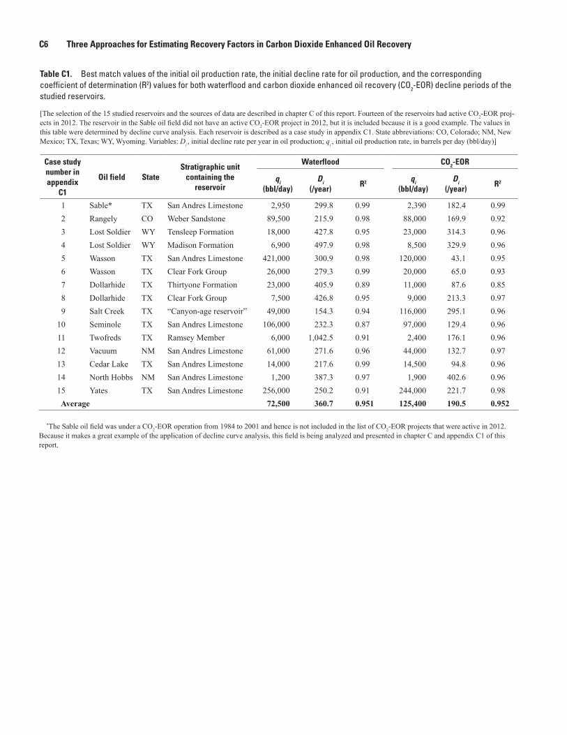
Table C1. Best match values of the initial oil production rate, the initial decline rate for oil production, and the corresponding coefficient of determination (R2) values for both waterflood and carbon dioxide enhanced oil recovery (CO2-EOR) decline periods of the studied reservoirs.

[The selection of the 15 studied reservoirs and the sources of data are described in chapter C of this report. Fourteen of the reservoirs had active CO2-EOR proj-ects in 2012. The reservoir in the Sable oil field did not have an active CO2-EOR project in 2012, but it is included because it is a good example. The values in this table were determined by decline curve analysis. Each reservoir is described as a case study in appendix C1. State abbreviations: CO, Colorado; NM, New Mexico; TX, Texas; WY, Wyoming. Variables: Di , initial decline rate per year in oil production; qi , initial oil production rate, in barrels per day (bbl/day)]

Case study number in appendix

C1

Oil field StateStratigraphic unit

containing the reservoir

Waterflood CO2-EOR

qi (bbl/day)

Di (/year)

R2 qi (bbl/day)

Di (/year)

R2

1 Sable* TX San Andres Limestone 2,950 299.8 0.99 2,390 182.4 0.992 Rangely CO Weber Sandstone 89,500 215.9 0.98 88,000 169.9 0.923 Lost Soldier WY Tensleep Formation 18,000 427.8 0.95 23,000 314.3 0.964 Lost Soldier WY Madison Formation 6,900 497.9 0.98 8,500 329.9 0.965 Wasson TX San Andres Limestone 421,000 300.9 0.98 120,000 43.1 0.956 Wasson TX Clear Fork Group 26,000 279.3 0.99 20,000 65.0 0.937 Dollarhide TX Thirtyone Formation 23,000 405.9 0.89 11,000 87.6 0.858 Dollarhide TX Clear Fork Group 7,500 426.8 0.95 9,000 213.3 0.979 Salt Creek TX “Canyon-age reservoir” 49,000 154.3 0.94 116,000 295.1 0.96

10 Seminole TX San Andres Limestone 106,000 232.3 0.87 97,000 129.4 0.9611 Twofreds TX Ramsey Member 6,000 1,042.5 0.91 2,400 176.1 0.9612 Vacuum NM San Andres Limestone 61,000 271.6 0.96 44,000 132.7 0.9713 Cedar Lake TX San Andres Limestone 14,000 217.6 0.99 14,500 94.8 0.9614 North Hobbs NM San Andres Limestone 1,200 387.3 0.97 1,900 402.6 0.9615 Yates TX San Andres Limestone 256,000 250.2 0.91 244,000 221.7 0.98Average 72,500 360.7 0.951 125,400 190.5 0.952

*The Sable oil field was under a CO2-EOR operation from 1984 to 2001 and hence is not included in the list of CO2-EOR projects that were active in 2012. Because it makes a great example of the application of decline curve analysis, this field is being analyzed and presented in chapter C and appendix C1 of this report.


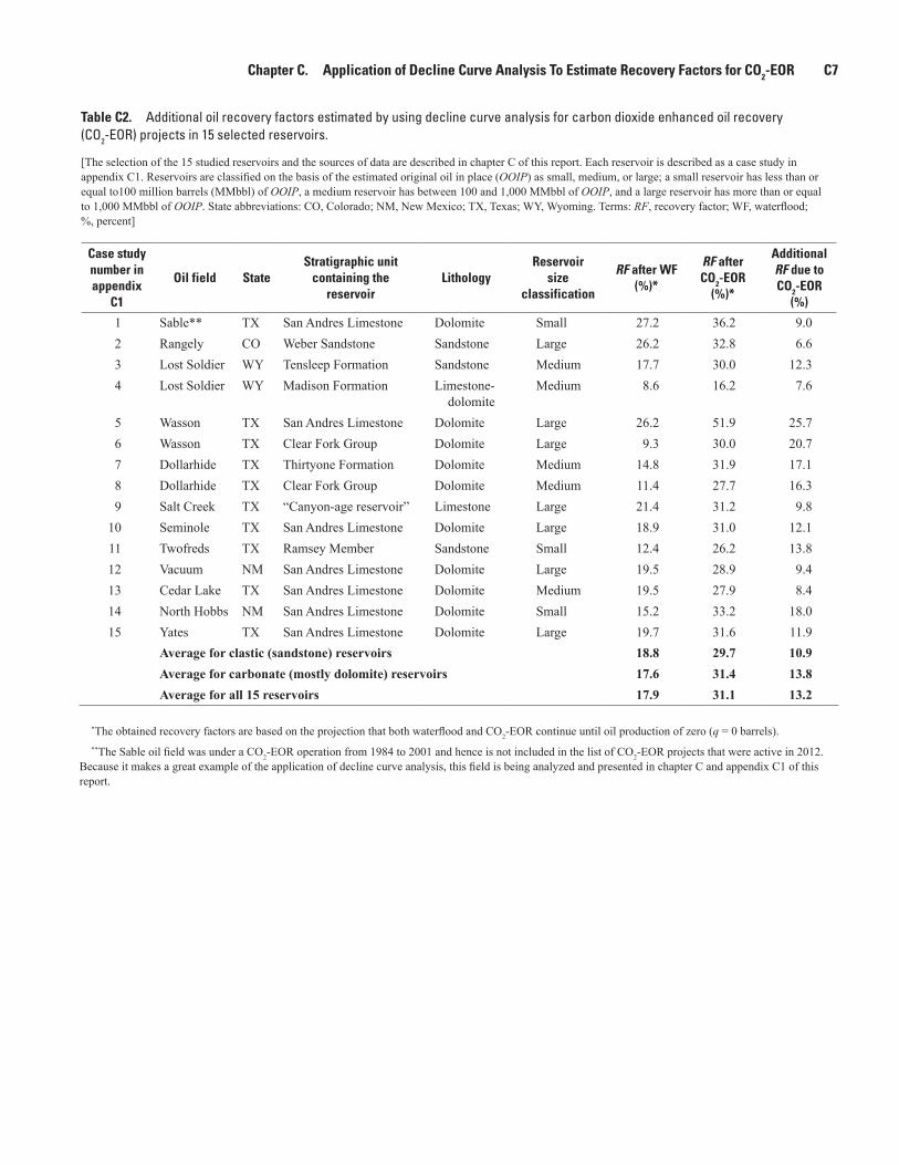
Table C2. Additional oil recovery factors estimated by using decline curve analysis for carbon dioxide enhanced oil recovery (CO2-EOR) projects in 15 selected reservoirs.

[The selection of the 15 studied reservoirs and the sources of data are described in chapter C of this report. Each reservoir is described as a case study in appendix C1. Reservoirs are classified on the basis of the estimated original oil in place (OOIP) as small, medium, or large; a small reservoir has less than or equal to100 million barrels (MMbbl) of OOIP, a medium reservoir has between 100 and 1,000 MMbbl of OOIP, and a large reservoir has more than or equal to 1,000 MMbbl of OOIP. State abbreviations: CO, Colorado; NM, New Mexico; TX, Texas; WY, Wyoming. Terms: RF, recovery factor; WF, waterflood; %, percent]

Case study number in appendix

C1

Oil field StateStratigraphic unit

containing the reservoir

LithologyReservoir

size classification

RF after WF (%)*

RF after CO2-EOR

(%)*

Additional RF due to CO2-EOR

(%)

1 Sable** TX San Andres Limestone Dolomite Small 27.2 36.2 9.02 Rangely CO Weber Sandstone Sandstone Large 26.2 32.8 6.63 Lost Soldier WY Tensleep Formation Sandstone Medium 17.7 30.0 12.34 Lost Soldier WY Madison Formation Limestone-

dolomiteMedium 8.6 16.2 7.6

5 Wasson TX San Andres Limestone Dolomite Large 26.2 51.9 25.76 Wasson TX Clear Fork Group Dolomite Large 9.3 30.0 20.77 Dollarhide TX Thirtyone Formation Dolomite Medium 14.8 31.9 17.18 Dollarhide TX Clear Fork Group Dolomite Medium 11.4 27.7 16.39 Salt Creek TX “Canyon-age reservoir” Limestone Large 21.4 31.2 9.8

10 Seminole TX San Andres Limestone Dolomite Large 18.9 31.0 12.111 Twofreds TX Ramsey Member Sandstone Small 12.4 26.2 13.812 Vacuum NM San Andres Limestone Dolomite Large 19.5 28.9 9.413 Cedar Lake TX San Andres Limestone Dolomite Medium 19.5 27.9 8.414 North Hobbs NM San Andres Limestone Dolomite Small 15.2 33.2 18.015 Yates TX San Andres Limestone Dolomite Large 19.7 31.6 11.9

Average for clastic (sandstone) reservoirs 18.8 29.7 10.9Average for carbonate (mostly dolomite) reservoirs 17.6 31.4 13.8Average for all 15 reservoirs 17.9 31.1 13.2

*The obtained recovery factors are based on the projection that both waterflood and CO2-EOR continue until oil production of zero (q = 0 barrels).**The Sable oil field was under a CO2-EOR operation from 1984 to 2001 and hence is not included in the list of CO2-EOR projects that were active in 2012.

Because it makes a great example of the application of decline curve analysis, this field is being analyzed and presented in chapter C and appendix C1 of this report.

Appendix C1. Decline Curve Analysis of Selected Reservoirs


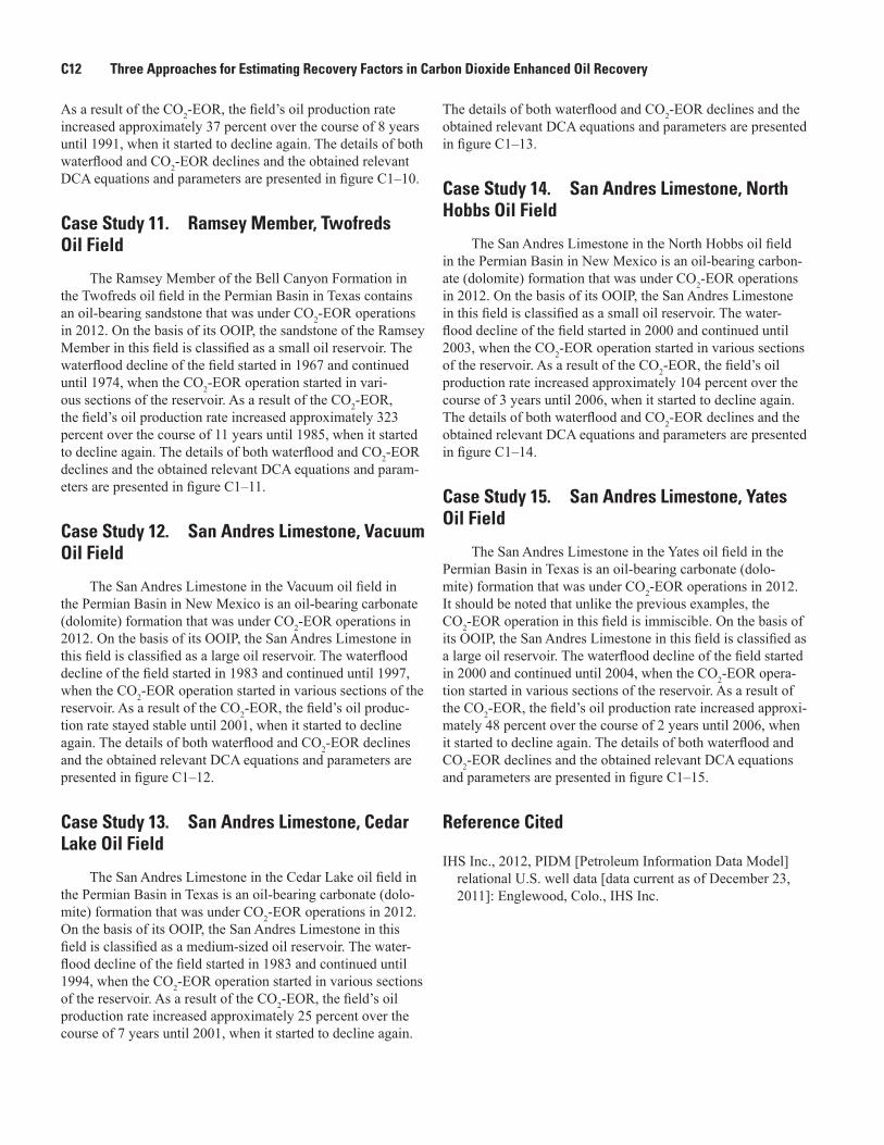
Appendix C1. Decline Curve Analysis of Selected Reservoirsboth waterflood and CO2-EOR declines and the relevant DCA equations and parameters are presented in figure C1–1.

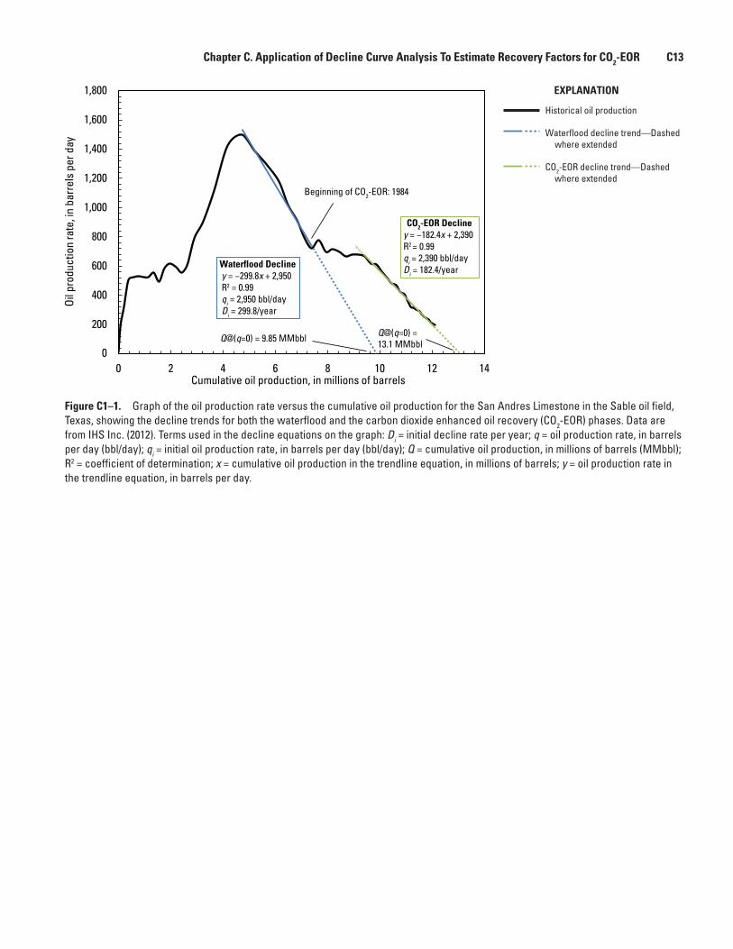
Case Study 2. Weber Sandstone, Rangely Oil Field

The Weber Sandstone in the Rangely oil field in Colo-rado is an oil-bearing sandstone formation that was under CO2-EOR operations in 2012. On the basis of its OOIP, the Weber Sandstone in this field is classified as a large oil reservoir. The waterflood decline of the field started in 1978 and continued until 1986, when the CO2-EOR operation started in various sections of the reservoir. As a result of the CO2-EOR, the field’s oil production rate increased approxi-mately 10 percent over the course of 5 years until 1991, when the decline in production started again. This reservoir was among the largest clastic reservoirs undergoing CO2-EOR in 2012. The details of both waterflood and CO2-EOR declines and the obtained relevant DCA equations and parameters are presented in figure C1–2.

Case Study 3. Tensleep Formation, Lost Soldier Oil Field

The Tensleep Formation in the Lost Soldier oil field in Wyoming is an oil-bearing sandstone formation that was under CO2-EOR operations in 2012. On the basis of its OOIP, the Tensleep Formation in this field is classified as a medium-sized oil reservoir. The waterflood decline of the field started in 1978 and continued until 1988, when the CO2-EOR opera-tion started in various sections of the reservoir. As a result of the CO2-EOR, the field’s oil production rate increased approxi-mately 300 percent over the course of 3 years until 1991, when the decline in production started again. The production profile of this reservoir shows two distinct and classical declines for both waterflood and CO2-EOR periods. The details of both waterflood and CO2-EOR declines and the obtained relevant DCA equations and parameters are presented in figure C1–3.

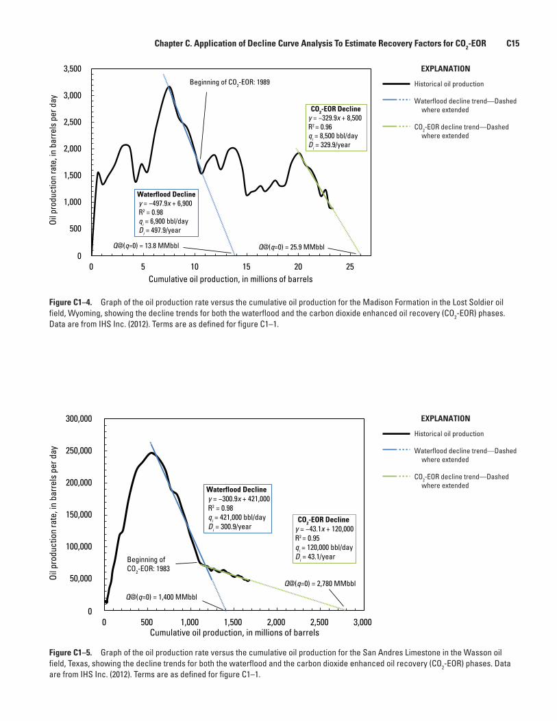
Case Study 4. Madison Formation, Lost Soldier Oil Field

The Madison Formation in the Lost Soldier oil field in Wyoming is an oil-bearing carbonate (limestone-dolomite) formation that was under CO2-EOR operations in 2012. On the basis of its OOIP, the Madison Formation in this field is clas-sified as a medium-sized oil reservoir. The waterflood decline of the field started in 1984 and continued until 1989, when the CO2-EOR operation started in various sections of the reser-voir. As a result of the CO2-EOR, the field’s oil production rate increased approximately 40 percent over the course of 16

The 15 reservoirs for case studies of decline curve analy-sis (DCA) were chosen because adequate geologic, reservoir, and production data were available for them. They all possess specific data on reservoir and fluid properties and vary signifi-cantly in terms of (1) size, as is obvious from their reported original oil in place (OOIP), (2) rock types, as they contain both clastic and carbonate reservoirs, (3) geographical loca-tions, being distributed in different basins throughout Texas, New Mexico, Wyoming, and Colorado, and (4) source of car-bon dioxide (CO2), as they use both natural and industrial CO2. Miscible carbon dioxide enhanced oil recovery (CO2-EOR) operations were used in 14 reservoirs, and an immiscible operation was used in 1 reservoir (case study 15). Fourteen of the reservoirs had active CO2-EOR projects in 2012. The reservoir in the Sable oil field (case study 1) did not have an active CO2-EOR project in 2012, but it is included because it is a good example. The 15 reservoirs all make great examples and case studies in demonstrating the applicability of DCA in predicting the behavior of decline periods for both waterflood and CO2-EOR phases.

The DCA was applied to the period of declining produc-tion of each reservoir separately, and the DCA parameters were obtained by curve fitting. The goodness of the obtained fit is presented by values for the coefficient of determina-tion, R2, which are reported separately on the graph for each reservoir analyzed (figs. C1–1 to C1–15). The closer the value of R2 is to 1, the better the quality of the fit. The obtained DCA parameters were utilized to forecast the cumulative oil produc-tion when the oil production rates were available over the life of the reservoir for both waterflood and CO2-EOR phases; for this study, the economic hydrocarbon production rate (qec) is assumed to be 0 reservoir barrels per day. This process also made it possible to estimate the reservoir’s additional oil recovery due to the CO2-EOR operation that was modeled.

It is important to note that this study does not present the technical and operational details of reservoirs described in the case studies. Nor does it provide a detailed insight into the extent of the CO2-EOR operation for each investigated project.

Case Study 1. San Andres Limestone, Sable Oil Field

The San Andres Limestone in the Sable oil field in Texas is an oil-bearing dolomite formation that was under CO2-EOR operation between 1984 and 2001. On the basis of its OOIP, the San Andres Limestone in this field is considered a relatively small oil reservoir. The production decline under waterflood started in 1976 and continued until 1984 when the CO2-EOR operation was initiated in various sections of the reservoir. As a result of the CO2-EOR, the field’s oil produc-tion rate remained stable over the course of 9 years until 1993, when the oil production began to decline again. The details of


years until 2005, when the decline in production started again. The production profile of this reservoir shows two distinct and classical declines for both waterflood and CO2-EOR periods. The details of both waterflood and CO2-EOR declines and the obtained relevant DCA equations and parameters are presented in figure C1–4.

Case Study 5. San Andres Limestone, Wasson Oil Field

The San Andres Limestone in the Wasson oil field in the Permian Basin in Texas is an oil-bearing carbonate (dolomite) formation that was under CO2-EOR operations in 2012. On the basis of its OOIP, the San Andres Limestone in this field is classified as a large oil reservoir. The waterflood decline of the field started in 1975 and continued until 1983, when the CO2-EOR operation started in various sections of the reservoir. As a result of the CO2-EOR, the field’s oil production decline rate has decreased since. The San Andres Limestone in the Wasson field is one of the largest carbonate reservoirs under-going CO2-EOR worldwide. The details of both waterflood and CO2-EOR declines and the obtained relevant DCA equa-tions and parameters are presented in figure C1–5.

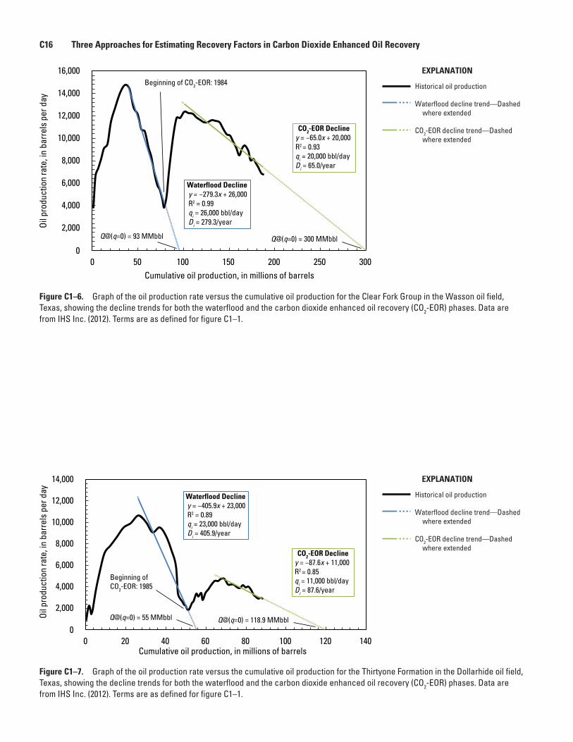
Case Study 6. Clear Fork Group, Wasson Oil Field

The Clear Fork Group in the Wasson oil field in the Permian Basin in Texas is an oil-bearing carbonate (dolomite) formation that was under CO2-EOR operations in 2012. On the basis of its OOIP, the Clear Fork Group in this field is classi-fied as a large oil reservoir. The waterflood decline of the field started in 1968 and continued until 1984, when the CO2-EOR operation started in various sections of the reservoir. As a result of the CO2-EOR, the field’s oil production rate increased approximately 93 percent over the course of 13 years until 1997, when it started to decline again. The details of both waterflood and CO2-EOR declines and the obtained relevant DCA equations and parameters are presented in figure C1–6.

Case Study 7. Thirtyone Formation, Dollarhide Oil Field

The Thirtyone Formation in the Dollarhide oil field in the Permian Basin in Texas is an oil-bearing chert and carbonate (dolomite) formation that was under CO2-EOR operations in 2012. On the basis of its OOIP, the Thirtyone Formation in this field is classified as a medium-sized oil reservoir. The water-flood decline of the field started in 1965 and continued until 1985, when the CO2-EOR operation started in various sections of the reservoir. As a result of the CO2-EOR, the field’s oil production rate increased approximately 118 percent over the course of 13 years until 1998, when it started to decline again. This reservoir is one of the best examples to demonstrate

clearly the effect of CO2-EOR on a reservoir’s oil production rate and cumulative production. The details of both waterflood and CO2-EOR declines and the obtained relevant DCA equa-tions and parameters are presented in figure C1–7.

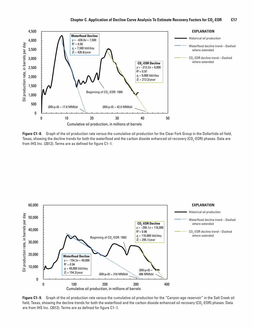
Case Study 8. Clear Fork Group, Dollarhide Oil Field

The Clear Fork Group in the Dollarhide oil field in the Permian Basin in Texas is an oil-bearing carbonate (dolomite) formation that was under CO2-EOR operations in 2012. On the basis of its OOIP, the Clear Fork Group in this field is classi-fied as a medium-sized oil reservoir. The waterflood decline of the field started in 1970 and continued until 1977. On the basis of the available production data, it is not possible to investi-gate what happened between 1977 and 1995, during which time the reservoir oil production rate stopped declining and increased slightly. This change in the oil production decline could be due to infill drilling and (or) changes in the water-flood scheme in different sections of the reservoir. In Novem-ber 1995, the CO2-EOR operation started in this reservoir. As a result of the CO2-EOR, the field’s oil production rate increased approximately 139 percent over the course of 4 years until 1999, when it started to decline again. The details of both waterflood and CO2-EOR declines and the obtained relevant DCA equations and parameters are presented in figure C1–8.

Case Study 9. “Canyon-age reservoir,” Salt Creek Oil Field

The “Canyon-age reservoir” in the Salt Creek oil field in the Permian Basin in Texas is an oil-bearing carbonate (limestone) formation that was under CO2-EOR operations in 2012. On the basis of its OOIP, the “Canyon-age reservoir” in this field is classified as a large oil reservoir. The waterflood decline of the field started in 1972 and continued until 1993, when the CO2-EOR operation started in various sections of the reservoir. As a result of the CO2-EOR, the field’s oil produc-tion rate increased approximately 38 percent over the course of 4 years until 1997, when it started to decline again. The details of both waterflood and CO2-EOR declines and the obtained relevant DCA equations and parameters are presented in figure C1–9.

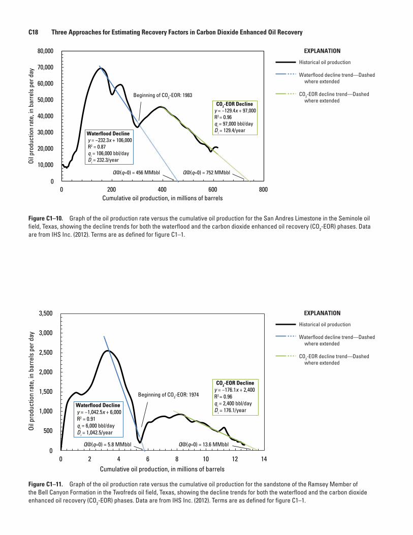
Case Study 10. San Andres Limestone, Seminole Oil Field

The San Andres Limestone in the Seminole oil field in the Permian Basin in Texas is an oil-bearing carbonate (dolomite) formation that was under CO2-EOR operations in 2012. On the basis of its OOIP, the San Andres Limestone in this field is classified as a large oil reservoir. The waterflood decline of the field started in 1977 and continued until 1983, when the CO2-EOR operation started in various sections of the reservoir.


As a result of the CO2-EOR, the field’s oil production rate increased approximately 37 percent over the course of 8 years until 1991, when it started to decline again. The details of both waterflood and CO2-EOR declines and the obtained relevant DCA equations and parameters are presented in figure C1–10.

Case Study 11. Ramsey Member, Twofreds Oil Field

The Ramsey Member of the Bell Canyon Formation in the Twofreds oil field in the Permian Basin in Texas contains an oil-bearing sandstone that was under CO2-EOR operations in 2012. On the basis of its OOIP, the sandstone of the Ramsey Member in this field is classified as a small oil reservoir. The waterflood decline of the field started in 1967 and continued until 1974, when the CO2-EOR operation started in vari-ous sections of the reservoir. As a result of the CO2-EOR, the field’s oil production rate increased approximately 323 percent over the course of 11 years until 1985, when it started to decline again. The details of both waterflood and CO2-EOR declines and the obtained relevant DCA equations and param-eters are presented in figure C1–11.

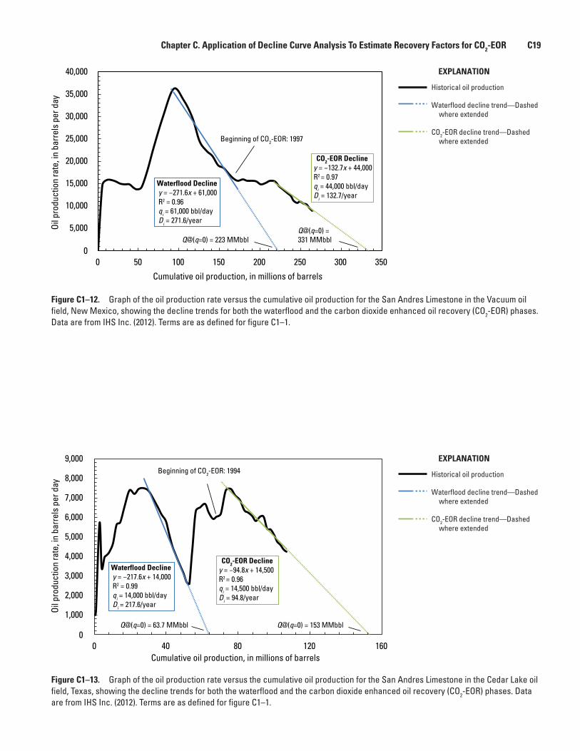
Case Study 12. San Andres Limestone, Vacuum Oil Field

The San Andres Limestone in the Vacuum oil field in the Permian Basin in New Mexico is an oil-bearing carbonate (dolomite) formation that was under CO2-EOR operations in 2012. On the basis of its OOIP, the San Andres Limestone in this field is classified as a large oil reservoir. The waterflood decline of the field started in 1983 and continued until 1997, when the CO2-EOR operation started in various sections of the reservoir. As a result of the CO2-EOR, the field’s oil produc-tion rate stayed stable until 2001, when it started to decline again. The details of both waterflood and CO2-EOR declines and the obtained relevant DCA equations and parameters are presented in figure C1–12.

Case Study 13. San Andres Limestone, Cedar Lake Oil Field

The San Andres Limestone in the Cedar Lake oil field in the Permian Basin in Texas is an oil-bearing carbonate (dolo-mite) formation that was under CO2-EOR operations in 2012. On the basis of its OOIP, the San Andres Limestone in this field is classified as a medium-sized oil reservoir. The water-flood decline of the field started in 1983 and continued until 1994, when the CO2-EOR operation started in various sections of the reservoir. As a result of the CO2-EOR, the field’s oil production rate increased approximately 25 percent over the course of 7 years until 2001, when it started to decline again.

The details of both waterflood and CO2-EOR declines and the obtained relevant DCA equations and parameters are presented in figure C1–13.

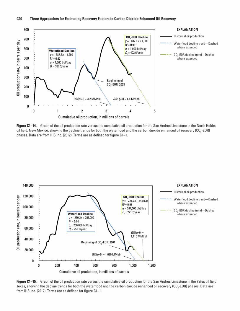
Case Study 14. San Andres Limestone, North Hobbs Oil Field

The San Andres Limestone in the North Hobbs oil field in the Permian Basin in New Mexico is an oil-bearing carbon-ate (dolomite) formation that was under CO2-EOR operations in 2012. On the basis of its OOIP, the San Andres Limestone in this field is classified as a small oil reservoir. The water-flood decline of the field started in 2000 and continued until 2003, when the CO2-EOR operation started in various sections of the reservoir. As a result of the CO2-EOR, the field’s oil production rate increased approximately 104 percent over the course of 3 years until 2006, when it started to decline again. The details of both waterflood and CO2-EOR declines and the obtained relevant DCA equations and parameters are presented in figure C1–14.

Case Study 15. San Andres Limestone, Yates Oil Field

The San Andres Limestone in the Yates oil field in the Permian Basin in Texas is an oil-bearing carbonate (dolo-mite) formation that was under CO2-EOR operations in 2012. It should be noted that unlike the previous examples, the CO2-EOR operation in this field is immiscible. On the basis of its OOIP, the San Andres Limestone in this field is classified as a large oil reservoir. The waterflood decline of the field started in 2000 and continued until 2004, when the CO2-EOR opera-tion started in various sections of the reservoir. As a result of the CO2-EOR, the field’s oil production rate increased approxi-mately 48 percent over the course of 2 years until 2006, when it started to decline again. The details of both waterflood and CO2-EOR declines and the obtained relevant DCA equations and parameters are presented in figure C1–15.

Reference Cited

IHS Inc., 2012, PIDM [Petroleum Information Data Model] relational U.S. well data [data current as of December 23, 2011]: Englewood, Colo., IHS Inc.


CO2-EOR Decliney = −182.4x + 2,390R2 = 0.99qi = 2,390 bbl/dayDi = 182.4/yearWaterflood Decline

y = −299.8x + 2,950R2 = 0.99qi = 2,950 bbl/dayDi = 299.8/year

200

400

600

800

1,000

1,200

1,400

1,600

1,800

0 2 4 6 8 10 12 14

Oil p

rodu

ctio

n ra

te, i

n ba

rrel

s pe

r day



Q@(q=0) = 9.85 MMbbl Q@(q=0) = 13.1 MMbbl

0

EXPLANATION




Figure C1–1. Graph of the oil production rate versus the cumulative oil production for the San Andres Limestone in the Sable oil field, Texas, showing the decline trends for both the waterflood and the carbon dioxide enhanced oil recovery (CO2-EOR) phases. Data are from IHS Inc. (2012). Terms used in the decline equations on the graph: Di = initial decline rate per year; q = oil production rate, in barrels per day (bbl/day); qi = initial oil production rate, in barrels per day (bbl/day); Q = cumulative oil production, in millions of barrels (MMbbl); R2 = coefficient of determination; x = cumulative oil production in the trendline equation, in millions of barrels; y = oil production rate in the trendline equation, in barrels per day.


10,000

20,000

30,000

40,000

50,000

60,000

70,000

0 100 200 300 400 500

Oil p

rodu

ctio

n ra

te, i

n ba

rrel

s pe

r day


0


Waterflood Decliney = −215.9x + 89,500R2 = 0.98qi = 89,500 bbl/dayDi = 215.9/year

CO2-EOR Decliney = −169.9x + 88,000R2 = 0.92qi = 88,000 bbl/dayDi = 169.9/year

Q@(q=0) = 414 MMbbl Q@(q=0) = 519 MMbbl

EXPLANATION




Figure C1–2. Graph of the oil production rate versus the cumulative oil production for the Weber Sandstone in the Rangely oil field, Colorado, showing the decline trends for both the waterflood and the carbon dioxide enhanced oil recovery (CO2-EOR) phases. Data are from IHS Inc. (2012). Terms are as defined for figure C1–1. For completeness, this figure is included in the appendix even though it is also shown as text-figure C2.

2,000

4,000

6,000

8,000

10,000

12,000

14,000

0 10 20 30 40 50 60 70 80

Oil p

rodu

ctio

n ra

te, i

n ba

rrel

s pe

r day


0




Q@(q=0) = 42.6 MMbblQ@(q=0) = 71.9 MMbbl

EXPLANATION




Figure C1–3. Graph of the oil production rate versus the cumulative oil production for the Tensleep Formation in the Lost Soldier oil field, Wyoming, showing the decline trends for both the waterflood and the carbon dioxide enhanced oil recovery (CO2-EOR) phases. Data are from IHS Inc. (2012). Terms are as defined for figure C1–1.


500

1,000

1,500

2,000

2,500

3,000

3,500

0 5 10 15 20 250

Oil p

rodu

ctio

n ra

te, i

n ba

rrel

s pe

r day




Q@(q=0) = 13.8 MMbbl


Q@(q=0) = 25.9 MMbbl

EXPLANATION




Figure C1–4. Graph of the oil production rate versus the cumulative oil production for the Madison Formation in the Lost Soldier oil field, Wyoming, showing the decline trends for both the waterflood and the carbon dioxide enhanced oil recovery (CO2-EOR) phases. Data are from IHS Inc. (2012). Terms are as defined for figure C1–1.

50,000

100,000

150,000

200,000

250,000

300,000

0 500 1,000 1,500 2,000 2,500 3,0000

Oil p

rodu

ctio

n ra

te, i

n ba

rrel

s pe

r day


Q@(q=0) = 1,400 MMbbl


Q@(q=0) = 2,780 MMbbl



EXPLANATION




Figure C1–5. Graph of the oil production rate versus the cumulative oil production for the San Andres Limestone in the Wasson oil field, Texas, showing the decline trends for both the waterflood and the carbon dioxide enhanced oil recovery (CO2-EOR) phases. Data are from IHS Inc. (2012). Terms are as defined for figure C1–1.


2,000

4,000

6,000

8,000

10,000

12,000

14,000

16,000

0 50 100 150 200 250 3000

Oil p

rodu

ctio

n ra

te, i

n ba

rrel

s pe

r day



Q@(q=0) = 93 MMbbl Q@(q=0) = 300 MMbbl



EXPLANATION




Figure C1–6. Graph of the oil production rate versus the cumulative oil production for the Clear Fork Group in the Wasson oil field, Texas, showing the decline trends for both the waterflood and the carbon dioxide enhanced oil recovery (CO2-EOR) phases. Data are from IHS Inc. (2012). Terms are as defined for figure C1–1.

2,000

4,000

6,000

8,000

10,000

12,000

14,000

0 20 40 60 80 100 120 1400

Oil p

rodu

ctio

n ra

te, i

n ba

rrel

s pe

r day



Q@(q=0) = 55 MMbbl Q@(q=0) = 118.9 MMbbl



EXPLANATION




Figure C1–7. Graph of the oil production rate versus the cumulative oil production for the Thirtyone Formation in the Dollarhide oil field, Texas, showing the decline trends for both the waterflood and the carbon dioxide enhanced oil recovery (CO2-EOR) phases. Data are from IHS Inc. (2012). Terms are as defined for figure C1–1.


500

1,000

1,500

2,000

2,500

3,000

3,500

4,000

4,500

0 10 20 30 40 500

Oil p

rodu

ctio

n ra

te, i

n ba

rrel

s pe

r day


Q@(q=0) = 17.8 MMbbl Q@(q=0) = 42.0 MMbbl




EXPLANATION




Figure C1–8. Graph of the oil production rate versus the cumulative oil production for the Clear Fork Group in the Dollarhide oil field, Texas, showing the decline trends for both the waterflood and the carbon dioxide enhanced oil recovery (CO2-EOR) phases. Data are from IHS Inc. (2012). Terms are as defined for figure C1–1.

10,000

20,000

30,000

40,000

50,000

60,000

0 100 200 300 4000

Oil p

rodu

ctio

n ra

te, i

n ba

rrel

s pe

r day



Q@(q=0) = 316 MMbblQ@(q=0) = 386 MMbbl



EXPLANATION




Figure C1–9. Graph of the oil production rate versus the cumulative oil production for the “Canyon-age reservoir” in the Salt Creek oil field, Texas, showing the decline trends for both the waterflood and the carbon dioxide enhanced oil recovery (CO2-EOR) phases. Data are from IHS Inc. (2012). Terms are as defined for figure C1–1.


10,000

20,000

30,000

40,000

50,000

60,000

70,000

80,000

0 200 400 600 8000

Oil p

rodu

ctio

n ra

te, i

n ba

rrel

s pe

r day



Q@(q=0) = 456 MMbbl Q@(q=0) = 752 MMbbl



EXPLANATION




Figure C1–10. Graph of the oil production rate versus the cumulative oil production for the San Andres Limestone in the Seminole oil field, Texas, showing the decline trends for both the waterflood and the carbon dioxide enhanced oil recovery (CO2-EOR) phases. Data are from IHS Inc. (2012). Terms are as defined for figure C1–1.

500

1,000

1,500

2,000

2,500

3,000

3,500

0 2 4 6 8 10 12 140

Oil p

rodu

ctio

n ra

te, i

n ba

rrel

s pe

r day



Q@(q=0) = 5.8 MMbbl Q@(q=0) = 13.6 MMbbl

Waterflood Decliney = −1,042.5x + 6,000R2 = 0.91qi = 6,000 bbl/dayDi = 1,042.5/year


EXPLANATION




Figure C1–11. Graph of the oil production rate versus the cumulative oil production for the sandstone of the Ramsey Member of the Bell Canyon Formation in the Twofreds oil field, Texas, showing the decline trends for both the waterflood and the carbon dioxide enhanced oil recovery (CO2-EOR) phases. Data are from IHS Inc. (2012). Terms are as defined for figure C1–1.


5,000

10,000

15,000

20,000

25,000

30,000

35,000

40,000

0 50 100 150 200 250 300 3500

Oil p

rodu

ctio

n ra

te, i

n ba

rrel

s pe

r day



Q@(q=0) = 223 MMbblQ@(q=0) = 331 MMbbl



EXPLANATION




Figure C1–12. Graph of the oil production rate versus the cumulative oil production for the San Andres Limestone in the Vacuum oil field, New Mexico, showing the decline trends for both the waterflood and the carbon dioxide enhanced oil recovery (CO2-EOR) phases. Data are from IHS Inc. (2012). Terms are as defined for figure C1–1.

1,000

2,000

3,000

4,000

5,000

6,000

7,000

8,000

9,000

0 40 80 120 1600

Oil p

rodu

ctio

n ra

te, i

n ba

rrel

s pe

r day



Q@(q=0) = 63.7 MMbbl Q@(q=0) = 153 MMbbl



EXPLANATION




Figure C1–13. Graph of the oil production rate versus the cumulative oil production for the San Andres Limestone in the Cedar Lake oil field, Texas, showing the decline trends for both the waterflood and the carbon dioxide enhanced oil recovery (CO2-EOR) phases. Data are from IHS Inc. (2012). Terms are as defined for figure C1–1.


100

200

300

400

500

600

700

800

0 1 2 3 4 50

Oil p

rodu

ctio

n ra

te, i

n ba

rrel

s pe

r day



Q@(q=0) = 3.2 MMbbl Q@(q=0) = 4.8 MMbbl



EXPLANATION




Figure C1–14. Graph of the oil production rate versus the cumulative oil production for the San Andres Limestone in the North Hobbs oil field, New Mexico, showing the decline trends for both the waterflood and the carbon dioxide enhanced oil recovery (CO2-EOR) phases. Data are from IHS Inc. (2012). Terms are as defined for figure C1–1.

20,000

40,000

60,000

80,000

100,000

120,000

140,000

0 200 400 600 800 1,000 1,2000

Oil p

rodu

ctio

n ra

te, i

n ba

rrel

s pe

r day



Q@(q=0) = 1,030 MMbbl

Q@(q=0) = 1,110 MMbbl



EXPLANATION




Figure C1–15. Graph of the oil production rate versus the cumulative oil production for the San Andres Limestone in the Yates oil field, Texas, showing the decline trends for both the waterflood and the carbon dioxide enhanced oil recovery (CO2-EOR) phases. Data are from IHS Inc. (2012). Terms are as defined for figure C1–1.

Documents

Application of Decline Curve Analysis To Estimate Recovery ... · Application of Decline Curve Analysis To Estimate Recovery Factors for Carbon Dioxide Enhanced Oil Recovery By Hossein