Application of field geophysics in geomorphology: Advances

Available online at www.sciencedirect.com

(2008) 55–73www.elsevier.com/locate/geomorph

Geomorphology 93

Application of field geophysics in geomorphology: Advances andlimitations exemplified by case studies

Lothar Schrott a,⁎, Oliver Sass b

a Department of Geography and Geology, University of Salzburg, Hellbrunnerstr. 34, A-5020 Salzburg, Austriab Department of Geography, University of Augsburg, Universitätsstr. 10, D-86135 Augsburg, Germany

Received 30 December 2005; accepted 27 December 2006Available online 10 May 2007

Abstract

During the last decade, the use of geophysical techniques has becomepopular inmany geomorphological studies.However, the correcthandling of geophysical instruments and the subsequent processing of the data they yield are difficult tasks. Furthermore, the descriptionand interpretation of geomorphological settings to which they apply can significantly influence the data gathering and subsequentmodelling procedure (e.g. achieving a maximum depth of 30 m requires a certain profile length and geophone spacing or a particularfrequency of antenna). For more than three decades geophysical techniques have been successfully applied, for example, in permafroststudies. However, in many cases complex or more heterogeneous subsurface structures could not be adequately interpreted due to limitedcomputer facilities and time consuming calculations. As a result of recent technical improvements, geophysical techniques have beenapplied to a wider spectrum of geomorphological and geological settings. This paper aims to present some examples of geomorphologicalstudies that demonstrate the powerful integration of geophysical techniques and highlight some of the limitations of these techniques. Afocus has been given to the three most frequently used techniques in geomorphology to date, namely ground-penetrating radar, seismicrefraction and DC resistivity. Promising applications are reported for a broad range of landforms and environments, such as talus slopes,block fields, landslides, complex valley fill deposits, karst and loess covered landforms. A qualitative assessment highlights suitablelandforms and environments. The techniques can help to answer yet unsolved questions in geomorphological research regarding forexample sediment thickness and internal structures. However, based on case studies it can be shown that the use of a single geophysicaltechnique or a single interpretation tool is not recommended for many geomorphological surface and subsurface conditions as this maylead to significant errors in interpretation. Because of changing physical properties of the subsurfacematerial (e.g. sediment,water content)in many cases only a combination of two or sometimes even three geophysical methods gives sufficient insight to avoid seriousmisinterpretation. A “good practice guide” has been framed that provides recommendations to enable the successful application of threeimportant geophysical methods in geomorphology and to help users avoid making serious mistakes.© 2007 Elsevier B.V. All rights reserved.

Keywords: Ground-penetrating radar; DC resistivity; Seismic refraction; Landforms; Internal structure

⁎ Corresponding author.E-mail addresses: [email protected] (L. Schrott),

[email protected] (O. Sass).

0169-555X/$ - see front matter © 2007 Elsevier B.V. All rights reserved.doi:10.1016/j.geomorph.2006.12.024

1. Introduction

Recently, the use of geophysical techniques hasbecome increasingly important in many geomorpholog-ical studies. Without the application of geophysics ourknowledge about subsurface structures, especially over

mailto:[email protected]

mailto:[email protected]

http://dx.doi.org/10.1016/j.geomorph.2006.12.024

56 L. Schrott, O. Sass / Geomorphology 93 (2008) 55–73

larger areas, remains extremely limited. During the lastdecade the use of geophysical techniques has become anew and exciting tool for many geomorphologists. Onereason for the increasing interest in geophysical fieldmethods is certainly related to technical innovations asincreased computer power and the availability of light-weight equipment allows for relatively user-friendly,efficient and non-destructive data gathering.However, thecorrect handling of the geophysical instruments andsubsequent data processing are still difficult tasks and themethods often require advanced mathematical treatmentfor interpretation. It should be pointed out that withoutclose collaboration between geomorphologists and geo-physicists the accurate and effective use of geophysicaltechniques and their geophysical and geomorphologicalinterpretation are often very limited. In addition, thecorrect description and interpretation of geomorpholog-ical settings and thus, the choice of adequate andmeaningful field sites are not an easy task.

Inmost studies and textbooks, interdisciplinary aspectscombining geophysics and geomorphology are poorlyaddressed. Many textbooks, in their description ofgeophysical surveying applications, focus on the explo-ration for fossil fuels and mineral deposits, undergroundwater supplies, engineering site and archaeologicalinvestigation (e.g. Reynolds, 1997; Kearey et al., 2002).Although several potential applications for geophysicalmethods exist, many of them have not yet been fullyintegrated into geomorphological research. The mostcommon geophysical applications are currently focusingon permafrostmapping, sediment thickness determinationof talus slopes, block fields, alluvial fans and, increas-ingly, on the depth and internal structures of landslides(Hecht, 2000; Tavkhelidse et al., 2000; Hauck, 2001;Hoffmann and Schrott, 2002; Hauck and Vonder Mühll,2003; Israil and Pachauri, 2003; Kneisel and Hauck,2003; Schrott et al., 2003; Bichler et al., 2004; Sass et al.,2007-this issue). Other landforms such as karst and colluviaare comparatively rarely investigated (Hecht, 2003).Currently, the most common geophysical methods ingeomorphological research are ground-penetrating radar,DC resistivity, and seismic refraction (Gilbert, 1999). Thus,the paper focuses on typical applications of these methods.

Each geophysical technique is based on the interpre-tation of contrasts in specific physical properties of thesubsurface (e.g. dielectric constant, electrical conductiv-ity, density). The type of physical property to which aparticular geophysical method responds determines andlimits the range of applications. As non-geophysicistscannot generally be aware of all limitations and pitfalls,there is a need to develop a set of the most suitable recipescombining geophysical methods. These methods can then

be adjusted to particular environmental conditions andlandforms. Studies that compare the application of variousinterpretation tools and discuss the combined/compositeapplications of geophysical field methods for a particularlandform are still rare (Schrott et al., 2000; Schwambornet al., 2002; Otto and Sass, 2006; Sass, 2006a,b).

Thus, the objectives of the present paper are:

(i) to show and assess the advances and limitations ofdifferent geophysical methods with the focus onapplied geomorphological research;

(ii) to demonstrate the application of these methods indifferent natural environments and for distinctivelandform types, and

(iii) to illustrate the advantages of combined andcomposite techniques leading to a set of recom-mendations for the application of field geophysicsin geomorphology.

As the paper focuses on the potential application ofthree geophysical methods in different environments,the site descriptions have been reduced to a necessaryminimum.

2. Ground-penetrating radar (GPR)

2.1. Principle and geomorphic context

Ground-penetrating radar is a technique that uses high-frequency electromagnetic waves to acquire informationon subsurface composition. The electromagnetic pulse isemitted from a transmitter antenna and propagatesthrough the subsurface at a velocity determined by thedielectric properties of the subsurfacematerials. The pulseis reflected by inhomogeneities and layer boundaries andis received by a second antenna after a measured traveltime. In order to calculate depth,wide-angle reflection andrefraction (WARR) or common mid-point (CMP) mea-surements have to be performed. These signal travel timemeasurements are made with a stepwise increase in thedistance between the two antennas. From the distance/travel time diagram, the propagation velocity of the radarwaves in the subsurface can be derived.

The common mode of GPR data collection is fixed-offset reflection profiling (Jol and Bristow, 2003). In thisstep-like procedure, the antennas are moved along aprofile line and the measurement is repeated at discreteintervals resulting in a 2-D image of the subsurface. Thepossible working frequencies can range from 10 MHz to1 GHz depending upon the aim of the investigation.Higher frequencies allow higher spatial resolution of theground information, but lead to a lower penetration depth.



57L. Schrott, O. Sass / Geomorphology 93 (2008) 55–73

This has important implications in geomorphologicalapplications. Knowledge about the geomorphologicalcontext (expected maximum depth and grain-size com-position of a sediment body) is essential for choosing theappropriate frequencies. A comprehensive “good practiceguide” for the application ofGPR in sediments is providedby Jol and Bristow (2003).

The maximum depth of investigation depends mainlyupon the dielectric constant (ε) and the electricalconductivity (σ) of the subsurface. A higher groundwater and/or clay content (high ε, high σ) leads to astronger attenuation and, therefore, a markedly reducedpenetration depth. However, very pure groundwatersthat have a low conductivity (e.g. glacial meltwater,bogs) are characterized by relatively low levels of GPRsignal loss. Again, geomorphological expertise aboutpossible water and clay layers can help to avoiddisappointing measurements. On dry and electrically

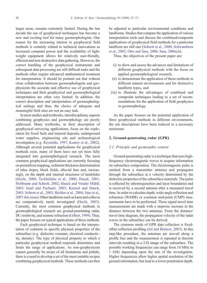
Table 1Comparison of common field geophysical methods in geomorphology; exam

Geophysical method Geomorphological application

Ground-penetratingradar (GPR)

▶Delineation of the boundaries of massive ice inrock glaciers, moraines and other periglacialphenomena▶Determining the thickness of a permafrost layer

▶Active layer thickness▶Glacial ice thickness

▶Delineation of aquifers▶Fracture mapping within massive bedrock▶Mapping of internal structures in sedimentstorage types (e.g. talus slopes, rock glaciers)

2-D DC resistivitysounding, 2-D DCresistivity profiling

▶Determining sediment thickness, internaldifferentiation and groundwater▶Depth and extension of landslide bodies

▶Detection of massive ice or permafrost in rockglaciers, moraines and other periglacial phenomena

▶Ice thickness

▶Determining the altitudinal permafrost limit

▶Moisture distribution in rock walls▶Seasonal variation in fluid content

Seismic refraction (2-Dsounding,tomography)

▶Sediment thickness (talus, alluvial fans, etc.)

▶Detection of massive ice in rock glaciers,moraines and other periglacial phenomena▶Differentiation between ice, air and special rocktypes▶Mapping active layer thickness

high-resistive debris, a penetration of between 30 and60 m can be achieved (e.g. Smith and Jol, 1995). Sandysediments are also favourable for GPR measurements atdepths of between 15 and 30 m. Due to the strongattenuation in materials that have a high electricalconductivity the penetration depth in wet, silty and/orclayey sediments diminishes rapidly to, for example, lessthan 5 m in silt (Doolittle and Collins, 1995); in clayeysoil the application of GPRmay be altogether impossible(see Table 1). This is, however, only a very rough guide,because the penetration depth depends upon the deviceand antenna frequency used. The vertical resolution ofGPR data is a function of frequency and propagationvelocity.With higher velocities, resolution decreases andvice versa. As a rule of thumb, in the medium velocityrange (0.1 m/ns) the resolution is approximately 1 musing 25 MHz antennae, 0.25 m using 100 MHz and2.5 cm using 1 GHz.

ples of applications and some technical considerations and advice

Technical considerations and practical advice

▶Small penetration depth in case of conductive near-surface layers

▶Less successful in, for example, wooded terrain with many surfacereflectors and in electrically conductive sediments (e.g. clay-rich)▶Experience in data processing and interpretation is needed▶Correlate radar data with geomorphic/geologic control and siteobservations such as exposures or borehole logs

▶Obtaining good electrical contact between electrodes and ground isessential▶Blocky and dry material is very problematic due to poor electrodecoupling▶Experience in data inversion is needed for data processing. A prioriinformation influences (improves) significantly your iterativemodelling▶Differentiation between ice, air and special rock types cansometimes be difficult▶Correlate resistivity data with geomorphic/geologic control and siteobservations such as exposures or borehole logs

▶Number of geophones should be at least 12, with shots at everyother receiver location▶Sledge hammer as source is sufficient for most shallowapplications (b30 m)▶Experience in data processing and inversion is needed for datainterpretation▶Correlate seismic data with geomorphic/geologic control and siteobservations such as exposures or borehole logs


2.2. Advantages and disadvantages of GPR

Evenwhen low-frequency 25 and 50MHz antennas areused, GPR still provides a better spatial resolution thanstandard geophysical techniques. The survey speed even inrough terrain is relatively high and several hundred metresper day are possible. Steep and rocky slopes limit theprogress of the survey, because low-frequency antennashave large geometrical dimensions and are difficult tohandle. Recently developed, so-called, Rough TerrainAntennas (RTAs) may facilitate data gathering, however,conventional antennas are still necessary for CMPmeasurements or small object detection.

The available antenna frequencies allow for a broadvariety of possible applications. However, the extremelyvariable penetration depth requires careful assessment ofthe subsurface parameters in the study area in order tominimize the risk of error. The electrical conductivity ofthe soil provides a rough indicator of potential targetdepth. From the authors' experience, the use of GPR isnot promising if the soil resistivity is lower than ca. 50–100 Ωm.

The application of GPR is subject to further restric-tions. As the reflectivity at a layer boundary is determinedby the contrast in the dielectrical properties of thesubsurface units, no distinct reflection is found whenthis contrast is low. Small-scale spatial differences inwater content and/or grain-size composition may yieldstronger reflections than the target of the investigation(e.g. the bedrock surface). This problemmay be overcomeby using the radar facies of the sediments for interpreta-tion. Different sediment units and bedrock yield typicalreflection patterns that can be derived from, for example,reference profiles. The reconnaissance of these patternssignificantly facilitates the interpretation of the radargram.

A portion of the energy transmitted by an unshieldedantenna is emitted into the air and may be reflected byfeatures above the surface. These air wave reflectionscannot always be unequivocally distinguished fromground information and may severely affect the dataquality. This makes the application of GPR particularlydifficult in wooded terrain where, depending on thefrequency used, each tree may act as a single reflector,leading to very noisy or altogether useless data. Althoughthe effect of air wave reflections may be reduced usingsophisticated filter algorithms (e.g. Van der Kruk andSlob, 2004), measuring in forested areas is not advisable.The use of shielded antennas is only possible for higherfrequencies (N100 MHz). Taking into consideration themajor restrictions arising from “clayey or silty subsur-face” and “wooded terrain” it is clear that GPR shows itspotential particularly in arctic or alpine areas above the

tree-line and where there is limited soil development.However, shallow subsurface investigations are alsopossible in fluvial deposits and even in peat, when theelectrical conductivity of the groundwater is low.

2.3. Examples of application

There is a broad range of successful applications ofGPR in geomorphological studies. These include thedetection of buried structures, assessment of internalsediment structures and estimation of depth to bedrock.Various types of sediments have been investigated forgeomorphological purposes (Bristow et al., 2000).

The internal structures of floodplain deposits anddeltaic sediments have been visualized by, for example,Leclerc and Hickin (1997), Jol (1996) and Büker et al.(1996). Buried fluvial channels have been detected byRoberts et al. (1997) and Loope et al. (2004). The mostfrequently used antenna frequency for comparative studiesis 100MHz. The penetration depth is dependant upon clayand water content, but usually ranges from 10 to 20 m.

Loose sediments in arctic and alpine areas have alsobeen the subject of GPR measurements. Lønne andLauritsen (1996) and Overgaard and Jakobsen (2001)have investigated internal deformation structures of push-moraines and Berthling et al. (2000) clearly detectedinternal structures as well as the bedrock base of rockglaciers. The working groups used 50 and 100 MHzantennas and achieved a penetration depth of up to 30 m.Sass and Wollny (2001) and Sass (2006a) achieved apenetration depth of up to 50 m on talus slopes using25 MHz antennas. They found surface-parallel structuresin the debris body and evidence formorainematerial at thebase of the talus. Studies of sediment structures have alsofrequently been carried out in bogs. Völkel et al. (2001)investigated the subsurface structure of buried periglacialslope deposits, while e.g.Holden et al. (2002) determinedthe position and depth of subsurface piping.

The application of GPR on landslides has repeatedlybeen tested but with limited success. Wollny (1999)investigated the near-surface moisture distribution at 10landslide areas and gained valuable information fromonlythree sites. Bruno and Mariller (2000) and Wetzel et al.(2006) used GPR for detecting the vertical extension oflandslides but did not reach the slip surface even with theuse of low-frequency antennas. However, internal slidestructures such as rotational features can be mapped whenthe slide surface is comparatively dry (e.g. Sass et al. (thisissue) in displaced limestone blocks). Bichler et al. (2004)obtained very good results, distinguishing seven differentfacies of loose sediments. PerformingGPRmeasurementsat landslide sites is only worthwhile when comparatively


coarse and dry deposits (debris, displaced blocks)superimpose the silty or clayey material of the slipsurface. However, detailed assessment of the near-surfacepropagation velocity allows a rather accurate estimate ofthe soil moisture content (Topp et al., 1980) which is ofinterest for landslide investigation and many moregeomorphological questions.

Another possible field of application is the investiga-tion of permafrost features. The active layer thickness hasbeen determined, for example, byArcone et al. (1998) andHinkel et al. (2001). Moorman et al. (2003) providedinstructive pictures of typical reflection patterns in frozenand unfrozen ground. Although the presence or non-presence of permafrost is more difficult to establish withGPR than electrical resistivity techniques, GPR issuperior in detecting spatially confined structures suchas ice wedges (Hinkel et al., 2001). The thickness and theinternal structure of glacier ice (unfrozen water content,cavities) have also been the target of many GPRinvestigations (e.g. Moorman and Michel, 2000).

The investigation of quasi point-shaped or linearburied structures in high resolution is the aim of manystudies in the relatively new field of geo-archaeologythat is closely related to geomorphology (Baker et al.,1997; Fuchs and Zöller, 2006). Leckebusch (2003) hasprovided a detailed description of the GPR method forarchaeological purposes with numerous examples. Theworking frequencies for these applications are usuallyrather high (=200 MHz); the target depth is usuallybetween 1 and 5 m.

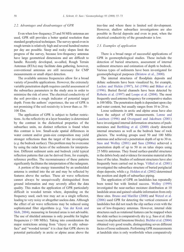
Fig. 1. Investigation of a buried Roman road using 200 MHz GPR profiles. Fidependant gain function. Above: cross profile, below: longitudinal profile. Tet al., 2004).

2.3.1. Case study: localization of buried structuresThe aim of this GPR application was to locate a

Roman road buried under 1.5 to 3 m of peat and fluvialsediments in the Murnauer Moos, Upper Bavaria (Sasset al., 2004). This example primarily highlights thepotential for archaeological studies (Fuchs and Hruska,1996). However, from a geomorphological perspectivethe Roman road can be used as a time marker for theevolution of the overlaying peat and interbedded clay-rich sediments. The road had been examined at anarchaeological excavation nearby. Thus, the structure ofthe road (logs lying on a gravel layer) was known. Theobjective of the measurements was the quick localiza-tion in the surroundings of the excavation.

As a result of the high water content of the peat, thepropagation velocity derived fromWARR measurementswas very low (0.45 m/ns). However, because of the lowmineralization of the bog water the penetration depthusing 200 MHz antennae was up to 5 m. The road wasquickly and clearly located in a number of cross profiles(Fig. 1). Thus, the measurements provided valuableinformation on the straight-line structure. The cross-profile presented (Fig. 1a) shows the radar reflection ofthe Roman road at a profile distance of between 3 and 7m.The shallow depression in the middle of the road (asobserved at the excavation site), caused by the weight ofthe vehicles, can be clearly recognized. The longitudinalprofile (Fig. 1b) illustrates the linear structure of the road.The main reflection is caused by the artificial gravel layerwhich obviously shows a distinct dielectrical contrast to

lters applied: DC-shift removal, bandpass frequency filter and runtime-he road is recognizable from typical reflection patterns (see text) (Sass


the surrounding peat. The V-shaped structures below(e.g. at profile distances of between 10 and 14 and be-tween 80 and 100 ns) are the hyperbolic reflection patternsof singular logs lying at right angles to the course ofthe road. From this typical pattern the road can be un-equivocally distinguished from geological reflectors.

In a series of cross profiles, the road was located evenin positions where borings failed to detect the structure,probably due to the advanced rotting of the logs.However, alluvial layers near the surface considerablyreduced the penetration depth due to high attenuation inthe clay. In the vicinity of some shallow alluvial cones,the penetration depth was reduced to less then 1 mwhich made the detection of any structures impossible.

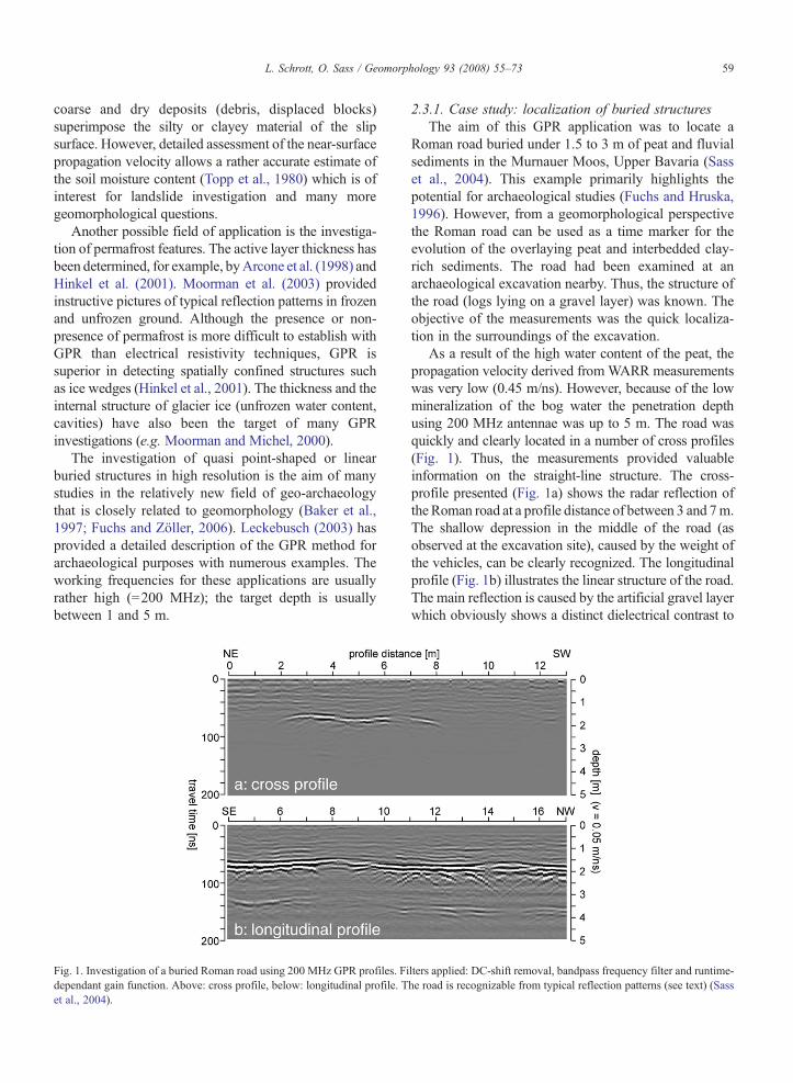
2.3.2. Case study: talus sediment thicknessFig. 2 shows the 50MHz longitudinal section of a talus

slope in the Kühtai area (Central Alps, Austria) at anelevation of between 2400 and 2600 m. The profilestretched from a moraine ridge at the foot of the talusupwards (inclined approx. 30°) to the gneiss/mica-schistrockwall (inclined at 55 to 60°). In the upslope parts of theprofile (approximately 70 to 130 m), the debris is ratherfine-grained (5 to 20 cm) and gradually gets coarsertowards the base of the slope, where boulder-sized clastsprevail.

The bedrock surface is recognizable as a distinctreflector (highlighted by the thick dashed line) revealing ashallow basin (see Fig. 2). The part of the talus body closeto the rockwall (between 60 and 110 m) is characterizedby surface-parallel, slightly undulated and partly over-lapping reflection patterns probably indicating stackedsediment layers. No comparable layers can be observednear the foot of the talus (0–60 m). This points to fluvialdistribution that is restricted to the vicinity of themoderately steep rock face. The maximum thickness ofthe debris is 12m in themiddle of the profile. In the deepersubsurface, thin lines are visible which are slantingdiagonally to the left. Considering the inclination of the

Fig. 2. 50 MHz radargram of a talus slope in the Sellrain region, Austria. Theremoval, bandpass frequency filter and runtime-dependant gain function.

profile, these lines represent reflectors dipping at an angleof between 60 to 70° to the south (left side). This agreeswith the dipping of the gneiss–micaschist layers of theadjacent rockwall. The occurrence of airborne (rockwall)reflections is improbable because of the position andangle of the reflectors, together with the low inclination ofthe rockwall above.

3. 1-D and 2-D DC resistivity


Geoelectrical sounding provides a one-dimensionalvertical profile of the electrical resistivity distributionwithdepth. Resistivity measurements are conducted byapplying a constant current into the ground through two“current electrodes” and measuring the resulting voltagedifferences at two “potential electrodes”. From the currentand voltage values, an apparent resistivity value iscalculated. 1-D surveys use only four electrodes.Generally, the two potential electrodes remain in positionin the middle of the profile, while the current electrodesmove stepwise to both sides (Schlumberger array). Thewider the electrodes are apart, the deeper the electricalfield penetrates into the ground. Thus, a depth profileunder the approximate middle of the section is created.This array has been widely used in geomorphic research(Etzelmüller et al., 2003). 2-D arrays represent a furtherdevelopment of the 1-D technique, using 50 or moreelectrodes at a time. Amicro-controller unit automaticallyswitches between numerous electrode configurations,thus creating a 2-D pseudosection of the subsurface. Theinversion of the gathered data using sophisticatedcomputer programs produces a 2-D section of thesubsurface resistivity. The Res2Dinv-software providedby Loke and Barker (1995) is the most commonly used ingeosciences. The principle of operation is based on astepwise iteration process which tries to minimize thedeviation between the measured apparent resistivity and

inclination of the slope is approximately 30°. Filters applied: DC-shift


the simulated apparent resistivity values calculated from asubsurface model. The 2-D section can also be conductedin a Schlumberger array, which provides particularly goodresolution for lateral inhomogeneities. The Wenner arrayshows a good signal–noise ratio and is favourable for thedetection of horizontal layers, while the Dipole–Dipolearray is favourable for the delimitation of spatiallyconfined objects in the shallow subsurface. For acomprehensive description of these configurations werefer to geophysical textbooks (Milsom, 1996; Reynolds,1997; Kearey et al., 2002).

The maximum amount of a priori information on thegeomorphological context should be obtained (e.g. layerthickness, bedrock type and expected resistivity value)before starting the inversion of the raw data. The a prioriestimate (e.g. maximum resistivity value of an expectedtype of sediment) can be set as a fixed parameter and helpsto improve the model. The required information can bederived from test profiles of, for example, bedrock orsediment units of known composition.

3.2. Advantages and disadvantages

A great advantage of the method is the high variabilityof electrode spacing and configuration. The distancesbetween the electrodes can range from some centimetres toseveral tens or hundreds of meters, allowing a penetrationdepth from decimetres to hundreds of meters. Theelectrode array (e.g. Schlumberger, Wenner, Dipole–Dipole) can be chosen according to the aim of theinvestigation. Almost no restrictions regarding topogra-phy, subsurface features and vegetation apply. However,very dry or extremely blocky substrates are basicallyunfavourable. Special measures have to be taken toimprove the electrode-to-ground coupling such as water-ing of the electrodes or inserting them through wetsponges. It is possible to insert electrodes into hard rockusing a hammer drill. However, the best results aregenerally obtained on loamy and relatively wet subsurface.

Geoelectrical surveys always integrate the electricalproperties of a certain volume of the subsurface. Theextent of this volume increases in the deeper subsurface.Thus, the accurate detection of sharp boundaries israrely possible especially in the deeper parts of a profile.An accurate assessment of depth to bedrock is onlypossible where there is a very sharp resistivity contrastbetween overlying loose sediments and bedrock.

A further, significant problem is related to significantoverlapping ranges of resistivities for different substrata.According to textbook tables, the resistivity values ofalmost every subsurface unit (regardless if loosesediment or bedrock) may cover a range of several

orders of magnitude, depending for example upon watercontent and jointing. Thus, a measured resistivity cannotbe directly assigned to a certain substrate.

3.3. Examples of application

Through the multitude of possible electrode arrays,2-D resistivity is suitable for many very different tasks(Beauvais et al., 2003). However, the two main groupsof current applications in geomorphology comprise thedetection and characterization of permafrost and theinvestigation of landslides. Employing 2-D resistivityprofiling for the detection of permafrost is highlyadvisable because of the very strong electrical contrastbetween ice and almost all other common substrates.Evidence for frozen ground in permafrost areas using 1-D resistivity profiling has been found, for example, byAssier et al. (1996) and Ishikawa and Hirakawa (2000).The active layer thickness in mountain permafrost hasbeen assessed (e.g. by Gardaz, 1997), while Isaksenet al. (2000) have measured the thickness of the ice layerof rock glaciers in Svalbard. 2-D resistivity sectionsperformed, for example, by Kneisel (2003) and Kneiseland Hauck (2003) clearly show the lateral extension ofice lenses in alpine rock glaciers and scree slopes. Arange of possible applications in permafrost areas hasrecently been presented by Kneisel (2006).

Numerous papers have dealt with the assessment ofthe depth and the detection of the structures oflandslides. The target depth of the investigations canbe quite variable. The slip surface of a very shallowlandslide was detected by Wetzel et al. (2006) using 2-Dprofiling to a depth of between 10 and 15 m, whilePerrone et al. (2004) achieved a penetration depth of80 m using survey lines of up to 600 m. Agnesi et al.(2005) reached a penetration depth of almost 200 m in a1-D survey of a deep-seated landslide in Italy. Bichleret al. (2004) combined numerous 2-D profiles to a quasithree-dimensional picture of the landslide subsurface.Mauritsch et al. (2000), Godio and Bottino (2001) andBichler et al. (2004) combined the geoelectric measure-ments with further methods (electromagnetic profiling,seismic refraction) to improve the interpretation of thecombined data. Suzuki and Higashi (2001) demonstrat-ed the effectiveness of 2-D resistivity for long-terminvestigations monitoring the infiltration of rainfall intoa landslide body in numerous time slices.

Kneisel (2003) provides some further examples forthe investigation of depth to bedrock such as theassessment of the thickness of aeolian sediments. Sass(2006a,b) and Otto and Sass (2006) applied ElectricalResistivity Tomography (ERT) to the measurement of

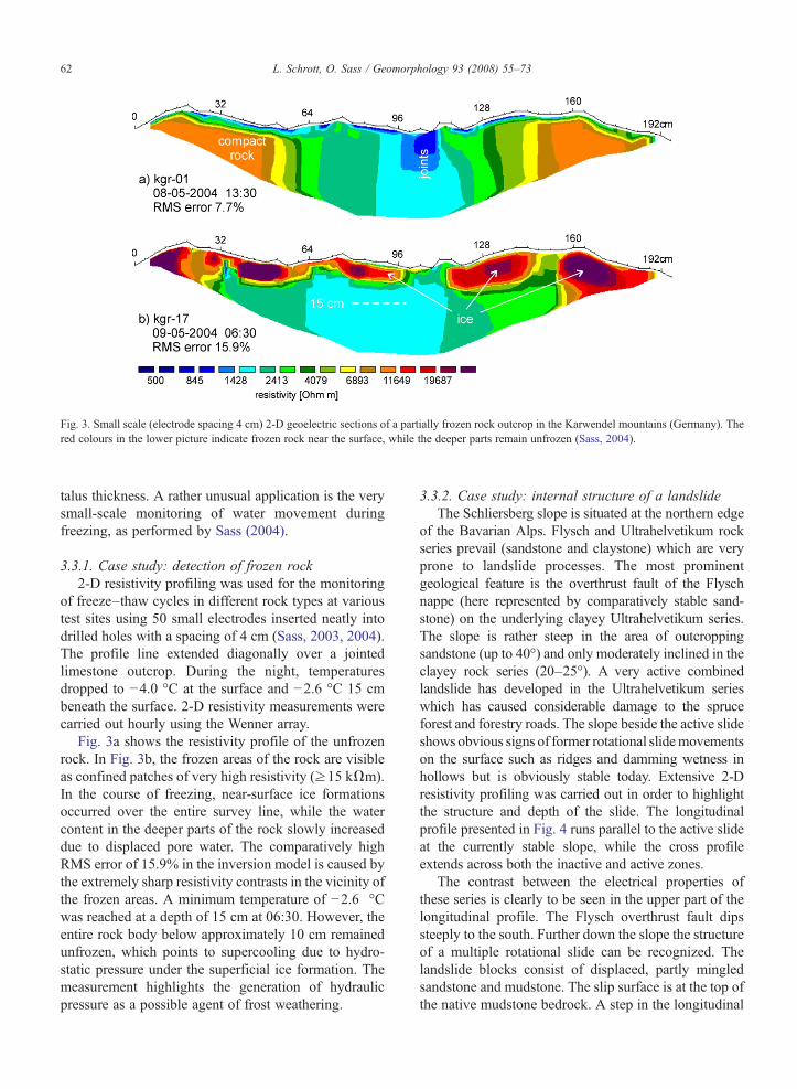
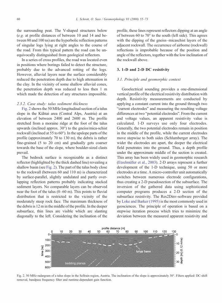
Fig. 3. Small scale (electrode spacing 4 cm) 2-D geoelectric sections of a partially frozen rock outcrop in the Karwendel mountains (Germany). Thered colours in the lower picture indicate frozen rock near the surface, while the deeper parts remain unfrozen (Sass, 2004).


talus thickness. A rather unusual application is the verysmall-scale monitoring of water movement duringfreezing, as performed by Sass (2004).

3.3.1. Case study: detection of frozen rock2-D resistivity profiling was used for the monitoring

of freeze–thaw cycles in different rock types at varioustest sites using 50 small electrodes inserted neatly intodrilled holes with a spacing of 4 cm (Sass, 2003, 2004).The profile line extended diagonally over a jointedlimestone outcrop. During the night, temperaturesdropped to −4.0 °C at the surface and −2.6 °C 15 cmbeneath the surface. 2-D resistivity measurements werecarried out hourly using the Wenner array.

Fig. 3a shows the resistivity profile of the unfrozenrock. In Fig. 3b, the frozen areas of the rock are visibleas confined patches of very high resistivity (≥15 kΩm).In the course of freezing, near-surface ice formationsoccurred over the entire survey line, while the watercontent in the deeper parts of the rock slowly increaseddue to displaced pore water. The comparatively highRMS error of 15.9% in the inversion model is caused bythe extremely sharp resistivity contrasts in the vicinity ofthe frozen areas. A minimum temperature of −2.6 °Cwas reached at a depth of 15 cm at 06:30. However, theentire rock body below approximately 10 cm remainedunfrozen, which points to supercooling due to hydro-static pressure under the superficial ice formation. Themeasurement highlights the generation of hydraulicpressure as a possible agent of frost weathering.

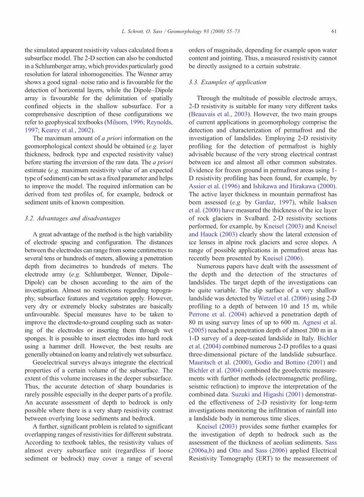
3.3.2. Case study: internal structure of a landslideThe Schliersberg slope is situated at the northern edge

of the Bavarian Alps. Flysch and Ultrahelvetikum rockseries prevail (sandstone and claystone) which are veryprone to landslide processes. The most prominentgeological feature is the overthrust fault of the Flyschnappe (here represented by comparatively stable sand-stone) on the underlying clayey Ultrahelvetikum series.The slope is rather steep in the area of outcroppingsandstone (up to 40°) and only moderately inclined in theclayey rock series (20–25°). A very active combinedlandslide has developed in the Ultrahelvetikum serieswhich has caused considerable damage to the spruceforest and forestry roads. The slope beside the active slideshows obvious signs of former rotational slidemovementson the surface such as ridges and damming wetness inhollows but is obviously stable today. Extensive 2-Dresistivity profiling was carried out in order to highlightthe structure and depth of the slide. The longitudinalprofile presented in Fig. 4 runs parallel to the active slideat the currently stable slope, while the cross profileextends across both the inactive and active zones.

The contrast between the electrical properties ofthese series is clearly to be seen in the upper part of thelongitudinal profile. The Flysch overthrust fault dipssteeply to the south. Further down the slope the structureof a multiple rotational slide can be recognized. Thelandslide blocks consist of displaced, partly mingledsandstone and mudstone. The slip surface is at the top ofthe native mudstone bedrock. A step in the longitudinal

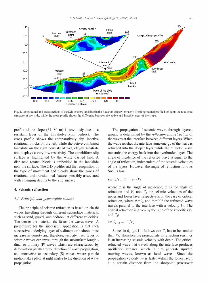
Fig. 4. Longitudinal and cross sections of the Schliersberg landslide in the Bavarian Alps (Germany). The longitudinal profile highlights the rotationalstructure of the slide, while the cross profile shows the difference between the active and inactive areas of the slope.


profile of the slope (64–80 m) is obviously due to aresistant layer of the Ultrahelvetikum bedrock. Thecross profile shows the comparatively dry, inactiverotational blocks on the left, while the active combinedlandslide on the right consists of wet, clayey substrateand displays a very low resistivity. The conchiform slipsurface is highlighted by the white dashed line. Adisplaced rotated block is embedded in the landslidenear the surface. The 2-D profiles aid the recognition ofthe type of movement and clearly show the zones ofrotational and translational features possibly associatedwith changing depths to the slip surface.

4. Seismic refraction


The principle of seismic refraction is based on elasticwaves travelling through different subsurface materials,such as sand, gravel, and bedrock, at different velocities.The denser the material, the faster the waves travel. Aprerequisite for the successful application is that eachsuccessive underlying layer of sediment or bedrock mustincrease in density and therefore, velocity. Two types ofseismic waves can travel through the subsurface: longitu-dinal or primary (P) waves which are characterized bydeformation parallel to the direction of wave propagation,and transverse or secondary (S) waves where particlemotion takes place at right angles to the direction of wavepropagation.

The propagation of seismic waves through layeredground is determined by the reflection and refraction ofthe waves at the interface between different layers. Whenthe wave reaches the interface some energy of the wave isrefracted into the deeper layer, while the reflected wavetransmits the energy back into the overburden layer. Theangle of incidence of the reflected wave is equal to theangle of reflection, independent of the seismic velocitiesof the layers. However the angle of refraction followsSnell's law:

sin hi=sin hr ¼ V1=V2

where θi is the angle of incidence, θr is the angle ofrefraction and V1 and V2 the seismic velocities of theupper and lower layer respectively. In the case of criticalrefraction, where θi=θc and θr=90° the refracted wavetravels parallel to the interface with a velocity V2. Thecritical refraction is given by the ratio of the velocities V1

and V2:

sin hc1;2 ¼ V1=V2:

Since sin θc1,2≤1 it follows that V1 has to be smallerthan V2. Therefore the prerequisite in refraction seismicsis an increasing seismic velocity with depth. The criticalrefracted wave that travels along the interface producesoscillation stresses, which in turn generate upwardmoving waves, known as head waves. Since thepropagation velocity V2 is faster within the lower layer,at a certain distance from the shotpoint (crossover


distance) these head waves reach the surface (geophones)faster than the direct wave providing the first arrivals atthe geophones. In seismic refraction studies, it is the firstarrivals of the P waves that are utilized.

The seismic velocity of P waves is dependent on theelastic modulus and the density, ρ, of the material,through which the seismic waves propagate.

Based on the raypath geometry described above and thestructure of the layered underground, it follows that thetravel times for the seismic waves can be used to obtaincertain time–distance plots. In the case of a layeredundergroundwith planar interfaces, the first arrival times lieon a number of clearly defined straight-line segments. Thenumber of the segments corresponds to the number of theunderground layers. The slope of the straight line segmentsis proportional to the reciprocal velocity of the layers.Travel time anomalies are caused by irregularities of theinterfaces and varying velocities within the different layers.

The arrival of a seismic wave is detected by geophones,which are placed firmly in the ground using a spacing ofbetween 1 and 5 m. For example, 24 geophones (with a 24channel seismograph) combined with a spacing of 4 mresults in a spread of 92 m. If the expected depths of theinterfaces are shallower than 30 m the geophone spacingmay be reduced (i.e. between 1 and 3 m) to gain a higherresolution record of the underground. To detect a layerwithin the time–distance plot the geophone spacing mustbe smaller than the difference between two followingcrossover distances. At the crossover distance the directwave is overtaken by a refracted wave. Beyond this offsetdistance the first arrival is always a refracted wave. Inrefraction surveying, recording ranges are chosen to besufficiently large enough to ensure that the crossoverdistance is well exceeded in order to detect a sufficientnumber of first arrivals of refracted waves. In cases of thinsubsurface layers, where the distance between crossoverpoints is small, a narrowgeophone spacing (between 1 and3 m) is necessary. This in turn may result in a lowerpenetration depth due to a reduced total spread.

The most common seismic source in geomorpholog-ical studies is a 5 kg sledge hammer which generatesseismic waves by hitting a metal plate placed on theground. To improve the signal to noise ratio the sledgehammer “shot” is usually repeated several times (typicallybetween 5 and 10 times) at the same source spot. Theresulting seismograms of each shot are stacked (summed)manually or automatically to obtain a single seismogramper shot location.

Generally, a sledge hammer is sufficient tomeasure thefirst arrivals along offset distances of approx. 50 m andseldom more than 90 m. This corresponds to penetrationdepths of 10 to 30 m and is suitable for many landforms.

More powerful sources (e.g. drop weights, explosives)must be used for longer surveys with larger penetrationdepths. To apply seismic surveys in geomorphic studies itis highly recommended to use instruments with severalsingle light units rather than to use an all-in-one (heavy)seismograph.

4.2. Advantages and disadvantages

The accurate first onset detection of seismic waves isvery often a difficult task. In coarse grained surfaceconditions (i.e. on talus slopes and debris cones) andhummocky topography (i.e. on rock glaciers or rockfalldeposits) difficulties may arise from the poor coupling ofgeophones to the surface. On talus slopes with largerblock sizes directly on the talus surface, it is advisable toimprove the coupling of the geophones by removing theupper layer of larger boulders and pushing the spike of thegeophone into fine-grained material underneath. Cou-pling to larger boulders or to compact bedrock may beestablished by drilling into the rock and plunging thespike within the drill hole.

In the vicinity of torrents and under strong wind orrainfall, the detection of seismic wavesmay be impossibledue to strong noise in the seismic record. Special attentionshould be drawn to the obtained velocities of materialswhich are common in particular landforms (e.g. talusdeposit, till, rock glacier). The large range of observedvelocity values, spanning from ∼400 m/s (loose debris)up to 6500 m/s (compact rocks) is generally conducive tothe application of refraction seismics, as large velocitycontrasts between the underlying materials are necessary.However, ranges of P wave velocities for rocks andsediments can overlap significantly. For instance, seismicvelocities of dolomite and limestone can vary between2000 and 6500 m/s depending on the grade of fracturingand weathering, while, for example, glacial sedimentscompacted by overlying ice can possibly range from 1500to 3500 m/s. Consequently, there is no unambiguousrelationship between certain subsurface units and thelinked P wave velocities. As a result, it is not alwayspossible to identify subsurface materials simply based onseismic velocities. To differentiate glacial till (without ice)from frozen ground or solid rock, cross checks with othergeophysical methods and/or evidence from boreholelogging are needed. Generally, landforms consisting ofsimilar sediments but deposited by different geomorphicprocesses cannot be distinguished (Hoffmann andSchrott, 2003). Another very common disadvantage inseismic refraction is the “hidden layer” problem, whichmay lead to incorrect interpretations (Pullan and Hunter,1990; Hecht, 2001). The hidden layer is caused by a

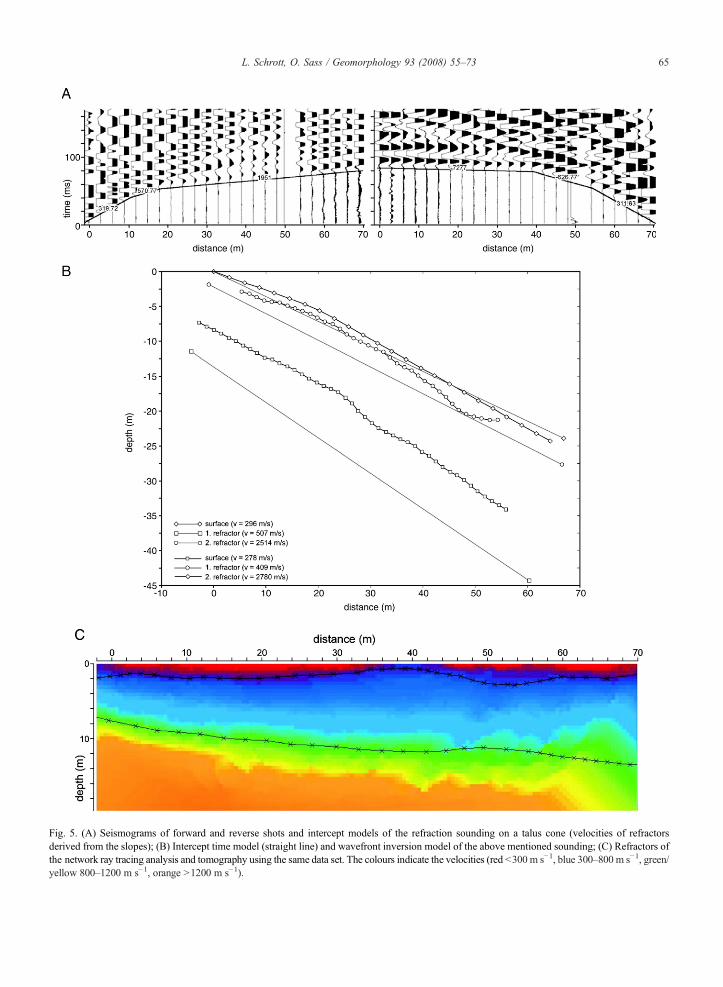
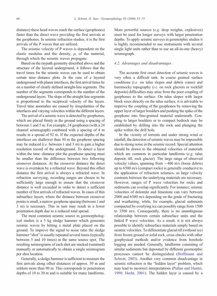
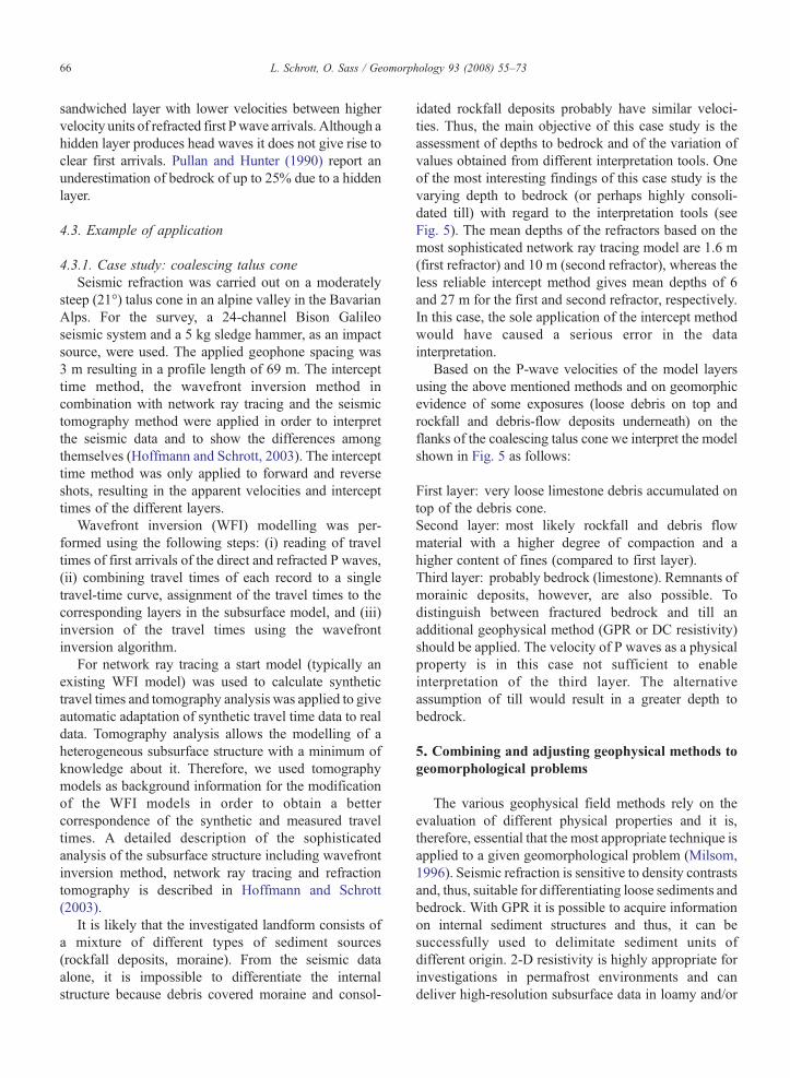
Fig. 5. (A) Seismograms of forward and reverse shots and intercept models of the refraction sounding on a talus cone (velocities of refractorsderived from the slopes); (B) Intercept time model (straight line) and wavefront inversion model of the above mentioned sounding; (C) Refractors ofthe network ray tracing analysis and tomography using the same data set. The colours indicate the velocities (red b300 m s−1, blue 300–800 m s−1, green/yellow 800–1200 m s−1, orange N1200 m s−1).



sandwiched layer with lower velocities between highervelocity units of refracted first Pwave arrivals. Although ahidden layer produces head waves it does not give rise toclear first arrivals. Pullan and Hunter (1990) report anunderestimation of bedrock of up to 25% due to a hiddenlayer.

4.3. Example of application

4.3.1. Case study: coalescing talus coneSeismic refraction was carried out on a moderately

steep (21°) talus cone in an alpine valley in the BavarianAlps. For the survey, a 24-channel Bison Galileoseismic system and a 5 kg sledge hammer, as an impactsource, were used. The applied geophone spacing was3 m resulting in a profile length of 69 m. The intercepttime method, the wavefront inversion method incombination with network ray tracing and the seismictomography method were applied in order to interpretthe seismic data and to show the differences amongthemselves (Hoffmann and Schrott, 2003). The intercepttime method was only applied to forward and reverseshots, resulting in the apparent velocities and intercepttimes of the different layers.

Wavefront inversion (WFI) modelling was per-formed using the following steps: (i) reading of traveltimes of first arrivals of the direct and refracted P waves,(ii) combining travel times of each record to a singletravel-time curve, assignment of the travel times to thecorresponding layers in the subsurface model, and (iii)inversion of the travel times using the wavefrontinversion algorithm.

For network ray tracing a start model (typically anexisting WFI model) was used to calculate synthetictravel times and tomography analysis was applied to giveautomatic adaptation of synthetic travel time data to realdata. Tomography analysis allows the modelling of aheterogeneous subsurface structure with a minimum ofknowledge about it. Therefore, we used tomographymodels as background information for the modificationof the WFI models in order to obtain a bettercorrespondence of the synthetic and measured traveltimes. A detailed description of the sophisticatedanalysis of the subsurface structure including wavefrontinversion method, network ray tracing and refractiontomography is described in Hoffmann and Schrott(2003).

It is likely that the investigated landform consists ofa mixture of different types of sediment sources(rockfall deposits, moraine). From the seismic dataalone, it is impossible to differentiate the internalstructure because debris covered moraine and consol-

idated rockfall deposits probably have similar veloci-ties. Thus, the main objective of this case study is theassessment of depths to bedrock and of the variation ofvalues obtained from different interpretation tools. Oneof the most interesting findings of this case study is thevarying depth to bedrock (or perhaps highly consoli-dated till) with regard to the interpretation tools (seeFig. 5). The mean depths of the refractors based on themost sophisticated network ray tracing model are 1.6 m(first refractor) and 10 m (second refractor), whereas theless reliable intercept method gives mean depths of 6and 27 m for the first and second refractor, respectively.In this case, the sole application of the intercept methodwould have caused a serious error in the datainterpretation.

Based on the P-wave velocities of the model layersusing the above mentioned methods and on geomorphicevidence of some exposures (loose debris on top androckfall and debris-flow deposits underneath) on theflanks of the coalescing talus cone we interpret the modelshown in Fig. 5 as follows:

First layer: very loose limestone debris accumulated on
top of the debris cone. Second layer: most likely rockfall and debris flow material with a higher degree of compaction and ahigher content of fines (compared to first layer). Third layer: probably bedrock (limestone). Remnants of morainic deposits, however, are also possible. Todistinguish between fractured bedrock and till anadditional geophysical method (GPR or DC resistivity)should be applied. The velocity of P waves as a physicalproperty is in this case not sufficient to enableinterpretation of the third layer. The alternativeassumption of till would result in a greater depth tobedrock.
5. Combining and adjusting geophysical methods togeomorphological problems

The various geophysical field methods rely on theevaluation of different physical properties and it is,therefore, essential that the most appropriate technique isapplied to a given geomorphological problem (Milsom,1996). Seismic refraction is sensitive to density contrastsand, thus, suitable for differentiating loose sediments andbedrock. With GPR it is possible to acquire informationon internal sediment structures and thus, it can besuccessfully used to delimitate sediment units ofdifferent origin. 2-D resistivity is highly appropriate forinvestigations in permafrost environments and candeliver high-resolution subsurface data in loamy and/or


wooded terrain whereas GPR frequently fails to deliverany data at all.

Thus, each of the geophysical methods presented has agreat potential for aiding clarification of geomorpholog-ical problems (Table 2). Nonetheless, everymethod has itsdrawbacks and limitations. The main reason for incom-plete or false conclusions lies in a lack of contrast betweenthe physical properties of the subsurface layers, particu-larly between compacted or water-saturated sedimentsand bedrock. With regard to the common problem ofdifferentiating loose debris from the bedrock base, it canbe stated that (1) there might be no distinct dielectricalcontrast and thus, no radar reflection at the bedrocksurface, (2) the electrical resistivity of debris can vary byorders of magnitude, which means that contrasts withinthe sediment body may exceed and mask the contrast tothe bedrock, and (3) the seismic velocities of compactedsediment such as basal moraine may overlap the velocityrange of bedrock, thus producing potential errors in thedetection of the sediment base. To overcome these

Table 2Common geophysical methods in geomorphological applications andqualitative assessment in terms of suitable detection of thickness and/or internal structure

Ground-penetratingradar

2-D DCresistivity

2-D seismicrefraction

Physical property Dielectricalproperties

Resistivity Elasticmoduli,density

Geomorphic contextTalus slopes, debris cones ++ a/++ b ±/+ ++ a/± b

Block fields +/+ ±/o +/oAlluvial fans, floodplain +/++ +/+ ++/±Colluvial +/+o +/o ±/–Landslides – c/± c +/++ ±/±Karst features ± o oPermafrost lenses + ++ ±Active layer thickness ± ++ ++Permafrost occurrence

(widespread)+ ++ +

Rock glaciers ±/+ ±/++ ± d

Rock/soil moisturedistribution

± + –

Note: the indication of suitable application may be incorrect underspecific or extreme local conditions (e.g. wet, dry and blocky).(++ very recommended, + recommended, ± may be used but notnecessarily the best approach, o has not been widely used or developedfor geomorphic application, – unsuitable).a Thickness, depth-to-bedrock.b Internal structure/distribution.c Only suitable in dry sediments.d Unsuitable on active rock glaciers with a permafrost body.

problems it is strongly advised that two or moregeophysical methods are used whenever possible.

5.1. Composite application on talus slopes

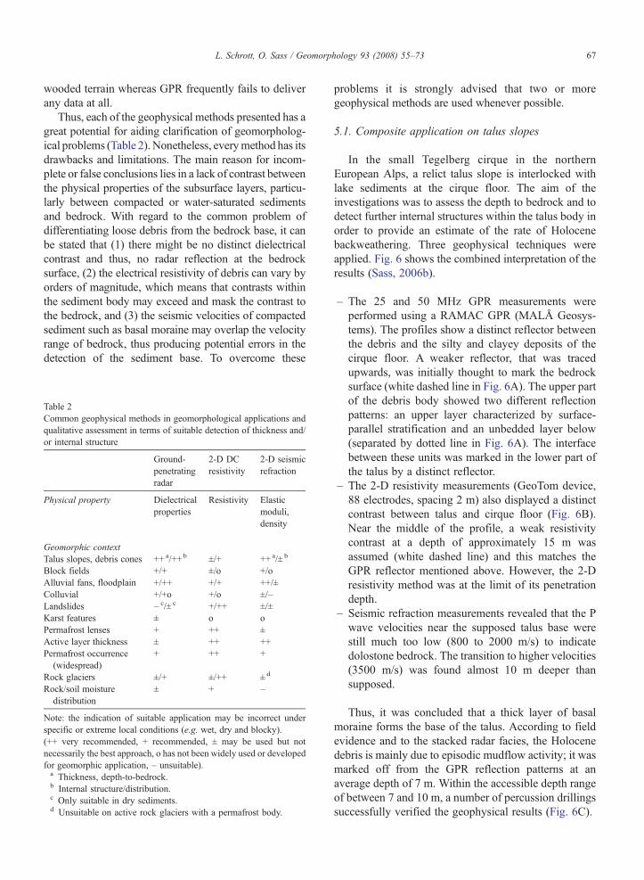
In the small Tegelberg cirque in the northernEuropean Alps, a relict talus slope is interlocked withlake sediments at the cirque floor. The aim of theinvestigations was to assess the depth to bedrock and todetect further internal structures within the talus body inorder to provide an estimate of the rate of Holocenebackweathering. Three geophysical techniques wereapplied. Fig. 6 shows the combined interpretation of theresults (Sass, 2006b).

– The 25 and 50 MHz GPR measurements wereperformed using a RAMAC GPR (MALÅ Geosys-tems). The profiles show a distinct reflector betweenthe debris and the silty and clayey deposits of thecirque floor. A weaker reflector, that was tracedupwards, was initially thought to mark the bedrocksurface (white dashed line in Fig. 6A). The upper partof the debris body showed two different reflectionpatterns: an upper layer characterized by surface-parallel stratification and an unbedded layer below(separated by dotted line in Fig. 6A). The interfacebetween these units was marked in the lower part ofthe talus by a distinct reflector.

– The 2-D resistivity measurements (GeoTom device,88 electrodes, spacing 2 m) also displayed a distinctcontrast between talus and cirque floor (Fig. 6B).Near the middle of the profile, a weak resistivitycontrast at a depth of approximately 15 m wasassumed (white dashed line) and this matches theGPR reflector mentioned above. However, the 2-Dresistivity method was at the limit of its penetrationdepth.

– Seismic refraction measurements revealed that the Pwave velocities near the supposed talus base werestill much too low (800 to 2000 m/s) to indicatedolostone bedrock. The transition to higher velocities(3500 m/s) was found almost 10 m deeper thansupposed.

Thus, it was concluded that a thick layer of basalmoraine forms the base of the talus. According to fieldevidence and to the stacked radar facies, the Holocenedebris is mainly due to episodic mudflow activity; it wasmarked off from the GPR reflection patterns at anaverage depth of 7 m. Within the accessible depth rangeof between 7 and 10 m, a number of percussion drillingssuccessfully verified the geophysical results (Fig. 6C).

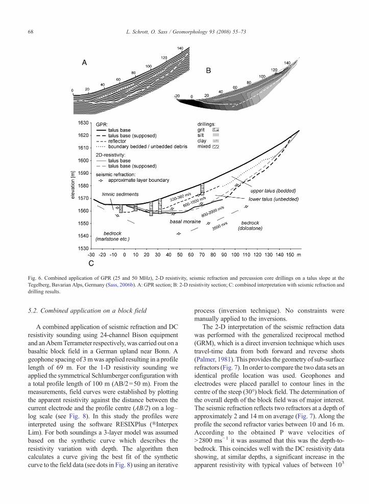
Fig. 6. Combined application of GPR (25 and 50 MHz), 2-D resistivity, seismic refraction and percussion core drillings on a talus slope at theTegelberg, Bavarian Alps, Germany (Sass, 2006b). A: GPR section; B: 2-D resistivity section; C: combined interpretation with seismic refraction anddrilling results.


5.2. Combined application on a block field

A combined application of seismic refraction and DCresistivity sounding using 24-channel Bison equipmentand anAbemTerrameter respectively, was carried out on abasaltic block field in a German upland near Bonn. Ageophone spacing of 3mwas applied resulting in a profilelength of 69 m. For the 1-D resistivity sounding weapplied the symmetrical Schlumberger configuration witha total profile length of 100 m (AB/2=50 m). From themeasurements, field curves were established by plottingthe apparent resistivity against the distance between thecurrent electrode and the profile centre (AB/2) on a log–log scale (see Fig. 8). In this study the profiles wereinterpreted using the software RESIXPlus (®InterpexLim). For both soundings a 3-layer model was assumedbased on the synthetic curve which describes theresistivity variation with depth. The algorithm thencalculates a curve giving the best fit of the syntheticcurve to the field data (see dots in Fig. 8) using an iterative

process (inversion technique). No constraints weremanually applied to the inversions.

The 2-D interpretation of the seismic refraction datawas performed with the generalized reciprocal method(GRM), which is a direct inversion technique which usestravel-time data from both forward and reverse shots(Palmer, 1981). This provides the geometry of sub-surfacerefractors (Fig. 7). In order to compare the two data sets anidentical profile location was used. Geophones andelectrodes were placed parallel to contour lines in thecentre of the steep (30°) block field. The determination ofthe overall depth of the block field was of major interest.The seismic refraction reflects two refractors at a depth ofapproximately 2 and 14 m on average (Fig. 7). Along theprofile the second refractor varies between 10 and 16 m.According to the obtained P wave velocities ofN2800 ms−1 it was assumed that this was the depth-to-bedrock. This coincides well with the DC resistivity datashowing, at similar depths, a significant increase in theapparent resistivity with typical values of between 103

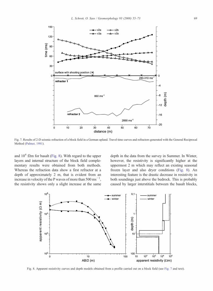
Fig. 7. Results of 2-D seismic refraction of a block field in a German upland. Travel time curves and refractors generated with the General ReciprocalMethod (Palmer, 1981).


and 104 Ωm for basalt (Fig. 8). With regard to the upperlayers and internal structure of the block field comple-mentary results were obtained from both methods.Whereas the refraction data show a first refractor at adepth of approximately 2 m, that is evident from anincrease in velocity of the Pwaves ofmore than 500ms−1,the resistivity shows only a slight increase at the same

Fig. 8. Apparent resistivity curves and depth models obtained from

depth in the data from the survey in Summer. In Winter,however, the resistivity is significantly higher at theuppermost 2 m which may reflect an existing seasonalfrozen layer and also dryer conditions (Fig. 8). Aninteresting feature is the drastic decrease in resistivity inboth soundings just above the bedrock. This is probablycaused by larger interstitials between the basalt blocks,

a profile carried out on a block field (see Fig. 7 and text).


interflows and accumulated downwashed clay mineralswhich may lead to very low resistivities. This interpre-tation, however, remains speculative and requires furtherfield evidence. In particular a two-dimensional soundingwould help to improve the interpretation. Both methodsdelivered similar results for estimations of the depths tobedrock.

6. Conclusions

Geophysical techniques have rendered it possibleto obtain many new and stimulating solutions forgeomorphological problems during the last decade.Geophysics, as used by geomorphologists, shouldbecome a common tool within geomorphology, butshould not marginalise the geomorphological question.Thus, there is a need for studies coupling thegeophysical background with geomorphic approachesin different natural environments and for differentlandforms.

A number of studies have provided new insights inmany landform and process related topics, for example,active layer, internal structure of rock glaciers and talusslopes, depth and extension of landslide bodies andsediment thickness. As previously pointed out, eachtechnique is sensitive to contrasts in certain physicalproperties which in turn reflect different sedimentcharacteristics (see Table 2). Ground-penetrating radarhas been successfully applied in permafrost studies,depth to bedrock, and for soil moisture measurement,but is particularly suitable for assessment of internalsedimentary structures (especially in sediment unitswith size fractions larger than silt). In these environ-ments, radar wave reflectivity is determined by contrastsin water content that are directly influenced by grain sizecomposition.

2-D resistivity measurements are particularly prom-ising in areas where there are strong contrasts inelectrical resistivity such as permafrost and landslides.It is probably best suited for isolated bodies such aspermafrost (Kneisel et al., 2000) or ice lenses andlandslide structures. Sledge hammer seismic refraction isparticularly recommended for shallow applications(b30m) in environments with mostly horizontal beddingand strong differences in P wave velocities such as drytalus slopes with loose debris above bedrock.

Further investigations using integrated approaches arerequired. Only an appropriate combination of differingmethods allows for much more sophisticated datainterpretation. Attention should be paid, not only to thethickness, but also to the internal structure of loosedeposits — a task that can only be can be achieved in

sufficient accuracy with the combination of severalmethods. Furthermore, a multi-method approach allowsfor cross-checking of results and determination of thesuitable methods for achieving valuable and reliableresults in a particular environment.

The consideration of some general recommendations(“best practice guide”) may help to avoid incorrect andunsuccessful geophysical applications and interpreta-tions in geomorphic research and to improve signifi-cantly the accuracy of gathered data:

1. Before using field geophysics, attempt to obtain asmuch information as possible about expected subsur-face conditions such as lithology, soil thickness,groundwater, and depth-to-bedrock as this maysignificantly influence the measurement strategy. ForGPR, DC resistivity and seismic refraction techniquesthe information may influence the choice of antennafrequency, electrode array and seismic refractionrespectively.

2. For reliable interpretation of survey results, availableknowledge of, for example, depth of a particularsediment, hollows, ice lenses and depth of ground-water at geomorphological and geological sites isessential. This a priori information may significantlyimprove post-processing in terms of creating ade-quate starting models or defining boundary condi-tions such as expected depth to bedrock and type ofbedrock).

3. Always ask the question: Is the geophysical modelgeomorphologically and/or geologically plausible?

4. Do not strictly adhere to the measurement strategy.Whenever possible, vary the applied frequency orelectrode configuration. The results are often surprising.

5. Never trust in a single method. Combine—wheneverpossible — two or three methods. Cross-checking isessential to increase the trustworthiness of the datainterpretation.

6. A geophysical method never provides a uniquesolution to a particular geomorphic situation, but mayhelp to improve the interpretation.

7. Check and validate results with, where possible,investigations of wells, exposures, borehole–logs ordrillings.

8. If there are not any exposures at the study site (whichmay be, in fact, the very reason for your applicationof geophysics), try to obtain test profiles under moreor less known subsurface conditions somewhere inthe vicinity of the site. Knowing the physicalproperties or reflection patterns of typical sedimentsin your study area will significantly facilitate yourinterpretation.


9. Find a geophysicist who is interested in geomorpho-logical approaches and discuss critical data andmodelling strategies during the post-processing.

Acknowledgments

The authors are grateful to numerous students from theUniversities ofAugsburg andBonn for their support in thefield. Special thanks to Thomas Hoffmann for criticaldiscussions on an earlier draft of this paper. We gratefullyacknowledge many valuable comments by two anony-mous reviewers and a thorough revision by oneanonymous referee that substantially improved themanuscript. Jonathan Mole's English corrections aregreatly appreciated. We are also grateful to all themembers of the research programme “Sediment Cascadesin Alpine Geosystems” (SEDAG) for co-operative fieldwork. Financial support from the Deutsche Forschungs-gemeinschaft is greatly appreciated (grant Schr 648/1-3).

References

Agnesi, V., Camardo, M., Conoscenti, C., Dimaggio, C., Diliberto,I.S., Madonia, P., Rotigliano, E., 2005. Amultidisciplinary approachto the evaluation of the mechanism that triggered the Cerda landslide(Sicily, Italy). Geomorphology 65, 101–116.

Arcone, S.A., Lawson, D.E., Delaney, A.J., Strasser, J.C., 1998.Ground-penetrating radar reflection profiling of groundwater andbedrock in an arctic discontinuous permafrost. Geophysics 63,1573–1584.

Assier, A., Fabre, D., Evin, M., 1996. Prospection électrique sur lesglaciers rocheux du cirque de Sainte-Anne (Queyras, Alpes duSud, France). Permafrost and Periglacial Processes 7, 53–67.

Baker, J.A., Anderson, N.L, Pilles, P.J., 1997. Ground-penetratingradar surveying in support of archaeological site investigations.Computers and Geosciences 23, 1093–1099.

Beauvais, A., Ritz, M., Parisot, J.-C., Bantsimba, C., 2003. Testingetching hypothesis for the shaping of granite dome structuresbeneath lateritic weathering landforms using ERT method. EarthSurface Processes and Landforms 28, 1071–1080.

Berthling, I., Etzelmüller, B., Isaksen, K., Sollid, J.L., 2000. Rockglaciers on Prins Karls Forland. II: GPR Soundings and theDevelopment of Internal Structures, vol. 11, pp. 357–369.

Bichler, A., Bobrowsky, P., Best, M., Douma, M., Hunter, J., Calvert, T.,Burns, R., 2004. Three-dimensional mapping of a landslide using amulti-geophysical approach: the Quesnel Forks landslide. Landslides1, 29–40.

Bristow, C.S., Bailey, S.D., Lancaster, N., 2000. The sedimentarystructure of linear sand dunes. Nature 406, 56–59.

Bruno, F., Mariller, F., 2000. Test of high-resolution seismic reflectionand other geophysical techniques on the Boup landslide in theSwiss Alps. Surveys in Geophysics 21, 333–348.

Büker, F., Gurtner, M., Horstmeyer, H., Green, A.G., Huggenberger, P.,1996. Three-dimensional mapping of glaciofluvial and deltaicsediments in central Switzerland using ground penetrating radar.Proceedings of the “Sixth International Conference on GroundPenetrating Radar”, Sendai, Japan, pp. 45–50.

Doolittle, J.A., Collins, M.E., 1995. Use of soil information todetermine application of ground penetrating radar. Journal ofApplied Geophysics 33, 101–108.

Etzelmüller, B., Berthling, I., Odegard, R.S., 2003. One-dimensionalDC-resistivity depth soundings as a tool in permafrost investiga-tions in high mountain areas of Southern Norway. Zeitschrift fürGeomorphologie. N.F., Supplementband 132, 19–36.

Fuchs, G., Hruska, J., 1996. Die Georadar-Methode in der arch-äologischen Prospektion. Archäologie Österreichs 7, 71–79.

Fuchs, M., Zöller, L., 2006. Geoarchäologie aus geomorphologischerSicht. Eine konzeptionelle Betrachtung. Erdkunde 60, 139–146.

Gardaz, J.-M., 1997. Distribution of Mountain Permafrost, Fonta-nesses Basin, Valaisian Alps, Switzerland. Permafrost andPeriglacial Processes 8, 101–105.

Gilbert, R. (Ed.), 1999. A handbook of geophysical techniques forgeomorphic and environmental research. Geological survey ofCanada, open file 3731 in collaboration with the CanadianGeomorphological Research Group (with contributions from M.Douma, L. Dyke, R. Gilbert, R.L. Good, J.A. Hunter, C. Hyde, Y.Michaud, S.E. Pullan, and S.D. Robinson), 125 pp.

Godio, A., Bottino, G., 2001. Electrical and electromagnetic investiga-tion for landslide characterisation. Physics and Chemistry of theEarth. Part C: Solar-Terrestrial and Planetary Science 26, 705–710.

Hauck, C., 2001. Geophysical methods for detecting permafrost inhigh mountains. Mitt. Versuchanstalt für Wasserbau, Hydrologieund Glaziologie. ETH Zürich, vol. 171. 204 pp.

Hauck, C., Vonder Mühll, D., 2003. Evaluation of geophysicaltechniques for application in mountain permafrost studies. Zeitschriftfür Geomorphologie. N.F., Supplementband 132, 161–190.

Hecht, S., 2000. Fallbeispiele zur Anwendung refraktionsseismischerMethoden bei der Erkundung des oberflächennahen Untergrundes.Zeitschrift für Geomorphologie. N.F., Supplementband 123, 111–123.

Hecht, S., 2001. Anwendung refraktionsseismischer Methoden zurErkundung des oberflächennahen Untergrundes. Stuttgarter Geo-graphische Studien 131 165 pp.

Hecht, S., 2003. Investigation of the shallow subsurface with seismicrefraction methods — application potentials and limitations withexamples from various field studies. Zeitschrift für Geomorpho-logie. N.F., Supplementband 132, 19–36.

Hinkel, K.M., Doolittle, J.A., Bockheim, J.G., Nelson, F.E., Paetzold,R., Kimble, J.M., 2001. Detection of subsurface permafrostfeatures with ground-penetrating radar, Barrow, Alaska. Perma-frost and Periglacial Processes 12, 179–190.

Hoffmann, T., Schrott, L., 2002. Modelling sediment thickness androckwall retreat in an Alpine valley using 2D-seismic refraction(Reintal, Bavarian Alps). Zeitschrift für Geomorphologie. N.F.,Supplementband 127, 175–196.

Hoffmann, T., Schrott, L., 2003. Determining sediment thickness oftalus slopes and valley fill deposits using seismic refraction — acomparison of 2D interpretation tools. Zeitschrift für Geomorpho-logie. N.F., Supplementband 132, 71–87.

Holden, J., Burt, T.P., Vilas, M., 2002. Application of ground-penetrating radar to the identification of subsurface piping inblanket peat. Earth Surface Processes and Landforms 27, 235–249.

Isaksen, K., Ødegård, R.S., Eiken, T., Sollid, J.L., 2000. Composition,flow and development of two tongue-shaped rock glaciers in thepermafrost of Svalbard. Permafrost and Periglacial Processes 11,241–257.

Ishikawa, M., Hirakawa, K., 2000. Mountain permafrost distributionbased on BTS measurements and DC resistivity soundings in theDaisetsu Mountains, Hokkaido, Japan. Permafrost and PeriglacialProcesses 11, 109–123.


Israil, M., Pachauri, A.K., 2003. Geophysical characterization of alandslide site in the Himalayan foothill region. Journal of AsianEarth Sciences 22, 253–263.

Jol, H.M., 1996. Three-dimensional GPR imaging of a fan-foresetdelta: an example from Brigham City, Utah, USA. Proc. of the 6thInternational Conference on Ground Penetrating Radar (GPR '96),Sendai, Japan, pp. 33–37.

Jol, H.M., Bristow, C.S., 2003. GPR in sediments: advice on datacollection, basic processing and interpretation, a good practiceguide. In: Bristow, C.S., Jol, H.M. (Eds.), Ground-penetratingRadar in Sediments. Geological Society London, Special Publica-tion, vol. 211, pp. 177–185.

Kearey, P., Brooks, M., Hill, I., 2002. An Introduction to GeophysicalExploration. Blackwell, London. 262 pp.

Kneisel, C., 2003. Electrical resistivity tomography as a tool forgeomorphological investigations — some case studies. Zeitschriftfür Geomorphologie. N.F., Supplementband 132, 37–49.

Kneisel, C., 2006. Assessment of subsurface lithology in periglacial envi-ronments using 2D resistivity imaging. Geomorphology 80, 32–44.

Kneisel, C., Hauck, C., 2003. Multi-method geophysical investigationof a sporadic permafrost occurrence. Zeitschrift für Geomorpho-logie. N.F., Supplementband 132, 145–159.

Kneisel, C., Hauck, C., Vonder Mühll, D., 2000. Permafrost below thetimberline confirmed and characterized by geoelectrical resistivitymeasurements, Bever Valley, Eastern Swiss Alps. Permafrost andPeriglacial Processes 11, 295–304.

Leckebusch, J., 2003. Ground-penetrating radar: a modern three-dimensional prospection method. Archaeological Prospection 10,213–240.

Leclerc, R.F., Hickin, E.J., 1997. The internal structure of scrolledfloodplain deposits based on ground-penetrating radar, NorthThompson River, British Columbia. Geomorphology 21, 17–25.

Loke, M.H., Barker, R.D., 1995. Least-squares deconvolution ofapparent resistivity. Geophysics 60, 1682–1690.

Lønne, I., Lauritsen, T., 1996. The architecture of a modern push-moraine at Svalbard as inferred from ground-penetrating radarmeasurements. Arctic and Alpine Research 28, 488–495.

Loope, W.L., Fisher, T.G., Jol, H.M., Goble, R.J., Anderton, J.B.,Blewett, W.L., 2004. A Holocene history of dune-mediatedlandscape change along the southeastern shore of Lake Superior.Geomorphology 61, 303–322.

Mauritsch, H.J., Seiberl, W., Arndt, R., Römer, A., Schneiderbauer, K.,Sendlhofer, G.P., 2000. Geophysical investigations of largelandslides in the Carnic region of southern Austria. EngineeringGeology 56, 373–388.

Milsom, J., 1996. Field Geophysics. Wiley, Chichester. 187 pp.Moorman, B.J., Michel, F.A., 2000. Glacial hydrological system

characterization using ground-penetrating radar. HydrologicalProcesses 14, 2645–2667.

Moorman, B.J., Robinson, S.D., Burgess, M.M., 2003. Imagingperiglacial conditions with ground-penetrating radar. Permafrostand Periglacial Processes 14, 319–329.

Otto, J.C., Sass, O., 2006. Comparing geophysical methods for talusslope investigations in the Turtmann valley (Swiss Alps).Geomorphology 76, 257–272.

Overgaard, T., Jakobsen, P.R., 2001. Mapping of glaciotectonicdeformation in an ice marginal environment with groundpenetrating radar. Journal of Applied Geophysics 47, 191–197.

Palmer, D., 1981. An introduction to the generalized reciprocal methodof seismic refraction interpretation. Geophysics 46, 1508–1518.

Perrone, A., Iannuzzi, A., Lapenna, V., Lorenzo, P., Piscitelli, S.,Rizzo, E., Sdao, F., 2004. High-resolution electrical imaging of the

Varco d'Izzo earthflow (southern Italy). Journal of AppliedGeophysics 56, 17–29.

Pullan, S.E., Hunter, J.A., 1990. Delineation of buried bedrock valleysusing the optimum offset shallow seismic reflection technique. In:Ward, S.H. (Ed.), Geotechnical and Environmental Geophysiscs,V.III, Geotechnical. Society of Exploration Geophysicists, Tulsa,Oklahoma, pp. 75–87.

Reynolds, J.M., 1997. An Introduction to Applied and EnvironmentalGeophysics. Wiley, Chichester. 778 pp.

Roberts, M.C., Bravard, J.-P., Jol, H.M., 1997. Radar signatures andstructures of an avulsed channel: Rhone river, Aoste, France.Journal of Quaternary Science 12, 35–42.

Sass, O., 2003. Moisture distribution in rockwalls derived from 2D-resistivity measurements. Zeitschrift für Geomorphologie. N.F.,Supplementband 132, 51–69.

Sass, O., 2004. Rockmoisture fluctuations during freeze–thaw cycles—preliminary results derived from electrical resistivity measurements.Polar Geography 28, 13–31.

Sass, O., 2006. Determination of the internal structure of alpine talususing different geophysical methods (Lechtaler Alps, Austria).Geomorphology 80, 45–58.

Sass, O., 2006. Geophysical investigation of a relict talus slope in theBavarian Alps, Germany. Zeitschrift für Geomorphologie 50,447–463.

Sass, O., Wollny, K., 2001. Investigations regarding alpine talus slopesusing ground penetrating radar (GPR) in the Bavarian Alps,Germany. Earth Surface Processes and Landforms 26 (10),1071–1086.

Sass, O., Schneider, T., Wollny, K., 2004. Die frührömische Holz-Kies-Straβe im Murnauer Moos - Untersuchung des ehemaligenVerlaufs mittels Georadar (GPR). Mitteilungen der MünchenerGeographischen Gesellschaft 87, 275–293.

Sass, O., Bell, R., Glade, T., 2008. Comparison of GPR, 2D-resistivityand traditional techniques for the subsurface exploration of theÖschingen landslide, Swabian Alb (Germany). Geomorphology93, 89–103 (this issue). doi:10.1016/j.geomorph.2006.12.019.

Schrott, L., Pfeffer, G., Möseler, B.M., 2000. GeophysikalischeUntersuchungen an einer Blockhalde im Mittelgebirge (Hunds-bachtal, Eifel). Acta Universitatis Purkynianae. Studia Biologica 4,19–30.

Schrott, L., Hufschmidt, G., Hankammer, M., Hoffmann, T.,Dikau, R., 2003. Spatial distribution of sediment storage typesand quantification of valley fill deposits in an upper Alpinebasin, Reintal, Bavarian Alps, Germany. Geomorphology 55,45–63.

Schwamborn, G.J., Dix, J.K., Bull, J.M., Rachold, V., 2002. Highresolution seismic and ground-penetrating radar geophysicalprofiling of a thermokarst lake in the western Lena Delta, NorthernSiberia. Permafrost and Periglacial Processes 13, 259–269.

Smith, D.G., Jol, H.M., 1995. Ground penetrating radar: antennafrequencies and maximum probable depths of penetration inQuaternary sediments. Journal of Applied Geophysics 33, 93–100.

Suzuki, K., Higashi, S., 2001. Groundwater flow after heavy rain inlandslide-slope area from 2D-inversion of resistivity monitoringdata. Geophysics 66, 733–743.

Tavkhelidse, T., Schulte, A., Stumböck, M., Schuhkraft, G., 2000.Aufbau und Entwicklung der Schuttkegel im Finkenbachtal,Südlicher Odenwald. Jenaer Geographische Schriften 9,95–110.

Topp, G.C., Davis, J.L., Annan, A.P., 1980. Electromagneticdetermination of soil water content: measurements in coaxialtransmission lines. Water Resources Research 16, 574–582.


Van der Kruk, J., Slob, E.C., 2004. Reduction of reflections fromabove surface objects in GPR data. Journal of Applied Geophysics55, 271–278.

Völkel, J., Leopold, M., Roberts, M.C., 2001. The radar signatures andage of periglacial slope deposits, Central Highlands of Germany.Permafrost and Periglacial Processes 12, 379–387.

Wetzel, K.-F., Sass, O., Restorff, C., 2006. Mass movement processesin unconsolidated Pleistocene sediments — a multi-method

investigation at the “Hochgraben” (Jenbach / Upper Bavaria).Erdkunde 60, 246–260.

Wollny, K.G., 1999. Die Natur der Bodenwelle und ihr Einsatz zurFeuchtebestimmung. PhD thesis, Faculty of Geoscience, Ludwig-Maximilians-Universität, Munich.

Documents

Application of field geophysics in geomorphology: Advances