Available online at www.sciencedirect.com

Journal of the Franklin Institute 350 (2013) 2982–2993

0016-0032/$3http://dx.doi.o

nCorresponE-mail ad

www.elsevier.com/locate/jfranklin

Application of functional derivatives to analysisof complex systems

Zdeněk Berann, Sergej ČelikovskýInstitute of Information Theory and Automation, v.v.i., Academy of Sciences of the Czech Republic,

Pod vodárenskou věží 4, P.O. Box 18, 182 08 Prague 8, Czech Republic

Received 9 October 2012; received in revised form 7 February 2013; accepted 6 April 2013Available online 25 April 2013

Abstract

The application of the functional derivatives to the mathematical modeling of complex systems is studiedhere. The connection of functional derivatives with total differentials in Banach spaces is shown. Local andglobal existence theorems for the linear equations in total differentials are proved. Consequently, a totalintegrability conditions are derived for the case of linear equations with the functional derivatives. Someillustrative examples are included.& 2013 The Franklin Institute. Published by Elsevier Ltd. All rights reserved.

1. Introduction

The theory of the equations in total differentials in Banach spaces has a long history and thistheory occupies a visible place in nearly any textbook devoted to the theory of differentialequations (see, e.g., [1–4]). On the contrary, the theory of the equations with functionalderivatives is greatly deficient though the application area of that kind of equations is quitebroad. Let us mention the area of quantum field theory (e.g., [5–7]), the statistical theory ofturbulence (e.g., [8–11]), the area of chemical kinetics (e.g., [12,13]), last but not least, the areaof mechanical engineering and numerical mathematics, see, e.g., [14].Very likely, the reason of the above-mentioned contradiction is that the theory of the equations

in total differentials takes independent variables mainly from the n-dimensional Euclidean vectorspace while the theory of the equations with functional derivatives takes independent variablesfrom functional spaces, making a subsequent analysis incredibly difficult. In fact, only few

2.00 & 2013 The Franklin Institute. Published by Elsevier Ltd. All rights reserved.rg/10.1016/j.jfranklin.2013.04.007

ding author. Tel.: +420 728 713 434.dresses: beran@utia.cas.cz (Z. Beran), celikovs@utia.cas.cz (S. Čelikovský).

Z. Beran, S. Čelikovský / Journal of the Franklin Institute 350 (2013) 2982–2993 2983

general results were published for the case of rather narrow classes of equations with functionalderivatives (see, e.g., [15–18]). The rest of results deals with entirely individualistic types of theequations. The solutions of equations with functional derivatives are sought very often by “trial-and-error” method or some procedures, like the separation of variables or the theory ofcharacteristics. These procedures stem from the theory of ODEs or PDEs.

The functional derivatives have their own remarkable significance relevant to various areas ofscience and engineering. Let us mention just two of them.

First, the sensitivity theory deals usually with a response of the system solutions tolocal changes of some parameter(s). The functional derivatives approach allows one tostudy the sensitivity of the system with respect to whole classes of functions. An application tothe reliability analysis can be found in, e.g., [14,19], and the literature cited withinthere.

Second, the functional derivatives approach lies in the background of a very usefularea, namely, in the background of the so-called density functional theory (DFT). DFT has itsorigin already in, e.g., [10,11], and the literature quoted within there. It is worth to mention alsothe following classical source that covers different topics in the statistical mechanicsof non-uniform, classical fluids [20]. Today, the DFT has a very broad applications in particletheory, chemical kinetics, quantum chemistry, etc. In the DFT, the functional derivativesform a base when using a variational approach to evaluate the ground state density in multi-particles quantum systems and molecular dynamics. One of the common approaches uses theKohn–Sham equations facilitating directly the practical calculations. During the recent decades,several DFT theories were developed and adapted to different problems of the multi-particles'theories, see, e.g., [21,22]. The application area is very broad today, see, e.g., [23–28]. The DFThas been also expanded from the stationary case to the time-dependent DFT, as one can found in,e.g., [29,30].

We concentrate ourself to the case of the linear equations with total differentials because thesubsequent applications of this linear case is sufficient for our applications. Local and globalexistence results for the equations in total differentials defined on general Banach spaces will bederived thereby implying the results for the case of the equations with functional derivatives.Finally, the procedure and conditions of derivation of the functional derivatives will be describedbased on the concept of total differentials.

The rest of the paper is organized as follows. Basic definitions are summarized in Section 2,while Section 3 contains the main results of the paper being the existence results for theequations in total differentials defined on general Banach spaces. Section 4 demonstrates theabove-mentioned procedure and conditions for the case of equations with functional derivativesand conditions are shown under which that equations are equivalent to the equations in totaldifferentials. Section 5 gives illustrative examples, while the final section draws someconclusions and gives some outlooks for the future research.

2. Preliminaries

Let us first recall some necessary definitions and facts [31–33]. We suppose that allBanach spaces introduced later on are separable when needed. Let E be a real Banach space andF be a real or complex Banach space. Further, LðE;FÞ stands for the Banach space oflinear bounded mappings with the norm ∥A∥¼ sup∥x∥ ¼ 1∥Ax∥ and suppose that U⊂E is anopen set.

Z. Beran, S. Čelikovský / Journal of the Franklin Institute 350 (2013) 2982–29932984

Definition 1. A mapping f : U-F is called Frèchet differentiable at the point x∈U if thereexists a linear bounded operator Ax∈LðE;FÞ such that

limΔx-0

∥f ðxþ ΔxÞ−f ðxÞ−AxΔx∥∥Δx∥

¼ 0:

The operator Ax is called as the total differential or Frèchet differential at the point x∈U. We willdenote it as f ′ðxÞ.Let the function f be differentiable at all points of the set U, then the mapping f ′ : U-LðE;FÞ

is defined. Let the mapping f ′ be continuous, then the function f is called as continuouslydifferentiable on U, or, as of class C1. Further, assume that the mapping f ′ is differentiableon U, then there exists a mapping (the second differential) f ″¼ ðf ′Þ′ : U-LðE; LðE;FÞÞ. Thespace LðE; LðE;FÞÞ is naturally identified with the space L2ðE;FÞ of bilinear mappingsE � E-F.Consider a pair of Banach spaces E1 and E2 and a mapping f : E1 � E2-F. The partial

differentials are defined as the differentials of the mappings x1-f ðx1; x2Þ and x2-f ðx1; x2Þ.Further consider a functional F : CðDÞ-R, where C(D) is the space of continuous functions,D⊂R being the domain of their definition. Suppose this functional is Gateaux differentiable atsome point x0∈CðDÞ along h∈CðDÞ, i.e., its Gateaux derivative

δF ðx0; hÞ ¼ limϵ-0

F ðx0 þ ϵhÞ−F ðx0Þϵ

exists and it is a continuous linear functional on C(D). Moreover, as a consequence of the Rieszrepresentation theorem there exists a regular countably additive measure μf ;x0 defined on thealgebra of closed subsets of D such that

δF ðx0; hÞ ¼ZDhðtÞ dμf ;x0 ;

where 0oϵ∈R.

Definition 2. Suppose

δF ðx0; hÞ ¼ZDψF ðx0; tÞhðtÞ dt;

where the function t-ψF ðx0; tÞ is at least integrable on D. The function ψF ðx0; tÞ is called as thefunctional derivative of functional F at the point x0∈CðDÞ and it is denoted as

δF ðx0ÞδxðtÞ :

Definition 3. Suppose U ¼U � V⊂E � F is an open set in E � F and g : U-LðE;FÞ is acontinuous mapping. Differential equation

y′¼ gðx; yÞ ð1Þdefines the equation in total differentials for a Frèchet differentiable function y with respect to theindependent variable x.

As already noted, let us further restrict ourselves to the case of linear equations, i.e., thefunction y-gðx; yÞ is affine for all x∈U. This means that Eq. (1) becomes

y′¼ BðxÞyþ f ðxÞ; ð2Þ

Z. Beran, S. Čelikovský / Journal of the Franklin Institute 350 (2013) 2982–2993 2985

where B : U-LðF; LðE;FÞÞ is continuous function, the function f maps U into LðE;FÞ. Wesuppose that V¼F. The spaces LðF; LðE;FÞÞ and LðE; LðF;FÞÞ can be mutually identified andeach operator B∈LðF; LðE;FÞÞ can be identified with an operator A∈LðE; LðF;FÞÞ by the ruleByh¼Ahy for every h∈E and y∈F. Then, the mapping B-A defines an isomorphism betweenBanach spaces LðF; LðE;FÞÞ and LðE; LðF;FÞÞ, moreover, Eq. (2) can be re-written as follows:

y′h¼ AðxÞhyþ f ðxÞh ∀h∈E: ð3Þ

Definition 4. A solution of Eq. (3) is any single-valued function y : Q-F of the class C1, whichis defined on the open set Q⊂U and satisfies the equation y′ðxÞh¼ AðxÞhyðxÞ þ f ðxÞh; h∈E forevery x∈Q.

Definition 5. Eq. (3) is said to be totally integrable or totally solvable on the open set U⊂E, iffor arbitrary point ðx0; y0Þ∈U � F there exists a unique solution y of Eq. (3) which is defined insome neighborhood Q of the point x0 and satisfies the initial condition

yðx0Þ ¼ y0: ð4ÞDefinition 6. Let C∈L2ðE;FÞ be an arbitrary bilinear operator. The operation of taking theskewed symmetric part of the bilinear operator C is defined as follows:

⋀Chk ¼ 12ðChk−CkhÞ ∀h; k∈E: ð5Þ

Definition 7. Let L be an arbitrary two-dimensional space in E and let Sðx0; δh; δkÞ be thetriangle in ðx0 þ LÞ∩U with vertices x0; x0 þ δh; x0 þ δk, where h; k∈L, and with the boundary

Γ ¼ x0 ðx0 þ δhÞ ðx0 þ δhÞ ðx0 þ δkÞ ðx0 þ δkÞ x0 :The curl of a function A at the point x0∈U is a bilinear operator curl Aðx0Þ : E2-LðE;FÞ suchthat

curl Aðx0Þhk¼ limδ-þ0

1

δ2

ZΓAðsÞ ds ð6Þ

uniformly for arbitrary h; k∈bð0; 1Þ∩L, where bð0; 1Þ is the unit ball in E.

Note that if the curl exists, then it is uniquely defined and the operator curl Aðx0Þ is skewsymmetric.

In the next section, we will need two lemmas (see [31, pp. 170–174]). To formulate theselemmas, let us first introduce some notation. On an oriented closed curve Γ consider the orderingdetermined by the orientation of p points x1;…; xp. Further, connect these points to a point x0outside Γ or on Γ by means of curves li ¼ x0xi ∀ i¼ 1;…; p. The expression l−1i ¼ xix0 stands forthe curve reciprocal to li. The curves li; liþ1; i¼ 0; 1; 2;…;modðpÞ and the arc xi; xiþ1 of Γ forma closed curve Γi, which can be described as the sequence x0xixiþ1x0 from x0 to x0. Then (settingTΓi ¼ Ti;PΓi ¼ Pi and Tli ¼ Ti)

TΓ ¼ TlTp…TlTl−1 :

When Ti ¼ I þ Pi is introduced, then for PΓ ¼ TΓ−I one obtains the expansion

PΓ ¼ Tl ∑p

i ¼ 1Si

� �Tl−1 ;

Z. Beran, S. Čelikovský / Journal of the Franklin Institute 350 (2013) 2982–29932986

where Si ¼∑Pj1…Pji is taken over all combinations p≥j1≥⋯≥ji≥1. As the products of thetransformations P are in general not commutative the factors in the individual terms of this summust be taken in the indicated order.

Lemma 1. Suppose the operator A(x) is continuous in domain U and for each point x0∈U andfor each fixed plane L⊂E such that x0∈L it holds

limSðx;h;kÞ-x0

PΓ

Δðx; h; kÞ ¼ 0:

Here, the triangle Sðx; h; kÞ ¼ Sðx1; x2; x3Þ with boundary Γ in L is meant to converge regularly tox0∈S while Δ¼Dhk; h¼ x2−x1; k¼ x3−x1 denotes the real fundamental form of the plane S⊂Lso that Δ represents the oriented area of the triangle. Then the integrability condition PΓ ¼ 0holds for every closed, piecewise regular curve in the region U.

Lemma 2. Suppose the operator A(x) is differentiable at the point x0. Further supposeS¼ Sðx1; x2; x3Þ is a triangle with a boundary Γ in a neighborhood containing the point x0, δ isthe greatest side length. Then

PΓ ¼ Rðx0Þhk þ oðδ2Þ ¼⋀ A′ðx0Þhk−Aðx0ÞhAðx0Þkð Þ þ oðδ2Þ:Here, for the sake of brevity we put h¼ x2−x1; k¼ x3−x1.

3. Linear equations in total differentials

In this section, we prove the local existence theory for the homogenous equation (3), i.e., whenfunction f ðxÞ ¼ 0. The non-homogenous case will follow as its consequence. After that, we willprove the global existence theorem. First, we formulate the following local existence theorem:

Theorem 1. Let U⊂E be an open set and suppose the function A is differentiable in U. Then theequation

y′h¼ AðxÞhy; h∈E ð7Þis totally integrable in U if and only if the function A(x) has the curl at each point x∈U and theequality

curl AðxÞhk−⋀AðxÞhAðxÞk¼ 0 ∀h; k∈E ð8Þholds at each point x∈U.

Proof. ð⟹). Let x0∈U, let L be an arbitrary two-dimensional set in E and h; k∈bð0; 1Þ∩L. Then,obviously, for δ40 small enough, the triangle Sðx0; δh; δkÞ lies inside ðx0 þ LÞ∩U and thefunction A is (due to its continuity) bounded in some closed ball bðx0; ρx0 Þ⊂U, which contains thetriangle Sðx0; δh; δkÞ. Let on the boundary

Γ0 ¼ x0ðx0 þ δhÞðx0 þ δkÞx0of the triangle S0ðx0; δh; δkÞ it holds

PΓ0y0 ¼ZΓ0

AðvÞ dv z½v�;

where z is the solution of Eq. (7) along the curve Γ0 with the initial condition z½x0� ¼ y0; y0∈F.As the function A(x) is differentiable at the point x0∈U, one can write AðxÞ ¼Aðx0Þ þ A′ðx0Þðx−x0Þ þ oð∥x−x0∥Þ. Moreover, as z½v� ¼ y0 þ Aðx0Þðv−x0Þy0 þ oðδÞy0 with

Z. Beran, S. Čelikovský / Journal of the Franklin Institute 350 (2013) 2982–2993 2987

arbitrary y0,

PΓ0 ¼ZΓ0

AðvÞ dvþZΓ0

Aðx0Þ dv Aðx0Þðv−x0Þ þZΓ0

½AðvÞ−Aðx0Þ� dv Aðx0Þðv−x0Þ þ oðδ2Þ

¼ZΓ0

AðvÞ dv−⋀Aðx0ÞhAðx0Þkδ2 þ oðδ2Þ: ð9Þ

where δ¼ ∥x−x0∥. Now, using Lemma 1, we have

0¼ limδ-þ0

PΓ0

Δðx0; δh; δkÞ¼ lim

δ-þ0

PΓ0

δ2¼ lim

δ-þ0

1

δ2

ZΓ0

AðvÞ dv−⋀Aðx0ÞhAðx0Þk� �

;

which implies that the function A has the curl at the point x0 and Eq. (8) is granted.ð⇐). Let x0∈U be an arbitrary point and let ρx040 be a real number such that the ball bðx0; ρx0 Þ

lies entirely inside U including its closure bðx0; ρx0Þ and let the function A is bounded onbðx0; ρx0 Þ (A is differentiable thus continuous on a closed set). Let L⊂E be an arbitrary two-dimensional space and let the set of triangles Sðx; h; kÞ converges to the point x0 in ðx0 þLÞ∩bðx0; ρx0Þ assuming that the point x0 lies inside each triangle of the set Sðx; h; kÞ. As

PΓ ¼ZΓAðvÞ dv−⋀Aðx0ÞhAðx0Þk þ oðδ2Þ;

where Γ ¼ xðxþ hÞðxþ kÞx, then using of Eq. (8) and of Lemma 2, one gets

limSðx;h;kÞ-x0

PΓ

δ2¼ lim

Sðx;h;kÞ-x0

1

δ2

ZΓAðvÞ dv−curl Aðx0Þhk

� �¼ 0;

which, due to Lemma 1, implies the total integrability of Eq. (7). □

The non-homogenous case is solved in the following theorem.

Theorem 2. Let U⊂E be an open set and suppose the functions AðxÞ; BðxÞ∈C1ðUÞ. Then theequation

y′h¼ AðxÞhyþ BðxÞh; h∈E ð10Þis totally integrable in U if and only if

⋀fA′ðxÞhk−AðxÞhAðxÞkg ¼ 0 ∀h; k∈E ð11Þ

⋀fAðxÞhBðxÞk−B′ðxÞhkg ¼ 0 ∀h; k∈E ð12Þhold at each point x∈U.

Proof. The presumptions on the functions AðxÞ;BðxÞ imply that y∈C2ðUÞ. When differentiatingEq. (10), one gets

y″ðxÞhk¼ A′ðxÞkhyðxÞ þ AðxÞhAðxÞkyðxÞ þ AðxÞkBðxÞhþ B′ðxÞkh:As the mapping y″ðxÞ : E2-F is symmetric for each x∈U, it follows that the skewed symmetricpart

⋀fA′ðxÞkhyþ AðxÞhAðxÞkyþ AðxÞkAðxÞhþ B′ðxÞkhg ¼ 0

for each h; k∈E. The above equation is obviously equivalent to the two following equations:

⋀fA′ðxÞhk−AðxÞhAðxÞkg ¼ 0 ∀h; k∈E ð13Þ

Z. Beran, S. Čelikovský / Journal of the Franklin Institute 350 (2013) 2982–29932988

⋀fAðxÞhBðxÞk−B′ðxÞhkg ¼ 0 ∀h; k∈E ð14Þfor each point x∈U. The theorem has been proven. □

Prior to formulate the global existence theorem we introduce the environment we will work in.Let S be a set of connected subsets of the set U. We introduce, as usual, the ordering on that setby inclusion, i.e., we introduce in S a structure of the partial ordering according to the rule S1≤S2iff S1DS2. Consider any linearly ordered subset S′⊂S, such that the union ⋃S∈S′S⊂S.Let us have totally integrable equation

y′h¼ AðxÞhyþ f ðxÞh ∀h∈E ð15Þin an open set U⊂E, let the functions A : U-LðE; LðE;FÞÞ and f : U-LðE;FÞ be continuous.For arbitrary pair ðx0; y0Þ∈U � F there exists (due to Theorem 1) a solution y, which is definedinside the ball bðx0; ρx0 Þ and satisfies the initial condition yðx0Þ ¼ y0. We would like to extend thesolution y from the ball bðx0; ρx0Þ onto a larger set. As the larger set has to be also the set where,at the same time, the solution is defined, we introduce a pair (y,S), S⊂U, defining the solution ofEq. (15). Actually, this solution is given by the open set S⊂U being the definition domain of thesolution and of the differentiable function y : S-F solving Eq. (15).

Definition 8. Let (y,S) be a solution of Eq. (15). An extension of that solution is the solutionðy1; S1Þ for which S⊂S1 and yðxÞ ¼ y1ðxÞ for all x∈S.

Definition 9. The solution (y,S) of Eq. (15) is said to be non-extendable one in the class S if forarbitrary extension ðy1; S1Þ of that solution with S1∈S it holds that S1 ¼ S.

We formulate now the global existence theorem:

Theorem 3. Let ðx0; y0Þ∈U � F be an arbitrary point, then there exists a non-extendablesolution ðy; Sx0y0 Þ of Eq. (15) in the class S and x0∈Sx0y0 ; yðx0Þ ¼ y0.

Proof. Let us define the set

Sx0y0 ¼ fS∈Sjx0∈S;∃ yS : S-F; ðyS; SÞ solves ð15Þ with ySðx0Þ ¼ y0g:On Sx0y0 we introduce a partial ordering, which is induced from S, and we will show that eachlinearly ordered set S′⊂Sx0y0 has a majorant. Let

S0 ¼ ⋃S∈S′

S: ð16Þ

One can see that x0∈S0 and S0∈S. We define a function yS0 : S0-F as follows: for arbitraryx∈S0 we set yS0 ðxÞ ¼ ySðxÞ when x∈S. As the set S′ is linearly ordered and the sets S∈S areconnected, the definition of the function yS0 is well posed. Moreover, yS0 satisfies Eq. (15) withthe initial condition yS0 ðx0Þ ¼ y0. Due to Eq. (16) the set S0 is a majorant for S′. According to theZorn lemma in the partially ordered set Sx0y0 there exists a maximal element, i.e., there existssuch Sx0y0∈Sx0y0 that the inclusion Sx0y0⊂S, S∈Sx0y0 implies that S¼ Sx0y0 . It means that thesolution ðy; Sx0y0Þ with the definition domain Sx0y0 is non-extendable in the class Sx0y0 and, thus, itis neither extendable in the class S. The proof is completed. □

Z. Beran, S. Čelikovský / Journal of the Franklin Institute 350 (2013) 2982–2993 2989

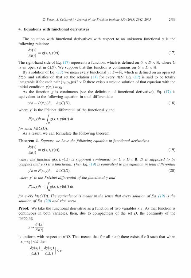
4. Equations with functional derivatives

The equation with functional derivatives with respect to an unknown functional y is thefollowing relation:

δyðxÞδxðtÞ ¼ gðx; t; yðxÞÞ: ð17Þ

The right-hand side of Eq. (17) represents a function, which is defined on U � D� R, where Uis an open set in C(D). We suppose that this function is continuous on U � D� R.

By a solution of Eq. (17) we mean every functional y : S-R, which is defined on an open setS⊂U and satisfies on that set the relation (17) for every t∈D. Eq. (17) is said to be totallyintegrable if for each pair ðx0; y0Þ∈U � R there exists a unique solution of that equation with theinitial condition yðx0Þ ¼ y0.

As the function g is continuous (see the definition of functional derivative), Eq. (17) isequivalent to the following equation in total differentials:

y′h¼ Pðx; yÞh; h∈CðDÞ; ð18Þwhere y′ is the Frèchet differential of the functional y and

Pðx; yÞh¼ZDgðx; t; yÞhðtÞ dt

for each h∈CðDÞ.As a result, we can formulate the following theorem:

Theorem 4. Suppose we have the following equation in functional derivatives

δyðxÞδxðtÞ ¼ gðx; t; yðxÞÞ; ð19Þ

where the function gðx; t; yðxÞÞ is supposed continuous on U � D� R, D is supposed to becompact and y(x) is a functional. Then Eq. (19) is equivalent to the equation in total differential

y′h¼ Pðx; yÞh; h∈CðDÞ; ð20Þwhere y′ is the Frèchet differential of the functional y and

Pðx; yÞh¼ZDgðx; t; yÞhðtÞ dt

for every h∈CðDÞ. The equivalence is meant in the sense that every solution of Eq. (19) is thesolution of Eq. (20) and vice versa.

Proof. We take the functional derivative as a function of two variables x; t. As that function iscontinuous in both variables, then, due to compactness of the set D, the continuity of themapping

x-δyðxÞδxðtÞ

is uniform with respect to t∈D. That means that for all ϵ40 there exists δ40 such that when∥x1−x2∥oδ then��� δyðx1Þ

δxðtÞ −δyðx2ÞδxðtÞ

���oϵ

Z. Beran, S. Čelikovský / Journal of the Franklin Institute 350 (2013) 2982–29932990

for each t∈D. It immediately implies that the mapping

h-

ZD

δyðxÞδxðtÞ hðtÞ dt¼ δyðx; hÞ∈R; h∈CðDÞ ð21Þ

defines the Frèchet differential y′ of the functional y. As the function G is continuous, then due toEq. (21), Eq. (19) is equivalent to Eq. (20) where Pðx; yÞh¼ R

Dgðx; t; yÞhðtÞ dt for every h∈CðDÞ.The theorem is proven. □

Thus, the problem of the analysis of the equations with functional derivatives is transformedinto the problem for the equations in total differentials. As we mentioned already, we target thelinear equations with functional derivatives. So, we will analyze the linear equation in functionalderivatives

δyðxÞδxðtÞ ¼ aðx; tÞyðxÞ þ bðx; tÞ ð22Þ

and we suppose that the functions a : U � D-R; b : U � D-R are continuous. Denote

AðxÞh¼ZDaðx; tÞhðtÞ dt; BðxÞh¼

ZDbðx; tÞhðtÞ dt; h∈CðDÞ: ð23Þ

Using Eq. (23), Eq. (22) can be re-written as the following equation in total differentials:

y′h¼ AðxÞhyþ BðxÞh; h∈E¼ CðDÞ ð24Þwith continuous functions A : U-CðDÞ; B : U-CðDÞ.Now, we can apply the results of the previous section to Eq. (24) to obtain the following:

Theorem 5. Suppose the functions a; b have continuous functional derivatives in U � D withrespect to x. Then Eq. (22) is totally integrable if and only if the following relations are satisfied:

δaðx; tÞδxðsÞ ¼ δaðx; sÞ

δxðtÞ ; ð25Þ

δbðx; tÞδxðsÞ þ aðx; sÞbðx; tÞ ¼ δbðx; sÞ

δxðtÞ þ aðx; tÞbðx; sÞ ð26Þ

for each x∈U and each s; t∈D.

Proof. Theorem 2 implies that Eq. (24) and thus the equivalent equation (22) are totallyintegrable if and only if the following relations are valid:

A′ðxÞhk¼ A′ðxÞkh; ð27Þ

⋀fAðxÞhBðxÞk−B′ðxÞhkg ¼ 0 ð28Þfor arbitrary h; k∈CðDÞ. Since

A′ðxÞhk¼ZD

ZD

δaðx; tÞδxðsÞ hðsÞkðtÞ ds dt;

it follows that Eq. (27) is equivalent to the relation (25). Similarly, Eq. (28) is equivalent to therelation (26). The theorem has been proven. □

Z. Beran, S. Čelikovský / Journal of the Franklin Institute 350 (2013) 2982–2993 2991

5. Examples

In this section, the following examples to illustrate the previous results are given.

Example 1. The Schrödinger equation in functional derivatives [5] is often used in the quantumfield theory. It has the following form:

iδyðxÞδxðtÞ ¼Hðt; xÞ; ð29Þ

where yðxÞ ¼ SðxÞΦ, Φ is a constant, S(x) is the scattering matrix of interaction with an intensityx; y(x) is the amplitude of the system state. The operator Hðt; xÞ is a generalized Hamiltonian andit is calculated via scattering matrix. The conditions of total integrability are expressed by

δHðt; xÞδxðsÞ ¼ δHðs; xÞ

δxðtÞ :

The solutions of that equation are expressed in the form

yðxÞ ¼ y0 þZ x

x0

Hðt; vÞ δv; yðx0Þ ¼ y0:

Example 2. Next example, see [34], follows from the Schwinger equation, when the Fouriertransformation is applied

δGðx; ξÞδxðtÞ ¼ δ ln ΦðxÞ

δxðtÞ −i

a2ð− ξj2 þ a2Þ

�� �Gðx; ξÞ;

�ð30Þ

where Φ is known characteristic functional of a random quantity, a is a positive constant,ξ¼ ðξ1; ξ2; ξ3Þ∈R3; ξ2 ¼ ξ21 þ ξ22 þ ξ23, x∈CðDÞ is an element of the space CðDÞ; D⊂R3; of realcontinuous functions, and G : CðDÞ � R3-ðRÞ is the unknown function. Eq. (30) plays animportant role in the theoretical physics, see [34].

Supposing that the function Φ is sufficiently smooth, we can apply Theorem 5. As a result, Eq.(30) is totally integrable and the solution set is done by

Gðx; ξÞ ¼ exp −Z x

0

δ ln ΦðvÞδvðtÞ −

i

a2ð ξj2−a2Þ�� �

δv

� �qðξÞ;

�ð31Þ

where qðξÞ ¼Gð0; ξÞ is the initial function. The functional integral (31) can be easily evaluated.As a result, the function G takes the form

Gðx; ξÞ ¼ 1ΦðxÞ exp

i

a2ð ξj2−a2Þ

ZDxðtÞ dt

�����qðξÞ:

�

6. Conclusion and outlooks

The connection between total differentials and functional derivatives has been used to analyzethe linear equations with first-order functional derivatives, very often used in different areas ofphysics, chemistry and engineering. Conditions when the solution of such equations exists werederived.

The area of equations with functional derivatives is still open and the results are mostly basedon some amount of erudition. The general theory of solutions of differential equations with

Z. Beran, S. Čelikovský / Journal of the Franklin Institute 350 (2013) 2982–29932992

functional derivatives is still missing though some primary results can be found mostly in thearea of quantum field theory models. Nevertheless, the problems are generally processed on thecase-by-case basis.

Acknowledgments

This work is supported by Czech Science Foundation through the research Grant no. 13-20433S.

References

[1] P. Hartman, Ordinary Differential Equations, John Wiley & Sons Inc., 1964.[2] V.I. Arnold, Ordinary Differential Equations, MIT, 1978.[3] J.M. Page, Ordinary Differential Equations, Macmillan & Comp., 1897.[4] E.L. Ince, Ordinary Differential Equations, Dover Publications, 1958 ISBN 0-486-60349-0.[5] N. Bogoliubov, D. Shirkov, Quantum Fields, Benjamin-Cummings, 1982 ISBN 0-8053-0983-7.[6] N. Bogoliubov, A.A. Logunov, A.I. Oksak, I.T. Todorov, General Principles of Quantum Field Theory, Kluwer

Academic Publishers, 1990 ISBN 978-0-7923-0540-8.[7] S. Weinberg, The Quantum Theory of Fields, vol. 1–3, Cambridge University Press, 1995.[8] R.M. Lewis, R.H. Kraichnan, A space-time functional formalism for turbulence, Communications on Pure and

Applied Mathematics 15 (1962) 397–411.[9] E. Hopf, Statistical hydromechanics and functional calculus, Journal of Rational Mechanics and ANALYSIS 1

(1952) 87–123.[10] A.S. Monin, A.M. Yaglom, Statistical Fluid Mechanics—vol 1: Mechanics of Turbulence, 1st edition, The MIT

Press, September 15, 1971.[11] A.S. Monin, A.M. Yaglom, Statistical Fluid Mechanics, Volume II: Mechanics of Turbulence (Dover Books on

Physics), Dover edition, Dover Publications, June 5, 2007.[12] D.K. Dacel, H. Rabitz, Sensitivity analysis of stochastic kinetic models, Journal of Mathematical Physics 25

(September (9)) (1984) 2716–2727.[13] M. Demiralp, H. Rabitz, Chemical kinetic functional sensitivity analysis: derived sensitivities and general

applications, Journal of Chemical Physics 75 (1981) 1810.[14] A. Pownuk, General Interval FEM Program Based on Sensitivity Analysis, Research Report No. 2007-06, The

University of Texas at El Paso Department of Mathematical Sciences Research Reports Series, The University ofTexas at El Paso, 2008.

[15] I.M. Koval'chuk, Linear equations with functional derivatives, Ukrainskii Matematicheskii Zhurnal 29 (1) (1977)99–105.

[16] M.S. Syavavko, P.P. Mel'nichak, A class of equations with functional derivatives, Ukrainskii MatematicheskiiZhurnal 26 (6) (1974) 99–105.

[17] A. Inoue, A Certain Functional Derivative Equation Corresponding to □uþ cuþ bu2 þ au3 ¼ g on Rdþ1,Proceedings of the Japan Academy Series A 65 (1989).

[18] A. Inoue, A tiny step towards functional derivative equations—a strong solution of the space-time Hopf equation, in:J.G. Heywood et al.(Ed.), The Navier–Stokes equations—II Theory and Numerical Methods, Springer LectureNotes in Mathematics, vol. 1530, , 1992, pp. 246–261.

[19] A. Pownuk, General interval FEM program based on sensitivity analysis method, in: 2nd Joint UTEP/NMSUWorkshop on Mathematics and Computer Science, University of Texas at El Paso, El Paso, Texas, November 17,2007.

[20] R. Evans, The nature of the liquid–vapour interface and other topics in the statistical mechanics of non-uniform,classical fluids, Advances in Physics 28 (2) (1979) 143–200.

[21] H. Eschrig, The Fundamentals of Density Functional Theory, Teubner, Stuttgart, 1996 ⟨http://www.ifw-dresden.de/institutes/itf/members-groups/helmut-eschrig/dft.pdf⟩.

[22] C. Fiolhais, F. Nogueira, M. Marques (Eds.), A Primer in Density Functional Theory, Springer-Verlag, Berlin,Heidelberg, 2003.

[23] P.W. Ayers, J.I. Rodriguez, Out of one, many—Using moment expansions of the virial relation to deduce universaldensity functionals from a single system, Canadian Journal of Chemistry 87 (2009) 1540–1545.

Z. Beran, S. Čelikovský / Journal of the Franklin Institute 350 (2013) 2982–2993 2993

[24] A.D. Becke, Density-functional thermochemistry. I. The effect of the exchange-only gradient correction, Journal ofChemical Physics 96 (February (3)) (1992) 2155–2160.

[25] S.J.A. van Gisbergen, J.G. Snijders, E.J. Baerends, Accurate density functional calculations on frequency-dependenthyperpolarizabilities of small molecules, Journal of Chemical Physics 109 (December (24)) (1998) 10657–10668.

[26] P.E. Lammert, Differentiability of Lieb functional in electronic density functional theory, International Journal ofQuantum Chemistry 107 (2007) 1943–1953.

[27] M.J. Uline, K. Torabi, D.S. Cortib, Homogeneous nucleation and growth in simple fluids. I. Fundamental issues andfree energy surfaces of bubble and droplet formation, Journal of Chemical Physics 133 (2010)174511-1–174511-15.

[28] M.J. Uline, K. Torabi, D.S. Cortib, Homogeneous nucleation and growth in simple fluids. II. Scaling behavior,instabilities, and the (n,v) order parameter, Journal of Chemical Physics 133 (2010) 174512-1–174512-13.

[29] M.A.L. Marques, et al., Time-Dependent Density Functional Theory, Springer-Verlag, Berlin, Heidelberg, 2006.[30] U. Lourderaj, M.K. Harbola, N. Sathyamurthy, Time-dependent density functional theoretical study of low lying

excited states of F2, Chemical Physics Letters 366 (2002) 88–94.[31] F. Nevanlinna, R. Nevanlinna, Absolute Analysis, Springer-Verlag, 1973.[32] J. Dieudonné, Treatise on Analysis, vols. I–III, Academic Press, 1976.[33] L. Schwartz, Analyse mathématique, vols. I, II, Hermann, 1967.[34] V. I. Tatarskii˘, Rasprostranenie Voln v Turbulentnoi˘ Atmosfere (Wave Propagation in Turbulent Atmosphere),

Moscow, Nauka, 1967.