Embed Size (px)
Citation preview

Application of geometric algebra
to theoretical molecularspectroscopy
Janne PesonenUniversity of Helsinki
Department of Chemistry
Laboratory of Physical Chemistry
P.O. BOX 55 (A.I. Virtasen aukio 1)
FIN-00014 University of Helsinki, Finland
Academic dissertation
To be presented, with the permission of the Faculty of Science of the University
of Helsinki for public criticism in the Main lecture hall A110 of the Department
of Chemistry (A.I. Virtasen aukio 1, Helsinki) December 13th, 2001, at 10
o’clock.
Helsinki 2001

Supervised by:
Professor Lauri Halonen
Department of Chemistry
University of Helsinki
Reviewed by:
Professor Folke Stenman
Department of Physics
University of Helsinki
and
Doctor Tuomas Lukka
Department of Mathematical Information Technology
University of Jyvaskyla
Discussed with:
Professor Jonathan Tennyson
Department of Physics and Astronomy
University College London
UK
ISBN 952-91-4134-3 (nid.)
ISBN 952-10-0225-5 (verkkojulkaisu, pdf)
http://ethesis.helsinki.fi
Helsinki 2001
Yliopistopaino
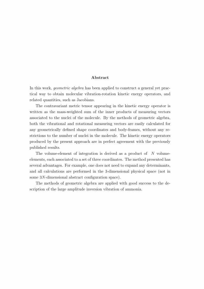
Abstract
In this work, geometric algebra has been applied to construct a general yet prac-
tical way to obtain molecular vibration-rotation kinetic energy operators, and
related quantities, such as Jacobians.
The contravariant metric tensor appearing in the kinetic energy operator is
written as the mass-weighted sum of the inner products of measuring vectors
associated to the nuclei of the molecule. By the methods of geometric algebra,
both the vibrational and rotational measuring vectors are easily calculated for
any geometrically defined shape coordinates and body-frames, without any re-
strictions to the number of nuclei in the molecule. The kinetic energy operators
produced by the present approach are in perfect agreement with the previously
published results.
The volume-element of integration is derived as a product of N volume-
elements, each associated to a set of three coordinates. The method presented has
several advantages. For example, one does not need to expand any determinants,
and all calculations are performed in the 3-dimensional physical space (not in
some 3N -dimensional abstract configuration space).
The methods of geometric algebra are applied with good success to the de-
scription of the large amplitude inversion vibration of ammonia.

Contents
1 Introduction 3
2 Geometric algebra 4
2.1 Introduction to basic concepts . . . . . . . . . . . . . . . . . . . . 5
2.2 Geometric transformations and relations . . . . . . . . . . . . . . 11
2.3 Quaternions . . . . . . . . . . . . . . . . . . . . . . . . . . . . . . 14
2.4 Geometric calculus . . . . . . . . . . . . . . . . . . . . . . . . . . 14
2.5 Some history and present . . . . . . . . . . . . . . . . . . . . . . . 18
3 Molecular Schrodinger equation 19
3.1 Born-Oppenheimer approximation . . . . . . . . . . . . . . . . . . 20
4 Kinetic energy operators for polyatomic molecules 20
4.1 Coordinate representation . . . . . . . . . . . . . . . . . . . . . . 21
4.2 Body-frames . . . . . . . . . . . . . . . . . . . . . . . . . . . . . . 27
4.3 Covariant measuring vectors and Lagrangian formulation . . . . . 29
5 Outlines for future research 30
1

List of publications
1. J. Pesonen, Vibrational coordinates and their gradients: A geometric alge-
bra approach. J. Chem. Phys. 112, 3121-3132 (2000).
2. J. Pesonen, Gradients of vibrational coordinates from the variation of co-
ordinates along the path of a particle. J. Chem. Phys. 115, 4402-4403
(2001).
3. J. Pesonen, A. Miani, and L. Halonen, New inversion coordinate for ammo-
nia: Application to a CCSD(T) bidimensional potential energy surface. J.
Chem. Phys. 115, 1243-1250 (2001).
4. J. Pesonen, Vibration-rotation kinetic energy operators: A geometric alge-
bra approach. J. Chem. Phys. 114, 10598-10607 (2001).
5. J. Pesonen and L. Halonen, Volume-elements of integration: A geometric
algebra approach. J. Chem. Phys, accepted for publication.
2

1 Introduction
I became first interested in molecular Hamiltonian operators while I browsed
through the book Molecular vibrations by Wilson, Decius and Cross. [1] The
authors present an ”s-vector” method for obtaining coordinate gradients (needed
to represent Laplacian operators in the Schrodinger equation) for standard shape
coordinates, such as bond lengths and valence angles. The gradients of the coor-
dinates ∇αqi were deduced from the change of the coordinate caused by the dis-
placement of the nucleus in question. But I was puzzled by two things. First, the
nuclei were assumed to move by unit displacements. But the authors were talking
about infinitesimal displacements, in which case there should not be any unit of
displacement! Second, I could not see if this method really produced a general ex-
pression for the gradient of the coordinate, or only the value ∇αqi
(q(e)1 , q
(e)2 , . . .
)of the gradient in terms of a reference configuration q
(e)1 , q
(e)2 , . . . used at the point
of displacement. Third, for a practical point of view this ”s-vector method”
seemed unsatisfactory, because the success of the method would depend if one
could somehow deduce the direction of greatest change in the coordinate caused
by the displacement of the nucleus in question. While this was easy for some
simple coordinates, it could be difficult for some more complicated coordinates.
The second impetus for my work was the inherent difficulties in finding the
rotation-vibration parts of kinetic energy operators. There existed a vast amount
of literature on the subject, but most of the solutions were solutions only in prin-
ciple, not in practice. This is especially true for those approaches concentrating
on the transformation from Lagrangian to (quantum mechanical) Hamiltonian.
They could in most cases be applied only to triatomic molecules. Some ap-
proaches for finding the vibration-rotation kinetic energy operator of an N -atomic
molecule appeared reasonable, because the body-fixed axes had been chosen in
terms of a tri-atomic fragment of the molecule. The only practical way presented
in the literature for finding the vibration-rotation kinetic energy operator (in
bond lengths and valence angles) was analogous to Wilson’s s-vector method.
This approach was invented by T. Lukka. It was based on the concept of in-
finitesimal rotations. [2] But for me the mathematical ground of the success of
this method was something of a mystery.
I finally concluded that the difficulties had their origin in the mathemati-
cal tools used in finding vibration-rotation kinetic energy operators. The tensor
analysis concentrates on coordinate transformations, which most part play no
3

intrinsic role in the problem at hand. Although solution could be obtained in
principle using tensor analysis, the intermediate expressions would fast become
intractable. On the other hand, the ordinary vector calculus is inappropriate for
the handling of rotations and just as in the case of tensor analysis the physical
concept of direction is separated from the algebraic operations. Thus, all the ap-
proaches utilizing physical displacement vectors or rotations as geometric entities
had to contain some heuristic steps to compensate the algebraic shortcomings in
the vector algebra. Clearly, to make any true progress, one would have to find
better mathematical tools. Geometric algebra, developed in the sixties by David
Hestenes, turned out to be such an ideal instrument. It also gave me the chance
to clearly pinpoint the conditions under which the ”s-vector” method would work
or fail in finding the coordinate gradients.
In this thesis, I apply geometric algebra to construct a general yet practical
way to obtain vibration-rotation kinetic energy operators and related quantities,
such as Jacobians. Paper 1 is devoted to the application of geometric algebra
to construction of exact vibrational kinetic energy operators. Geometric algebra
is used both to design suitable shape coordinates and to obtain the measuring
vectors needed to form the exact kinetic energy operators by the direct vectorial
differentiation of the coordinates. An alternative method to obtain the measuring
vectors is represented in Paper 2. An application of the method developed in
Paper 1 to the symmetric vibrational modes of ammonia is given in Paper 3. In
Paper 4, geometric algebra is used to obtain general yet practical formulas for the
rotational measuring vectors for any body-frame, without any restrictions to the
number of particles used to define the body-frame. In Paper 5, geometric algebra
is applied to find a practical way to obtain the volume-element of integration for
the 3 Cartesian coordinates of the center of mass, 3 Euler angles, and 3N − 6
shape coordinates needed to describe the position, orientation, and shape of an
N -atomic molecule.
2 Geometric algebra
Many distinct algebraic systems have been developed to express geometric rela-
tions. Among these are the well-established branches of complex analysis, matrix,
vector, and tensor algebras, and the less known calculus of differential forms, the
quaternion, and spinor algebras. Each of them has some advantage in certain ap-
4

plications and at the same time they overlap significantly, i.e. they provide several
mathematical representations of the same geometrical ideas. Geometric algebra
integrates all these algebraic systems to a coherent mathematical language which
retains the advantages of each of these subalgebras, but also possesses powerful
new capabilities [3]-[11]. It also integrates the projective geometry fully into its
formalism, unlike the other algebraic systems [11]-[13]. To put it shortly, geomet-
ric algebra is an extension of the real number system to incorporate the geometric
concept of direction, i.e. it is a system of directed numbers.
2.1 Introduction to basic concepts
The rules to combine real numbers by adding and multiplying them can be ex-
panded to include the ordinary complex numbers. Two complex numbers a + bi
and c+di are added as (a + bi)+(c + di) = a+c+(b + d) i and they are multiplied
as (a + bi) (c + di) = ac − bd + (ad + bc) i. The addition and multiplication of
complex numbers are distributive, associative and commutative. The addition of
two complex numbers resembles to that of the two vectors, if the complex num-
bers are illustrated by an Argand diagram. As generally known, the sum a + b
of the vectors a and b is found by joining the head of the vector a to the tail
of the vector b (see Fig. 1). This parallelogram rule is associative, distributive,
and commutative. Ordinarily, there is no clear connection between vectors and
a
b
ba +
Figure 1: Vector addition
complex numbers. One is unlikely to find any proper geometrical interpretation
5

for a ”complex vector” quantity such as ia in the standard textbooks. On the
contrary, complex numbers are introduced as scalars and their directional prop-
erties are hardly ever utilized. Thus, it may become a surprise to learn that in
most physical applications the unit imaginary i possesses a definite geometric
interpretation [4, 18, 19] and that there exists more than one type of unit imag-
inaries, i.e. unit quantities with the square −1. It is this interpretation which
distinquishes geometric algebra from the conventional complex analysis, where
the complex numbers are introduced as a purely algebraic extension of the real
number system.
As a starting point in order to unite vectors, complex numbers, and quater-
nions, among others, into a single algebraic system, one needs a geometric product
ab, which should be distributive and associative, i.e. for which it holds
a (b + c) = ab + ac (1)
abc = a (bc) = (ab) c (2)
All other products (such as the inner and cross products) can be derived from
the geometric product. Thus, the geometric product can be regarded as the most
fundamental product. Its plausibility can be argumented by starting from the
requirement that the square of any vector is a scalar. This is needed, if we want
to denote Laplace’s operator as the square of the gradient operator ∇. In physical
(i.e. in the Euclidean 3-dimensional) space, the square of a vector a is equal to
the square of its length, i.e.
a2 = |a|2 ≥ 0 (3)
The square of the sum of two vectors is similarly
(a + b)2 = |a|2 + |b|2 + ab + ba (4)
By the Pythagorean theorem, one can also write
|a + b|2 = |a|2 + |b|2 + 2a · b (5)
Thus, it is possible to define the inner product of any two vectors a and b in
terms of a yet unknown product ab as
a · b =ab + ba
2(6)
Note that it is not assumed that the product ab would be commutative. On the
contrary, if a is perpendicular to b, then a · b = 0 and it follows that for any two
6

perpendicular vectors ab = −ba. These properties can be combined by defining
a geometric product for arbitrary vectors a and b as [4, 5]
ab = a · b + a ∧ b (7)
where
a ∧ b =ab − ba
2= −b ∧ a (8)
is the antisymmetric part of the geometric product. This entity cannot be a
scalar, because it anticommutes with the vector a:
a (a ∧ b) = aab − ba
2=
|a|2 b − aba
2=
b |a|2 − aba
2=
ba2 + aba
2= (b ∧ a) a = − (a ∧ b) a (9)
Nor is a ∧ b a vector, because its square is negative, as seen by
(a ∧ b)2 =
(ab − ba
2
)2
=(ab)2 − 2 |a|2 |b|2 + (ba)2
4
=(a · b + a ∧ b)2 − 2 |a|2 |b|2 + (a · b − a ∧ b)2
4
=(a ∧ b)2 + (a · b)2 − |a|2 |b|2
2(10)
(because (a · b)2 ≤ |a|2 |b|2, where the equality holds only for a which is collinear
with b). Also, its direction does not change when its vector factors a and b are
both multiplied by −1. It is a bivector, a new kind of entity. It can be pictured as
an oriented parallelogram with sides a and b (See Fig. 2). Note, however, that
abba ∧
Figure 2: Bivector a ∧ b
the same bivector could as well be pictured as any other planar object with the
7

same orientation and area: the particular shape is unimportant. If the bivector
is multiplied by the scalar λ, its area is dilated by the factor |λ|. If the scalar is
negative, the orientation also changes to opposite.
One can define a trivector a ∧ b ∧ c as
a ∧ (b ∧ c) =ab ∧ c + b ∧ ca
2= (a ∧ b) ∧ c (11)
which shows that the outer product of a vector with a bivector is symmetric.
As emphasized in the last equality, the outer product is associative in each of its
vector factors. The trivector a∧b∧c can be pictured as an oriented parallelepiped
with sides a, b and c (see Fig. 3). The outer product a1∧a2∧ . . . ∧ ak is zero for
k > 3 in the 3-dimensional space, and any trivector can be expressed as a multiple
of a unit trivector i. As implied by its name, the unit trivector i is of the unit
magnitude, i.e. i†i = 1 = |i|, where the superscript dagger signifies the change of
the order of the vector factors, i.e. (a1 ∧ a2 ∧ . . . ∧ ak)† = ak∧ak−1∧ . . . ∧ a1. On
the other hand, i2 = −1. The unit trivector commutes with all other elements
of the algebra in the 3-dimensional space. Hence, it is justifiable to say that the
cba ∧∧
a b
c
Figure 3: Trivector a ∧ b ∧ c
unit trivector i plays the role of the imaginary unit in the 3-dimensional space.
The vector cross product a × b is related to the bivector a ∧ b as
a × b = −i (a ∧ b) (12)
where a × b is a vector perpendicular to the plane a ∧ b (see Fig. 4). By using
8

ba ×
a
bba ∧
Figure 4: Cross product a × b
this duality relation, any multivector A in a 3-dimensional space can be written
as
A = α + iβ + a + ib
where α = 〈A〉0 is the scalar part of A, a = 〈A〉1 is the vector part of A, ib = 〈A〉2is the bivector part of A, and iβ = 〈A〉3 is the trivector part of A (generally, 〈A〉mdenotes the m-blade part of A).
There are only three linearly independent bivectors i1, i2, i3 in the 3-dimensional
space. They can be represented in terms of some orthonormal set of vectors
u1,u2,u3 as
i1 = u2u3 = iu1 (13)
i2 = u3u1 = iu2 (14)
i3 = u1u2 = iu3 (15)
where the set i1, i2, i3 is right-handed. Any bivector B can be expanded in this
bivector basis as
B = B1i1 + B2i2 + B3i3 (16)
where Bi = B · i†i . It can be shown that
i21 = i22 = i23 = −1 (17)
i1i2i3 = −iu1u2u3 = 1 (18)
9

The inner, outer, and geometric products are generalized in Ref. [5] as
a · Ak =1
2
(aAk − (−1)k Aka
)= (−1)k+1 Ak · a (19)
a ∧ Ak =1
2
(aAk + (−1)k Aka
)= (−1)k Ak ∧ a (20)
aAk = a · Ak + a ∧ Ak (21)
for a vector a and any k-blade Ak = a1 ∧ a2 ∧ . . . ∧ ak (k = 1, 2, . . .). The inner
product a · Ak is a k − 1 blade and the outer product a ∧ Ak is a k + 1 blade.
The geometric product of two blades Ak and Bl is generally not related by the
formula analogous to Eq. (21), if both k, l > 1. Generally, the geometric product
AkBl results in the terms of an intermediate grade from |k − l| to k + l in the
steps of two, i.e.
AkBl =
(k+l−|k−l|)/2∑m=0
〈AkBl〉|k−l|+2m (22)
One can write
Ak · Bl = 〈AkBl〉|k−l| if k, l > 0 (23)
Ak · Bl = 0 if k = 0 or l = 0 (24)
Ak ∧ Bl = 〈AkBl〉k+l (25)
where 〈AkBl〉m denotes the m-blade part of AkBl. The exception in Eq. (24) to
the definition of Eq. (23) sometimes complicates the otherwise simple algebraic
manipulations. This defect can be corrected [6] by slightly modifying the concept
of inner product by defining the left contraction (or contraction onto) of two
arbitrary multivectors A and B as
AB =∑kl
〈〈A〉k 〈B〉l〉k−l (26)
and the right contraction (or contraction by) as
AB =∑kl
〈〈A〉k 〈B〉l〉l−k (27)
If A is a pure k-blade Ak, and B is a pure l-blade Bl, the contractions are given
by
AkBl = 〈AkBl〉k−l (28)
and
AkBl = 〈AkBl〉l−k (29)
10

These rules are the counterparts of the analogous rule in Eqs. (23) for the inner
product. Unlike Eq. (23), these rules are also valid if A or B or both are zero-
blades (scalars). This is an advantage, because it enables to define rewriting
rules, such as
(A ∧ B)C = A (BC) (30)
which are valid for any A, B, and C. A similar rewriting rule for (A ∧ B) · C
breaks into several grade depending cases. [5] Both the left and right contraction
of two k-blades Ak and Bk with k > 0 are equivalent to that of the inner product,
i.e.
AkBk = AkBk = Ak · Bk for k > 0 (31)
Analogous to the standard inner product, one can write for the vector x and
arbitrary multivector A
xA = xA + x ∧ A (32)
Ax = Ax + A ∧ x (33)
Because Ax = −xA, one can solve
xA =1
2
(xA − Ax
)(34)
Ax =1
2
(Ax − xA
)(35)
where the accent above implies the reversion of the sign for odd blades, i.e.
Ak = (−1)kAk (36)
2.2 Geometric transformations and relations
In the geometric algebra, each geometrical point is represented by a vector, and
any geometric quantity can be described in terms of its intrinsic properties alone,
without introducing any external coordinate frames. An unlimited number of
geometrical relations can be extracted by simple algebraic manipulation of the
rules given above. For example, any vector a can be decomposed to the compo-
nents parallel and orthogonal to some given vector b by simply multiplying it by
1 = bb−1. This results
abb−1 =abb
b2=
(ab)b
b2=
1
b2(a · b + a ∧ b)b = a‖ + a⊥ (37)
11

where a‖ = a · bb/b2 is the parallel and a⊥ = a ∧ bb/b2 is the perpendicular
component (see Fig. 5). Similarly, any vector a can be decomposed to the
components parallel (a‖) and orthogonal (a⊥) to some given plane A = b ∧ c as
ba ||
a ⊥
a b∧
Figure 5: Decomposition of a vector a to components along and perpendicular
to a vector b
a‖ = a · AA−1 (38)
a⊥ = a ∧ AA−1 (39)
Generally, the projection PBl(Ak) of any k-blade Ak to an l-blade Bl is [6]
PBl(Ak) =
(AkB−1
l
)Bl (40)
It is worth emphasizing that this rule holds without exceptions, unlike those
utilizing the standard inner product.
A vector a can be reflected along a unit vector u to a′ by
a′ = −uau (41)
(see Fig. 6). The vector a can be rotated in the plane i = u∧v/ |u ∧ v| through
the bivector angle A = Ai (A = |A| ≥ 0 is the magnitude of the rotation angle)
between the unit vectors u and v by reflecting it twice, first along the unit vector
u, then along the unit vector v as
a′ = vuauv (42)
12

||a
u
⊥a
||a−
a
a′
Figure 6: Reflection of a along u.
(See Fig. 7). The product uv = u ·v +u∧v is a spinor, i.e. it is a sum of scalar
and a bivector. It can be written as an exponential
uv = eA/2 = cosA
2+ i sin
A
2(43)
The same formula applies to the rotation of any multivector M (a vector, a
bivector etc. or any of their combination). If M ′ is the multivector M rotated
||a Ae iaa |||| =′
⊥⊥ ′= aa
a a′
i
Figure 7: Rotation of a vector a in the plane i.
through a bivector angle A, then M ′ is given by sandwiching the multivector M
13

between exponentials of the rotation plane A, [4]
M ′ = e−A/2MeA/2 (44)
Such a simple expression does not exist in the ordinary vector algebra, where sup-
plementary algebraic structures in the form of the rotation matrices are needed.
It can be said that geometric algebra offers the most effective way of describ-
ing rotations. For example, the spinor eC/2 describing the net rotation of two
successive rotations, first eA/2 then eB/2, is found by multiplying
eC/2 = eA/2eB/2 (45)
2.3 Quaternions
A comparison of the multiplication table of the unit bivectors in Eqs. (17) and
(18) with the quaternionic multiplication table
i2 = j2 = k2 = −1 (46)
ijk = −1 (47)
reveals that Hamilton’s unit quaternions i, j, k are a set of left-handed orthonor-
mal unit bivectors (i.e. i = −i1, j = −i2, and k = −i3), and any quaternion
Q = α + xi + yj + zk (48)
(where α, x, y, and z are real numbers) is an even-graded multivector (i.e. a mul-
tivector, which possesses a scalar plus a bivector part), and the product between
two quaternions is equal to their geometric product.
2.4 Geometric calculus
The machinery of geometric algebra makes it possible to differentiate and in-
tegrate functions of vector variables in a coordinate-free manner. The conven-
tionally separated concepts of a gradient, a divergence and a curl are obtainable
from a single vector derivative. Geometric algebra also enables one to general-
ize the results of complex analysis (such as Cauchy’s integral formula) to higher
dimensions. [5, 8, 10]
14

Conventionally, the vector derivative ∇αF of a function F (xα) of a vector
variable xα is defined only for scalar valued functions F , and the vector derivative
operator ∇α is expressed in some coordinates using the chain rule as
∇α =∑
i
(∇αqi)∂
∂qi
(49)
where I use the subscript α in the vector variable x to emphasize that these
results are applicable in the case of several vector variables x1,x2, ... . If F is a
vector, i.e. if F = f (xα), its divergence and curl are defined as
divα f = ∇α · f (50)
curlα f = ∇α × f (51)
By using the definition of the geometric product, we can write
∇αf = ∇α · f + ∇α ∧ f = ∇α · f + i∇α × f (52)
so the divergence is the scalar part and the curl is the dual of the bivector part of
the vector derivative of f . Because the last form is restricted to a 3-dimensional
space only, it is more appropriate to regard the curl as the bivector part of the
vector derivative. The vector derivative ∇αF is defined for all elements F , not
just for scalars and vectors, i.e. generally
∇αF = ∇α · F + ∇α ∧ F (53)
It follows from Eq. (53) that the vector derivative operator changes the grade of
the object it operates on by ±1. For example, the vector derivative of the scalar
λ (xα) is a vector (because a·λ ≡ 0 for any scalar λ, so aλ = a∧λ), and the vector
derivative of the vector f (xα) is a scalar plus a bivector. The differentiation with
respect to the vector variable xα resembles much the differentiation with respect
to some scalar variable xα. For example, the vector differentiation is distributive,
∇α (F + G) = ∇αF + ∇αG (54)
for any F and G. If λ = λ (xα) is a scalar valued function, then
∇α (λG) = (∇αλ) G + λ∇αG (55)
However, in the general case, the vector derivative operator does not commute
with multivectors, and the product rule can be written as
∇α (FG) = ∇αFG + ∇αFG (56)
15

where the target of differentiation is implicated by the accents.
I have not yet discussed how to find the vector derivative ∇αF in practice. It
suffices to use the following simple vector derivatives
∇αxα =3∑
k,j
ukuj
∂xαj
∂xαk
=3∑k
∂xαk
∂xαk
= 3 (57)
∇αa · xα =3∑k
uk
(a · ∂xα
∂xαk
)=
3∑k
uka · uk = a = ∇αxα · a (58)
(for any a independent of xα) and to combine them with the product and the
chain rule to allow the evaluation of the vector derivative of any function.
Example 1 By the product rule,
∇αx2α = ∇αxα · xα = ∇αxα · xα + ∇αxα · xα = 2xα (59)
(where xα = |xα|).Some other rules are also useful. For example, if F (λ (xα)) is a multivector
function of the scalar argument λ (x), then
∇αF (λ (xα)) = ∇α (λ (xα))∂F
∂λ(60)
The use of this chain rule is illustrated in the next example:
Example 2 The left-hand side of Eq. (59) can be written as
∇αx2α = 2xα∇αxα (61)
where by Eq. (59) the derivative ∇αxα can be solved as
∇αxα =xα
xα
(62)
In some cases, one can find the vector derivative ∇αF as
∇αF = ∇aa · ∇αF (63)
where a · ∇αF is the directional derivative defined [4] as
a · ∇αF (xα) = limδ→0
F (xα + δa) − F (xα)
δ=
d
dδF (xα + δa)
∣∣∣∣δ→0
(64)
The chain rule in Eq. (63) may appear at first sight peculiar to the reader
unfamiliar with geometric algebra (such an expression does not exist in ordinary
vector algebra). As a hopefully useful example,
16

Example 3 As seen from Eq. (64), the directional derivative of xα is
a · ∇αxα =d
dδ(xα + δa)
∣∣∣∣δ→0
= a (65)
and the directional derivative of x2α is
a · ∇αx2α = a · ∇α (xα · xα) = 2a · xα (66)
because the directional derivative operator a · ∇α is a scalar operator and conse-
quently the directional derivative of F · G is found by a · ∇αF · G = (a · ∇αF ) ·G + F · (a · ∇αG). Thus, by Eq. (63),
∇αx2α = ∇aa · ∇αx2
α = ∇a (2a · xα) = 2xα (67)
which agrees with Eq. (59).
If F (xα) is a scalar valued function, the vector derivative ∇αF can be ex-
tracted from the variation
F =N∑α
xα (t) · ∇αF (68)
of F along the path xα (t) [4]. Now, t is some scalar parameter, and the overdot
implies the differentiation with respect to t, i.e. F = dF/dt. This method has the
advantage of reducing the calculation of the vector derivative of a scalar valued
function to an ordinary scalar differentiation. As an example,
Example 4 Because
dx2α
dt= 2xα
dxα
dt=
dxα · xα
dt= 2xα · dxα
dt(69)
ordxα
dt=
xα
xα
· dxα
dt(70)
the gradient ∇αxα can be picked by Eq. (68) as
∇αxα =xα
xα
(71)
17

By using the above rules, the following results can be proved:
F ∇αF
xα 3
xαb 3b
bxα −b
xα · Bp pBp
xα ∧ Bp (3 − p) Bp
(xα × b) · c b × c
(xα × b) · (c × d) cb · d − db · c|xα − b|k k |xα − b|k−2 (xα − b)
|xα − b|k (xα − b) (k + 3) |xα − b|k
where b, c, and d are vectors, Bp = b1 ∧ . . . ∧ bp is a p-blade independent of a
vector xα (p = 1, 2, and 3), and k = 0,±1,±2,±3, . . . .
2.5 Some history and present
Much of the geometric algebra is based on the work done as early as in the mid
nineteenth century. W. R. Hamilton had created his algebra of the quaternions
by that time. He started from the observation that if the complex numbers are
represented (conventionally) as a vector in the plane with the real part along the
x-axis, and the imaginary part along the y-axis, the multiplication of a vector
(or a complex number) z by the unit imaginary i produces a new vector (or com-
plex number) at the right angle to z. In 1834, Hamilton invented quaternions to
possess a similar application to the geometry of the 3-dimensional space. H. G.
Grassman had discovered his exterior algebra at the same time, starting from the
simple idea that a product of two non-collinear vectors produces an area. W. K.
Clifford united both quaternion and exterior algebra via the geometric product
little later. Unfortunately, the development of geometric algebra has been far
from a straightforward evolution. For example, Hamilton wanted to represent
his unit quaternions i, j, and k as a left-handed set of vectors, instead of a left-
handed set of bivectors. Due to the duality relations of vectors and bivectors of
Eq. (12), this is indeed possible in the 3-dimensional space. Unfortunately, if unit
quaternions are interpreted as unit vectors, one cannot generalize the quaternion
products of the type ij = k to higher dimensional spaces. Furthermore, the in-
ner product of a vector with itself possesses in this case a negative sign which
18

was considered somewhat unnatural by many, leading Gibbs and others to ul-
timately abolish the quaternion product altogether, and define the scalar and
the cross-product separately. [14, 15] As a result, the relation of quaternions to
vectors is obscured in the conventional textbooks, which often introduce them
in their matrix representations. In the modern form, geometric algebra was dis-
covered in the sixties by David Hestenes, who seeked the geometric significance
of Dirac’s gamma-matrices, and found, in effect, geometric algebra. [16] Since
then, geometric algebra has found applications to such diverse fields as relativis-
tic quantum physics [17, 18], classical mechanics [4], classical electrodynamics
[19], Lagrangian field theory [20], gravity [21], error correction of NMR signals
[22], theory of molecular conformation [23, 24], representation of point and space
groups [25], and modeling of elastically coupled rigid bodies [26], to name only a
few of them.
3 Molecular Schrodinger equation
The state of a molecule consisting of N nuclei and P electrons is described in
the fullest possible details by its wave function Ψ. In principle, all the molecular
properties, such as energy states and dipole moments, can be obtained from the
wave function. The molecular wave function and the energies E can in turn be
solved from the Schrodinger equation(T + V
)Ψ = EΨ (72)
when the appropriate boundary conditions are taken into account. The kinetic
energy operator T and the potential energy operator V depend both on the
positions x1,x2, . . . ,xN of the nuclei, and on the positions xN+1,xN+2, . . . ,xN+P
of the electrons. When the relativistic effects and the spin are ignored, the kinetic
energy operator is given as the mass-weighted sum of the Laplace’s operators
[27, 28]
T = − h2
2
N+P∑α=1
∇2α
mα
(73)
where ∇α is the vector derivative operator with respect to the position xα, and
mα is the mass of the particle α. Because both the electrons and the nuclei are
considered as point charges, the potential energy operator is (again ignoring the
19

relativistic effects and the spin)
V =e2
8πε0
N+P∑α=1
N+P∑β =α
ZαZβ
|xα − xβ| (74)
where e = 1.6019× 10⁻¹⁹C is the unit charge, ε0 = 8.854× 10⁻¹²J−1C2m−1 is the
vacuum permittivity, and Zα is the charge number of the particle α (it is −1 for
an electron).
3.1 Born-Oppenheimer approximation
In practice, it is impossible to solve Eq. (72) analytically for molecules (analytical
solutions exist only for two-body systems such as the hydrogen atom), but some
simplications must be made. In the Born-Oppenheimer approximation, one takes
into account the large difference in the masses of the nuclei and the electrons. Be-
cause of this difference, the motion of the nuclei is much slower than the motion
of the electrons, which can respond almost immediately to the displacements of
the nuclei. In effect, one can view the motion of the electrons as if the nuclei were
fixed in space and one solves the electronic Schrodinger equation separately for
each value of the nuclear coordinates. This is also known as the adiabatic approx-
imation. The electronic energy E(el) obtained from the solution of the electronic
Schrodinger equation at the nuclear configuration x1,x2, . . . ,xN, together with
the value of the nuclear repulsion energy, is equal to the value of the potential
V (nucl) (x1,x2, . . . ,xN), which the nuclei feel due to their mutual repulsion and
the rapid motion of the electrons [28]. The translational, vibrational, and rota-
tional states and energies of the molecule under study are then found by solving
the Schrodinger equation[T (nucl) (x1,x2, . . . ,xN) + V (nucl) (x1,x2, . . . ,xN)
]Ψ(nucl) = E(nucl)Ψ(nucl) (75)
which depends only on the coordinates of the nuclei, instead of the full equation
(72) depending both on the coordinates of the nuclei and the electrons.
4 Kinetic energy operators for polyatomic molecules
The subject of quantizing the Hamiltonians of many particle systems (such as
polyatomic molecules) has been of great interest since the birth of the modern
20

quantum theory. Many different approaches have been proposed. While the
potential energy operator is the same as in the classical case, the quantization of
the kinetic energy operator is more demanding, especially for constrained systems.
The difficulties are mostly due to operator ordering and finding the quantum
mechanical equivalents of classical quantities. Most prescriptions do not produce,
in general, a correct representation of the quantum mechanical kinetic energy
operator. This is the case, if the representation is sought by using correspondence
principles [29, 30], such as Weyl’s rule or Born-Jordan ordering. Neither the
correct representation is found by substituting the generalized momentum pi in
the classical Hamiltonian by the partial derivative operator −ih∂/∂qi, or by its
Hermitian part. [31] The classical Lagrangian cannot be transformed to a correct
quantum mechanical kinetic energy operator by replacing the generalized velocity
qi [the Poisson bracket (qi, H)] by the commutator bracket − ih[qi, H], no matter
what ordering is chosen for the generalized velocities and elements of the covariant
metric tensor. [32]
On the other hand, the representation of the kinetic energy operator for an
N -atomic molecule
T (nucl) = − h2
2
N∑α
1
mα
∇2α (76)
can be obtained (at least in principle) by expressing the gradient operators ∇α
directly in terms of the generalized coordinates (or the components of the quasi-
momentum operators such as the angular momentum operator). This is the
approach followed in my work.
4.1 Coordinate representation
The shape of the molecule can be described by a set of 3N − 6 translationally
and rotationally invariant internal coordinates qi. The rotation of the molecule
as a whole can be parametrized by three translationally invariant Euler angles
φ, θ, χ, which relate the orientation of an orthonormal molecule-fixed axis system
u′1,u
′2,u
′3 to some standard orthonormal space-fixed frame u1,u2,u3 as
u′i = R†uiR (77)
where the rotor R is parametrized by
R = eiχu3/2eiθu1/2eiφu3/2 = eiχu′3/2eiθu′
1/2eiφu′3/2 = eiφu3/2eiθn2/2eiχu′
3/2 (78)
21

(n2 = u3 × u′3/ |u3 × u′
3|). The location of the molecule can be parametrized by
three Cartesian coordinates Xi = ui · X (i = 1, 2, 3) of the center-of-mass
X =N∑
α=1
mαxα
M(79)
of the molecule (M=∑N
α mα is the mass of the molecule). By the chain rule, the
vector derivative operator ∇α can be represented as
∇α =3N∑i
e(qi)α
∂
∂qi
(80)
where it is understood that q3N−5 = φ, q3N−4 = θ, q3N−3 = χ, q3N−2 = X1,
q3N−1 = X2, and q3N = X3. The quantity
e(qi)α = ∇αqi (81)
is the measuring vector associated to the coordinate qi, and to the αth nucleus
of the molecule. The name ”measuring vector” originates from the property that
the vector e(qi)α gives the measure of the rate of change in the coordinate qi (xα)
for any given rate of the change dxα
dtof the nuclear position xα as [4]
dqi
dt=
N∑α
e(qi)α · dxα
dt(82)
Geometric algebra can be used to define internal coordinates in terms of the
position vectors of the nuclei. Their gradients can then be obtained algebraicly
by manipulating the atomic position vectors themselves in the manner presented
in Section 2.4. The effort required in part of the reader to master the basics
of the geometric algebra is more than compensated by the simplifications in the
gradient calculations. This is demonstrated explicitly in Papers 1 and 2 and
applied (in good success) to the symmetric vibrations of ammonia in Paper 3.
Example 5 We define a new ammonia inversion coordinate S2 in Paper 3 as
S2(A′′2) = ± 1
31/4(2π − θ23 − θ13 − θ12)
1/2 (83)
where θij is the angle between the bond vectors xHi− xN and xHj
− xN, and the
”+” sign is for the right-handed and the ”−” sign for the left-handed configuration
22

(the other symmetric displacement coordinates S1(A′1), S3a(E
′), S3b(E′), S4a(E
′),
and S4b(E′) are defined as linear combinations of the bond stretching and valence
angle displacements in the usual way. The symmetry labels refer to the D3h
point group). It is unnecessary to express the sign factor explicitly, because the
coordinate gradients can be calculated from the square
S22 =
2π − (θ23 + θ13 + θ12)
31/2(84)
of the inversion coordinate with the chain rule of Eq. (60). As a simple example,
the vector derivative of S2 with respect to the position xH1 of the proton H1 can
be solved from
S2∇H1S2 = −∇H1θ13 + ∇H1θ12
31/2(85)
by substituting the known vector derivatives ∇H1θ12 and ∇H1θ13 [1]. The result can
be expressed in terms of the symmetry coordinates by using the inverse coordinate
relations, such as
θ13 − 2π
3= − 1√
3S2
2 −1√6S4a +
1√2S4b (86)
When the coordinate representation in Eq. (80) is substituted to Eq. (76),
the kinetic energy operator reads as
T = − h2
2
N∑α
3N∑j
1
mα
∇α · e(qj)α
∂
∂qj
(87)
The above expression can be written in many ways. By introducing the ”con-
travariant metric tensor”
g(qiqj) =N∑α
1
mα
e(qi)α · e(qj)
α (88)
one can use the formal results of the classical tensor analysis [33] to show that
N∑α
1
mα
∇α · e(qj)α
∂
∂qj
=1
g−1/2
∑i
∂
∂qi
g−1/2g(qiqj)∂
∂qj
(89)
where g = det g(qiqj) is the determinant of the contravariant metric tensor and
the kinetic energy operator reads as
T (nucl) = − h2
2
3N∑ij
(∂
∂qi
+1
g−1/2
∂g−1/2
∂qi
)g(qiqj)
∂
∂qj
(90)
23

It should be emphasized that now all integrations are performed using the volume-
element dτ = Jdq1dq2 . . ., where J = g−1/2 is the Jacobian. If one wishes to
integrate using the volume-element dτw = wdq1dq2 . . . instead of the volume-
element dτ = Jdq1dq2 . . ., the corresponding kinetic energy operator Tw is given
as [34]
T (nucl)w = J1/2w−1/2T (nucl)w1/2J−1/2 (91)
in terms of the kinetic energy operator T (nucl) of Eq. (90).
The translation is completely separated from the vibrational and rotational
degrees of freedom, i.e. the matrix [G] with elements [G]ij = g(qiqj) is partitioned
into an internal block of the size (3N − 3)×(3N − 3) and to a translational block
of the size 3 × 3 as
[G] =
[G(int) 0
0T G(transl)
](92)
where 0 represents a (3N − 3)×3 block of zeros, and 0T represents a 3×(3N − 3)
block of zeros. This is seen straightforwardly when the measuring vectors for the
Cartesian coordinates of the center of the mass
e(Xi)α = ∇αXi =
N∑β=1
∇αmβui · xβ
M=
mα
Mui (93)
are substituted to Eq. (90), and the translational invariance of the shape and
rotational coordinates (denoted now for short as B1 = φ, B2 = θ, and B3 = χ),∑α
∇αqi = 0 (94)∑α
∇αBi = 0 (95)
is taken into account. Thus, the kinetic energy operator can be written as the
sum
T (nucl) = T (int) + T (transl) (96)
of the internal part
T (int) = − h2
2
3N−3∑ij
(∂
∂qi
+1
g−1/2
∂g−1/2
∂qi
)g(qiqj)
∂
∂qj
(97)
and the translational part
T (transl) = − h2
2M
3∑i=1
∂2
∂X2i
(98)
24

where the partitioning of [G] follows.
Instead of representing the rotational part of each gradient operator in terms
of the partial derivative operators ∂/∂Bi, it is customary to represent it in terms
of the body-fixed components li = u′i · l of the angular momentum operator l.
One of the main results of Paper 4 is the relation
(∇αφ)∂
∂φ+ (∇αθ)
∂
∂θ+ (∇αχ)
∂
∂χ=
3∑i
e(Li)α li (99)
The measuring vectors e(Lk)α associated to the nucleus α and kth component of
the angular momentum operator l are obtained as
e(Lk)α = ∇a
[(a · ∇αu
′i) · u′
j
](100)
The target of differentiation is implied by the parenthesis and the indices i, j,
and k are in cyclic order. The internal part of the kinetic energy operator can be
written compactly as
T (int) = − h2
2
3N−3∑ij
π†i g
(ij)πj (101)
where πi in Eq. (101) is the body-frame component li/h of the total angular
momentum operator for the rotational degrees of freedom ( i = 1, 2, 3) and the
shape coordinate partial derivative operator ∂/∂qi−3 for the vibrational degrees
of freedom (i = 4, 5, ..., 3N − 3). The ”adjoint” π†i is the same as πi for the
rotational degrees of freedom and it is ∂/∂qi−3 + g′1/2∂g′−1/2/∂qi−3 for the shape
coordinates (i = 4, 5, ..., 3N − 3). The quantity g′ = det g(ij) is the determinant
of the contravariant metric tensor g(ij) with vibrational elements
g(ij) =N∑α
1
mα
e(qi−3)α · e(qj−3)
α for i, j = 4, 5, ..., 3N − 3 (102)
Coriolis elements
g(ij) =N∑α
1
mα
e(qi−3)α · e(Lj)
α for i = 4, 5, ..., 3N − 3 and j = 1, 2, 3 (103)
and the rotational elements
g(ij) =N∑α
1
mα
e(Li)α · e(Lj)
α for i, j = 1, 2, 3 (104)
25

The gradients of the Euler angles (again denoted as B1 = φ, B2 = θ and B3 = χ)
are related to the rotational measuring vectors e(Li)α as
∇αBj = e(Bj)α =
3∑i
e(Li)α Ω−1
ij (105)
where Ω−1ij = [Ω]−1
ij is the element of the inverse of the matrix [Ω]ij = ni · u′j
(n1 = u3, n2 = u3 × u′3/ |u3 × u′
3| = u3 × u′3/ sin θ, and n3 = u′
3 are the nodal
line vectors). Explicitly, the matrix [Ω]−1 is given as
[Ω]−1 =
sin θ sin χ sin θ cos χ cos θ
cos χ − sin χ 0
0 0 1
−1
=
sin χsin θ
cos χ − cos θ sin χsin θ
cos χsin θ
− sin χ − cos θ cos χsin θ
0 0 1
(106)
Thus, one can write
g(BjBl) =N∑α
1
mα
e(Bj)α ·e(Bl)
α =3∑ik
N∑α
1
mα
e(Li)α ·e(Lk)
α Ω−1ij Ω−1
kl =3∑ik
g(LiLk)Ω−1ij Ω−1
kl
(107)
and
g(Bjql) =N∑α
1
mα
e(Bj)α · e(ql)
α =3∑i
N∑α
1
mα
e(Li)α · e(ql)
α Ω−1ij =
3∑i
g(Liql)Ω−1ij (108)
where ql is a shape coordinate. Because the determinant of [Ω]−1 is det [Ω]−1 =
−1/ sin θ, the determinants of the two contravariant metric tensors g = det g(qiqj)
(where q3N−5, q3N−4, and q3N−3 refer to the Euler angles, and q3N−2, q3N−1, and
q3N refer to the coordinates of the center-of-mass) and g′ = det g(ij) are related
as
g′ = sin2 θg (109)
The determinant g′ depends only on the shape coordinates. The evaluation of g′
by any conventional means is rather tedious, because the elements of the metric
tensor can be complicated functions of the shape coordinates. Luckily, as shown
in Paper 5 by geometric algebra, it is possible to represent the volume-element of
integration dτ = |d3x1| |d3x2| . . . |d3xN | = Jdq1dq2 . . . dq3N−6dφdθdχdX1dX2dX3
as a product of N volume-elements, each associated to a set of three coordinates.
To be more precise, the volume-element is obtained as a product
dτ =|d3z1| |d3z2| . . . |d3zN |
|det [c]|3 (110)
26

where zα =∑N
β c(β)α xβ (α = 1, 2, ..., N − 1) are some translationally invariant
linear combinations of the nuclear position vectors, zN is the position vector of
the center-of-mass, and [c] is the N×N matrix with elements [c]ij = c(j)i , which are
independent of nuclear positions. In the case of ordinary shape coordinates, such
as bond lengths and valence angles, the bond vectors rαβ = xβ − xα are suitable
candidates for the translationally invariant z-vectors. Explicitly, in terms of the
Euler angles, shape coordinates, and Cartesian center-of-mass coordinates the
volume-elements |d3zα| are given by
∣∣d3z1
∣∣ =dφdθdq1
|(∇z1φ) ∧ (∇z1θ) ∧ (∇z1q1)| =z31 sin θdφdθdq1
|z1 · (∇z1q1)| (111)∣∣d3z2
∣∣ =dχdq2dq3
|(∇z2χ) ∧ (∇z2q2) ∧ (∇z2q3)|=
z2 sin2 θ12dχdq2dq3
|(uz1 × uz2) ∧ (∇z2q2) ∧ (∇z2q3)| (112)∣∣d3zα
∣∣ =dqidqjdqk
|(∇zαqi) ∧ (∇zαqj) ∧ (∇zαqk)| for α = 2, 3, ..., N − 1 (113)∣∣d3zN
∣∣ = dX1dX2dX3 (114)
where ua = a/a. Unlike any other approach, this method applies to an arbitrary
choice of the shape coordinates qi. The inverse of the square root of the deter-
minant of the contravariant metric tensor is then obtained from the Jacobian J
as
g′−1/2 =J
sin θ
N∏α
m3/2α (115)
4.2 Body-frames
Each body-fixed position vector y′α can be rotated to the space-fixed position
vector yα = xα − X by
yα = R†y′αR (116)
As seen from Eq. (78), the parametrization of the rotor R depends on the body-
axes. Each choice of the body-axes specifies a reference orientation, in which the
body-frame coincides with the space-fixed frame. For a given shape, the change
in the orientation of the molecule is identical to the change in the orientation of
the body-axes, but it is independent of any particular choice of the body-frame.
However, if the molecule deforms (i.e. the initial and final shape differs), it makes
27

no sense to ask ”how much has the molecule rotated”, because the answer would
depend on the choice of the body-axes. [35]
The body-axes can be written as
u′3 =
r
|r| (117)
u′2 =
r × s
|r × s| (118)
u′1 = u′
2 × u′3 (119)
where r and s are two directions which are defined by
r =∑
α
cαxα (120)
s =∑
α
dαxα (121)
The coefficients cα and dα may depend on the internal coordinates,
r × s = 0 (122)
to assure that these vectors are not collinear, and∑α
cα = 0 (123)∑α
dα = 0 (124)
to guarantee the translational invariance of these vectors. The rotational mea-
suring vectors were shown in Paper 4 to be
e(L1)α = −cαu
′2 +
∑β xβ · u′
2∇αcβ
r(125)
e(L2)α =
cαu′1 +
∑β xβ · u′
1∇αcβ
r(126)
e(L3)α = − 1
|r × s| [s · u′3(cαu
′2 +
∑β
xβ · u′2∇αcβ)
−r(dαu′2 +
∑β
xβ · u′2∇αdβ)] (127)
Because the above formulas apply to arbitrary choices of the r and s, it is simple
to obtain the rotational measuring vectors by the present approach once the body-
axes (or the directions r and s) have been defined. Thus, it seems that the present
28

approach offers an effective tool for finding the vibration-rotation kinetic energy
operator in the case where it is desirable to minimize some rotation-vibration
coupling terms in the Hamiltonian.
4.3 Covariant measuring vectors and Lagrangian formu-
lation
For conservative systems (subjected to time-independent constraints, or no con-
straints at all), the kinetic energy part of the classical Lagrangian L = T − V is
given in terms of the generalized velocities qi as
T =1
2
P∑ij
qigqiqjqj (128)
(Ref. [4], pages 350-354), where P is the number of active coordinates,
gqiqj=
N∑α
mαe(α)qi
· e(α)qj
(129)
is the covariant metric tensor, and the covariant measuring vectors are defined as
e(α)qi
=∂xα
∂qi
(130)
It is worth the trouble to relate the properties of the covariant measuring vectors
to those of the contravariant measuring vectors. In what follows, I shall consider
only the unconstrained case, where the number of active coordinates is P = 3N .
First, if one sets t = qj in Eq. (82), the result is
∂qi
∂qj
=N∑α
∂xα
∂qj
· ∇αqi = δij (131)
where δij equals one if i = j and zero otherwise. Thus, one obtains the re-
ciprocality condition between the covariant and contravariant measuring vectors
asN∑α
e(α)qi
· e(qj)α = δij (132)
Second, by using the representation of ∇α in Eq. (80), it follows that
∇α (Arxβ) = δαβ
3N∑i
e(qi)α Ar
∂xβ
∂qi
= δαβ
3N∑i
e(qi)α Are
(β)qi
(133)
29

where Ar is an r-blade independent of xα, and r = 0, 1, 2, 3. But because
Arxβ = Ar · xβ + Ar ∧ xβ = (−1)r+1 xβ · Ar + (−1)r xβ ∧ Ar (134)
and
∇αxβ · Ar = δαβrAr (135)
∇αxβ ∧ Ar = δαβ (3 − r) Ar (136)
it follows that3N∑i
e(qi)α Are
(β)qi
= δαβ (−1)r (3 − 2r) Ar (137)
where many special cases can be read off. For example, by setting Ar = 1 (so
r = 0), the identity3N∑i
e(qi)α e(β)
qi= 3δαβ (138)
follows. By decomposing this into a sum of inner and outer products,
3N∑i
e(qi)α · e(β)
qi= 3δαβ (139)
and3N∑i
e(qi)α × e(β)
qi= 0 (140)
follow. Also, if the inner products are expressed in terms of the geometric prod-
ucts, and Eq. (137) used, it is easy to prove that
3N∑k
g(qiqk)gqkqj= δij (141)
Should the reader be interested in the approach of obtaining the contravariant
vibration-rotation metric tensor by inverting the covariant one, it is advised to
read Refs. [34, 35]. However, as shown in the present work, it is considerably
easier to obtain the contravariant metric tensor directly.
5 Outlines for future research
There are several possibilities to further apply geometric algebra to theoretical
chemistry. Some promising yet challenging tasks are listed below:
30

1. Decompose the vector derivative operators ∇1,∇2, ...,∇N in translational,
vibrational and rotational parts without the intervention of scalar coordi-
nates.
2. Obtain kinetic energy operators for polyatomic molecules subjected to con-
straints by using tangential vector derivative operators ∂α (or related oper-
ators) in the place of ∇α. This belongs under the subject of differentiation
in vector manifolds (Refs. [5, 8]).
3. Use the generalized integral calculus to evaluate multicenter molecular in-
tegrals over Slater and Gaussian type of orbitals.
The first task in the list belongs solely to the realms of geometric algebra,
and it has not been studied in any length. Thus, it could be a promising starting
point for new research.
On the other hand, the quantization of the (coordinate representations of the)
constrained systems has been a subject of intense research for the past fifty years
or so. There exist many different approaches and applications (see e.g. Refs. [36]-
[39]), but not all the proposed solutions agree with each others. I believe that
geometric algebra can be used not only to reformulate the problem but also to
gain practical advantages in finding the constrained kinetic energy operators. It
should also offer an answer to the question when and why some other approaches
succeed or fail in solving the problem.
There exists some literature on the subject of analytical evaluation of multi-
center molecular integrals (see e.g. [40]). But no doubt, geometric algebra can
be used to still improve the existing approaches, and to find new ones. From the
practical point of view, this is an important area because multicenter integrals
are encountered in electronic structure calculations.
31

Errata
Paper 1
1. The sentence in the parenthesis after Eq. (27), page 3123, should read
see especially Chap. 2.6 of Ref. 19
2. The sentence before Eq. (48), page 3124, should read
The vibrational displacements are rotationally invariant, so
3. Eq. (A2), page 3132, should read
a · (b1 ∧ . . . ∧ bp) =
p∑k=1
(−1)k+1 a · bk
(b1 ∧ . . . ∧
∨bk ∧ . . . ∧ bp
)
Paper 4
1. The sentence before Appendix B1, page 10606, should read
In terms of the directions r of Eq. (18) and s of Eq. (20), this can done
by choosing r and the cross-product r × s to depend on all of the nuclear
positions, which results in cαdβ − cβdα = 0 for α < β = 2, 3, . . . , N .
32

Acknowledgement 1 First of all, I wish to express my deepest gratitude to the
supervisor of my thesis, Prof. Lauri Halonen. He first introduced me to the subject
of molecular Hamiltonians, and he has always supported me with his continuing
and thoughtful advice. Without the free working environment created by Prof.
Halonen, I would have not been able to complete this study.
I wish to acknowledge all the members of the Laboratory of Physical Chemistry
for providing a wonderful research environment. Especially, for the scientific part,
I am grateful to my long time co-workers Vesa Hanninen, Andrea Miani and Timo
Rajamaki.
The financial support from The Academy of Finland, The European Commis-
sion (contract number HPRN-CT-1999-00005), and the Rector of the University
of Helsinki, is gratefully acknowledged.
This thesis is dedicated to my wife Susanna, and to my children, Lila and
Emil.
33

References
[1] E. B. Wilson, J. C. Decius and P. C. Cross, Molecular vibrations (Dover,
New York, 1980).
[2] T. Lukka, A simple method for the derivation of exact quantum-mechanical
vibration-rotation Hamiltonians in terms of internal coordinates. J. Chem.
Phys. 102, 3945-3955 (1995).
[3] D. Hestenes, A unified language for mathematics and physics
(http://modelingnts.la.asu.edu/pdf/UnifiedLang.pdf). In J. S.
R. Chisholm and A. K. Commons, Clifford algebras and their applications
in mathematical physics (Reidel, Dordrecht, 1986).
[4] D. Hestenes, New foundations for classical mechanics, 2nd. ed (Kluwer Aca-
demic Publishers, Dordrecht, 1999).
[5] D. Hestenes and G. Sobczyk, Clifford algebra to geometric calculus (Reidel,
Dordrecht, 1984).
[6] L. Dorst, The inner products of geometric algebra. To appear in C. Doran,
L. Dorst, and J. Lasenby (eds.), Applied geometrical algebras in computer
science and engineering, AGACSE 2001 (Birkhauser, 2001).
[7] D. Hestenes, Synopsis of geometric algebra (http://
modelingnts.la.asu.edu/pdf/NFMPchapt1.pdf, 1998).
[8] D. Hestenes, Geometric calculus (http://modelingnts.la.asu.edu/
pdf/NFMPchapt2.pdf, 1998).
[9] D. Hestenes, Differential forms in geometric calculus
(http://modelingnts.la.asu.edu/pdf/DIF FORM.pdf), in F. Brackx
et al. (eds.), Clifford algebras and their applications in mathematical physics
(Kluwer, Dordrecht, 1993).
[10] G. Sobczyk, Simplicial calculus with geometric algebra (http://
modelingnts.la.asu.edu/pdf/SIMP CAL.pdf), in A. Micali, R. Boudet,
and J. Helmstetter (eds.), Clifford algebras and their applications in mathe-
matical physics (Kluwer, Dordrecht, 1992).
34

[11] D. Hestenes, The design of linear algebra and geometry (http://
modelingnts.la.asu.edu/pdf/DLAandG.pdf). Acta Appl. Math. 23, 65-93
(1991).
[12] D. Hestenes, and R. Ziegler, Projective geometry with Clifford alge-
bra (http://modelingnts.la.asu.edu/pdf/PGwithCA.pdf). Acta Appl.
Math. 23, 25-63 (1991).
[13] D. Hestenes, Old wine in new bottles: A new algebraic framework for compu-
tational geometry (http://modelingnts.la.asu.edu/pdf/OldWine.pdf,
1999)
[14] R. J. Stephenson, Developement of vector analysis from quaternions. Am. J.
Phys. 34, 194-201 (1965).
[15] A. M. Bork, Vectors versus quaternions - the letters in Nature. Am. J. Phys.
34, 202-211 (1966)
[16] D. Hestenes, Space-time algebra (Gordon and Breach, New York, 1966).
[17] D. Hestenes, Real spinor fields. J. Math. Phys. 8, 798-808 (1967).
[18] D. Hestenes, Local observables in the Dirac theory. J. Math. Phys. 14, 893-
905 (1973).
[19] B. Jancewicz, Multivectors and Clifford algebra in electrodynamics (World
Scientific, Singapore, 1989).
[20] A. N. Lasenby, C. J. L. Doran and S. F. Gull, A multivector derivative
approach to Lagrangian field theory. Found. Phys. 23, 1295-1327 (1993).
[21] A. N. Lasenby, C. J. L. Doran and S. F. Gull, Gravity, gauge theories, and
geometric algebra. Phil. Trans. R. Soc. Lond. A356, 487-582 (1998).
[22] Y. Sharf, D. G. Cory, S. S. Somaroo, T. F. Havel, E. Knill, R. Laflamme,
and W. H. Zurek, A study of quantum error correction by geometric algebra
and liquid-state NMR spectroscopy. Mol. Phys. 98, 1347-1363 (2000).
[23] T. Havel and I. Najfeld, Applications of geometric algebra to the theory of
molecular conformation. Part 1. The optimum alignment problem. J. Mol.
Struct. (Theochem) 308, 241-262 (1994).
35

[24] T. Havel and I. Najfeld, Applications of geometric algebra to the theory of
molecular conformation. 2. The local deformation problem. J. Mol. Struct.
(Theochem) 136, 175-189 (1995).
[25] D. Hestenes, Point groups and space groups in geometric algebra (http://
modelingnts.la.asu.edu/pdf/crystalsymmetry.pdf), to appear in C.
Doran, L. Dorst, and J. Lasenby (eds.), Applied geometrical algebras in com-
puter science and engineering, AGACSE 2001 (Birkhauser, 2001).
[26] D. Hestenes and E. D. Fasse, Modeling elastically coupled rigid
bodies with geometric algebra (http://modelingnts.la.asu.edu
/pdf/ElasticModeling.pdf), to appear in C. Doran, L. Dorst, and
J. Lasenby (eds.), Applied geometrical algebras in computer science and
engineering, AGACSE 2001 (Birkhauser, 2001).
[27] P. W. Atkins and R. S. Friedman, Molecular quantum mechanics (Oxford
University Press, Oxford, 1997).
[28] B. T. Sutcliffe, The idea of a potential energy surface. J. Mol. Struct.
(Theochem) 341, 217-235 (1994).
[29] J. R. Shewell, On the formation of quantum mechanical operators. Am. J.
Phys. 27, 16-20 (1959).
[30] G. R. Gruber, Comments on the correspondence principles of quantum me-
chanical operators. Found. Phys. 4, 19-22 (1974).
[31] G. R. Gruber, On the transition from classical to quantum mechanics in
generalized coordinates. Int. J. Theor. Phys. 8, 111-113 (1974).
[32] G. R. Gruber, Quantization in generalized coordinates III - Lagrangian for-
mulation. Int. J. Theor. Phys. 7, 253-257 (1973).
[33] A. I. Borisenko and I. E. Tarapov, Vector and tensor analysis with applica-
tions (Dover, New York, 1979).
[34] A. Nauts and X. Chapuisat, Momentum, quasi-momentum, and Hamiltonian
operators in terms of arbitrary curvilinear coordinates, with special emphasis
on molecular Hamiltonians. Mol. Phys. 55, 1287-1318 (1985).
36

[35] R. G. Littlejohn and M. Reinsch, Gauge fields in the separation of rotations
and internal motions in the N-body problem. Rev. Mod. Phys. 69, 213-275
(1997).
[36] K. E. Mitchell, Gauge fields and extrapotentials in constrained quantum
systems. Phys. Rev. A. 63, 0421121-04211220 (2001).
[37] X. Chapuisat and A. Nauts, A general property of quantum mechanical
Hamiltonian for constrained systems. Mol. Phys. 91, 47-57 (1997).
[38] J. E. Hadder and J. H. Frederick, Molecular Hamiltonian for highly con-
strained model systems. J. Chem. Phys. 97, 3500-3520 (1992).
[39] N. Ogawa, N. Chepilko, and A. Kobushkin, Quantum mechanics in Rieman-
nian manifold II. Prog. Theor. Phys. 85, 1189-1201 (1991).
[40] L. C. Chiu and M. Moharerrzadeh, Multicenter integrals of spherical La-
guerre Gaussian orbitals by generalized spherical gradient operators. J.
Chem. Phys. 108, 5230-5242 (1998).
37