Embed Size (px)
Citation preview

Journal of Earth Sciences and Geotechnical Engineering, vol. 1, no.1, 2011, 101- 116 ISSN: 1792-9040(print), 1792-9660 (online) International Scientific Press, 2011
Application of half Schlumberger configuration for
detecting karstic cavities and voids for a wind farm
site in Greece
Nick Barounis1 and Katerina Karadima1
Abstract
At the preliminary site investigation stage for a wind farm in Central Continental
Greece, the half Schlumberger configuration was selected before using direct
investigation methods. The purpose of this geophysical investigation was to
measure earth resistivity for detecting karstic cavities and voids beneath the
foundations of wind turbines. The half Schlumberger method is more rapid than
the typical Wenner method but also proved to work efficiently for the difficult
task of cavity detection. The wind turbines are very sensitive structures that need
careful design for their site investigation and it was proved that when geophysical
surveys precede drilling, unforeseen foundation costs can be predicted and in
parallel the site investigation is optimized in quality, cost and time. The results of
42 depth probe profiles that were performed on the site are analyzed and shortly
presented in this paper.
Keywords: half Schlumberger configuration, resistivity, limestone, karstic, void,
wind farm, geophysical interpretation
1 Introduction
1Geophysics Co., Geotechnical Consultants, Athens, Greece

Application of half Schlumberger configuration for… 102
Geophysical survey methods for measuring electrical properties of soils and rocks
are using artificially generated electrical currents that are imported into the ground
and measure the potential difference generated on the free surface. The current
input and the voltage measurements are obtained using stainless steel
electrodes. Resistance of a material is defined as the Ohmic resistance between
two surfaces of the same material with a prescribed boundary. Resistance in Ohms
is a physical property that can vary from material to material but can also vary in
the same material from point to point (Kearey and Brooks, 1994).
At the preliminary site investigation stage for a wind farm in Continental Central
Greece, earth resistivity methods were applied. The main scope of the geophysical
investigation was to delineate the resistivity profile of the area and to investigate
the presence of cavities below the foundations of the wind turbines.
At the axis of each wind turbine (W/T), two soundings were executed with their
survey lines normal to each other. For obtaining the resistance profile below each
W/T, vertical electrical sounding (VES or depth soundings or profiles) were
performed. The purpose of this type of geoelectrical investigation is to determine
the vertical variation of electrical resistance, ie the variation of apparent resistivity
ρα with depth d. The data collected from the execution of the depth soundings was
the voltage drop (mV) between the electrodes and current intensity (mA).
This pair of values was recorded during the development of the electrodes.
It is customary to develop a number of electrodes during such surveys that are
configured according to a specific array. There are a number of different arrays
that are well known to geologists and geotechnical engineers. The development
methodology of electrodes applied for the project was half Schlumberger.
2 Description of Half Schlumberger methodology The earth resistivity methods are usually applied by using a number of steel
electrodes which are nailed in to the ground for some distance of a few
centimeters (Figure 1).

N Barounis and K Karadima 103
The electrodes are usually divided in two teams; one team is for measuring the
voltage drop and the other for applying the current. A closed circuit is formed
between the ground and the electrodes through which current and voltage drop
applies. The current intensity and the voltage drop of this circuit are measured by
using a resistivity meter.
The number of electrodes varies between instruments. Some DC source is used for
generating the input current.
For half Schlumberger method the potential (voltage drop) electrodes M and N
(Figure 1) are placed in a fixed distance l (= one meter) from the center of the
array which is less than 1 / 3 of the distance of the current dipole distance
AB/2. If the potential (mV) drops to very low values (<3mV) the potential
electrodes are further opened to a new distance l1 (=10m.)> l until the completion
of the profile.
Figure 1: Schematic arrangement for half Schlumberger electrode configuration.
The electrode A is progressively moved while B is steadily positioned at an
infinite distance three times the distance AB/2.
The current electrode A opens progressively with specific steps (3.2m, 5m etc.)
while the electrode B is placed at such distance L that represents
infinity. Practically the electrode B is always at a distance L greater than 3(AB/2)
in order to satisfy the condition for half Schlumberger. For example, for an
investigation depth of 50m, the distance AB/2 should be 50 meters.
Α Μ Β Ν

Application of half Schlumberger configuration for… 104
The measurements are taken by progressively moving electrode A from the center
of the array towards 50meters distance. Electrode B should be located at
3X(AB/2)=150meters away from the center before the initiation of the survey.
By using half Schlumberger configuration, only one electrode is moved and the
other three remain in their initial position. By this technique a lot of time can be
saved on site which can be used for taking more measurements. During the
development of the array the change of apparent resistivity reflects the distribution
of resistivity with depth causing deeper layers to affect the value of resistivity.
Whenever the distance AB/2 increases, the current intensity bulb penetrates
deeper than the previous one (Beck, 1991).
The apparent resistivity ρa for the half-Schlumberger configuration is calculated
with the formula:
ρa=2 Κ V (1)
where ρa= apparent resistivity on Ohm m
K=geometrical factor for the half Schlumberger configuration given from equation
(2) below
K= MN 2
2MN
2AB 22
Χ π (2)
where AB and MN are shown in Figure 1 and π=3.14
3 Methodology for the interpretation of results
The in situ measurements were taken with a digital self calibrated earth resistivity
meter GEOTRON-CX. The readings of the instrument are in milliamperes (mA)
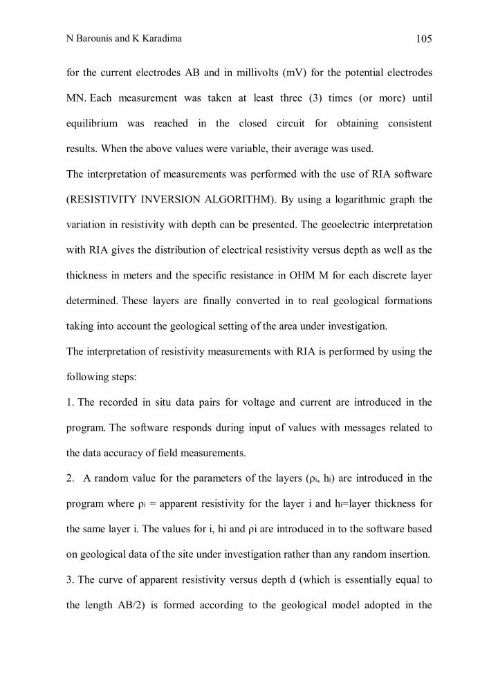
N Barounis and K Karadima 105
for the current electrodes AB and in millivolts (mV) for the potential electrodes
MN. Each measurement was taken at least three (3) times (or more) until
equilibrium was reached in the closed circuit for obtaining consistent
results. When the above values were variable, their average was used.
The interpretation of measurements was performed with the use of RIA software
(RESISTIVITY INVERSION ALGORITHM). By using a logarithmic graph the
variation in resistivity with depth can be presented. The geoelectric interpretation
with RIA gives the distribution of electrical resistivity versus depth as well as the
thickness in meters and the specific resistance in OHM M for each discrete layer
determined. These layers are finally converted in to real geological formations
taking into account the geological setting of the area under investigation.
The interpretation of resistivity measurements with RIA is performed by using the
following steps:
1. The recorded in situ data pairs for voltage and current are introduced in the
program. The software responds during input of values with messages related to
the data accuracy of field measurements.
2. A random value for the parameters of the layers (ρi, hi) are introduced in the
program where ρi = apparent resistivity for the layer i and hi=layer thickness for
the same layer i. The values for i, hi and ρi are introduced in to the software based
on geological data of the site under investigation rather than any random insertion.
3. The curve of apparent resistivity versus depth d (which is essentially equal to
the length AB/2) is formed according to the geological model adopted in the
Application of half Schlumberger configuration for… 106
previous step 2. The curve is formed by using forward calculations algorithms of
the Ghosh type (Ghosh, 1971).
4. Adjustments for the ρi and hi values with trial and error until the RIA
computational theoretical curve matches the curve for actual in situ measurements
of step 1. The theoretical curves have been calculated previously by various
researchers (Ghos, 1971; Kumar and Das, 1977; Koefoed, 1979). RIA at the fourth
step uses the method of least squares (iterative least squares procedure). The
method was introduced in 1973 by Inman (Inman, 1973) and completed in 1977
by Johansen (Johansen, 1975; Johansen, 1977).
The method of least squares is applied by using the formula:
ND
weightRhoacRhoamx
2lnln (3)
where Rhoam = apparent resistivity measured at the site (Ohm m)
Rhoac = calculated apparent resistivity from theoretical models with the aid
of RIA (Ohm m)
ND = number of measurements
The geological model is closer to the theoretical model as the value of x above
becomes smaller. A few geological models with trial and error (typically between
5 and 10) have to be tested before adopting the final one.

N Barounis and K Karadima 107
4 Results of half Schlumberger surveys
The project was consisting of 21 wind turbines. For each one, two (2) soundings
were executed with a total of 42 soundings. The investigation depth for each one
was 50 meters. The two typical configurations followed for each W/T were: 3.2, 5,
6.4, 10, 25, 32, 50m and 3.2, 6.4, 10, 16, 25, 32 and 50m. The general result after
RIA interpretations for all 42 soundings was that the geological profile consisted
of a two layered medium.
The prevailing geoelectrical condition determined was:
ρ2>ρ1
where ρ1= resistivity of first upper layer (Ohm m)
ρ2 = resistivity of second deeper layer (Ohm m).
The best average geological model that fitted all the collected data had a first
upper conductive layer (ρ1) with thickness between 0.1 and 6.5m and resistivity
between 100 and 260 Ohm m. The second layer was having a higher resistivity
(ρ2) between 613 and 5788Ohm m. The first layer was conductive enough to be
interpreted as clay (terra rosa) that has resulted from weathering of the second
deeper layer of limestone. The second layer was detected at very shallow depths
down to 6.5 meters deep from the free surface and it was interpreted as the
limestone bedrock of the site. In figures 2 and 3 are shown two typical examples
for raw data curves of soundings 5 and 6 and in figures 4 and 5 their resulting
geoelectrical and geological models after the interpretation with RIA.

Application of half Schlumberger configuration for… 108
Figure 2: Raw data curve for sounding 5 with a discrete peak at 32m depth -W/T 3
Figure 3: Raw data for sounding 6 with a discrete peak at 32m depth for -W/T 3

N Barounis and K Karadima 109
Figure 4: Resulting interpretation with RIA for raw data curve of figure 2
(ρ1=211Οhm m- h1=6.5m and ρ2=1476.2Οhm m)
Figure 5: Resulting interpretation with RIA for raw data curve of figure 3
(ρ1=255.1Οhm m- h1=3.4m and ρ2=1316.9Οhm m)
Application of half Schlumberger configuration for… 110
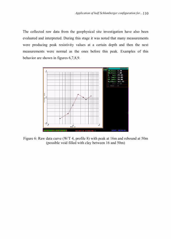
The collected raw data from the geophysical site investigation have also been
evaluated and interpreted. During this stage it was noted that many measurements
were producing peak resistivity values at a certain depth and then the next
measurements were normal as the ones before this peak. Examples of this
behavior are shown in figures 6,7,8,9.
Figure 6: Raw data curve (W/T 4, profile 8) with peak at 16m and rebound at 50m (possible void filled with clay between 16 and 50m)
N Barounis and K Karadima 111
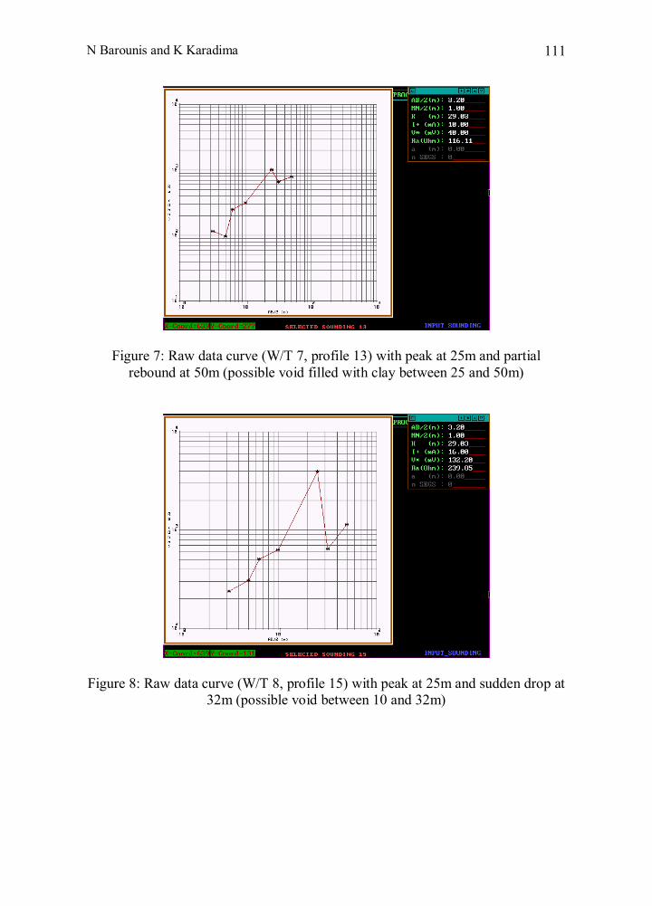
Figure 7: Raw data curve (W/T 7, profile 13) with peak at 25m and partial rebound at 50m (possible void filled with clay between 25 and 50m)
Figure 8: Raw data curve (W/T 8, profile 15) with peak at 25m and sudden drop at 32m (possible void between 10 and 32m)

Application of half Schlumberger configuration for… 112
Figure 9: Raw data curve (W/T 8, profile 16) with peak at 25m and sudden drop at 32m matching the curve in figure 9 for the same W/T
Figure 10: Raw data curve (W/T 9, profile 18) with sudden drop at 25m and rebound at 32m (possible void filled with clay between 16 and 32m)

N Barounis and K Karadima 113
Figure 11: Raw data curve (W/T 15, profile 30) with sudden drop at 25m and rebound at 32m (possible void filled with clay between 16 and 32m)
Figure 12: Raw data curve (W/T 18, profile 36) with sudden drop at 16m, peak at 25m and drop at 32m (possible void filled with clay between 10 and 16m and
karstic void between 16 and 32m)

Application of half Schlumberger configuration for… 114
Figure 13: Raw data curve (W/T 21, profile 42) with sudden drop at 25 and rebound at 50m (possible void filled with clay between 16 and 50m)
The important information was revealed not only from the interpretation of the
measurements, but from the raw curves. It is evident from the pattern of these
curves shown above that these peaks or sudden drops could be associated with the
presence of cavities of karstic origin. This sounded very heretic because it is very
rare the case for karstic voids in Triassic and Cretaceous Limestone at the top of a
mountain which is badly sheared, faulted and folded and at the same time there are
no signs of karstic processes on the ground surface. The suspicions were stronger
when one observes that the raw curves present very sudden resistivity decreases
and after a few measurements the resistivity increases abruptly by taking into
account the 1900m altitude and the massive limestone thickness. This could be
associated with the presence of karstic voids that has been filled with clay (tera
rosa) from the weathering of limestone and water action. Below the void the
limestone is intact and compared to the filled with clay void, it has greater
resistivity. Thus the resistivity increases again as the electrodes are further
deployed.
The half Schlumberger configuration thus proved to be sensitive enough for
locating probable void locations or voids that have been filled with some form of

N Barounis and K Karadima 115
conductive material like clay.
5 Conclusions Geophysical site investigation was applied at a very early stage for the
construction of a wind farm at Central Continental Greece. The wind farm was
consisting of 21 wind turbines developing on the crest of a mountain. The site was
mainly consisted of massive limestone and the scope of the geophysical survey
was to detect the presence of voids or filled cavities that could put in risk the
project.
The half Schlumberger configuration was proposed for detecting such voids and it
proved to be efficient. The sensitivity of half Schlumberger configuration could be
attributed to the interval between successive measurements. In contrast to
Schlumberger, Wenner configuration collects data usually every meter and thus
the raw data curve it is continuous between 1 and 50 meters. The discontinuity of
half Schlumberger configuration (for example from 16m to 25m depth leaves a
gap of 9m) gives a better pronounce to the peaks and drops of resistivity. But on
the other hand the collected data leave a big gap between the upper and the lower
elevation of the probable void.
A detected void between 16 and 50m depth for example (W/T 21, profile 42) can
be of no engineering use since such a void could impose a high risk with its exact
dimensions unknown. Optimization of the site investigation can be achieved only
by applying direct methods like drilling boreholes and sampling at the suspect
locations (hot spots) beneath the wind turbines. In this way the interpretation with
half Schlumberger configuration becomes a tool for designing the next step of the
site investigation scheme by executing boreholes and in situ testing. In this way
qualitative and quantitative methods are linked with resulting reduction for the site
investigation cost from deep boreholes. Such boreholes could also prove to be
unnecessary when direct methods are only used without applying geophysical
investigations at an earlier stage.

Application of half Schlumberger configuration for… 116
References [1] Arabelos, D. (1991). Elements of geophysical soundings. Ziti Editions,
Salonica.
[2] Beck, A. (1991). Physical principles of exploration methods. Wuerz
Publishing , Canada.
[3] Kearey, P. and Brooks, M. (1994). An introduction to geophysical
Exploration. Blackwell Scientific, Oxford.
[4] Parasnis, D. (1967) Principles of applied geophysics. Methuen, USA.
[5] Legget, F.R. and Hatheway A. W. (1988). Geology and engineering.
McGraw-Hill international editions.
[6] Reynolds, J. M. (1997). An introduction to applied and environmental
geophysics. John Wiley and Sons, England.
[7] Dobrin, M. B. and Savit C. H. (1988). Geophysical prospecting.
McGraw-Hill international editions.
[8] Simons, N. Menzies, B. Matthews, M. (2002). Geotechnical site investigation.
Thomas Telford editions, England.
[9] Sharma, P. V. (1997). Environmental and engineering geophysics.
Cambridge University Press, England.
[10] Johansen, H.K. (1975). An interactive computer/graphic display-terminal
system for interpretation of resistivity soundings. Geophysical prospecting 23,
pp. 449-458.
[11] Johansen, H.K. (1977). A man/computer interpretation system for resistivity
soundings over a horizontally stratified earth. Geophysical prospecting 25, pp.
667-691.