G.J. E.D.T., Vol. 1(2) 2012:19-31 ISSN 2319 – 7293

19

APPLICATION OF HEC HMS/RAS AND GIS TOOLS IN FLOOD MODELING: A CASE STUDY FOR RIVER SIRONKO – UGANDA.

Okirya Martin1, Albert Rugumayo2 & Janka Ovcharovichova3 1Department of Agricultural Mechanization and Irrigation Engineering, Busitema University, Kampala – Uganda

2Department of Civil and Environmental Engineering, School of Engineering, College Of Engineering Design Art And Technology,

Makerere University, Kampala – Uganda 3Council for Frontiers of Knowledge (CFK), 2 Oakwood Court, Camp Hill, Pennsylvania, 17011 - 1547, USA,

Abstract

Hydrological modeling was performed using HEC HMS software, after delineating the catchment basin model (325

km2) using HEC GeoHMS in ArcGIS environment, populating the meteorological model with design storm data, and

defining control specifications. The 10, 50, 100, 250, and 500 year design storms data input into the model generated

design floods of 71.8 m3/s, 123.0 m

3/s, 138.5 m

3/s, 163.9 m

3/s, and 183.4 m

3/s magnitudes respectively. Hydraulic

modeling was performed using HEC RAS software. The model output channel flood depths at the gauging station were

5.21m, 6.53m, 6.84m, 7.31m, and 7.65m for simulated 10, 50, 100, 250, and 500 year design floods respectively. Flood

hazard maps were generated by exporting the HEC RAS model output results to ArcGIS where they were processed to

identify the flood prone areas. From the flood hazard maps, the most flood prone areas were around the river middle

reach.

Key Words: GIS; Flood modeling; HEC – HMS/RAS; HEC – GeoHMS/RAS

1. Introduction

Globally floods are increasingly among the most devastating natural disasters affecting human life than any other

natural disasters. According to Abhas, Jha, and Jessica (2012), in 2010 alone, 178 million people were affected by floods

and the total financial losses in the exceptional years such as 1998 and 2010 exceeded $40 billion. It is also reported that

one sixth of the global population (one billion people); the majority of them among the world's being low income earners

live in the potential path of a 1 in 100 year flood according to Department for International Development (DFID).

Uganda is facing the same global challenges of extreme climate change effects of droughts and floods. Most floods in

Uganda are due to torrential storms that result in bursting of river banks and thereby cause floods. Uganda receives

between 900mm and 2000mm of rainfall annually according to Uganda National Water Development (UNWD) (2005)

report, with the highest annual rainfall being experienced around the slopes of Mt Elgon. Sironko district stretches to the

slopes of Mt Elgon which experiences high amounts of rainfall annually. In 2007, several districts in Uganda such as

Lira, Amuria, Katakwi, Bukedea, Kumi and Soroti were affected by floods with the worst hit being Katakwi and Amuria in Teso region. The floods destroyed roads, overtopped and washed away bridges and roads, rendering some areas

inaccessible according to reports. There was severe outbreak of starvation among the displaced population and fear of

outbreak of water-borne diseases. Again in 2011, Sironko and the neighbouring Eastern districts, experienced floods

from torrential rains and bursting of river banks that left many homeless, damaged property and affected area of about

37846.35 km2

(Dartmouth Flood Observatory (DFO), 2011). Water related disasters in Uganda such as droughts, floods,

landslides, windstorms and hailstorms contribute well over 70% of the natural disasters and destroy annually an average

of 800,000 hectares of crops making economic losses in excess of 120 billion shillings (UNWD, 2005). The recent floods

in Sironko district is reported to have destroyed property, field crops, livestock, bridges and roads, water sources, among

others (DFO, 2011).

Flood modeling can easily be accomplished using the readily available tools such as HEC HMS/RAS and GIS tools.

When calibrated well, the results of the models offer a reliable tool to be used in decision making by the district and

national policy makers in the country. In both rural and urban establishments of Uganda, many flood plains and wetlands

have been used extensively for agricultural production, sand mining, and major building construction projects. This is

partly because many river flood plains in the country have not yet been delineated. HEC RAS/HMS tools have been

tested and widely used globally in flood modeling for several years (Maidment & Seth, 1999).

1.1 Research goals

The main goal of the research was to develop flood hazard maps from which the flood prone areas within the district

would be identified. The specific goals of the research included the following:

1. Perform rainfall – runoff analysis (hydrological modeling) for river Sironko basin.

2. Perform hydraulic modeling for river Sironko

3. Prepare flood hazard maps for Sironko district.

1.2 Research motivation

G.J. E.D.T., Vol. 1(2) 2012:19-31 ISSN 2319 – 7293

20

Floods are associated with massive destruction of field crops, property and ultimately food insecurity. From the

Central intelligence Agency (CIA) World Fact book website, the 2012 estimate of Uganda’s annual population growth is

3.3%, a clear indication that the nation’s population is increasing at a high rate. Increased population growth among other

things leads to increased urbanization, over exploitation of natural resources such as agricultural lands, forests, wetlands,

and water bodies. Flood hazard maps are key tools that can be used in decision making when developing policies for land

use and management of flood plains. In addition to this, district farmers can plan and choose wisely which crops to be

grown in flood prone areas so as to minimize field crop losses associated with floods thereby ensuring food security in

the district and country.

1.3 Paper overview

The subsequent sections of this paper include; (a) Description of datasets section; (b) the methodological section

which describes the study area, datasets used, hydrological modeling, hydraulic modeling, and flood hazard map

generation; (c) results and discussion section which contains a presentation of model results, flood hazard maps and

discussions; (d) the conclusion and recommendation section; (e) challenges encountered; (f) acknowledgements; and (g)

references.

2. Description of datasets used

2.1 Hydrologic modeling datasets

Digital Elevation Model (DEM)

The DEM was a fundamental dataset used for development of the basin model component in the HEC HMS model

and the geometrical data model in the HEC RAS model. This dataset was therefore useful in hydrological modeling,

hydraulic modeling, and flood hazard map generation. The DEM used was of cell size 92.52 m by 92.52 m.

Land use/cover shape files

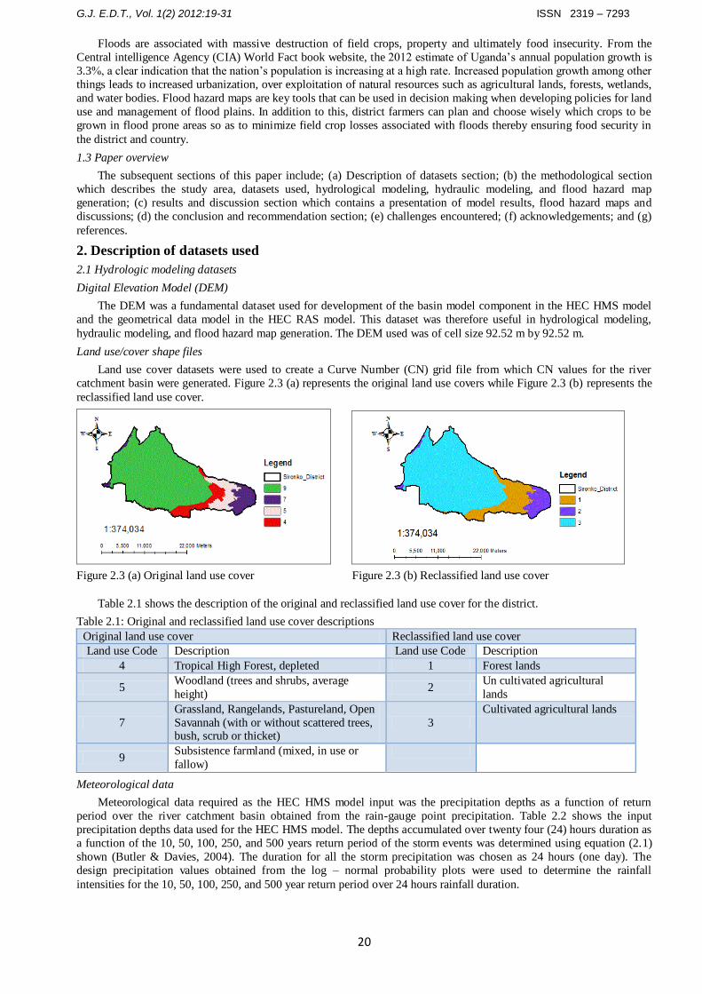
Land use cover datasets were used to create a Curve Number (CN) grid file from which CN values for the river

catchment basin were generated. Figure 2.3 (a) represents the original land use covers while Figure 2.3 (b) represents the

reclassified land use cover.

Figure 2.3 (a) Original land use cover Figure 2.3 (b) Reclassified land use cover

Table 2.1 shows the description of the original and reclassified land use cover for the district.

Table 2.1: Original and reclassified land use cover descriptions

Original land use cover Reclassified land use cover

Land use Code Description Land use Code Description

4 Tropical High Forest, depleted 1 Forest lands

5 Woodland (trees and shrubs, average

height) 2

Un cultivated agricultural

lands

7

Grassland, Rangelands, Pastureland, Open

Savannah (with or without scattered trees, bush, scrub or thicket)

3

Cultivated agricultural lands

9 Subsistence farmland (mixed, in use or

fallow)

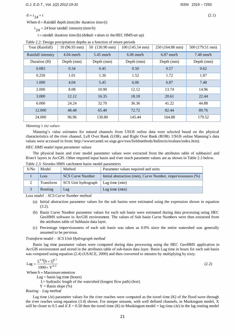
Meteorological data

Meteorological data required as the HEC HMS model input was the precipitation depths as a function of return

period over the river catchment basin obtained from the rain-gauge point precipitation. Table 2.2 shows the input

precipitation depths data used for the HEC HMS model. The depths accumulated over twenty four (24) hours duration as

a function of the 10, 50, 100, 250, and 500 years return period of the storm events was determined using equation (2.1)

shown (Butler & Davies, 2004). The duration for all the storm precipitation was chosen as 24 hours (one day). The

design precipitation values obtained from the log – normal probability plots were used to determine the rainfall

intensities for the 10, 50, 100, 250, and 500 year return period over 24 hours rainfall duration.

G.J. E.D.T., Vol. 1(2) 2012:19-31 ISSN 2319 – 7293

21

up)set HMS HEC in the alues(default v (h) imeduration t rainfall t

(mm/h)intensity rainfallhour 24 24

i

(t) imeduration tfor (mm)depth Rainfall d Where

(2.1) t 24

id

Table 2.2: Design precipitation depths as a function of return periods

Year (Rainfall) 10 (96.93 mm) 50 (130.90 mm) 100 (145.54 mm) 250 (164.88 mm) 500 (179.51 mm)

Rainfall intensity 4.04 mm/h 5.45 mm/h 6.06 mm/h 6.87 mm/h 7.48 mm/h

Duration (H) Depth (mm) Depth (mm) Depth (mm) Depth (mm) Depth (mm)

0.083 0.34 0.45 0.50 0.57 0.62

0.250 1.01 1.36 1.52 1.72 1.87

1.000 4.04 5.45 6.06 6.87 7.48

2.000 8.08 10.90 12.12 13.74 14.96

3.000 12.12 16.35 18.18 20.61 22.44

6.000 24.24 32.70 36.36 41.22 44.88

12.000 48.48 65.40 72.72 82.44 89.76

24.000 96.96 130.80 145.44 164.88 179.52

Manning’s (n) values

Manning’s value estimates for natural channels from USGS online data were selected based on the physical

characteristics of the river channel, Left Over Bank (LOB), and Right Over Bank (ROB). USGS online Manning’s data

values were accessed in from: http://wwwrcamnl.wr.usgs.gov/sws/fieldmethods/Indirects/nvalues/index.htm).

HEC HMS model input parameter values

The physical basin and river model parameter values were extracted from the attributes table of subbasin1 and

River1 layers in ArcGIS. Other required input basin and river reach parameter values are as shown in Table 2.3 below.

Table 2.3: Sironko HMS catchment basin model parameters

S/No Model Method Parameter values required and units

1 Loss SCS Curve Number Initial abstraction (mm), Curve Number, imperviousness (%)

2 Transform SCS Unit hydrograph Lag time (min)

3 Routing Lag Lag time (min)

Loss model – SCS Curve Number method

(a) Initial abstraction parameter values for the sub basins were estimated using the expression shown in equation

(3.2).

(b) Basin Curve Number parameter values for each sub basin were estimated during data processing using HEC

GeoHMS software in ArcGIS environment. The values of Sub basin Curve Numbers were then extracted from

the attributes table of Subbasin data layer.

(c) Percentage imperviousness of each sub basin was taken as 0.0% since the entire watershed was generally

assumed to be pervious.

Transform model – SCS Unit Hydrograph method

Basin lag time parameter values were computed during data processing using the HEC GeoHMS application in

ArcGIS environment and stored in the attributes table of sub-basin data layer. Basin Lag time in hours for each sub basin

was computed using equation (2.4) (USACE, 2000) and then converted to minutes by multiplying by sixty.

retention Maximum S Where

(2.2) Y1900

1SLLag

0.5

0.70.8

Lag = basin lag time (hours)

L= hydraulic length of the watershed (longest flow path) (feet)

Y = Basin slope (%)

Routing – Lag method

Lag time (∆t) parameter values for the river reaches were computed as the travel time (K) of the flood wave through

the river reaches using equation (3.4) shown. For steeper streams, with well defined channels, in Muskingum model, X will be closer to 0.5 and if X = 0.50 then the travel time (K) in Muskingum model = lag time (∆t) in the lag routing model

G.J. E.D.T., Vol. 1(2) 2012:19-31 ISSN 2319 – 7293

22

(USACE, 2000). In Muskingum model, X is the dimensionless weight factor ranging between 0.0 and 0.5 (0.0 for a

linear reservoir, 0.5 for a pure transmission reach).

The travel time K of the flood wave was estimated using equation (2.3) expressed below:

(2.3) V

LK

Where L = Length of the river reaches (m). River reach lengths were created after processing Sironko_DEM and stored

in the river layer attributes table.

V = Velocity of the flood wave through the reach (m/s) was obtained using equation (2.4)

(2.4) A

QV

Where Q = flood discharge at the gauging station (m3/s)

A = Cross section area at the gauging station (m2).

The Muskingum routing model is as shown in equation (2.5) (USACE, 2000).

(2.5) QΔtX-12K

ΔXX-12kI

ΔtX12K

2KXΔtI

ΔtX12K

2KXΔtQ 1t1tt(t)

Where Q(t) = outflow from storage at time t (cfs)

∆t = time increment (h)

K= Travel time of the flood wave in the reach (h)

X = dimensionless weight ranging between 0.0 and 0.5 (0.0 for a linear reservoir, 0.5 for a pure transmission

reach).

I (t) = average inflow to storage at time t (cfs)

Qt-1 = outflow from storage at previous time t-1(cfs)

Table 2.4: Loss and Transform model parameter value estimates

Basin ID

(1)

Basin Areas

(Km2) (2)

Basin CN

(3)

S

(4)

Ia (inches)

(5)

Ia (mm)

(6)

Basin CN*

(7)

Basin Lag (min)

(8)

W 340 28.258 68 4.67 0.93 23.70 61 3129

W 330 26.906 70 4.29 0.86 21.78 63 1650

W 320 23.259 75 3.38 0.68 17.19 67 938

W 300 16.856 72 3.86 0.77 19.59 65 1195

W 290 23.156 69 4.39 0.88 22.30 63 1713

W 280 20.614 81 2.38 0.48 12.08 73 797

W 270 16.761 80 2.53 0.51 12.84 72 771

W 260 11.950 81 2.35 0.47 11.92 73 796

W 250 33.668 81 2.35 0.47 11.92 73 1460

W 240 13.671 81 2.35 0.47 11.92 73 798

W 230 34.131 81 2.35 0.47 11.92 73 1332

W 220 22.326 81 2.35 0.47 11.92 73 938

W 200 38.668 81 2.35 0.47 11.92 73 1721

W 190 14.844 81 2.35 0.47 11.92 73 912

Basin CN* (The Curve Number parameter values in column (7) have been calibrated by reducing the original Curve Number values in

column (3) by 10 %.)

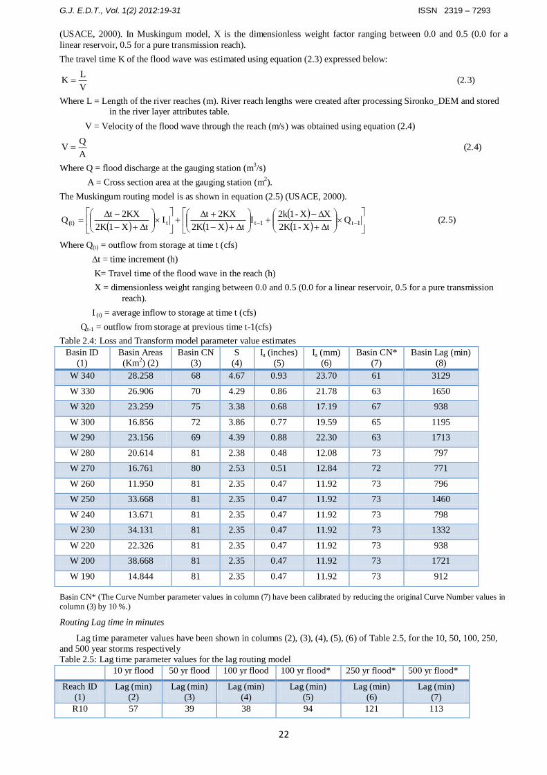
Routing Lag time in minutes

Lag time parameter values have been shown in columns (2), (3), (4), (5), (6) of Table 2.5, for the 10, 50, 100, 250,

and 500 year storms respectively

Table 2.5: Lag time parameter values for the lag routing model

10 yr flood 50 yr flood 100 yr flood 100 yr flood* 250 yr flood* 500 yr flood*

Reach ID

(1)

Lag (min)

(2)

Lag (min)

(3)

Lag (min)

(4)

Lag (min)

(5)

Lag (min)

(6)

Lag (min)

(7)

R10 57 39 38 94 121 113

G.J. E.D.T., Vol. 1(2) 2012:19-31 ISSN 2319 – 7293

23

R20 54 37 35 89 114 106

R50 26 18 17 43 55 51

R60* 191 132 125 313 400 375

R80 192 132 126 316 404 379

R110 66 45 44 109 139 131

R130 52 36 34 86 110 103

R150 28 19 18 46 59 55

R60*(This is an upper tributary contributing smaller amounts of flow to the river. Its velocity of flow has be considered as a third of the general flow velocities)

250 year flood*(To obtain the lag time for 250 year storm, the lag time for 1 100 year storm was multiplied by 3.2.)

500 year flood*(To obtain the lag time for 500 year storm, the lag time for 1 100 year storm was multiplied by 3.)

100 year flood*(The calculated lag time parameters were calibrated by multiplying the original lag time values by 2.5 which resulted into an error 0.13 %.)

2.2 Hydraulic model datasets

Geometrical model datasets required for hydraulic modeling included the following;

1. River name, reach name, river cross section station, downstream reach lengths (LOB, channel, ROB), main channel

bank stations. These were all created during data processing using HEC GeoRAS in ArcGIS and then imported to HEC

RAS model geometrical editor where they were edited based on field survey data.

2. Manning’s n values. Manning’s value estimates for natural channels from USGS online data were selected based on

the physical characteristics of the channel, Left Over Bank (LOB), and Right Over Bank (ROB). USGS online

Manning’s data values were accessed in April 2012 from:

http://wwwrcamnl.wr.usgs.gov/sws/fieldmethods/Indirects/nvalues/index.htm).

3. Contraction and expansion default coefficient parameter values for steady flow regime were automatically assigned by

HEC RAS program.

4. Bridge data. The bridge data included the following: Distance (Upstream bridge distance – obtained from field survey

measurements) (ft), bridge width in the direction of flow (ft) (this was also obtained from field survey measurements),

weir coefficient (default value was accepted), high Chord elevation value (ft) (obtained from the cross section

elevation data), low Chord elevation value (ft) (obtained from the cross section elevation data), vertical walls (opening

width – checked the box Add Vertical Walls in Deck from the bridge design editor tab window) (ft), and Sloping abutments (side slope horizontal value). These were estimated from field survey data obtained.

Steady flow datasets

The steady flow input data for Sironko RAS model was created from Sironko HMS model. The Sironko HMS model

flow data output for 10, 50, 100, 250, and 500 year return period were the input steady flow data for the upper tributary,

lower tributary, upper reach, middle reach, and lower reach river reaches respectively.

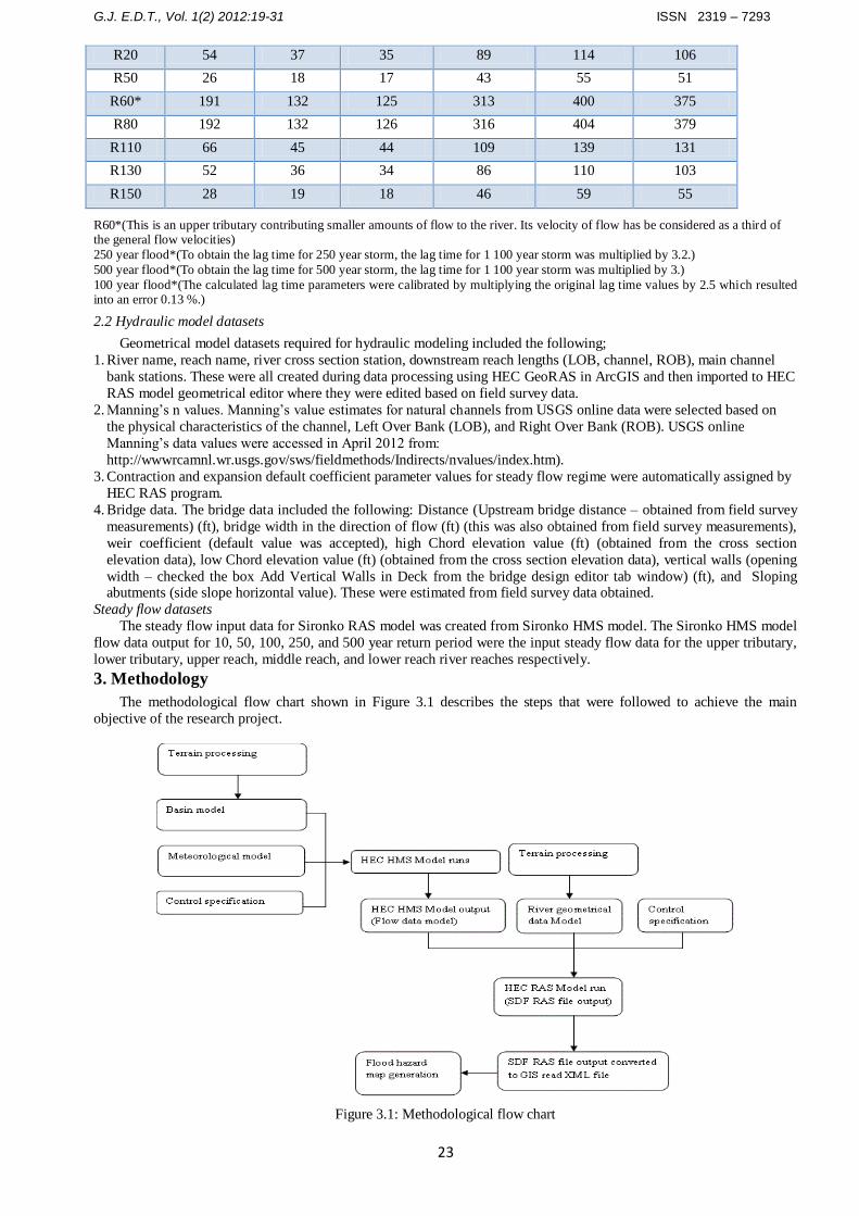
3. Methodology

The methodological flow chart shown in Figure 3.1 describes the steps that were followed to achieve the main

objective of the research project.

Figure 3.1: Methodological flow chart

G.J. E.D.T., Vol. 1(2) 2012:19-31 ISSN 2319 – 7293

24

Terrain processing steps

Terrain processing involved the following steps; 1. Fill Sinks, 2. Flow Direction, 3. Flow Accumulation, 4. Stream

Definition, 5. Stream Segmentation, 6. Catchment Grid Delineation, 7. Catchment Polygon Processing, 8. Drainage

Line Processing, 9. Adjoint Catchment Processing performed in sequential order

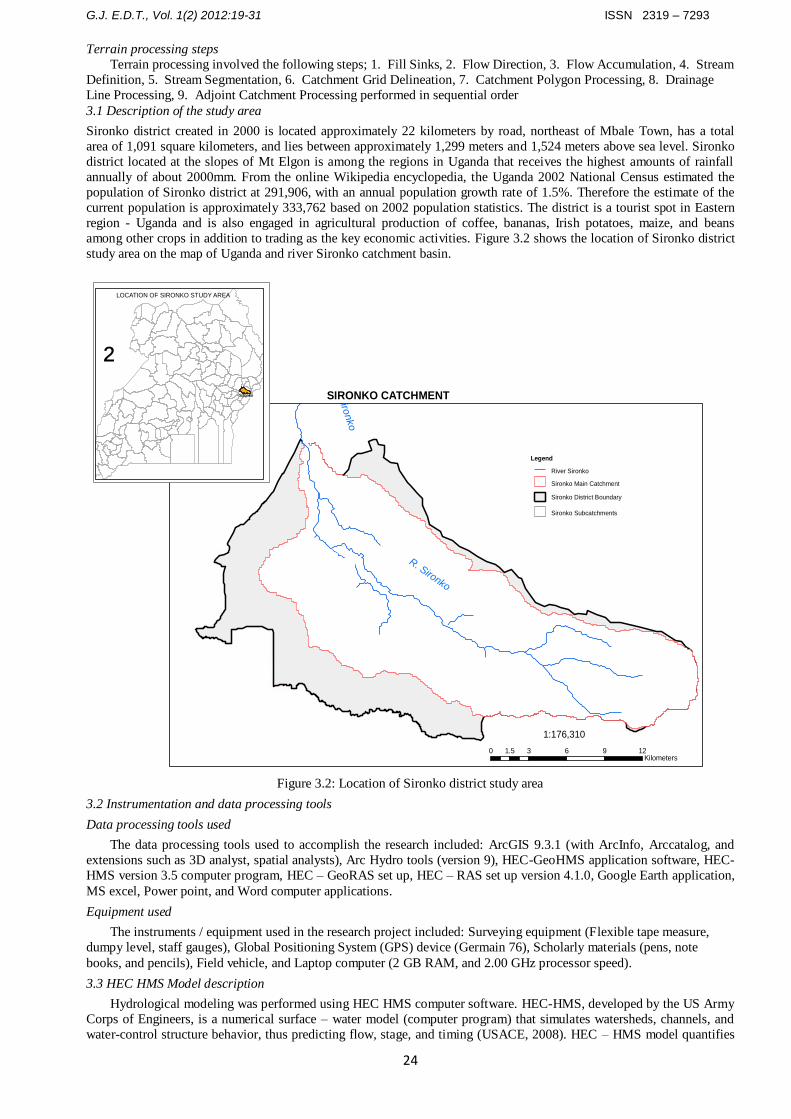
3.1 Description of the study area

Sironko district created in 2000 is located approximately 22 kilometers by road, northeast of Mbale Town, has a total

area of 1,091 square kilometers, and lies between approximately 1,299 meters and 1,524 meters above sea level. Sironko

district located at the slopes of Mt Elgon is among the regions in Uganda that receives the highest amounts of rainfall

annually of about 2000mm. From the online Wikipedia encyclopedia, the Uganda 2002 National Census estimated the

population of Sironko district at 291,906, with an annual population growth rate of 1.5%. Therefore the estimate of the

current population is approximately 333,762 based on 2002 population statistics. The district is a tourist spot in Eastern

region - Uganda and is also engaged in agricultural production of coffee, bananas, Irish potatoes, maize, and beans

among other crops in addition to trading as the key economic activities. Figure 3.2 shows the location of Sironko district

study area on the map of Uganda and river Sironko catchment basin.

R. Sironko

R. S

ironko

Sironko

LOCATION OF SIRONKO STUDY AREA

SIRONKO CATCHMENT

²

0 3 6 9 121.5Kilometers

1:176,310

Legend

River Sironko

Sironko Main Catchment

Sironko District Boundary

Sironko Subcatchments

Figure 3.2: Location of Sironko district study area

3.2 Instrumentation and data processing tools

Data processing tools used

The data processing tools used to accomplish the research included: ArcGIS 9.3.1 (with ArcInfo, Arccatalog, and

extensions such as 3D analyst, spatial analysts), Arc Hydro tools (version 9), HEC-GeoHMS application software, HEC-

HMS version 3.5 computer program, HEC – GeoRAS set up, HEC – RAS set up version 4.1.0, Google Earth application,

MS excel, Power point, and Word computer applications.

Equipment used

The instruments / equipment used in the research project included: Surveying equipment (Flexible tape measure,

dumpy level, staff gauges), Global Positioning System (GPS) device (Germain 76), Scholarly materials (pens, note

books, and pencils), Field vehicle, and Laptop computer (2 GB RAM, and 2.00 GHz processor speed).

3.3 HEC HMS Model description

Hydrological modeling was performed using HEC HMS computer software. HEC-HMS, developed by the US Army

Corps of Engineers, is a numerical surface – water model (computer program) that simulates watersheds, channels, and

water-control structure behavior, thus predicting flow, stage, and timing (USACE, 2008). HEC – HMS model quantifies

G.J. E.D.T., Vol. 1(2) 2012:19-31 ISSN 2319 – 7293

25

rainfall losses into the soil and converts excess rainfall to runoff, and routing (Maidment & Seth, 1999). HEC HMS has

three major components i.e. (a) the basin model component containing information related to the physical attributes of

the basin, such as areas, river reach connectivity and length; (b) the precipitation model that hold precipitation data input

files and (c) control specifications section that contains information pertinent to the timing of the model such as when a

storm occurred and what type of time interval one wants to use in the model. The empirical models that define the

partitioning of rainfall into infiltration and runoff are as shown in equations (3.1), (3.2), and (3.3) (USACE, 2000);

(3.3) 10CN

1000S

(3.2) 0.2SI

(3.1) 0.8SP

0.2S-PQ

a

2

Where, Q = runoff (in)

P = rainfall (in)

S = potential maximum retention

Ia = initial abstraction (in)

CN = runoff Curve Number value

3.4 Hydrological modeling

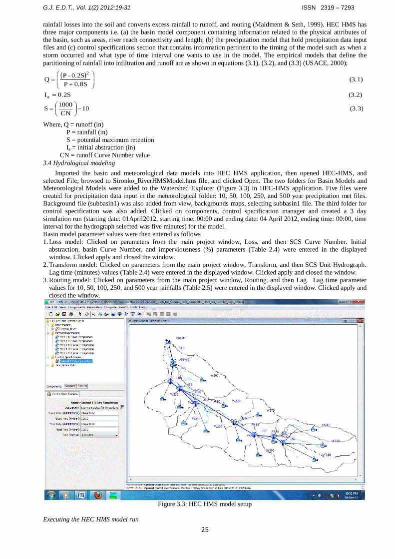
Imported the basin and meteorological data models into HEC HMS application, then opened HEC-HMS, and

selected File; browsed to Sironko_RiverHMSModel.hms file, and clicked Open. The two folders for Basin Models and Meteorological Models were added to the Watershed Explorer (Figure 3.3) in HEC-HMS application. Five files were

created for precipitation data input in the meteorological folder: 10, 50, 100, 250, and 500 year precipitation met files.

Background file (subbasin1) was also added from view, backgrounds maps, selecting subbasin1 file. The third folder for

control specification was also added. Clicked on components, control specification manager and created a 3 day

simulation run (starting date: 01April2012, starting time: 00:00 and ending date: 04 April 2012, ending time: 00:00, time

interval for the hydrograph selected was five minutes) for the model.

Basin model parameter values were then entered as follows

1. Loss model: Clicked on parameters from the main project window, Loss, and then SCS Curve Number. Initial

abstraction, basin Curve Number, and imperviousness (%) parameters (Table 2.4) were entered in the displayed

window. Clicked apply and closed the window.

2. Transform model: Clicked on parameters from the main project window, Transform, and then SCS Unit Hydrograph.

Lag time (minutes) values (Table 2.4) were entered in the displayed window. Clicked apply and closed the window.

3. Routing model: Clicked on parameters from the main project window, Routing, and then Lag. Lag time parameter

values for 10, 50, 100, 250, and 500 year rainfalls (Table 2.5) were entered in the displayed window. Clicked apply and

closed the window.

Figure 3.3: HEC HMS model setup

Executing the HEC HMS model run

G.J. E.D.T., Vol. 1(2) 2012:19-31 ISSN 2319 – 7293

26

Selected compute from the main project window menu and then created simulation runs for 10, 50, 100, 250, and

250 year floods from the run manager. Changed default names of the runs (Run 1, 2, 3, 4, and 5) to Run 110 year flood,

Run 2 50 year flood, Run 3 100 year, Run 4 250, and Run 5 500 year flood, clicked next to complete all the steps and

finally clicked finish to complete creating the runs one after the other. To run the model, selected compute, Select run,

and then computed the 10, 50, 100, 250, and 500 year floods by clicking the compute tab.

3.5 HEC – RAS model description

HEC-RAS, developed by the US Army Corps of Engineers, is a one-dimensional steady flow hydraulic model

designed to aid hydraulic engineers in channel flow analysis and floodplain delineation (USACE, 2010). HEC RAS has

three main components: - (a) the geometry data which consists of a description of the size, shape, and connectivity of

stream cross-sections; (b) the Flow data which contains discharge rates; and (c) the Plan data which contains information

pertinent to the run specifications of the model, such as a description of the flow regime. The primary procedure used by

HEC-RAS to compute water surface profiles assumes a steady, gradually varied flow scenario. The basic computational

procedure is based on an iterative solution of the energy equation (3.4) shown (Butler & Davies, 2004).

(3.4) 2g

V

ρg

PZH

2

Where H = Total Energy Head (m)

Z = Potential head (m)

p/ρg = Pressure head (m)

P = pressure (N/m2)

ρg = Unit weight (N/m3)

V2/2g = Kinetic (velocity) head (m)

V = Velocity of flow (m/s)

g = Acceleration due to gravity (m/s2)

3.6 Hydraulic modeling

Hydraulic modeling was performed using HEC RAS software. The model set up comprised of three components; (a)

Geometry data, (b) Flow data, and (c) Plan (control specification) data.

Importing Sironko river geometry data into HEC-RAS model

Launched HEC-RAS by double clicking on HEC-RAS 4.1.0 on the desktop; then saved the new project by going to

File, Save Project as Sironko River Flood Study.prj in the working folder, clicked OK.

Importing GIS data: To import the GIS data into HEC-RAS; went to geometric data editor by clicking on Edit,

Geometric Data. In the geometric data editor, clicked on File, Import Geometry Data, GIS Format. Browsed to

GIS2RASImport.sdf file created in ArcGIS, and clicked OK. The import process asked for some inputs to complete. In

the Intro tab, confirmed SI (Metric) Units (this converted the SI metric units to US customary units) for Import data and

clicked next. Confirmed the River/Reach data, made sure all import stream lines boxes are checked, and clicked next. Confirmed cross-sections data, made sure all Import data boxes are checked for cross-sections, and clicked OK (accepted

default values for matching tolerance, round places, etc) and, clicked Finished-Import data. The data was then imported

to the HEC-RAS geometric editor. Saved the geometry file as RiverSironko_Geometry by clicking File, and the Saved

Geometry Data.

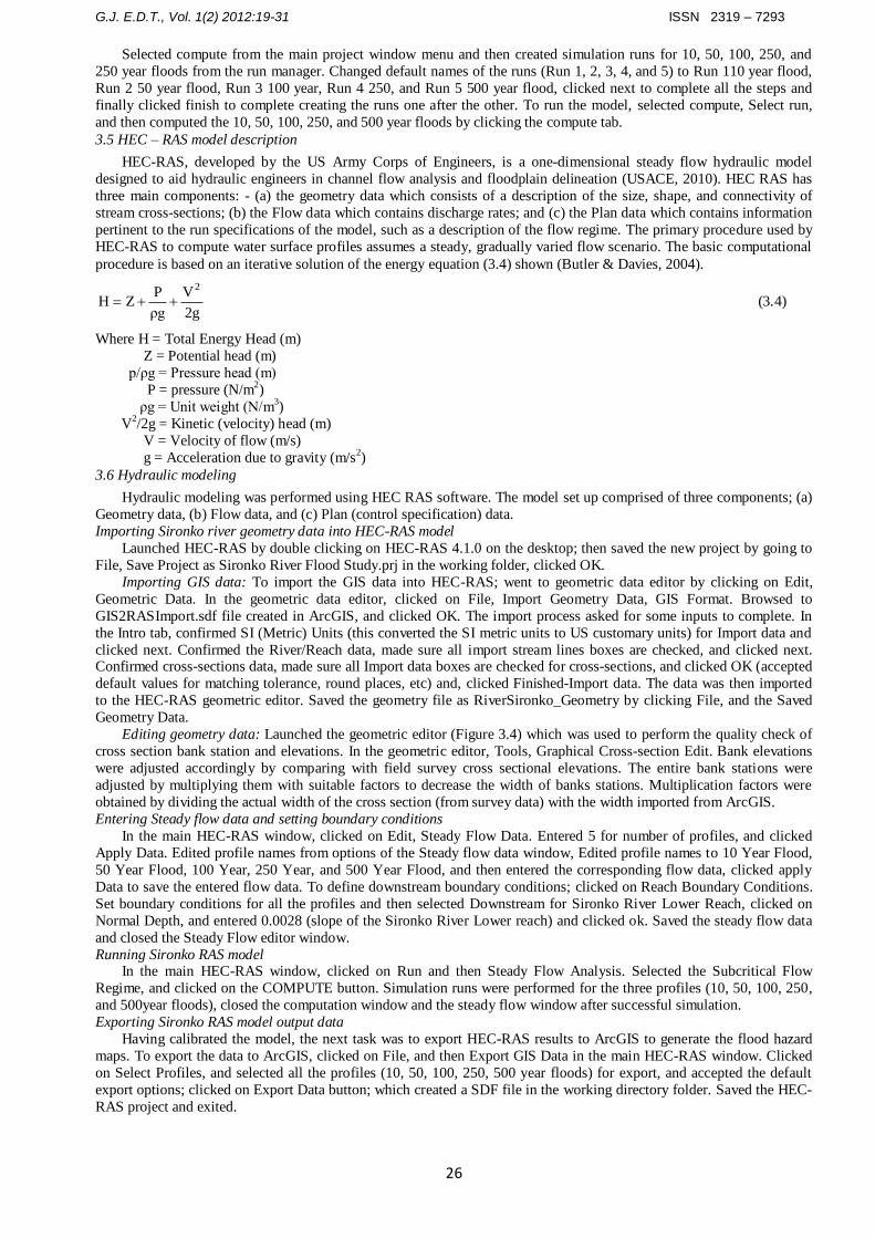
Editing geometry data: Launched the geometric editor (Figure 3.4) which was used to perform the quality check of

cross section bank station and elevations. In the geometric editor, Tools, Graphical Cross-section Edit. Bank elevations

were adjusted accordingly by comparing with field survey cross sectional elevations. The entire bank stations were

adjusted by multiplying them with suitable factors to decrease the width of banks stations. Multiplication factors were

obtained by dividing the actual width of the cross section (from survey data) with the width imported from ArcGIS.

Entering Steady flow data and setting boundary conditions

In the main HEC-RAS window, clicked on Edit, Steady Flow Data. Entered 5 for number of profiles, and clicked

Apply Data. Edited profile names from options of the Steady flow data window, Edited profile names to 10 Year Flood,

50 Year Flood, 100 Year, 250 Year, and 500 Year Flood, and then entered the corresponding flow data, clicked apply

Data to save the entered flow data. To define downstream boundary conditions; clicked on Reach Boundary Conditions.

Set boundary conditions for all the profiles and then selected Downstream for Sironko River Lower Reach, clicked on

Normal Depth, and entered 0.0028 (slope of the Sironko River Lower reach) and clicked ok. Saved the steady flow data

and closed the Steady Flow editor window.

Running Sironko RAS model In the main HEC-RAS window, clicked on Run and then Steady Flow Analysis. Selected the Subcritical Flow

Regime, and clicked on the COMPUTE button. Simulation runs were performed for the three profiles (10, 50, 100, 250,

and 500year floods), closed the computation window and the steady flow window after successful simulation.

Exporting Sironko RAS model output data

Having calibrated the model, the next task was to export HEC-RAS results to ArcGIS to generate the flood hazard

maps. To export the data to ArcGIS, clicked on File, and then Export GIS Data in the main HEC-RAS window. Clicked

on Select Profiles, and selected all the profiles (10, 50, 100, 250, 500 year floods) for export, and accepted the default

export options; clicked on Export Data button; which created a SDF file in the working directory folder. Saved the HEC-

RAS project and exited.

G.J. E.D.T., Vol. 1(2) 2012:19-31 ISSN 2319 – 7293

27

Figure 3.4: Geometrical data model setup

3.7 Flood hazard map generation

Flood hazard maps for the 10, 50, 100, 250, and 500 year floods were generated following the procedure described

in the following steps:

1. In ArcGIS (ArcMap) opened sironkogeoras file and clicked on Import RAS SDF file button to convert the SDF file

into an XML file. In the Convert RAS Output File to XML window, browsed to 10_500 SteadyFlow. RASexport.sdf,

and clicked OK. The XML file was saved with the input file name in the same folder with an xml extension.

2. Next, clicked on RAS Mapping and then Layer Setup to open the post processing layer menu; in the layer setup for

post-processing, selected the New Analysis option, and named the new analysis as Steady_Flows. Browsed to 10_500

SteadyFlow. RASexport.xml for RAS GIS Export File. Selected the Single Terrain Type, and browsed to Sironko_DEM grid. Browsed to the working folder for Output Directory; HEC-GeoRAS created a geodatabase with

the same analysis name (Steady_Flows) in the output directory. Accepted the default 93 map units for Rasterization

Cell Size; clicked OK. A new map (data frame) with the analysis name (Steady_Flow) was added to ArcMap with the

terrain data. At this stage the terrain GRID (Sironko_DEM grid) was also converted to a Digital Elevation Model

(DEM) and saved in the working folder.

3. Next clicked on RAS Mapping, Import RAS data; this created a bounding polygon, which defined the analysis extent

for inundation mapping, by connecting the endpoints of XS Cut Lines. After the analysis extent was defined, clicked

on RAS Mapping, Inundation Mapping, and then Water Surface Generation. Selected all the profiles and clicked OK.

Three five TINs (t 10 Year Flood, t 50 Year Flood, t 100 Year Flood, t 250 Year Flood and t 500 Year Flood) were

created and added to the map document.

4. Next on the HEC-GeoRAS toolbar, selected RAS Mapping, Inundation Mapping, and Floodplain Delineation from the

menu; again, selected all three water surface profiles and then clicked OK. After this process was finished, several new

feature classes were added to the data frame. The feature classes named b 10 Year Flood, b 50 Year Flood, b 100 Year

Flood , b 250 Year Flood, and b 500 Year Flood representing the floodplain boundary feature classes were added to the

data frame. The grids d 10 Year Flood, d 50 Year Flood, d 100 Year Flood, d 250 Year Flood, and d 500 Year Flood

represented the water inundation depths within the delineated floodplains.

4. Results and discussion

4.1 Hydrological model results

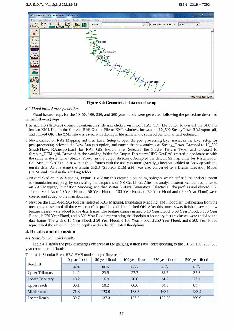
Table 4.1 shows the peak discharges observed at the gauging station (J80) corresponding to the 10, 50, 100, 250, 500

year return period floods.

Table 4.1: Sironko River HEC HMS model output flow results

Reach ID

10 year flood 50 year flood 100 year flood 250 year flood 500 year flood

m3/s m

3/s m

3/s m

3/s m

3/s

Upper Tributary 14.2 23.5 27.7 33.7 37.2

Lower Tributary 10.2 16.9 20.0 24.5 27.1

Upper reach 33.1 58.2 66.6 80.1 89.7

Middle reach 71.8 123.0 138.5 163.9 183.4

Lower Reach 80.7 137.3 157.6 188.00 209.9

G.J. E.D.T., Vol. 1(2) 2012:19-31 ISSN 2319 – 7293

28

Sironko HEC HMS model output flow data obtained were reasonable since the model was manually calibrated based on

observation of river flows at the gauging station. The output HEC HMS model flow data was therefore used as input data

for the Sironko RAS steady flow model.

Sironko HEC HMS model sensitivity analysis

To compare the sensitivity of HEC HMS Model River flows to the observed river flows, an index of the goodness-of-fit

value as known as objective function was computed. Several measures of objectives functions exist, however for this

research the most appropriate measure was the peak percentage error. Peak percentage error quantifies the fit as the

absolute value of the difference, expressed as a percentage, thus treating overestimates and underestimates as equally

undesirable (USACE, 2000). This objective function is a logical choice because the information provided in this research

is for planning purposes especially the case for a floodplain management to limit development in flood prone areas. The

objective functions (percentage peak errors) were estimated using equation (4.1). Model calibration was performed so as

to find reasonable parameters that would yield the minimum value of the objective function.

(4.1) 100%Q

QQerror Peak Percentage

o

om

Where Qm = model computed peak flows (m3/s)

Qo = Observed river peak flows (m3/s)

Sironko HEC HMS model calibration results

Sironko River HMS model was manually calibrated by varying the catchment basin Curve Number (CN) parameter

values. Reducing the CN parameter values by 10% resulted in under estimation of a 10 year flood by 2.48%, over

estimation of a 50 year flood by 2.45%, under estimation of a 100 year flood by 0.13%, under estimation of a 250 year

flood by 0.41%, and under estimation of a 500 year flood by 0.43% at the river gauging station (J80). The percentage

peak errors obtained were all less than 5%, this implies that the model developed was reliable.

4.2 Hydraulic model results

Sironko HEC RAS model output flow data (total discharges (Q Total)) was observed at the gauging station cross

section 7237.655 of the river middle reach. Other output data such as flood velocities in the channel (Vel Chnl), flow

area, top width of the channel, and the maximum flood depth in the channel (Max Chnl Depth) are as shown in Table 4.2.

Table 4.2: Sironko HEC RAS model output flow results at the gauging station

S/No Reach River

Station

Profile Q Total Vel Chnl Flow

Area

Top

Width

Max Chnl

Depth

(cfs) (ft/s) (sq ft) (ft) (ft)

1 Middle Reach 7237.655 10 Year Flood 2535.6 2.23 1152.02 100.95 17.1

2 Middle Reach 7237.655 50 Year Flood 4343.71 2.81 1609.97 109.98 21.43

3 Middle Reach 7237.655 100 Year Flood 4891.09 2.97 1722.38 111.9 22.45

4 Middle Reach 7237.655 250 Year Flood 5788.08 3.23 1897.34 114.83 23.99

5 Middle Reach 7237.655 500 Year Flood 6476.72 3.41 2025.12 116.92 25.09

Geometrical data model: River Sironko cross section bank stations and bridges were calibrated based on surveyed field data before use in the model. In calibrating cross sections, some river cross sections were removed while other cross

sections were introduced where they were insufficient in a given river reach in HEC RAS application.

Manning’s n values: Sironko river Upper reach down to the bridge 2, the channel had rocks, over banks had

vegetation and crops, from visual observation of the level of growth and nature of vegetation on over banks, the

appropriate range of manning’s values for the flood plain (Upper reach mountain streams) was taken as 0.04 – 0.045 for

field crops and high grass. For the main channel (with rocks), the appropriate manning’s values taken was 0.03 – 0.035.

Tributaries, Middle and lower reach, the over banks were bushy with no rocks in the main channel. Overbanks range of

manning’s n values selected was 0.050 – 0.055 and Main Channel range of manning’s n values selected was 0.035 –

0.23. Manning’s values were varied such that the maximum channel flood depth for a 10 year flood of 71.8 m3/s at the

gauging station was 5.21m. Past floods of magnitudes 63.45 m3/s, 65.93 m

3/s, and 67.77 m

3/s had channel flood depths of

4.91m, 4.79m, and 4.79m respectively at the river gauging station.

Sironko HEC RAS model calibration

The model was manually calibrated based on the maximum channel flood depths of past historical floods at the

gauging station located at bridge 1. It was observed that for higher steady flow input data values, the model channel flood

depths at the same gauging station were also higher. Sironko river geometrical data, bridges 1, 2, 3, and 4, and Manning’s

n values were calibrated based on field observations and field data obtained. Manning’s n values were further varied until

the desired maximum channel flood depth at the gauging station located at the bridge was obtained.

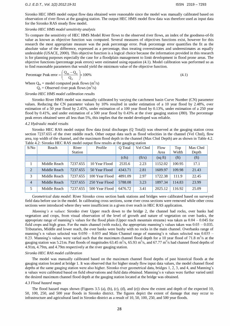
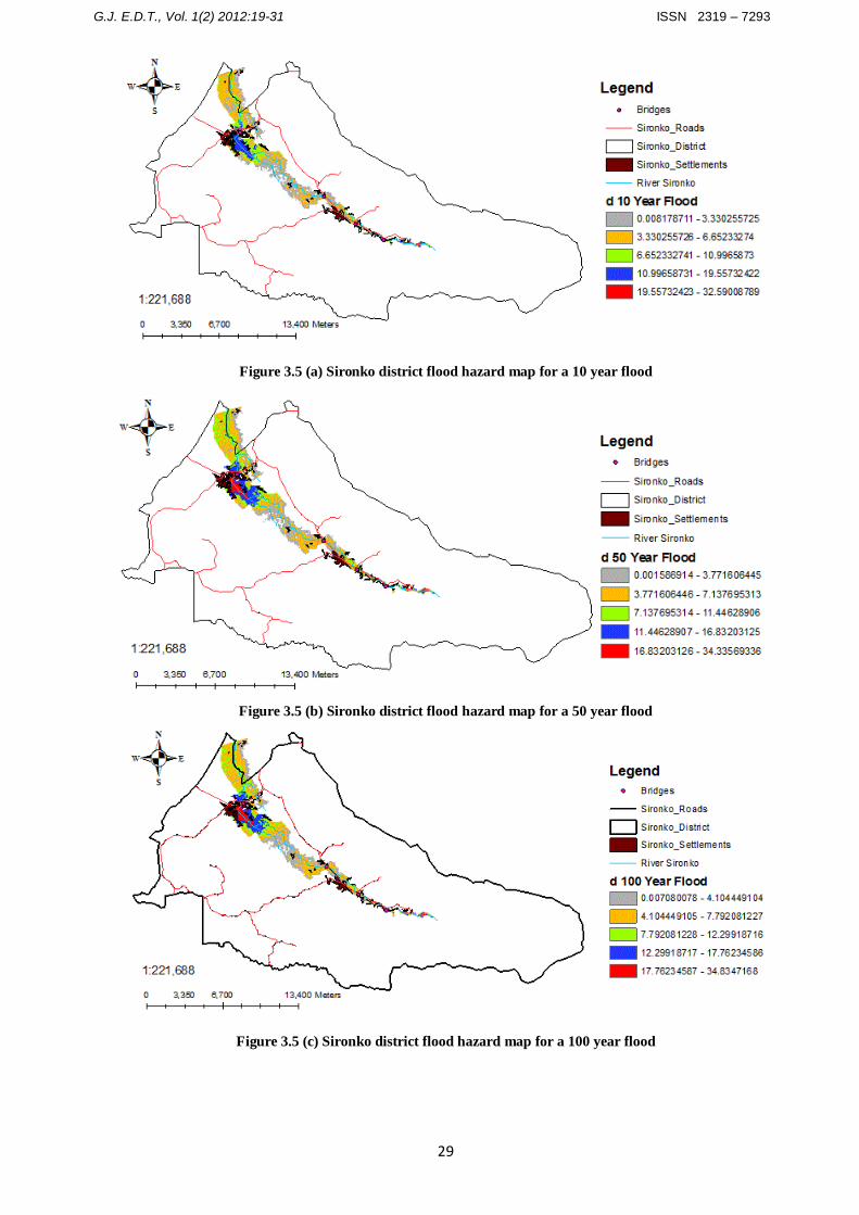
4.3 Flood hazard maps

The flood hazard maps shown (Figures 3.5 (a), (b), (c), (d), and (e)) show the extent and depth of the expected 10,

50, 100, 250, and 500 year floods in Sironko district. The figures depict the extent of damage that may occur to

infrastructure and agricultural land in Sironko district as a result of 10, 50, 100, 250, and 500 year floods.

G.J. E.D.T., Vol. 1(2) 2012:19-31 ISSN 2319 – 7293

29

Figure 3.5 (a) Sironko district flood hazard map for a 10 year flood

Figure 3.5 (b) Sironko district flood hazard map for a 50 year flood

Figure 3.5 (c) Sironko district flood hazard map for a 100 year flood

G.J. E.D.T., Vol. 1(2) 2012:19-31 ISSN 2319 – 7293

30

Figure 3.5 (d) Sironko district flood hazard map for a 250 year flood

Figure 3.5 (e) Flood hazard map for a 500 year flood

5. Conclusions and recommendations

5.1 Hydrological modeling

Hydrological modeling (rainfall – runoff analysis) was successfully performed using HEC HMS computer software

version 3.5. After developing the basin model component using HEC GeoHMS in ArcGIS environment, populating the

meteorological model and defining the control specifications, Sironko HMS was run while calibrating the parameters.

The model output results were the quantified runoff floods that resulted from input rainfall data. The 10, 50, 100, 250,

and 500 year design storms (rainfall) of 96.93mm, 130.90mm, 145.54mm, 164.88mm, and 179.51mm data input into

Sironko HMS model generated runoff (flood discharges) of 71.8 m3/s, 123.0 m

3/s, 138.5 m

3/s, 163.9 m

3/s, and 183.4 m

3/s

magnitudes respectively.

5.2 Hydraulic modeling

Sironko RAS hydraulic model was calibrated and then used to simulate the 10, 50, 100, 250, and 500 year floods of 71.8

m3/s, 123.0 m

3/s, 138.5 m

3/s, 163.9 m

3/s, and 183.4 m

3/s magnitudes respectively to determine maximum channel flood

depths for all river cross sections. The model maximum channel flood depths at the gauging station river cross section

located close to bridge 1 were 5.21m, 6.53m, 6.84m, 7.31m, and 7.65m for the simulated 10, 50, 100, 250, and 500 year

design floods respectively.

5.3 Flood hazard maps

The flood hazard maps for the 10, 50, 100, 250, and 500 year floods were generated as shown in Figures 3.5. From the

flood hazard maps developed, the most flood prone area is Sironko river middle reach. Also the some villages located in

the flood plain would be affected more especially with the 50, 100, 250, and 500 year floods.

5.4 Recommendations

G.J. E.D.T., Vol. 1(2) 2012:19-31 ISSN 2319 – 7293

31

The hydrological and hydraulic model were specifically developed for Sironko River in Sironko district, therefore they

cannot be adopted for any other location or river. However the methods used to model the floods can be repeated to

perform the same tasks in any location provided all the required datasets for that particular location are available. The

hydrological model, hydraulic model, and developed datasets are recommended for use only in Sironko district. The

software tools used in flood modeling do have help manuals that can be of great help in case the analyst experiences any

difficulties when analyzing/processing the data sets.

6. Challenges encountered

6.1 Datasets

There was only one rain-gauge station located within the catchment basin of river Sironko from which rainfall data was

obtained. This meant that there was a great variation of rainfall over the entire catchment basin. To solve this challenge,

the river flow data at the gauging station was used to calibrate the hydrological model so as to establish reliable river

flows in the five river reaches.

DEM downloaded from the US Geological Survey (USGS) website seemed to be of very poor resolution; therefore the

Uganda DEM obtained from the department of GIS and Survey of cell size 92.52m by 92.52m was used. By the time the

research was conducted, this was the DEM was the best resolution.

7. Acknowledgements

The authors extend their gratitude to Busitema University management for the financial support towards key activities of

the research project such as field surveys and acquisition of pertinent data such as rainfall data, river flow data, the

Digital Elevation Model (DEM), land use cover data layers, etc.

8. References

Abhas K Jha, Robin Bloch, and Jessica Lamond. (2012). Cities and Flooding; A Guide to Integrated Urban Flood Risk Management

for the 21st Century, electronic document. Retrieved from

http://www.gfdrr.org/gfdrr/sites/gfdrr.org/files/urbanfloods/pdf/Cities%20and%20Flooding%20Guidebook.pdf. Accessed 21 November 2012.

Central intelligence Agency (CIA) World Factbook. Population growth rate, electronic document. Retrieved from https://www.cia.gov/library/publications/the-world-factbook/fields/2002.html. Accessed 15 November 2012.

Dartmouth Flood Observatory (DFO). (2011). Green Flood Alert in Uganda, electronic document. Retrieved from

http://www.dartmouth.edu/~floods/Archives/2011sum.htm. Accessed 12 September, 2012

David Butler & John W. Davies. (2004). Urban Drainage.11 New Fetter Lane, London EC4P 4EE: Spon Press, Taylor & Francis e-

Library

Department for international development (DFID). Source book for sustainable flood mitigation strategies, electronic document.

Retrieved from http://www.dfid.gov.uk/r4d/PDF/Outputs/Water/R8159-Source_Book.pdf. Accessed 21 November 2012.

Environmental Systems Research Institute (ESRI). (2003). Arc Hydro Tools - Tutorial: Version 1.1 Beta 2. New York - United States

of America: Elmer Holmes Bobst library.

Environmental Systems Research Institute (ESRI). (2009). Introduction to ArcGIS 9.3. New York - United States of America: Elmer Holmes Bobst library.

Maidment, D. R. & Seth Ahrens. (1999). Introduction to HEC – HMS: CE 394k.2 Surface Water hydrology, electronic document. Retrieved from http://www.ce.utexas.edu/prof/maidment/grad/tate/research/RASExercise/webfiles/hecras.html. Accessed 17

September 2012

Sironko District, electronic document. Retrieved from http://en.wikipedia.org/wiki/Sironko_District. Accessed 10th October 2012

Uganda National Water Development (UNWD) – Report (2005), electronic document. Retrieved from

http://unesdoc.unesco.org/images/0014/001467/146760e.pdf. Accessed 14 November 2012

US Army Corps of Engineers (USACE). (2000). Hydrologic Modeling System HEC-HMS: Technical reference manual. Hydrologic

Engineering Center, Davis, CA – United States of America.

US Army Corps of Engineers (USACE). (2008). Hydrologic Modeling System HEC-HMS: Applications Guide. Hydrologic

Engineering Center, Davis, CA – United States of America.

US Army Corps of Engineers (USACE). (2010). River Analysis System HEC-RAS: Applications Guide. Hydrologic Engineering

Center, Davis, CA – United States of America.