Embed Size (px)
Citation preview

Application of Holomorphic Embedding to the Power-Flow Problem
by
Muthu Kumar Subramanian
A Thesis Presented in Partial Fulfillment
of the Requirements for the Degree
Master of Science
Approved July 2014 by the
Graduate Supervisory Committee:
Daniel Tylavsky, Chair
John Undrill
Gerald Heydt
ARIZONA STATE UNIVERSITY
August 2014

i
ABSTRACT
With the power system being increasingly operated near its limits, there is an
increasing need for a power-flow (PF) solution devoid of convergence issues.
Traditional iterative methods are extremely initial-estimate dependent and not
guaranteed to converge to the required solution. Holomorphic Embedding (HE) is a
novel non-iterative procedure for solving the PF problem. While the theory behind a
restricted version of the method is well rooted in complex analysis, holomorphic
functions and algebraic curves, the practical implementation of the method requires
going beyond the published details and involves numerical issues related to Taylor’s
series expansion, Padé approximants, convolution and solving linear matrix equations.
The HE power flow was developed by a non-electrical engineer with language
that is foreign to most engineers. One purpose of this document to describe the
approach using electric-power engineering parlance and provide an understanding
rooted in electric power concepts. This understanding of the methodology is gained
by applying the approach to a two-bus dc PF problem and then gradually from
moving from this simple two-bus dc PF problem to the general ac PF case.
Software to implement the HE method was developed using MATLAB and
numerical tests were carried out on small and medium sized systems to validate the
approach. Implementation of different analytic continuation techniques is included
and their relevance in applications such as evaluating the voltage solution and

ii
estimating the bifurcation point (BP) is discussed. The ability of the HE method to
trace the PV curve of the system is identified.

iii
ACKNOWLEDGEMENTS
First, I would like to express my sincere thanks to Dr. Tylavsky, my advisor for
being a commendable source of knowledge and inspiration. From the beginning of my
graduate career, he has inculcated a passion for the subject, guided me through several
challenges in research and shaped my writing skills.
I express my sincere thanks to Yang Feng, doctoral student at ASU. Yang brought
me up to speed on the work being done in the research group. The endless hours of
discussion with him has molded my research. I consider it my privilege to have worked
alongside such a wonderful person.
Dr. Antonio Trias, Gridquant Inc., deserves a special mention for the valuable
inputs he gave to our research group. I would like to extend to my thanks to my
graduate committee members Dr. Heydt and Dr. Undrill for their valuable feedback and
suggestions to my thesis document. I am grateful to the all the faculty members of
power engineering for the wonderful learning experience they provided for the last two
years.
I would like to express my gratitude to the School of Electrical, Computer and
Energy Engineering for providing me the opportunity to work as Teaching Assistant.
Finally, my heart is with my family and friends who have kept me grounded during the
entire period of my study.

iv
TABLE OF CONTENTS
Page
LIST OF FIGURES ...................................................................................................... ix
LIST OF TABLES ......................................................................................................... x
NOMENCLATURE ..................................................................................................... xi
CHAPTER
1 INTRODUCTION ................................................................................................... 1
1.1 Power-flow Problem ................................................................................ 1
1.2 Voltage Stability Problem ........................................................................ 2
1.3 Holomorphically Embedded Power-Flow Formulation........................... 3
1.4 Objective .................................................................................................. 4
1.5 Organization ............................................................................................. 4
2 LITERATURE REVIEW ........................................................................................ 6
2.1 Solution Methodologies to the Power-Flow Problem .............................. 6
2.1.1 Gauss-Seidel Method ............................................................... 8
2.1.2 Newton-Raphson Method ........................................................ 9
2.1.3 Algorithmic Improvements To Newton’s Method ................ 11
2.1.4 Fast Decoupled Load Flow Method ...................................... 11
2.1.5 Series Load Flow ................................................................... 13
2.2 Need for a Non-iterative Approach ........................................................ 14

v
CHAPTER Page
2.3 Evaluating the Saddle Node Bifurcation Point ...................................... 18
2.3.1 Continuation Method ............................................................. 19
2.3.2 Direct Method for Evaluating Bifurcation Point ................... 20
2.3.3 Optimization Techniques ....................................................... 21
3 ANALYTIC CONTINUATION ............................................................................ 22
3.1 Introduction ............................................................................................ 22
3.2 Direct Method (Matrix Method) ............................................................ 25
3.3 Viskovatov Method ................................................................................ 28
3.4 Epsilon Algorithm .................................................................................. 31
3.5 Numerical Illustration of Analytic Continuation ................................... 33
3.5.1 Padé Approximants using Matrix Method............................. 34
3.5.2Continued Fraction ................................................................. 35
3.5.3 Epsilon Algorithm ................................................................. 36
3.5.3 Acceleration Of Convergence Of π Series ............................ 36
3.6 Numerical Issues in Evaluating the Analytic Continuation ................... 41
3.6.1 Degenerate Power Series ....................................................... 42
3.6.2 Ill-Conditioned Padé Matrix in Evaluating a Convergent
Series .................................................................................. 45

vi
CHAPTER Page
4 SOLVING A GENERAL CASE POWER-FLOW PROBLEM WITH
HOLOMORPHIC EMBEDDING ......................................................................... 50
4.1 Introduction to Holomorphic Embedding .............................................. 50
4.1.1 Holomorphic Functions ......................................................... 50
4.1.2 Load Bus Modeling Using HE .............................................. 51
4.1.3 Germ Solution for Load Bus Model ...................................... 52
4.1.4 Power Series Expansion ........................................................ 54
4.2 Generator Bus Model I using Holomorphic Embedding ........................... 57
4.2.1 Germ Solution for the Generator Bus Model I .................. 62
4.2.2 Evaluating Power Series Coefficients for Generator Bus
Model I ............................................................................... 64
4.3 Generator Bus Model II Using HE ........................................................ 70
4.3.1 Evaluating Voltage Series Coefficients for Generator Bus
Model II ............................................................................. 73
4.4 Power-Flow Solution using HE ............................................................. 79
4.4.1 Handling Reactive Power Limits of Generator ..................... 79
4.4.2 Convergence Criteria ............................................................. 81
4.4.3 Flowchart ............................................................................... 81
vii
CHAPTER Page
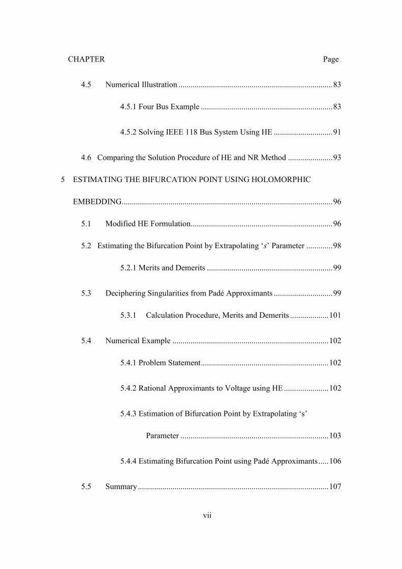
4.5 Numerical Illustration ............................................................................ 83
4.5.1 Four Bus Example ................................................................. 83
4.5.2 Solving IEEE 118 Bus System Using HE ............................. 91
4.6 Comparing the Solution Procedure of HE and NR Method ...................... 93
5 ESTIMATING THE BIFURCATION POINT USING HOLOMORPHIC
EMBEDDING ........................................................................................................ 96
5.1 Modified HE Formulation...................................................................... 96
5.2 Estimating the Bifurcation Point by Extrapolating ‘s’ Parameter ............. 98
5.2.1 Merits and Demerits .............................................................. 99
5.3 Deciphering Singularities from Padé Approximants ............................. 99
5.3.1 Calculation Procedure, Merits and Demerits ................... 101
5.4 Numerical Example ............................................................................. 102
5.4.1 Problem Statement ............................................................... 102
5.4.2 Rational Approximants to Voltage using HE ...................... 102
5.4.3 Estimation of Bifurcation Point by Extrapolating ‘s’
Parameter ......................................................................... 103
5.4.4 Estimating Bifurcation Point using Padé Approximants ..... 106
5.5 Summary .............................................................................................. 107

viii
CHAPTER Page
6 CONCLUSION AND FUTURE WORK ............................................................ 109
6.1 Conclusion ........................................................................................... 109
6.2 Future Work ......................................................................................... 110
6.2 REFERENCES .................................................................................................... 112
APPENDIX A VOLTAGE SOLUTION FOR IEEE 118 BUS SYSTEM ................ 117

ix
LIST OF FIGURES
Figure Page
2.1 Convergence Problems in Iterative Methods: Two-bus Example ................. 15
2.2 Initial Estimate Dependency of NR Method .................................................. 16
2.3 Initial Estimate Dependency of the FDLF Method........................................ 18
3.1 Radius of Convergence of Power Series f1(s) ................................................ 23
3.2 Domain of Convergence of f1(s), f2(s) and f3(s) ............................................. 24
3.3 Convergence of Power Series vs. Padé Approximant ................................... 40
3.4 Solving a dc PF problem using the HE procedure ......................................... 45
4.1 Sample Three-bus Test System ...................................................................... 68
4.2 Solution Procedure using Holomorphic Embedding ..................................... 82
4.3 One Line Diagram of Sample Four- bus System ........................................... 83
4.4 Recurrence Relation to Calculate Power Series Coefficients for Four-bus
Problem (Generator Bus Model I) ............................................................... 86
4.5 Recurrence Relation to Calculate Power Series Coefficients for Four-bus
Problem (Generator Bus Model II) .............................................................. 88
4.6 Convergence Properties of HE procedure...................................................... 91
5.1 Accuracy of Bifurcation Point obtained by Extrapolating s ........................ 104
5.2 Bus Voltages vs. Loading Parameter for Four-bus System ......................... 105
5.3 Estimate of Bifurcation Point Obtained from Padé Approximant ............... 107
5.4 Error in Bifurcation Point Obtained from Padé Approximant ..................... 107
x
LIST OF TABLES
Table Page
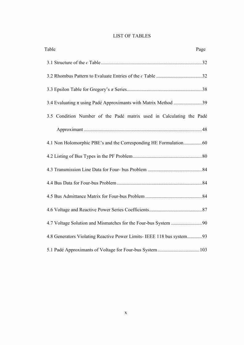
3.1 Structure of the ϵ Table .................................................................................. 32
3.2 Rhombus Pattern to Evaluate Entries of the ϵ Table ..................................... 32
3.3 Epsilon Table for Gregory’s π Series ............................................................. 38
3.4 Evaluating π using Padé Approximants with Matrix Method ....................... 39
3.5 Condition Number of the Padé matrix used in Calculating the Padé
Approximant ................................................................................................ 48
4.1 Non Holomorphic PBE’s and the Corresponding HE Formulation............... 60
4.2 Listing of Bus Types in the PF Problem ........................................................ 80
4.3 Transmission Line Data for Four- bus Problem ............................................ 84
4.4 Bus Data for Four-bus Problem ..................................................................... 84
4.5 Bus Admittance Matrix for Four-bus Problem .............................................. 84
4.6 Voltage and Reactive Power Series Coefficients........................................... 87
4.7 Voltage Solution and Mismatches for the Four-bus System ......................... 90
4.8 Generators Violating Reactive Power Limits- IEEE 118 bus system ............ 93
5.1 Padé Approximants of Voltage for Four-bus System .................................. 103

xi
NOMENCLATURE
|Vi | Voltage magnitude at bus i
a, b Scalars
An(s) The nth
order numerator term in three term recursive relation
B', B'' Approximations to Jacobian matrix in FDLF method
Bik Line susceptance between bus i and bus k
Bn(s) The nth
order denominator term in three term recursive relation
BP Bifurcation point
BPEE Bus Power Equilibrium Equation
C Set of complex numbers
c(i)
[n] n-th order term in the continued fraction
c1(s) Partial power series in the Viskovatov method
CPF Continuation Power-flow
f [n] Power series coefficient of degree n for function f
f(s) Power series representation of function f using parameter s
FDLF Fast Decoupled Power-flow
fn Another notation for power series coefficient of degree n
Gik Line conductance between bus i and bus k
GS Gauss-Seidel
HE Holomorphic Embedding

xii
HV High voltage
Jik Jacobian matrix entry in NR method
L Degree of numerator polynomial in the Padé approximant
LHS Left hand side
LV Low voltage
M Degree of denominator polynomial in the Padé approximant
m Set of PQ buses
N Number of buses in a power system
n Used to indicate the degree of s in the power series
NR Newton-Raphson
p Set of PV buses
PBE Power balance equation
PF Power-flow
PGi Real power generated at bus i
Pi Real power injection at bus i
PLi Real power load at bus i
PV bus Generator bus/ Voltage bus
PV curve Power voltage curve
Q(s)
Reactive power represented as a power series in generator bus
model I

xiii
QGi Reactive power generated at bus i
QGi MAX Maximum reactive power limit of generator at bus i
QGi MIN Minimum reactive power limit of generator at bus i
Qi Reactive power injection at bus i
QLi Reactive power load at bus i
R Transmission line resistance
RHS Right hand side
Rhs_Known
Intermediate value in the calculation of the RHS vector in
generator bus model I
s Complex variable used in holomorphic embedding
Si Complex power injection at bus i
slack Slack bus
Vi Per unit voltage at bus i
Vi im[n] Imaginary part of the voltage series coefficient of degree n
Vi re[n] Real part of the voltage series coefficient of degree n
Vi sp
Specified voltage at bus i
Vi(0) Voltage function for bus i evaluated at s=0/ germ solution
Vi(1) Voltage series for bus i evaluated at s=1.
Vi(s) Voltage power series for bus i
Vi[n] n-th order voltage series coefficients of bus i

xiv
VS Voltage stability
Vslack Slack bus voltage
Wi(s) Inverse voltage series for bus i
Wi[n] n-th order inverse voltage series coefficients of bus i
X Transmission line reactance
Y Bus admittance matrix
Yi shunt Shunt component of the bus admittance matrix at bus i
Yik Admittance bus matrix entry between bus i and bus k
Yik trans
Series component of the bus admittance matrix between buses i
and k
Z Transmission line impedance
βik
Coefficient of iteration matrix corresponding to Vk re[n] for
generator bus i in generator bus model II
γik
Coefficient of iteration matrix corresponding to Vk im[n] for
generator bus i in generator bus model II
ϵk j
Entry of kth
column in the epsilon table. j measures the
progression down the column
ζi[n-1]
RHS element obtained from real power constraint in PV bus
model II
θi Voltage angle at bus i

xv
κ(A) Condition number of matrix A
λ Loading parameter

1
1 INTRODUCTION
1.1 POWER-FLOW PROBLEM
Power-flow (PF) studies are of primal importance in reliable operation of existing
power system. Solving the PF problem constitutes an integral part of reliability studies
such as contingency analysis, planning processes such as generation expansion
planning and transmission expansion planning; also, the PF solution provides the initial
point for dynamic simulation of power system components. The objective of the
traditional PF problem is to find the static operating point of a balanced three-phase
power system [1]. Given the network topology and its parameters, the complex power
injections at load buses, the real power injection and voltage magnitude at generator
buses, the primary results obtained from PF studies are bus voltage magnitudes and
angles for load/PQ buses and bus voltage angles and reactive power for generator/PV
buses. Secondary results such as flows across transmission lines, transformers,
generator reactive power output, losses in the network can be calculated from the
voltage solution.
Iterative methods such as Gauss-Seidel (GS), Newton-Raphson (NR), Fast
Decoupled Load Flow (FDLF) and their many variants [2]-[6] are being used
ubiquitously in the industry for solving the PF problem. While they appear to work well
under normal loading conditions, as the loading increases, they can and do fail to
converge [7], [8]. Furthermore, the trajectory that is taken by the iterative methods to
approach the voltage solution is initial estimate dependent. For the power-flow problem,

2
which has multiple solutions, this means that these methods do not have a guarantee of
convergence to the desired solution. All these problems have been addressed from time
to time in the literature by proposing algorithmic enhancements to the existing methods
[9]-[14]. However, a globally acceptable procedure to solve the convergence issues of
iterative methods has yet to be developed.
1.2 VOLTAGE STABILITY PROBLEM
Voltage stability (VS) is defined as the ability of the power system to maintain
steady-state voltages at all the buses after being subjected to a disturbance from a given
initial operating condition [15]. The phenomenon of voltage instability (or voltage
collapse) is responsible for major blackouts in the history of electric power industry;
some of the major incidents reported worldwide are catalogued in [16], [17]. For a
simple two-bus problem that has two solutions (high-voltage and low-voltage solutions)
voltage collapse is said to occur when both the solutions coalesce. This idea can be
easily extended to a general N-bus problem. Even an infinitesimal increase in loading
beyond the voltage collapse point, also known as the bifurcation point (BP), results in
no voltage solution to the PF problem. Traditional Newton-Raphson type methods fail
to converge near the maximum loading point since the Jacobian matrix becomes
ill-conditioned (approaches singularity), causing numerical errors in calculating the
voltage solution. In the present voltage stability analysis practices, the PV curve
obtained from some form of continuation power-flow (CPF) [18], [19] is a byproduct of
3
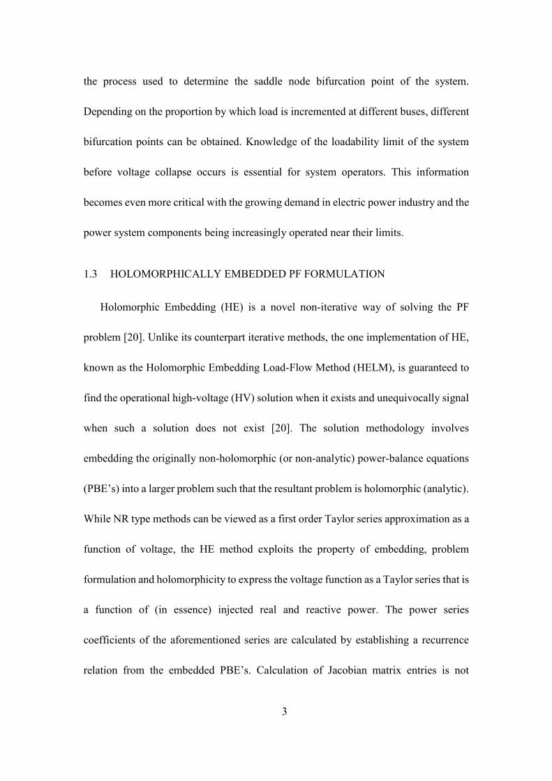
the process used to determine the saddle node bifurcation point of the system.
Depending on the proportion by which load is incremented at different buses, different
bifurcation points can be obtained. Knowledge of the loadability limit of the system
before voltage collapse occurs is essential for system operators. This information
becomes even more critical with the growing demand in electric power industry and the
power system components being increasingly operated near their limits.
1.3 HOLOMORPHICALLY EMBEDDED PF FORMULATION
Holomorphic Embedding (HE) is a novel non-iterative way of solving the PF
problem [20]. Unlike its counterpart iterative methods, the one implementation of HE,
known as the Holomorphic Embedding Load-Flow Method (HELM), is guaranteed to
find the operational high-voltage (HV) solution when it exists and unequivocally signal
when such a solution does not exist [20]. The solution methodology involves
embedding the originally non-holomorphic (or non-analytic) power-balance equations
(PBE’s) into a larger problem such that the resultant problem is holomorphic (analytic).
While NR type methods can be viewed as a first order Taylor series approximation as a
function of voltage, the HE method exploits the property of embedding, problem
formulation and holomorphicity to express the voltage function as a Taylor series that is
a function of (in essence) injected real and reactive power. The power series
coefficients of the aforementioned series are calculated by establishing a recurrence
relation from the embedded PBE’s. Calculation of Jacobian matrix entries is not

4
involved in this solution procedure. Solving the PF problem using HE for a system of
PQ buses (and one slack bus) is discussed in [21].
1.4 OBJECTIVE
The objective of this work is to apply the novel HE method to solve the general ac
PF problem. This report covers the following topic areas.
1. Introduce the concept of analytic continuation and elucidate its relevance to
the HE procedure.
2. Explore several techniques of analytic continuation and their numerical
implementation.
3. Introduce the existing load-bus model and analyze the development of the
two different generator bus models in detail.
4. Develop a solution procedure for solving the general case PF problem.
5. Compare the solution procedure of the HE method with NR method.
6. Develop a HE that can be used in estimating the saddle-node bifurcation
point of the system with PQ buses.
1.5 ORGANIZATION
The report is organized into five additional chapters. The content of each chapter is
discussed in brief below.
Chapter 2 is a review of the existing literature of PF methods and present practices
in evaluating the BP of the system.
The concept of analytic continuation and its relevance to the solution methodology
is presented in Chapter 3. Three different techniques of calculating analytic

5
continuation are explored with numerical examples, their merits and demerits in the
context of solving the PF problem are explained.
In Chapter 4, the existing literature about the load bus model is introduced. The
development of two different generator bus models using HE method and its
incorporation in solving the general PF problem is discussed in detail. Test results from
the IEEE 118 bus system are presented; the solution is validated against the results from
commercial PF software.
Estimating the BP of a system with PQ buses using the HE procedure is discussed
in Chapter 5. The estimate is compared against the actual value of BP obtained from
existing CPF method.
Chapter 6 presents a summary of the reported work and scope for the future work.

6
2 LITERATURE REVIEW
The literature review will focus on the following: First, the developments in solving
the PF problem are described. Next, the initial-estimate-dependency of iterative
methods is illustrated. Finally, the literature on evaluating the BP of the system is
discussed.
2.1 SOLUTION METHODOLOGIES TO THE POWER-FLOW PROBLEM
The power-flow problem involves solving the nonlinear system of PBE’s. The
numerical techniques employed to solve the PF problem have evolved over the years.
Nevertheless, the quest for a single “best” method that caters to problems of all sizes
and types with minimal computing requirements and desired convergence properties is
still a work in progress.
The real and reactive power injections at every bus i, for an N-bus system can be
related to the bus voltages, the system topology and the network parameters as follows:
)sin()cos(
0
kiikkiik
N
k
kii BGVVP
)cos()sin(
0
kiikkiik
N
k
kii BGVVQ
(2.1)
Equation (2.1) is referred to as the hybrid formulation where the bus admittance
matrix (Y bus) entries are written in rectangular form and bus voltages are expressed in
polar form. Equation (2.1) also constitutes the defining equations for a load bus, i, for a
N-bus system whose complex power injections are known and complex voltages are
unknown.

7
For a generator bus, the real power injection into the bus is known. The bus voltage
magnitude is maintained to be constant by varying the quantity of VARS injected into
the network. The defining equations for a generator bus, i, are:
)sin()cos(0
kiikkiik
N
k
kii BGVVP
spii VV
(2.2)
A slack bus is necessary to compensate for the losses in the system. The voltage
magnitude and angle are fixed for the slack bus. The real and reactive power injections
are taken as free variables. Hence, for a slack bus,
spii VV
spii
(2.3)
Mathematically, for an N-bus system with one slack bus, there are up to 2N-1
voltage
solutions. Of the possible solutions, only one solution corresponds to the operable
solution also referred to as the HV solution. Iterative methods such as NR and FDLF
with a “reasonable” estimate generally converge to the required HV solution. However,
several factors such as poor initial estimate, high R/X ratio (typical of distribution
systems) and operation near the maximum loading point can lead to ill-conditioned
matrices [7] resulting in convergence issues.

8
2.1.1 GAUSS-SEIDEL METHOD
In the history of solving the ac PF problem, GS method was the first method to be
implemented in digital computers. The nonlinear PBE for a load bus in (2.1) can be
alternatively expressed as a “weakly linear” [22] system of equations as:
*
*
1 i
i
N
k
kikiV
SVYI
(2.4)
Equation (2.4) is still nonlinear because the bus voltages in the denominator and
hence current injection into the bus are unknown. From (2.4), an iteration scheme is
established to calculate the bus voltages [1].
N
ik
kik
i
k
kik
i
ii
ii
i nVYnVYnV
jQP
YnV
1
1
1
*)()1(
)(
1)1( (2.5)
The coefficient n in equation (2.5) is the iteration index. The Gauss-Seidel method
is a fixed point form with the bus voltages as variables. Starting with an initial estimate
of bus voltages, using the complex power specified at each bus and the network
parameters, a new vector of bus-voltage estimates Vi(n+1) is obtained. The estimate of
bus voltage for bus i, at iteration n+1, (Vi(n+1)) is expressed as a function of the most
recently updated value of voltages up to bus i-1. For generator buses, the reactive power
injection is unknown; it can be calculated from the updated value of bus voltages. The
iteration process described in (2.5) is repeated until the difference between two
successive voltage estimates is less than a pre-determined tolerance value. The GS
method is easier to program; there is no need of factorizing a sparse matrix. The

9
memory requirements for the GS method are minimal; for an N-bus system, it is
directly proportional to the system size N [23]. The Gauss-Seidel method has linear
convergence characteristics [1].
In equation (2.5), only the buses connected to bus i are required to calculate the
updated value of Vi(n+1). The calculation of such bus voltages can be carried out
independent of the remaining network. A larger problem can thus be split into a
sequence of smaller problems based on the bus adjacency matrix and processed in
parallel. Reference [24] presents a theoretical upper bound of speed up for different
implementations of parallelized GS method. The computation time for the traditional
GS method increases proportional to N2[22].
2.1.2 NEWTON-RAPHSON METHOD
The NR method for solving nonlinear power-balance equations (PBE’s) is a
recursive method that solves a linear system of equations at each iteration; the linear
equations are derived from a first order Taylor’s series approximation of the function at
the best estimate of the solution point. Since the PBE’s are non-analytic, they cannot be
differentiated in the complex form. Hence, the variables are broken down into real
variables in either polar form or rectangular form. The first order partial derivatives of
the PBE with respect to the bus voltage magnitude and angle (assuming polar form of
the variables is used) constitute the entries of the Jacobian matrix. The Jacobian matrix
evaluated at a particular point is representative of the slope of tangent vector to the PBE

10
at that point. Using this process, a linear system of equations that relates the Jacobian
matrix and mismatches in the PBE’s is obtained. A simplified version of the above
mentioned linear relation is:
VJJ
JJ
Q
P
2221
1211 (2.6)
where J11, J12, J21 and J22 are the entries of the Jacobian matrix defined in [1]. The
entries ΔP, ΔQ are the mismatch in the PBE’s and Δθ, ΔV denote the update in bus
voltage angle and magnitude respectively. In solving a N-bus system using the NR
method, the equation corresponding to the slack bus in (2.6) can be eliminated. For a
PV bus, the ΔQ equation is absent in (2.6). After, correcting for the slack buses and PV
buses, the solution to the linear system of equations (2.6) for all buses, yields an update
vector for system states (Δθ, ΔV); the updates are added to the current estimate of
voltage angle and magnitude (θ, V). The process is repeated iteratively until the
maximum mismatch in the PBE’s is less than a pre-determined value of tolerance. The
NR method has quadratic convergence properties. Stott [22] claims that the full NR
method converges in 2-5 iterations from a flat start initial estimate to the required
solution irrespective of the problem size. A practical PF with discrete elements in the
network such as on-load tap changing transformers (OLTC), phase shifters and FACTS
devices is much more complicated and requires a few more iterations to converge.

11
2.1.3 ALGORITHMIC IMPROVEMENTS TO NEWTON’S METHOD
Since the advent of NR method in solving the PF problem, several enhancements
have been proposed to improve its performance. A very trivial modification used to
obtain faster convergence is to use a previously calculated voltage solution as the initial
estimate instead of a flat start. Dishonest Newton methods use the same Jacobian
matrix for the successive iterations [3], thereby saving the costs of computing the
Jacobian and triangular matrix factorization for every iteration. Limits are sometimes
imposed on the maximum permissible change in the estimates to deal with the
non-smoothness in the function [25]. For a practical power system problem, the
Jacobian matrix is extremely sparse with very few non-zero elements in every row.
Hence, sparse matrix storage techniques and optimal ordering schemes to minimize the
number of fill-ins that occur during the triangular matrix factorization are employed to
reduce the computation time and storage requirements in NR method.
2.1.4 FAST DECOUPLED LOAD FLOW (FDLF) METHOD
Based on the typical characteristics of PF problems and through the experience
gained via numerical experimentation, a series of approximations were made to the
traditional NR method to produce what has become an industry standard known as the
Fast Decoupled Load Flow. For PF problems, under nominal operating conditions,
there is weak coupling between active power and voltage magnitudes; similarly, there
is weak coupling between reactive power and voltage angle. Hence, in the FDLF

12
formulation the corresponding entries in the Jacobian matrix are neglected, leading to
two decoupled system of equations that are solved independently [6]. Other
assumptions used in deriving the FDLF Jacobian matrix are very small R/X ratio
branches (typical of transmission systems) and small differences in voltage angle
between adjacent buses. The Jacobian is thus reduced to constant matrix independent of
the estimate of the system states, thereby saving the costs of updating and re-factorizing
the matrix. The speed per iteration is approximately five times that of the full NR
method [5]. The system of equations to be solved is reduced from (2.6) to:
VBVQ
BVP
''
' (2.7)
where B', B'' denote the constant approximations to the Jacobian matrix defined in [5].
One variation of the FDLF method is the X/B method. The elements of the B', B''
matrices are calculated in the X/B method [27] as:
N
ikk
ikii
ikik
ik
ik
N
ikk
ikii
ik
ik
BBXR
XB
BBX
B
1
''''
22
''
1
''' ,1
(2.8)
The number of iterations required to converge using the FDLF increased over that
needed with the NR method, but the computation time required per iteration drastically
decreased [5]. Overall, the time taken to solve the PF problem decreased; as a result, the
use of FDLF method has become more prevalent in the industry.
13
Reference [26] compares FDLF method with NR and GS methods based on
memory requirements, CPU time, convergence properties, number of iterations and
effects of low precision arithmetic on reliability of solution for medium and large sized
systems. The FDLF method was found to be the fastest among the three methods on all
the tested scenarios [26]. The convergence rate of FDLF method (assuming it
converges) is between the NR (quadratic convergence) and GS (linear convergence)
methods. One disadvantage of the FDLF method is it inherits the initial estimate
dependency and convergence problems, especially near the BP, from its NR roots.
2.1.5 SERIES LOAD FLOW
A non-iterative approach to solve the PF problem has been proposed in [28] and
tested on an eleven-bus system. Using a series reversion technique, the voltage variable
is represented as an explicit series. The work is further extended in [30] by using a
Taylor’s series expansion in the neighbourhood of a feasible operating point.
Sensitivity of voltages to the bus power injections could be directly determined using
this technique. However, the existing series power-flow methods use an analytical
representation of the iteration process rather than the original PBE’s and it is
impractical to obtain for large systems. In addition, they are initial estimate dependent
in the sense that the initial operating point has to be obtained using an iterative
approach.

14
2.2 NEED FOR A NON-ITERATIVE APPROACH
The PBE’s constitute a nonlinear coupled system of equations with multiple
solutions. When solving a nonlinear problem using an iterative approach, the
convergence issues that arise are manifold. First off, there is no guarantee that the
non-iterative approach will converge to a solution. If a PF case does not converge, there
is no way to know if a solution does not exist or if the iterative method is to blame for
the non-convergence. Also, there is little control over the solution to which the iterative
method converges.
For a simple two-bus ac PF problem, there exist two solutions for a specified value
of power injection: the HV solution and the LV solution. Typically, the HV solution is
desired for practical purposes such as grid operation. However, the LV solution also
finds some applications viz., in determining the unstable equilibrium points [39].
Depending on the initial estimate, NR method may converge to the HV solution or the
LV solution or may not converge at all. These problems are inherent in all iterative
methods applied to nonlinear problems and occur irrespective of the problem size. The
initial estimate dependency of iterative methods can be illustrated with a simple
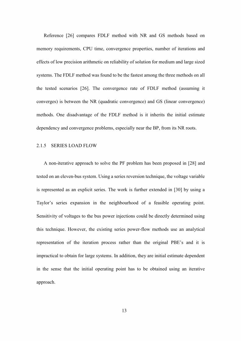
two-bus example shown in Figure 2.1. The system has one slack bus and one load bus
connected by a purely inductive transmission line. The system parameters are shown in
per unit quantities in Figure 2.1.
15
R=0
X=j0.2 p.u.
P2=1 p.u.
Q2=1 p.u.
V1 =1Ð 0 o|V2 |Ðθ2
Figure 2.1 Convergence Problems in Iterative Methods: Two-bus Example
The voltage solutions for the two-bus system calculated in closed form are:
a) HV solution = 0.6-j0.2=0.6324Ð-18.43 o
b) LV solution = 0.4-j0.2=0.4472Ð-22.56 o.
In order to demonstrate the initial estimate dependency of NR method, a
numerical experiment is conducted by solving the two-bus PF problem using NR
method with different initial estimates and categorizing the initial estimate based on
the solution to which the iterative method converges. The PBE’s for bus 2 for this
particular problem is derived from (2.1) are:
2
222
2
2221
2
22
221
2
5cos5cos
sin5sin
VVX
VVVQ
VX
VVP
(2.9)
The Jacobian matrix is obtained by taking the partial derivatives of the PBE
expressed in (2.9) with respect to the bus voltage magnitude and angle.
2
2
1
2222
222
2
2
10cos5sin5
sin5cos5
Q
P
VV
V
V
(2.10)
Starting from an initial estimate for the voltage magnitude and angle, the Jacobian
matrix and the mismatch in the PBE are evaluated from (2.9) and (2.10). By solving

16
the linear system of equations as described in (2.10), an update for bus voltage
magnitude and angle is found; Bus voltage magnitude and angle are updated and the
process is repeated until the mismatch in the PBE is less than 1e-04 p.u. The entire
procedure of solving the PF problem is repeated with different initial estimates for the
voltage. The initial estimate of the voltage magnitude is varied between 0.0 to 1.0 p.u.
in steps of 0.005 p.u. and the estimate of voltage angle is varied between –π to + π
radians in steps of 0.01 radians.
Depending on the starting point, the NR method can converge to either the HV
solution or the LV solution or does not converge at all. For this simple problem, the
NR method is assumed not to converge at all if it fails to reach either the HV solution
or the LV solution within 15 iterations. Figure 2.2 shows the plot of initial estimates
classified based on the solution to which they converge.
Figure 2.2 Initial Estimate Dependency of NR Method

17
In Figure 2.2, a red pixel indicates that, with that particular initial estimate of
voltage, the NR method converges to the LV solution. Similarly, a green pixel and
black pixel indicates convergence to HV solution and divergence respectively. The
plot reveals that even for the simplest of problems, the NR method used here does not
converge to the solution reliably.
Fast Decouple Power Flow (FDLF) method, being a variant of the NR method, also
suffers from the problem of initial-estimate dependency. To demonstrate the same, the
two-bus example shown in Figure 2.1 is solved using the X/B variation of the FDLF
method. The B', B'' matrices constructed from (2.8) are:
52.0
2.0
52.0
11
22
12
2
12
12''
22
12
'
22
XR
XB
XB
(2.11)
The iteration scheme for the two-bus problem (2.7) becomes:
2222
2
2222
2
2.0''
2.0'
VQB
VQV
VPB
VP
(2.12)
The decoupled system of equations is solved by adopting a (1θ-1V) iteration. The
two-bus problem is solved using FDLF with different initial estimates of the voltage (0
to 1 p.u. for voltage magnitude, –π to + π radians for voltage angle) at bus 2. The
criterion for convergence is a mismatch of less than 1e-04 in the PBE’s. The initial
estimates are categorized based on the solution to which FDLF method converges and
plotted in Figure 2.3.

18
Figure 2.3 Initial Estimate Dependency of the FDLF Method
The convergence issues that can arise from iterative methods are evident from the
above illustration. Also the when the system moves into extremis and the voltages
move far from nominal, the iterative methods can and do fail to converge due to an
ill-conditioned Jacobian matrix [29].
2.3 EVALUATING THE SADDLE NODE BIFURCATION POINT
In power system analysis, the BP (also known as the voltage collapse point), is
representative of the maximum power transfer to a bus in the system. Methods for
finding BP’s can be broadly classified into three categories: continuation method,
direct method and optimization method.
19
2.3.1 CONTINUATION METHOD
Continuation methods form a class of techniques in numerical methods that are
capable of curve tracing around the critical points (turns or folds). The CPF [18] is one
such method that can be used to trace the PV curve up to and including the loadability
limit point of the system. The method of obtaining PV curves is extended from
balanced positive sequence power systems to an unbalanced three-phase system in
[32].
In the traditional form of CPF [18], the original PBE’s are modified by inserting a
load parameter λ. The CPF is a two-step process: a predictor step to evaluate the tangent
vector to the function and a corrector step to correct the solution using a local
parameterization technique. From a pre-solved HV solution, a series of predictor
corrector steps are performed to trace the PV curve of the system. The continuation
parameter is chosen to be the state variable that has the maximum tangent vector
component [18].
For practical purposes, the maximum value up to which loading in a particular bus
or a select few buses can be increased, before voltage collapse occurs, is required.
Reference [31] presents an improved CPF that allows the power injections at each bus
to vary according to multiple load variations and actual generation re-dispatch patterns.
The BP of the system evaluated by uniformly increasing the power injection and the BP
obtained by multiple power injection variations described above can differ by more
than 28% [31]. The CPF gives the capability of increasing the loading at a particular

20
bus when the other loads remain constant; this is ensured by including a multiplier that
designates the rate of change of load/generation, as the loading parameter λ is varied
[18]. The CPF method finds wide practical applications in present day voltage stability
assessment.
2.3.2 DIRECT METHOD FOR EVALUATING BIFURCATION POINT
As discussed earlier, the Jacobian matrix developed in NR method becomes
singular at the BP. Reference [33] develops a method where the original PBE’s are
solved with the singularity of the Jacobian matrix imposed as an additional constraint to
solve for the system states at the voltage collapse condition. The original system of
equations is augmented such that for the enlarged system of equations, the modified
Jacobian matrix at the BP is non-singular.
While the direct method allows for the direct evaluation of the BP, it is not possible
to trace the locus of the PV curve. Also, the size of the matrix is doubled, thereby
making the method computationally more expensive. The direct method is
implemented to find the BP of a system with ac/dc interconnection, tested on a 2158
bus system in [19]. The direct method is extended from computing the static BP [33] to
incorporate dynamic components such as Automatic Voltage Regulator (AVR) and
Static VAR compensator (SVC) and determine the dynamic instabilities in [34].

21
2.3.3 OPTIMIZATION TECHNIQUES
Identifying the BP may be formulated as an optimization problem [35], [36],
[37].The objective is to maximize loadability of the power system subject to the PBE’s
as the equality constraints and the generation capacity as inequality constraints. From a
base case PF solution and a direction vector that dictates the load increment, the point at
which bifurcation occurs can be determined [35]. This method however cannot be used
to trace the low-voltage side of the PV curve. Reference [37] presents an optimization
problem formulation to determine the BP, taking into account the excitation limits of
generators. Such a bifurcation incorporating the dynamic components can occur before
or after the static BP of the system.
An advantage of the optimization method is it allows the calculation of BP when the
loading at one or a select few buses has to be increased with the other loads remaining
constant. The primary drawback of optimization methods is that they involve solving a
nonlinear optimization problem; hence, they are computationally intensive and
practically infeasible. Also, non-smooth constraints such as tap-changing transformers,
reactive power limits on generators are handled by solving a number of sub problems
that are smooth. For medium to large size systems, the number of sub problems to be
solved increases and the approach becomes unwieldy.

22
3 ANALYTIC CONTINUATION
3.1 INTRODUCTION
The PBE’s in their present form (2.1) do not satisfy Cauchy-Riemann equations;
hence, they are non-holomorphic. In HE method, the voltage function is embedded
using a complex parameter, s, such that the resultant system of equations is
holomorphic. This allows the voltage function to be expressed as a Taylor’s series
whose radius of convergence is unknown. Analytic continuation techniques need to be
employed to find the converged value of this voltage function (i.e. the voltage solution).
Analytic continuation, a field of study in complex analysis, is defined as the
technique of extending the domain of a given analytic function. In the context of
solving the PF problem using HE, analytic continuation is used to represent the voltage
function outside the radius of convergence of the voltage power series. The concept of
analytic continuation can be demonstrated using a simple example involving the
geometric series [39].
Consider the series f1(s) given by
321 1)( ssssf (3.1)
The infinite series expression in (3.1) converges only for values of s that satisfy the
relation |s|<1. It is straightforward to show that for |s|<1, the series f1(s) can be
equivalently represented as:
sssssf
1
11)( 32
1 (3.2)

23
Re(s)
Im(s)
s=1
R=1
Figure 3.1 Radius of Convergence of Power Series f1(s)
Figure 3.1 shows the region of convergence of the infinite series f1(s) in the
complex s plane. By exploiting the property of analytic continuation, it is possible to
construct a different function that
a) Coincides with the original function within its radius of convergence
b) Extends the domain of convergence of the original function.
Consider an integral function f2(s) given by
0
)1(
2 )( dxesf xs
(3.3)
The integral can be explicitly evaluated as:
1)Re(
1
1
1
1limlim)(
)1(
0
)1(
0
)1(
2
sIFF
ss
edxedxesf
As
A
A
xs
A
xs
(3.4)

24
The function f2(s) represents the original geometric series accurately when |s|<1. In
addition, f2(s) is valid over a larger domain (Real(s) < 1) in the complex plane. Thus,
f2(s) is an analytic continuation of the original series f1(s).
Furthermore, consider the function f3(s) defined below:
ssf
1
1)(3 (3.5)
The function f3(s) represents the functions f1(s), f2(s) accurately in their respective
domains. Also, f3(s) is valid for all values of s ϵ C, except at s=1. The function f3(s)
represents what is known as the maximal analytic continuation (more about this below)
of the original function f1(s). The region of convergence of the functions f1(s), f2(s) and
f3(s) is shown in Figure 3.2.
Re(s)
Im(s)
s=1
f1(s):|s|<1
f2(s): Re(s)<1 f3(s): s ε C,s≠ 1
Figure 3.2 Domain of Convergence of f1(s), f2(s) and f3(s)
As shown in the illustration above, there are different approaches for finding a
function that is the analytic continuation of another function. The problem of interest is

25
to find the analytic continuation that extends the analytic function f to the largest
domain in the complex plane, i.e. the maximal analytic continuation. Stahl’s Padé
convergence theory [42], [43] shows that, “For an analytic function f with finite
singularities, the close to diagonal sequence of diagonal Padé approximants converge
in minimal logarithmic capacity to the original function in the extremal domain.” In
other words, Padé approximants can be used to evaluate the maximal analytic
continuation.
This chapter examines the calculation of the Padé approximants using three
different approaches:
a) Direct method (or matrix method)
b) Continued fractions (Viskovatov approach)
c) Epsilon algorithm
Numerical issues and computational trade-offs associated with evaluating the Padé
approximants are discussed. The calculation procedures of the different methods are
demonstrated with numerical examples.
3.2 DIRECT METHOD (OR MATRIX METHOD)
The technique of finding a rational interpolant for the power series of interest
using the direct method was developed by Henri Padé in 1890, hence the name Padé
approximants [44]. The Padé approximants calculated with increasing number of
coefficients in the series and differing degrees of numerator and denominator

26
polynomial are listed in a tabular format known as the Padé table [44]. Consider the
power series representation of an analytic function c(s):
0
33
2210 ][)(
n
nsncscscsccsc (3.6)
The coefficient of the power series of degree n is denoted using the notation c[n]
or cn. For a power series given by (3.6), the Padé approximant is a rational fraction of
the following form:
MM
LL
sbsbsbb
sasasaaML
2
210
2210Padé]/[ (3.7)
In equation (3.7) L is the degree of the numerator polynomial and M is the degree of
the denominator polynomial. It is convention to refer such approximants as [L/M] Padé
(approximants.) The procedure to evaluate the [L/M] Padé approximant from the
truncated power series expression of (3.6) is shown below:
)(
)(
)()(
2210
2210
12210
sb
sa
sbsbsbb
sasasaa
sOscscsccsc
MM
LL
MLMLML
(3.8)
where the coefficients c0 through cL+M are known. In (3.8) O(sL+M+1
) indicates the
truncation error for the [L/M] Padé. In (3.8), there are L+M+1 known coefficients in the
power series while there are L+M+2 unknowns in the Padé approximant. Hence, one of
the coefficients in the Padé approximant can be chosen as a free variable to scale the
entire equation. The constant term in the denominator polynomial b0 is chosen to be 1
here. Multiplying (3.8) by b(s) on both sides:
L
L
MLML
MM
sasasaa
scscsccsbsbsbb
2
210
2210
2210
(3.9)

27
Equating the coefficients of sL+1
to sL+M
on LHS to 0:
0
0
0
011
20312
10211
MLLMLM
LMLMMLM
LMLMMLM
cbcbcb
cbcbcb
cbcbcb
(3.10)
This is a system of M linear equations; it can be expressed in a matrix form as
shown in (3.11). Equation (3.11) can be solved using traditional LU factorization
techniques to obtain the denominator polynomial coefficients.
ML
L
L
L
M
M
M
MLLLL
LMLMLML
LMLMLML
LMLMLML
c
c
c
c
b
b
b
b
cccc
cccc
cccc
cccc
3
2
1
1
2
1
121
2543
1432
321
(3.11)
By equating the coefficients of like powers of s on both sides from s0 to s
L in (3.8),
the numerator polynomial coefficients can be evaluated.
L
k
LkLk abc
acbcbcb
acbcb
ac
0
2021120
10110
00
(3.12)
The coefficients of the c series are known; the b series coefficients are evaluated
from (3.11). Thus from equation (3.12) the numerator polynomial coefficients can be
evaluated.
The matrix method described in [44] allows the calculation of rational approximant
of any arbitrary degree. However, from the discussion of Stahl’s Padé convergence
theory in section (3.1), the diagonal/near-diagonal Padé approximant is of interest since
it yields the maximal analytic continuation. A diagonal Padé approximant is a rational
28
approximant whose numerator and denominator polynomial degrees are equal (i.e.
L=M). If the difference between the degree of the numerator and denominator
polynomial is 1, (i.e. |L-M|=1), it is said to be a near-diagonal Padé approximant.
Using the above mentioned calculation procedure, a near-diagonal [0/1] Padé
approximant is calculated for the geometric series given in (3.1). For constructing a
[L/M] Padé approximant, L+M+1 terms (or, coefficients up to sL+M
) are required in the
series. Hence, the series (3.1) truncated at two terms (truncated up to s1) for evaluating
the [0/1] Padé. The Padé approximant evaluated using (3.6)-(3.12) is found to bes1
1.
The [0/1] Padé coincides with f3(s) shown in (3.5). This example can be used to
demonstrate fact the Padé approximant is indeed the maximal analytic continuation for
this series, hence the best possible representation of the power series.
3.3 VISKOVATOV METHOD
The Viskovatov method may be thought of as a two step approach. The first step it
to take the original power series and convert it to a continued fraction. The second step
is to convert the continued fraction to a rational function. The first step relies on
recursively inverting partial series (shown below). It requires that all the inverses of the
partial series that are required exist.
For the Taylor’s series representation of an analytic function c(s) as shown in (3.6),
evaluating a continued fraction using the Viskovatov method is discussed in reference
[44]. The procedure is explained in equations (3.13)-(3.19).
29
)()1(
]0[
1][]2[]1[
1]0[
)1][]2[]1[(]0[
][2]2[]1[]0[)(
sc
sc
nsncscc
sc
nsncsccsc
nsncscsccsc
(3.13)
The quantity c(1)
(s) in (3.13) is the reciprocal of another power series given by:
1]1[)1(
]1[)1(
]0[)1(
)1][2]3[]2[]1[(
1)(
)1(
nsncscc
nsncscsccsc
(3.14)
The coefficient of c(1)
(s) is evaluated using the fact that the product of the two
power series should yield 1.0. In other words, the product of a series and its inverse
should equal 1.0 for the constant term and zero for the remaining powers of s.
1)1][]2[]1[(
)1]1[)1(
]1[)1(
]0[)1(
(
nsncscc
nsncscc (3.15)
Equation (3.15) is a product of two power series on the LHS. Since this product
must equal 1.0 for the constant term, it must be the case that
]1[
1]0[
)1(
cc (3.16)
The coefficients of the remaining powers of s in (3.15) should be zero. Hence the
coefficients, ,3,2,1],[)1( nnc can be calculated using the relation,
]1[
]1[][
][
1
0
)1(
)1(
c
knckc
nc
n
k
(3.17)
Applying the technique described above recursively, equation (3.13) becomes:
2]1[)1(
]1[)1(
1]0[
)1(]0[)(
nsncc
sc
scsc
(3.18)
30
]0[)3(
]0[)2(
]0[)1(
]0[)(
c
sc
sc
scsc
(3.19)
Depending upon where the continued fraction in (3.19) is truncated, a three-term
recursion relationship can be used to find a rational function which is equivalent to
either a diagonal or near-diagonal Padé approximant (i.e., a [1/0], [1/1], [2/1] … Padé
approximant) depending upon the number of terms in the continued fraction. This is
proved by the principle of mathematical induction in [44] and the iterative
re-expansion of the continued fraction in [45].
For a power series truncated at finite number of terms, say n, the continued
fraction can be evaluated directly by replacing s=1 in (3.19) and then calculating from
the last element c(n)
[0] progressing upward. It can also be evaluated in a rational form
An/Bn as a function of s using the three-term recursion relation [44].
,3,2),()(]0[)(
]0[)(,1)(
,3,2),()(]0[)(
]0[]0[)(],0[)(
21
)(
)1(
10
21
)(
)1(
10
issBsBcsB
csBsB
issAsAcsA
sccsAcsA
ii
i
i
ii
i
i (3.20)
The three-term recursion relation is preferred since it gives flexibility in choosing
the number of terms in the continued fraction. In other words, when using the
three-term recursion relation, an a posteriori increase in the length of the power series
involves fewer calculations compared to direct evaluation of the continued fraction.

31
3.4 EPSILON ALGORITHM
In the previous two approaches, the power series is approximated with a rational
approximant as a function of s. This rational approximant may then be evaluated for
any value of s. If the interest is only in the value of the approximant, for instance at
s=1.0, a more economical algorithm, the epsilon algorithm, can be used instead. The
epsilon algorithm developed in [47] involves the transformation of the sequences into
a two dimensional array called the epsilon table (ϵ table). Wynn’s identity [48]
establishes a relationship between the entries of the ϵ table and the Padé table. The
epsilon algorithm is a faster way of evaluating the Padé approximant for a specified
value of s. The calculation procedure in constructing the ϵ table is presented in [44].
The notation ϵk(j)
is used to indicate the entries of the epsilon table. The subscript k
denotes the column and the superscript j indicates the progression down the column.
The first column is ϵ-1(j)
is defined to be zeros. The second column is defined as the
series (sum of the sequence terms) which is to be evaluated. The remaining elements
are calculated from the epsilon algorithm, which connects the elements in a rhombus
pattern as shown in Table 3.2.

32
Table 3.1 Structure of the ϵ Table
)0(
1
)0(
0
)1(
1 )0(
1
)1(
0 )0(
2
)2(
1 )1(
1
)2(
0
)3(
1
Table 3.2 Rhombus Pattern to Evaluate Entries of the ϵ Table
)( j
k
)1(
1
j
k )(
1
j
k
)1( j
k
The entries of Table 3.1 are calculated using the relation shown in (3.21).
1)()1()1(
1
)(
1
j
k
j
k
j
k
j
k (3.21)
It is assumed that all the entries of the table exist. Since the epsilon algorithm uses
the reciprocal differences of the power series coefficients, the trailing digits of the
coefficients are more critical in accurately representing the function. It can be

33
observed that when two successive elements of a column ϵk(j+1)
, ϵk
(j) are equal, from
(3.21) ϵk+1(j)
is not defined. Such cases are said to be degenerate. It is shown in [48]
that the Padé approximant calculated with a fixed number of terms in the series and
evaluated at a particular value of s is numerically equivalent to the value obtained
from the even column of the epsilon table constructed with the same number of terms
in the series. For the above statement to hold true, the Padé has to exist and the
epsilon table should be non-degenerate [48]. The epsilon algorithm is computationally
appealing in calculating Padé approximants since it does not involve solving a matrix
equation.
3.5 NUMERICAL ILLUSTRATION OF ANALYTIC CONTINUATION
This section demonstrates the numerical implementation of the different analytic
continuation techniques discussed in Sections 3.2-3.4. The context in which analytic
continuation is used in this research is to evaluate the maximal analytic continuation of
the holomorphic voltage function. However, the analytic continuation finds other
practical applications such as summing a divergent series and the acceleration of
convergence of slow convergent series. For the illustration of analytic continuation
techniques, one such application is considered. The irrational constant π is evaluated
from a slowly converging series.
Consider the Gregory series for π [49] shown in (3.22).
012
4)1(
k
k
k (3.22)

34
It can be observed from (3.22) that as variable k increases, the terms in the sequence
become small. Also, the sign in the series is alternating because of the (-1)k term. When
two consecutive terms of the series are taken together, they tend to cancel each other
leaving a small residual; these residuals add up with increasing number of terms in the
series resulting in the value of π. Hence, the Gregory’s series is extremely slow to
converge.
Equation (3.23) shows the Gregory’s series truncated up to seven terms.
65432
13
4
11
4
9
4
7
4
5
4
3
44)( sssssss (3.23)
Evaluating (3.23) at s=1, equation (3.22) with a truncation error of order O(s7) can
be recovered.
The analytic continuation of this power series is evaluated from the truncated series
using the matrix method, the Viskovatov method and the epsilon algorithm and the
results are tabulated below. All calculations were completed with double precision
using MATLAB. The intermediate results are shown with only four digits of precision
for brevity.
3.5.1 PADÉ APPROXIMANTS USING MATRIX METHOD
Given coefficients up to s6 of Gregory’s series in (3.23), the [3/3] diagonal Padé can
be evaluated. The constant coefficient in the denominator polynomial is chosen to be
1.0. Using (3.11), the denominator polynomial coefficients b1 through b3 can be
expressed using a matrix equation. The coefficients of the power series from (3.23) are

35
substituted in the matrix equation and the denominator polynomial coefficients are
calculated.
6154.1
7343.0
0816.0
13/4
11/4
9/4
11/49/47/4
9/47/45/4
7/45/43/4
1
2
3
1
2
3
6
5
4
1
2
3
654
432
321
b
b
b
b
b
b
c
c
c
b
b
b
ccc
ccc
ccc
(3.24)
Calculating the numerator polynomial coefficients from (3.12)
L
k
LkLk abc0
0682.040816.03/47343.05/46154.17/41
,
5833.147343.03/46154.15/41
1283.546154.13/41
4
3
0211202
01101
00
a
Similarly
cbcbcba
cbcba
ca
(3.25)
The [3/3] Padé approximant evaluated using the matrix method is shown in (3.26).
32
32
0816.07343.06154.11
0682.05833.11283.54)(
sss
ssss
π(1)= 3.141614906832299
(3.26)
Evaluating (3.26) at s=1 yields the required numerical value of π. The error in the
estimated value of π using the [3/3] Padé is 7.0834e-04%.
3.5.2 CONTINUED FRACTION
From the power series approximation of π in (3.23), a continued fraction is
constructed using the Viskovatov approach (equations (3.13)-(3.19)).

36
432
432
5432
5432
0370.00563.01008.02540.02222.275.0
4
0119.00167.00263.00514.04500.07500.04
0119.00167.00263.00514.04500.07500.04
13
4
11
4
9
4
7
4
5
4
3
4
14)(
ssss
s
s
sssss
s
sssss
s
sssss
ss
(3.27)
Repeating the procedure the continued fraction expansion is obtained in (3.28)
3019.06680.9
6400.0
9375.3
2222.2
75.0
4)(
s
s
s
s
s
ss
(3.28)
Evaluated at s=1, the value of π evaluated with 16 digits of precision from (3.28) is
π(1)=3.141614906832298 (3.29)
The percentage error in the value of π evaluated from the continued fraction with
seven terms in the original series is 7.0834e-04%.
3.5.3 EPSILON ALGORITHM
The epsilon table is constructed as shown in Section 3.4 above. The entries of the
first column (denoted by ϵ-1 in Table 3.1) are all zeros. The second column (denoted by
ϵ0) is the sum of the power series coefficients; in other words, the entry of the second

37
column is the series from (3.23) rather than the sequence elements. Evaluating (3.23)
at s=1, the entries of the second column are calculated as:
4667.35
4
3
44
6667.23
44
4
2
210
)2(
0
10
)1(
0
0
)0(
0
scscc
scc
c
(3.30)
The remaining entries of the epsilon table are constructed using (3.21) as follows:
1667.3))75.0(25.1(6667.2
25.1)6667.24667.3(0
75.0)46667.2(0
11)0(
1
)1(
1
)1(
0
)0(
2
11)1(
0
)2(
0
)2(
1
)1(
1
11)0(
0
)1(
0
)1(
1
)0(
1
(3.31)
Table 3.3 shows the entries of the of the epsilon table. The odd columns do not
carry any meaningful information except that they are required in constructing the
subsequent columns in the epsilon table. The epsilon algorithm is computationally
less expensive when the analytic continuation has to be evaluated at one particular
value. In this case, at s=1 for the Gregory’s series.
38
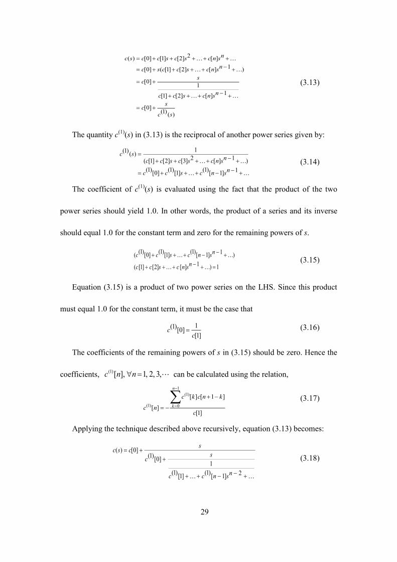
Table 3.3 Epsilon Table for Gregory’s π Series
1 0 1 2 3 4 5 6
0
4
0
-0.75
2.6667
3.1667
0
1.25
-28.75
3.4667
3.1333
3.1423
0
-1.75
82.25
-969.938
2.8952
3.1452
3.1413
3.1416
0
2.25
-177.75
3515.062
3.3397
3.1397
3.1416
0
-2.75
327.25
2.9760
3.1427
0
3.25
3.2837
The approximate value of π evaluated using the epsilon algorithm is the element
in the furthest even column. With 16 digits of precision, the value of π is evaluated as
3.141614906832299. The percent error in the value of π is 7.0834e-04%.
The percentage error in value of π obtained using different analytical continuation
techniques is found to be the same. Moreover, the value of π calculated using the
different procedures was numerically verified to be the exact up to 15 decimal places.
3.5.4 ACCELERATION OF CONVERGENCE OF π SERIES
The acceleration in the convergence of the series is best shown by comparing the
value of π obtained by directly summing the series against the value of obtained from
the Padé approximant (using the matrix method) with the same number of terms in the

39
series. It has been already established that the continued fraction and epsilon
algorithm are equivalent to the evaluating the Padé approximant. In
Table 3.4, the first column indicates the number of terms in the series. The
diagonal Padé approximant is evaluated using the matrix method and listed in the
second column. Columns 3 and 4 indicate the value of π obtained by evaluating the
Padé approximants and the power series respectively. The results are tabulated in
Table 3.4 with eight digits of precision. The numbers showed in bold are the
correct digits of π.
Table 3.4 Evaluating π using Padé Approximants with Matrix Method
Number
of terms
in series
Diagonal Padé
approximant
Diagonal Padé
evaluated at s=1
Truncated power
series
approximation
3 s
s
6.01
07.14
3.16666667 3.46666667
5 2
2
24.011.11
27.011.34
ss
ss
3.14234234 3.33968253
7 32
32
08.073.016.11
07.058.113.54
sss
sss
3.14161490 3.28373848
9 432
432
03.038.048.112.21
02.067.090.313.74
ssss
ssss
3.14159331 3.25236593
Graphically, the acceleration of convergence using the analytic continuation
techniques is shown in Figure 3.3. The value of π estimated by the power series and
Padé approximant is plotted against the number of terms in the series and compared
with the actual value of π.

40
Figure 3.3 Convergence of Power Series vs. Padé Approximant
From Figure 3.3, it is clearly seen that the convergence of the series can be
accelerated by the use of Padé approximants. For the same degree of accuracy as a [3/3]
Padé (calculated with 7 terms in the series), 31831 terms are required in the power
series approximation. While this example uses an extremely slowly converging power
series and while most gains are not this dramatic, this example gives a sense of what
can be achieved using Padé approximants.
The illustration of evaluating π shows that Padé approximants can be used to
accelerate slow converging series. It can also be used to evaluate certain ostensibly
diverging power series. More importantly, it can be used to evaluate the maximal
analytic continuation of the function as proved in Stahl’s theory [42], [43].

41
3.6 NUMERICAL ISSUES IN EVALUATING THE ANALYTIC
CONTINUATION
Numerical issues in evaluating an analytic function occur in
a) Calculation of power series coefficients of an analytic function.
b) Evaluating the analytic continuation of the power series.
The description of errors belonging to category a) can be subcategorized into the
following
i. Round-off errors: The calculation of power series coefficients in the PF problem
typically involves some form of convolution (as will be discussed in Chapter 4).
Round-off errors that occur during the calculation of one coefficient compound
in the calculation of the next coefficient and so on. Reference [20] suggests that
calculation of 40-60 terms in the series can exhaust the double precision
arithmetic due to round-off errors.
ii. Truncation errors: The power series approximation must be truncated to a finite
number of terms in order to calculate its analytic continuation. If sufficient
terms are not included in the series, the analytic continuation might not be an
accurate representation of the original function. The solution to this problem is
to add more terms in the series with appropriate consideration of the occurrence
of round-off errors and to the possibility that a solution might not exist to the
original equations.

42
The errors belonging to category b) are more relevant in this context and will be
discussed in detail with numerical examples later. The illustration of the numerical
issues is done using the matrix method of evaluating the Padé approximants. The other
methods of evaluating analytic continuation are also equally prone to such errors.
While implementing the different algorithms, their numerical performance should be
taken into account.
3.6.1 DEGENERATE POWER SERIES
The power series representation of an analytic function is said to be degenerate if it
leads to a singular matrix in calculation of the Padé approximants. Calculating the
denominator polynomial coefficients of the Padé approximant requires solving a linear
system of equations (3.11). The elements of the matrix in (3.11) depend on the
calculated coefficients of the power series. A degenerate series results in a singular
matrix with no solution. It is critical to be able to determine degenerate cases in the
numerical implementation of the Padé approximants to obtain reliable results.
A specific example of degeneracy occurs in the geometric series where the [L/2]
Padé approximants are degenerate for any value of L. A geometric series can arise out
of solving a simple scalar equation devoid of any complexities (viz. nonlinearity,
complex conjugate operation) using the holomorphic embedding procedure. Such
degeneracy can be illustrated using the following simple scalar linear equation,
bxa )1( (3.32)

43
where a, b are scalars. While the solution to the problem is trivial, solving this problem
in a manner that will be used for the nonlinear problem will help in understand the
numerical issues that can occur in the solution procedure.
To solve this problem, the variable x is expressed as a function of a complex parameter
s.
2]2[]1[]0[)( sxsxxsx (3.33)
From (3.32) a fixed-point form is established.
)()( saxbsx (3.34)
The equation is embedded with the complex parameter s such that at s=0 the solution is
known.
)()( sasxbsx (3.35)
The function x(s) is expanded and coefficients of like powers of s on both sides of the
equation are equated.
22 ]2[]1[]0[]2[]1[]0[ sxsxxasbsxsxx (3.36)
baaxx
abaxx
bx
2]1[]2[
]0[]1[
]0[
(3.37)
In general, the power series coefficients of the series x(s) can be expressed as:
bx ]0[
1,]1[][ nbanaxnxn
(3.38)
where x[n] denotes the coefficient of sn
in the power series.

44
The series x(s) to be evaluated for any arbitrary scalar a, b is
22)( bsaabsbsx (3.39)
From the calculated series coefficients, the evaluation of [L/2] Padé approximant
for an arbitrary value of L follows from (3.11) and (3.12).
]2[
]1[
]1[][
][]1[
1
2
Lx
Lx
b
b
LxLx
LxLx (3.40)
Substituting (3.38) in the above equation,
ba
ba
b
b
baba
babaL
L
LL
LL
2
1
1
2
1
1
(3.41)
The determinant of the LHS matrix is zero as shown in (3.42)
0
1
2221
2
21
1
1
aaba
aa
aba
baba
baba
L
L
LL
LL
(3.42)
Equation (3.42) shows that the Padé matrix for an [L/2] approximant turns out to be
singular for a geometric series resulting in no possible solution for the b coefficients. If
the coefficients are floating point numbers, the round-off error may prevent the matrix
from being exactly singular. However, the condition number of the Padé matrix will be
very high and the results obtained from any such calculation may be erroneous.
For this specific problem, it can be shown that the [0/1] Padé, as
bsx
1)( is an
exact representation of the solution. Evaluating the [L/2] Padé can be associated with
solving an over determined system of equations. It occurs due to specifying one too
many coefficients when it is not required. Hence, it becomes essential in the numerical

45
algorithm to recognize the cases where a smaller degree Padé approximant is sufficient
to accurately represent the power series.
3.6.2 ILL-CONDITIONED PADÉ MATRIX IN EVALUATING A
CONVERGENT SERIES
The power series coefficients of a convergent series, in most practical applications
do not become exactly zero for higher order terms. Due to floating point arithmetic
truncation and round-off errors in the calculation, the coefficients decrease
monotonically until they become small enough to be considered numerical zeros. In
such scenarios, evaluating a higher degree Padé means adding rows of numerical zeros,
that are nearly linearly dependent on each other to the Padé matrix (3.11), leading to a
very high condition number of the Padé matrix.
The following example of solving a two-bus dc PF problem from [46] results in a
convergent series and stands to illustrate the numerical issues associated with the Padé
matrix. Solving the quadratic equation that arises from the two-bus dc PF using HE is
demonstrated; it is then extended to the general ac PF problem in the next chapter.
P=0.09 p.u.
R=1 p.u.V1=1 p.u. V2=?
dc +-
Figure 3.4 Solving a dc PF problem using the HE procedure

46
The real power delivered at bus 2, P2, is related to the system voltages V1, V2 and the
line resistance R as follows:
0
)(
)(
12
2
2
2
12
212222
RPVVV
orV
RPVV
R
VVVIVP
(3.43)
For the system parameters in Figure 3.4, the expression is 009.02
2
2 VV . The
solution for this quadratic can be explicitly calculated as V2=0.9, 0.1 which are the HV
and LV solutions respectively. Now consider solving the simple quadratic using the
holomorphic embedding procedure. The receiving end voltage V2 is expressed as a
function of a complex parameter s. One possible embedding to calculate the HV
solution is:
2
2222
2
2
]2[]1[]0[)(,
)(
09.01)(
sVsVVsVwhere
sV
ssV
(3.44)
From the embedding it can be observed that the solution at s=0, V2(0) =1, is indeed
an operating solution under no-load conditions. This solution at s=0 is known as the
germ solution or, in short, germ; the HV solution is an analytic continuation of the germ
solution.
In calculating the voltage power-series coefficients from (3.44) a new series W2 (s)
is defined as the reciprocal of the voltage series.
2
222
2
2 ]2[]1[]0[)(
1)( sWsWW
sVsW (3.45)

47
The coefficients of the reciprocal series can be calculated using the relation that the
product of the two power series should yield 1.0. Thus, for the constant term,
]0[
1]0[
2
2V
W . It can be shown that, for a general value of n expanding (3.45) and
equating the coefficients of sn on LHS to zero yields:
1,]0[
][][
][2
1
0
22
2
nV
knVkW
nW
n
k (3.46)
From (3.44), substituting for 1/V2(s) with the reciprocal power series W2(s) yields:
2
222
2
222
]2[]1[]0[09.01
]2[]1[]0[
sWsWWs
sVsVV (3.47)
Equating the coefficients of s on both sides of (3.47) the power series coefficients
V2[n] can be calculated as:
1],1[09.0][
1]0[
22
2
nnWnV
V (3.48)
The power series evaluated using (3.46) and (3.48) is a convergent series whose
coefficients decrease monotonically.
32
2 0015.00081.009.1)( ssssV (3.49)
When evaluating a diagonal [M/M] Padé, coefficients up to s2M are required in the
series. As the degree of the Padé approximant needed in evaluating the series (3.49)
increases, the condition number of the matrix that arises from (3.24) for this particular
problem becomes larger. Recall that in solving the Ax=b problem, if the condition
number κ(A)=10k, up to k digits of precision could be lost [50]. While evaluating a

48
lower degree approximant may appear to be a potential solution to the problem, it may
lead to large truncation error in the solution.
Table 3.5 shows that for this particular convergent series, the condition number of
the Padé matrix increases up to the order of 1019
as the degree of the Padé approximant
increases. Thus, choosing an appropriate degree of the Padé approximant can involve a
tradeoff between the desired numerical stability properties as indicated by the condition
number and the allowable error tolerance in the solution. Also, the computational
complexity that is involved in obtaining a higher degree approximant should be taken
into consideration for practical applications.
Table 3.5 Condition Number of the Padé matrix used in Calculating the Padé
Approximant
Degree of Padé
approximant
Condition number of
Padé matrix
[2/2] 1.2548e+02
[4/4] 2.2891e+06
[6/6] 4.9530e+10
[8/8] 1.1808e+15
[10/10] 2.9682e+19

49
To summarize, this chapter discusses the relevance of analytic continuation in
solving the PF problem, illustrates different methods of evaluating the analytic
continuation with numerical examples and highlights the numerical issues that should
be taken into consideration.
50
4 SOLVING A GENERAL CASE POWER-FLOW PROBLEM WITH
HOLOMORPHIC EMBEDDING
4.1 INTRODUCTION TO HOLOMORPHIC EMBEDDING
Holomorphic functions form a branch of study in complex analysis. A brief
introduction about holomorphic functions followed by the development of load bus
model available in existing literature is presented in this section 4.1.
4.1.1 HOLOMORPHIC FUNCTIONS
Functions of complex variables that are complex differentiable everywhere in a
neighborhood around a point are said to be holomorphic about that point.
Holomorphic functions can be uniquely expressed using a convergent Taylor series in
the neighborhood of the point. The term ‘analytic’ is often used interchangeably with
‘holomorphic’. Analytic refers to a broader class of functions (real, complex or more
generic) that satisfy certain conditions whereas holomorphic refers to only complex
valued functions.
In real analysis, differentiability in a neighborhood does not guarantee analyticity;
however, in complex functions, differentiability in a neighborhood guarantees
analyticity. Analytic functions can be entire or non-entire. Functions whose Taylor
series expansion coincides with the actual function in the whole of the complex plane
are termed as entire. Examples of entire functions include trigonometric functions such
as sine, cosine and exponential function (ex). Entire functions have infinite radii of

51
convergence. For non-entire functions, the function can be expressed with a convergent
Taylor series only within an open disc of finite radius, centered about the point at which
the derivatives are calculated [38]. Analytic continuation techniques are employed to
extend the domain of convergence of such non-entire functions.
Holomorphic embedding (HE) as it is to be used here is the technique of
embedding the non-analytic PBE’s within a large problem with complex variables
ensuring that the resultant problem is holomorphic. For the PBE’s, the non-analyticity
(non-holomorphicity) is due to the complex conjugate operator. The solution
procedure for the load bus model using a particular embedding is shown in [21].
4.1.2 LOAD BUS MODELING USING HE
Consider the PBE of a load bus whose complex power injection Si is known. If m
were the set of PQ buses, the Power Balance Equation (PBE) for bus i, could be
expressed as,
miV
SVY
i
ik
N
k
ik
,*
*
1
(4.1)
where Yik is the (i, k) element of the bus admittance matrix, Si and Vi are the complex
power injection and voltage at bus i, respectively. The shunt elements in (4.1) are
moved to the RHS and the equation is embedded with a complex parameter s as
follows [21]:
misVsYsV
sSsVY ishunti
i
i
N
k
ktransik
,)()(
)(**
*
1
(4.2)

52
At s=1, the original PBE’s (4.1) are recovered from the embedded system of
equations, thereby retrieving the HV solution. In (4.2) Yik trans corresponds to the
“series branch” part of the admittance matrix. Consequently, the entries of each row
of the Yik trans matrix add up to zero; an exception is the row associated with nodes
adjacent to the slack bus. (Note that the embedded PBE for the slack bus is to be
introduced later and not included in (4.2).) The shunt admittance matrix, Yi shunt entries
model the shunt admittance components of the transmission line, off-nominal
transformer tap model, shunt capacitors/ reactors in the network.
With the parameter s as a variable, the notation V(s) is used to emphasize that the
voltage has become a holomorphic function of the complex parameter s. The complex
conjugate of the voltage, V* that appears in the PBE is replaced by, V
*(s
*) and not
V*(s). The presence of s
* rather than s in this term retains the property of
holomorphism and therefore analyticity. (More about this below.)
4.1.3 GERM SOLUTION FOR LOAD BUS MODEL
For solving the PF problem, a slack bus whose voltage magnitude and angle are
known is required. The defining equation for a slack bus is Vi=VispÐ0
o (iϵ slack)
where Visp
is the specified voltage magnitude at bus i. The complex power injection at
the slack bus is a free variable.
In (4.2), since the shunt elements are moved to the RHS and multiplied by s and
the complex power injections are also multiplied by s, the solution of (4.2) at s=0

53
corresponds to a network with no loads and no shunt element; hence all voltages are
identical to the slack bus voltage at s=0. It will be shown that it is convenient to use
the following model for the slack bus so that at s=0 the slack bus voltage is 1.0.
slackisVsV sp
ii ,)1(1)( (4.3)
In summary, for a system with only PQ buses, at s=0, all the shunt terms (Yi shunt)
and power injection (Si) in the PF equation (4.2) vanishes. This represents the
reference case where there is no generation and no load. In this case, (4.2) and (4.3)
reduce to
miVY
N
k
ktransik
,0)0(1
slackiVi ,1)0(
(4.4)
Equation (4.4) is a linear system of equations that could be solved to obtain the
germ solution. Since the entries of each row of the Yik trans matrix sum up to zero and
the slack bus voltage is 1.0, equation (4.4) holds good when all the bus voltages are
equal to 1Ð0o, which is called the germ solution. This is analogous to the flat start for
voltages in NR method.
In equation (4.4), if the slack bus equation were not included, the resulting Yik trans
matrix would be singular, leading to no possible solution for the germ. However, in
order to account for the slack bus, the entire row i, (∀ i=slack bus) in the Yik trans
matrix is zeroed, except the coefficient corresponding to Vslack. Hence the Yik trans
matrix is non-singular, resulting in a unique solution for the germ.

54
Since the voltage function as defined above is holomorphic (analytic), one
possible methodology of solving the problem (and the one used here) is to express
voltage as a power series, evaluate the coefficients of the power series and then
generate an analytic continuation of the series.
4.1.4 POWER SERIES EXPANSION
Embedding the PF equations such that the resulting equation is holomorphic
allows the voltage function to be represented by an equivalent power series. The
voltage function V(s) in (4.2) can be expressed as a Maclaurin series with s as the
expansion parameter.
0
)]([)(n
nsnVsV (4.5)
where the coefficients V[n] are complex numbers.
What follows is a proof of holomorphicity of the chosen embedding in (4.2) when
V(s) is expressed as a Maclaurin’s series. In particular, this justifies the usage of V*(s
*)
as opposed to V*(s) in the embedding.
In order to be holomorphic, a function must satisfy the Cauchy-Riemann
equations. An equivalent condition known as Wirtinger’s derivative requires that
0* sV [40]. i.e. The function V(s) should be independent of s* in order to be
holomorphic. The Maclaurin series expansion of the V*(s) (if it were to exist) and
V*(s
*), truncated at n terms are shown below:

55
n
n
snVsVVsV
snVsVVsV
][]1[]0[)(
][]1[]0[)(*****
******
(4.6)
In (4.6), the function V*(s) upon expansion has s
* terms on the RHS and
Wirtinger’s condition will not be satisfied. However, the expansion of V*(s
*)
independent of s* such that 0)( *** ssV . Thus the embedding (4.2) is
holomorphic only when the denominator in the RHS of (4.2) is chosen to be V*(s
*).
Assuming that we can represent the bus voltages as a Maclaurin series function of
s, that is Vi(s) and Vi*(s
*), we can substitute the series, (4.5) and (4.6), into (4.2) to
yield:
2
2***
*
1
2
]2[]1[]0[)]2[]1[]0[(
]2[]1[]0[
sVsVVsYsVsVV
sS
sVsVVY
iiishunti
iii
i
N
k
kkktransik
(4.7)
Our problem now is reduced to finding the series coefficients that satisfy (4.7). As
the first task it is recognized that in (4.7), the inverse of the voltage power series has
to be calculated. For every voltage function V(s), let W(s) be the new inverse power
series defined as 2]2[]1[]0[)( sWsWWsW . Since W(s) is the inverse of the V(s),
2]2[]1[]0[)(
1)( sWsWW
sVsW (4.8)
In order to calculate the coefficients of the inverse power series, (4.8) is multiplied
by V(s) on both sides.
1]2[]1[]0[]2[]1[]0[
1)()(
22
sVsVVsWsWW
sVsW (4.9)
By equating the coefficients of powers of s on both sides of the equation,

56
]0[
]1[]1[]2[]0[]2[0]0[]2[]1[]1[]2[]0[
]0[
]1[]0[]1[0]0[]1[]1[]0[
]0[
1]0[1]0[]0[
V
VWVWWVWVWVW
V
VWWVWVW
VWVW
(4.10)
In general, it can be written as:
1,]0[
][][
][
]0[
1]0[
1
0
nV
knVkW
nW
VW
n
k
(4.11)
It is to be remembered that in solving (4.7), for every series Vi(s), the inverse
series Wi(s) has to be calculated. Substituting equation (4.8) in (4.7):
2
2****
1
2
]2[]1[]0[
)]2[]1[]0[(
]2[]1[]0[
sVsVVsY
sWsWWsS
sVsVVY
iiishunti
iiii
N
k
kkktransik
(4.12)
Equating the coefficients of s, s2, s
3 … on both sides of (4.12) a recurrence
relation can be developed to solve for the power series coefficients. The general
expression for calculating the power series coefficients Vi[n] for n>0 can be obtained
as:
N
k
ishuntiiiktransik nVYnWSnVY
1
** ]1[]1[][ (4.13)
Equation (4.13) can be used to evaluate the coefficients of the voltage series for
load bus. In order to define a similar equation for slack bus, a special notation δni has
to be introduced.

57
otherwise
inifni
,0
,1 (4.14)
The term δni is associated with parameters that occur only for the powers of s raised
to i and vanish for the remaining powers of s. Thus, from the slack bus equation defined
in (4.3), an expression for the power series coefficients can be written as:
slackiVnVsp
inni ),1(][ 10 (4.15)
Remember that the solution for n=0 is the germ solution, where all bus voltages
are 1Ð0o. By knowing the V and W series up to (n-1) coefficients, the n
th coefficient
of the voltage power series can be calculated from (4.13) and (4.15) by solving a
linear matrix equation. The coefficients of inverse series Wi up to n coefficients can be
obtained from the voltage series up to n coefficients from (4.11). Thus by evaluating
the appropriate germ solution at s=0, the entire voltage power series up to the desired
number of terms can be constructed from (4.13). The power series obtained thus,
evaluated at s=1, will give the required voltage solution. If the radius of convergence
of the any of the voltage series is less than 1.0, the power series will not converge by
itself to the desired solution. The radius of convergence is generally unknown; hence,
the property of analytic continuation is employed to represent the powers series within
and beyond its radius of convergence and evaluate the voltage solution.
4.2 GENERATOR BUS MODEL I USING HOLOMORPHIC EMBEDDING
Current literature does not contain a holomorphically embedded equation for
modeling the generator bus. In PF studies, generator / PV / voltage bus refers to a bus

58
in which the voltage is to be held at a constant value. The reactive power capability of
the generator is a limiting factor in maintaining a constant bus voltage magnitude.
Therefore, for a generator bus, the voltage magnitude and real power output are
known quantities while voltage angle and reactive power are unknown.
The traditional defining equations for a PV bus i, are:
piVYVP
N
k
kikii
,)Re(1
** (4.16)
piVVsp
ii , (4.17)
where Pi denotes the real power injection and Visp
the voltage magnitude at bus i.
The reactive power being a variable is a significant difference between the
generator bus and the load bus models. Two different approaches for handling the
reactive power term in the PBE’s are studied. In the first approach, the reactive power
term is made a free variable, represented as a function of the complex s parameter. A
second approach is to eliminate the reactive power term by summing the complex
power and it’s conjugate. Both approaches are developed in detail and used in solving
the general case PF problem. Described in this section is the first PV bus model.
Generator bus model I involves modeling the unknown reactive power injection as
a holomorphic function in the s parameter [52]. The voltage magnitude constraint of
the generator bus is also embedded, with the bus voltage defined as a holomorphic
function. This section presents the PV bus formulation for a N-bus system and
demonstrates the calculation of the power series coefficients. The numerical

59
implementation of the formulation requires breaking the equation into real and
imaginary parts.
For the N-bus system, let p denote the set of PV buses. The complex PBE’s for a
generator bus iϵp, with the reactive power, Q, represented as a holomorphic function
is:
pisVYsV
sjQsPsVY ishunti
i
ii
N
k
ktransik
,)()(
)()(
**
1
(4.18)
In (4.18), an additional free variable Qi(s) is introduced. It is important to note that
unlike the voltage power series that can have complex coefficients, the reactive power
series has only real coefficients.
Inclusion of a free variable in the generator bus model requires an additional
constraint. For the generator bus, we have the voltage magnitude constraint (4.17).
Equation (4.17) can be embedded in the complex parameter s as shown below:
piVssVsVsp
iii
,11)()(
2**
(4.19)
Evaluating (4.19) at s=1, the voltage magnitude constraint of the generator bus
can be retrieved. Equations (4.18) and (4.19) represent the HE formulation for the
generator bus model.
For a problem with N buses, the HE system of equations that describe the different
bus types are shown in equations (4.2), (4.3), (4.18) and (4.19). The original PBE’s
and their counterpart holomorphically embedded equations for each type of bus are
summarized from the above listed equations in Table 4.1.
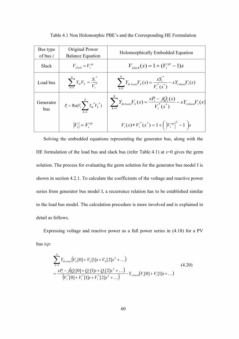
60
Table 4.1 Non Holomorphic PBE’s and the Corresponding HE Formulation
Bus type
of bus i
Original Power
Balance Equation Holomorphically Embedded Equation
Slack sp
islack VV sVsV sp
islack )1(1)(
Load bus *
*
1 i
ik
N
k
ikV
SVY
)()(
)(**
*
1
sVsYsV
sSsVY ishunti
i
i
N
k
ktransik
Generator
bus )Re(
1
**
N
k
kikii VYVP )(
)(
)()(
**
1
sVsYsV
sjQsPsVY ishunti
i
ii
N
k
ktransik
sp
ii VV sVsVsV sp
iii
11)()(
2**
Solving the embedded equations representing the generator bus, along with the
HE formulation of the load bus and slack bus (refer Table 4.1) at s=0 gives the germ
solution. The process for evaluating the germ solution for the generator bus model I is
shown in section 4.2.1. To calculate the coefficients of the voltage and reactive power
series from generator bus model I, a recurrence relation has to be established similar
to the load bus model. The calculation procedure is more involved and is explained in
detail as follows.
Expressing voltage and reactive power as a full power series in (4.18) for a PV
bus iϵp:
sVVYsVsVV
sQsQQjsP
sVsVVY
iishunti
iii
iiii
N
k
kkktransik
]1[]0[]2[]1[]0[
]2[]1[]0[
]2[]1[]0[
2***
2
1
2
(4.20)

61
An inverse function Wi(s) is defined to be reciprocal of the voltage power series
for bus i. The definition of the inverse series, calculation of its coefficients is identical
to the load bus model described by the equations (4.8) - (4.11). Thus (4.20) becomes
sVVY
sWsWWsQsQQjsP
sVsVVY
iishunti
iiiiiii
N
k
kkktransik
]1[]0[
]2[]1[]0[]2[]1[]0[
]2[]1[]0[
2***2
1
2
(4.21)
Equating the coefficients of s, s2 and so on up to s
n,
]1[][][]1[][
]1[]0[]2[]1[]1[]2[]0[]1[]2[
]0[]0[]1[]1[]0[]0[]1[
0
**
1
****
1
***
1
nVYknWkQjnWPnVY
VYWQWQWQjWPVY
VYWQWQjWPVY
ishunti
n
k
iiii
N
k
kik
ishuntiiiiiiiii
N
k
kik
ishuntiiiiiii
N
k
kik
(4.22)
In (4.22), the calculation of the voltage series coefficients Vi[n] involves the sum
of product of two power series coefficients Qi, Wi (the
n
k
ii knWkQ0
*][][ term) which
can be expanded as:
]0[][]2[]2[]1[]1[][]0[
][][
****
0
*
iiiiiiii
n
k
ii
WnQnWQnWQnWQ
knWkQ
(4.23)
Observe from (4.22) and (4.23) that in calculating of the nth
order coefficient of the
voltage power series (i.e. Vi[n]), both the nth
order coefficients of the W series and the Q
series (Wi[n], Qi[n]) are required. Recall, the calculation of Wi[n] requires the Vi[n] term
from (4.11) whereas calculating Vi[n] was the objective to begin with. This scenario is

62
unlike the load bus model where the nth
coefficient of the power series could be
expressed in terms of coefficients up to the degree n-1.
From (4.23), a linear recurrence relationship to calculate the power series
coefficients has to be developed. A two-part solution is devised to achieve this.
i. The germ solution of the voltage and reactive power series is determined
and used to simplify (4.22).
ii. The voltage power series is broken down into real and imaginary
coefficients when enforcing the voltage magnitude constraint and real
power constraint of the generator bus model.
The implementation details of the above-suggestions in determining the germ
solution and power series coefficients of the generator bus model are shown in the
following sections.
4.2.1 GERM SOLUTION FOR THE GENERATOR BUS MODEL I
To obtain the germ solution of the PV bus model in a general PF problem, the HE
equations corresponding to load bus (equation (4.2)), generator bus (equations (4.18)
and (4.19)) and slack bus (equation (4.3)) have to be solved simultaneously at s=0. At
s=0, the system of equations listed above becomes:
slackiV
pii
Vi
V
piV
jQVY
miVY
i
i
i
N
k
ktransik
N
k
ktransik
,1)0(
,1)0(*)0(
,)0(
)0()0(
,0)0(
*
1
1
(4.24)

63
In (4.24), the slack bus voltage is known to be 1.0. If the germ solution for the
remaining bus voltages were chosen to be 1.0, the load bus equation in (4.24) would
be satisfied (refer discussion in Section 4.1.3); the generator voltage magnitude
constraint in (4.24) will also be met, since the product Vi(0) Vi*(0) would equal 1.0.
The embedded generator power balance constraint (4.24), however, has a variable
Qi(0) on the RHS of (4.24). Substituting the assumed germ voltage solution of 1.0 for
all buses in (4.24), the embedded generator bus PBE becomes:
piQ
pijQ
piV
jQsVY
i
i
i
i
N
k
ktransik
,0)0(
,1
)0(0
,)0(
)0()(
*
1
(4.25)
If the reactive power germ, Qi(0) (∀ iϵp) were chosen to be 0.0 (from (4.25)) and
all bus voltages were equal to 1.0, the embedded system of equations for all bus types
at s=0; (equation (4.24)) are satisfied. Hence, Vi(0)=1, Qi(0)=0 is chosen to be the
germ solution to the embedded system of equations presented in (4.2), (4.3), (4.18)
and (4.19). It is also the physical solution for the no-load, no-generation case for a
general PF problem when there are no shunts and the generator bus voltages are
maintained at 1.0. The calculated germ solution, Vi(0) and Qi(0) also represent the
constant term (coefficient of s0 term) in the power series, Vi[0] and Qi[0], respectively,
for generator bus model I.

64
4.2.2 EVALUATING POWER SERIES COEFFICIENTS FOR GENERATOR
BUS MODEL I
With the particular choice of embedding for the generator bus model as shown in
(4.18) and (4.19), the calculation of the germ solution was demonstrated in Section
4.2.1. This subsection shows the procedure of calculating the remaining power series
coefficients.
Rewriting (4.22) derived from the power balance constraint of the generator bus
model, with the new evaluated germ Qi[0]=0, Wi[0]=1/Vi[0]=1 yields.
]1[][][][]1[
][
1
1
**
1
nVYnQknWkQjnWP
nVY
iishunti
n
k
iiii
N
k
ktransik
(4.26)
A new quantity Rhs_Known[n-1] is introduced to make the equation succinct in
the subsequent steps. Rhs_Known[n-1] denotes the quantities in the RHS of (4.26)
with coefficients up to degree n-1.
]1[][][]1[
]1[_
1
1
**
nVYknWkQjnWP
nKnownRhs
iishunt
n
k
iiii
(4.27)
Substituting(4.27), equation (4.26)becomes,
][]1[_][
1
njQnKnownRhsnVY i
N
k
ktransik
(4.28)
Equation (4.28), which was derived from the embedded PBE of the generator bus,
(4.18), defines a recurrence relation that is used in calculating the voltage series
coefficients and reactive power series coefficients. A similar equation needs to be

65
derived from the voltage magnitude constraint of the generator bus, (4.19). Expressing
the voltage function Vi(s) as power series in equation (4.19) yields:
sV
sVsVVsVsVV
spi
iiiiii
11
]2[]1[]0[]2[]1[]0[
2
2***2 (4.29)
Equating the coefficients of powers of s on both sides yields,
]1[]2[]2[]1[]3[2]3[]3[
0]0[]3[]1[]2[]2[]1[]3[]0[
]1[]1[]2[2]2[]2[
0]0[]2[]1[]1[]2[]0[
1]1[2]1[]1[
1]0[]1[]1[]0[
)(1]0[
1]0[]0[
***
****
**
***
2*
2**
*
iiiireiii
iiiiiiii
iireiii
iiiiii
spireiii
spiiiii
i
ii
VVVVVVV
VVVVVVVV
VVVVV
VVVVVV
VVVV
VVVVV
solutiongermV
VV
(4.30)
In (4.30) Vi re[n] represents the real part of the voltage power series nth coefficient
from the voltage magnitude constraint. The notation δni as defined in (4.14) is used to
write a generalized expression to evaluate Vi re[n].The calculation of Vi re[n] for an
arbitrary value of n, can be written from (4.30) as,
1
1
*
2
10 ][][2
1
2
1][
n
k
ii
spi
nnrei knVkVV
nV (4.31)
Equations (4.26) and (4.31) represent a consistent system of equations
representing the generator bus model that has a unique solution. However, the
solution of the equations is not trivial in their current form since there are unknowns
on both sides of (4.26). The objective is to rearrange the equations so that the power

66
series coefficients can be obtained by solving a single linear matrix equation. It is
achieved by breaking the complex voltage power series coefficients into real and
imaginary parts. While this is necessary for solving the generator bus power series
coefficients, it becomes inevitable in the implementation that the load bus power
series coefficients are also broken down into real and imaginary components since the
system of equations are mutually coupled. Let the entries of the admittance matrix
(without shunt elements) be expressed as ikiktransik jBGY . The voltage series
coefficients are broken into real and imaginary parts ][][][ njVnVnV imireii . Thus,
the LHS of (4.26) is alternatively expressed for every bus i as follows:
N
k
imkikrekikimkikrekik
N
k
imkrekikik
N
k
ktransik
nVGnVBjnVBnVG
njVnVjBGnVY
1
11
][][][][
][][][
(4.32)
The holomorphically embedded PV bus equation (4.26) for bus i as broken into
real and imaginary components is represented as a matrix equation below. The
quantities that can be evaluated on the RHS (involves coefficients up to sn-1
) are
represented using the term Rhs_Known defined in (4.27).

67
][])1[_Im(
])1[_Re(
][
][
][
][
][
][
1
1
11
11
nQnKnownRhs
nKnownRhs
nV
nV
nV
nV
nV
nV
GBGBGB
BGBGBG
i
imN
reN
imi
rei
im
re
iNiNiiiiii
iNiNiiiiii
(4.33)
In calculating the nth
degree voltage power series coefficients, the quantity Vi re[n]
can be calculated for all voltage buses iϵp, from the voltage magnitude constraint
(4.31). However, Qi[n] shown in the RHS of (4.33) is still unknown. This is similar to
solving the Ax=b problem with a few of the x’s known beforehand but the same
number of b’s as unknowns. Such problems can be solved by bringing all the
unknowns to the LHS and known quantities to the RHS.
To do this, the product of the known Vi re[n] coefficient and corresponding column
vector of the LHS matrix is moved to the RHS. For a PV bus, i, the matrix equation
(4.33) thus becomes:
][])1[_Im(
])1[_Re(
][
][
][
][
][
][
1
0
1
1
11
11
nVB
G
nKnownRhs
nKnownRhs
nV
nV
nV
nQ
nV
nV
GBGGB
BGBBG
reiii
ii
imN
reN
imi
i
im
re
iNiNiiii
iNiNiiii
(4.34)
68
Equation (4.34) represents the recurrence relation for one generator bus i. When
the PBE’s for a N bus system are listed, the coefficients of the LHS matrix and RHS
vector for the remaining buses have to be altered, to account for moving unknown
variables to LHS and known variables to RHS. To demonstrate this, a sample
three-bus system with a PV bus is chosen; the recurrence relation with unknowns on
both sides of the equation is shown first. Subsequently, the alteration in the matrix and
RHS vector entries is shown. The concept can be generalized for a N-bus system.
Figure 4.1 shows a sample three-bus problem where bus 1 is the slack bus; bus 2
is the generator bus and bus 3 is the load bus.
1
3
2
Figure 4.1 Sample Three-bus Test System
In order to write the recurrence relation, as a matrix equation, (4.13), (4.15), (4.31)
and (4.33) are to be referred to and combined appropriately. The definition for each
entry in the matrix equation is available in the nomenclature. The matrix equation for

69
different bus types combined is shown in (4.35); for PV bus 2, unknowns Vi im[n] and
Qi[n] exist on both sides of the equation.
1
1
*222
1
2
2102
33*
3*3
33*
3*3
2
10
3
3
2
2
1
1
333332323131
333332323131
232322222121
232322222121
][][2
1][
])1[]1[Im(
])1[]1[Re(
][])1[_Im(
])1[_Re(
0
1
][
][
][
][
][
][
1
1
n
k
sp
nnre
shunt
shunt
Slacknn
im
re
im
re
im
re
knVkVV
nV
nVYnWS
nVYnWS
nQnKnownRhs
nKnownRhs
V
nV
nV
nV
nV
nV
nV
GBGBGB
BGBGBG
GBGBGB
BGBGBG
(4.35)
In (4.35), the value of V2 re[n] can be calculated from the voltage magnitude
constraint. The vector resulting from the product of column 3 (the column
corresponding to entry V2 re[n]) and the known value of V2 re[n] is moved to the RHS.
The unknown Q2[n] is moved to the LHS unknown vector, in place of V2 re[n]; the
LHS matrix entries are altered by zeroing the coefficients corresponding to Q2[n] in
all equations, except equation 4 (equation (4.34)). The equations from (4.35) are
altered as:
1
1
*222
1
2
2102
2
32
32
22
22
33*
3*3
33*
3*3
10
3
3
2
2
1
1
3333323131
3333323131
2323222121
2323222121
][][2
1][
][
0
0
])1[]1[Im(
])1[]1[Re(
])1[_Im(
])1[_Re(
0
1
][
][
][
][
][
][
0
0
1
0
1
1
n
k
sp
nnre
re
shunt
shunt
Slacknn
im
re
im
im
re
knVkVV
nV
nV
B
G
B
G
nVYnWS
nVYnWS
nKnownRhs
nKnownRhs
V
nV
nV
nV
nQ
nV
nV
GBGGB
BGBBG
GBGGB
BGBBG
(4.36)
The matrix on the LHS of (4.36) is constructed by breaking the Yik trans matrix into
real and imaginary components and correcting the coefficients corresponding to slack
bus and PV buses; from here on, the matrix will be referred as iteration matrix. From
70
(4.36), it can be observed that the iteration matrix is not incident symmetric; also it
loses the property of diagonal dominance. Hence, a LU factorization technique with
pivoting has been used to solve the linear matrix problem and obtain the power series
coefficients; however, no attempt has been made to determine whether there is an
ordering to the equations where pivoting is not needed.
These equations from (3.46), for different RHS n indices are solved repeatedly until
the desired number of terms in the power series is calculated. The analytic continuation
of the voltage power series from the calculated coefficients is evaluated using Padé
approximants. A numerical example demonstrating the implementation of generator
bus model I is presented in Section 4.5.
4.3 GENERATOR BUS MODEL II USING HE
In the above PV bus formulation, the reactive power term was expressed as a
holomorphic function in the s parameter. Another way of representing the generator
bus model is eliminating the reactive power term by summing the complex power and
its conjugate as shown in [51].
The traditional defining equations for a PV bus, i, are shown in (4.16) and (4.17).
Unlike the PQ bus where complex equality constraints are used, for the PV bus
equality constraints needed are only on the real part of the complex power injection.
Real power injection, Pi, from (4.16) can be expressed in terms of complex power, Si
and subsequently in terms of bus voltages, Vi and bus admittance matrix, Yik, as
follows:

71
N
k
ikiki
N
k
kiki
iii
PVYVVYV
PSS
1
*
1
**
*
2)()(
2
(4.37)
The bus admittance matrix can be separated into its series branch part and shunt
admittance component as follows:
iiishunti
N
k
ktransiki
N
k
ktransiki
ishuntishuntiii
N
k
ktransiki
N
k
ktransiki
N
k
iishuntiiktransiki
ishuntii
N
k
ktransiki
PVVYVYVVYV
PYYVVVYVVYV
PVYVVYV
VYVVYV
2)Re(2)()(
2)()()(
2)()(
)()(
*
1
*
1
**
**
1
*
1
**
1
**
**
1
**
(4.38)
The network shunt elements from the shunt admittance of transmission lines,
transformer taps, shunt reactors and shunt capacitors, which contribute to the diagonal
values of the bus admittance matrix, do not affect the real power injection. This is due
to the cancellation of the imaginary component in the Yi shunt+ Yi shunt* term. However,
real power is affected by the real component of the Yi shunt term; for example by shunt
conductance modeling the corona losses. In developing the generator bus model II
using HE, for simplicity, the shunt conductance is not accommodated; hence, the
2Re(Yi shunt)ViVi* term in (4.38) is not modeled. The resulting expression from (4.38) is
embedded in the complex parameter s yielding:
N
k
iktransiki
N
k
ktransiki sPsVYsVsVYsV
1
**
1
***2))()(())()(( (4.39)

72
The voltage magnitude constraint is holomorphically embedded as:
pissp
iVsVs
iV i
,1
21)(*)( **
(4.40)
Solving (4.39) and (4.40) at s=0 while expressing the voltage function as a power
series (refer to (4.5)), the system of equations for the PV bus, i, reduces to
N
k
ktransiki
N
k
ktransiki VYVVYV1
*
1
**0])0[]0[()]0[]0[(
1]0[*]0[ * iVi
V
(4.41)
To obtain the germ solution when using this PV bus model, the s=0 equations
representing the load bus and slack bus have to be solved with (4.41) simultaneously.
From equation (4.24) the equations representing the load bus and slack bus at s=0 are:
slackiV
miVY
i
N
k
ktransik
,1]0[
,0]0[1
(4.42)
If the germ solution for all bus voltages, (i.e. Vi[0]) is 1Ð0o, the terms
N
k
ktransik VY1
**]0[ ,
N
k
ktransik VY1
]0[ in equation (4.41) evaluate to be zero; the reason
being the diagonal element in Yik trans matrix is the negative sum of the off-diagonal
elements. Also, the voltage magnitude constraint is satisfied at s=0. It has been
established from Section 4.2.1 that the germ solution of bus voltages equal to 1Ð0o
satisfies (4.42). Thus, the unique germ solution for the voltage function for this
holomorphic embedding with generator bus model II must be 1Ð0o for all buses.

73
4.3.1 EVALUATING THE VOLTAGE SERIES COEFFICIENTS FOR
GENERATOR BUS MODEL II
A recurrence relation that expresses the nth
degree coefficients of the voltage series
as a function of (n-1) coefficients is next established for this PV bus model, along with
the PQ bus model describe earlier. First, the voltage function is represented with a
power series truncated up to sn
terms. Next, the voltage series and admittance bus
entries are broken into real and imaginary components. The entries of the admittance
matrix (without shunt elements) are expressed as . The voltage
series coefficients are broken into real and imaginary parts .
The equations resulting from the expansion of the terms ))()((
1
***
N
k
ktransiki sVYsV and
N
k
ktransiki sVYsV1
**))()(( are shown in equations (4.43)-(4.52). For a PV bus i, the latter
term is expanded as:
N
k
nimkrekimkrekikik
nimireiimireiimirei
N
k
nkkktransik
niii
N
k
ktransiki
snjVnVjVVjBG
snjVnVsjVVjVV
snVsVVYsnVsVV
sVYsV
1
1
***
1
**
][][]0[]0[
][][]1[]1[]0[]0[
][]1[]0[][]1[]0[
)()(
(4.43)
Since there is a product of two power series in (4.43), the coefficient of sn is the
sum of the products of the coefficients whose powers of s add up to n. To illustrate the
ikiktransik jBGY
][][][ njVnVnV imireii
74
above statement, consider two series a(s), b(s) and their product c(s) defined as
follows:
00
][)(,][)(n
n
n
n snbsbsnasa
0
][)()()(n
nsncsbsasc
(4.44)
The coefficient of the series c[n] is related to the coefficients a[n], b[n] as:
nyx
nyxybxanc ,0],[][][ (4.45)
The equation (4.43) involves the product of two power series. Applying the same
principle discussed above, the sn th
term of the series in (4.43) is:
nyx
syjVyVjBGsxjVxVnyx
N
k
y
imkrekikik
x
imirei
,0
][][][][1
(4.46)
The coefficient of sn
is then expressed in terms of real variables by carefully
performing the complex arithmetic from (4.46). The real and imaginary part of the
complex equation derived from (4.46) is:
][
][
][
][][][
1yV
yVGBj
yV
yVBGxjVxV
imk
rek
ikik
imk
rekN
k
ikik
nyx
imirei
nyx imk
rekN
k
imiikreiikimiikreiik
nyx imk
rekN
k
imiikreiikimiikreiik
yV
yVxVBxVGxVGxVBj
yV
yVxVGxVBxVBxVG
][
][][][][][
][
][][][][][
1
1
(4.47)
75
Equations (4.43)-(4.47) represent the expansion of the
N
k
ktransiki sVYsV1
**)()(
term in (4.39). The ))()((1
***
N
k
ktransiki sVYsV term can be expanded similarly resulting
in the following term.
nyx imk
rekN
k
imiikreiikimiikreiik
nyx imk
rekN
k
imiikreiikimiikreiik
yV
yVxVBxVGxVGxVBj
yV
yVxVGxVBxVBxVG
][
][][][][][
][
][][][][][
1
1
(4.48)
Equations (4.47) and (4.48) are expanded forms of the individual terms present in
LHS of equation (4.39). From equations (4.47) and (4.48) it can be observed that the
coefficients on the real components are the same; the coefficients of the imaginary
components are opposite in sign and add up to zero. The original equation to begin with
was the real power constraint; hence, imaginary coefficients adding up to zero is
expected. Upon adding the coefficients of (4.47) and (4.48), the sum becomes:
nyx imk
rekN
k
imiikreiikimiikreiik yV
yVxVGxVBxVBxVG
][
][][][][][2
1
(4.49)
The objective now is to express the calculation of power series coefficients of order
n (Vi re[n] and Vi im[n]), using a linear matrix equation. Hence, the unknown quantities
(Vi re[n] and Vi im[n]) will be retained on the LHS; the known quantities (coefficients
up to degree n-1) will be moved to the RHS. (More about this below in the discussion
regarding calculating the RHS term). Calculating the coefficients of sn
, n≥0 from (4.49),
the unknown coefficients, Vk re[n] and Vk im[n], occur only when x=0, y=n and x=n,

76
y=0; In other words, the unknown coefficients occur in only two of the n+1 terms that
meet the relation x+y=n, x, y >0. These are:
]0[
]0[][][][][2
][
][]0[]0[]0[]0[2
1
1
imk
rekN
k
imiikreiikimiikreiik
imk
rekN
k
imiikreiikimiikreiik
V
VnVGnVBnVBnVG
nV
nVVGVBVBVG
(4.50)
As a part of expressing the calculation process as a linear matrix equation, (4.50)
is to be expressed as a product of a known row vector (which will become part of a
larger iteration matrix) and an unknown column vector of voltage series terms, Vk re[n]
and Vk im[n] ∀ values of k. For succinct representation of the iteration matrix entries,
the coefficients of the elements Vk re[n] and Vk im[n] are denoted by γik and βik
respectively where i is the index of the generator bus whose real power balance
constraint is being modeled. The coefficients γik and βik for k≠i can be derived from
(4.50) as:
ikVGVB
ikVBVG
imiikreiikik
imiikreiikik
,]0[]0[2
,]0[]0[2
(4.51)
The coefficients of Vi re[n], Vi im[n] for a PV bus, i, aggregated from (4.50) are,
N
k
imkikrekikimiiireiiiii
N
k
imkikrekikimiiireiiiii
VGVBVGVB
VBVGVBVG
1
1
]0[]0[]0[]0[2
]0[]0[]0[]0[2
(4.52)
Equations (4.51) and (4.52) represent the coefficients of the unknown power
series terms Vi re[n] and Vi im[n]; they are derived from the real power constraint of

77
generator bus i; they constitute the entries of the iteration matrix used to determine the
power series coefficients.
The RHS of the real power constraint in the voltage bus model, from (4.39) occurs
only for power of s raised to one. Hence, the term δn1 (as defined in (4.14)) is
multiplied with the real power injection term 2Pi. Also, recall from (4.48) that only the
coefficients of sn
(occurring for xnynxx &,0 ) are retained on the LHS. The
remaining coefficients ( xnynx &1,2,1 ) are known and can be moved to
the RHS of the equation corresponding to the real power constraint. Thus, the RHS
element corresponding to the real power constraint for a PV bus, i, denoted by the
term ζi[n], can be expressed for a general value of n as:
1
1 1
1 ][
][][][][][2][
n
x
N
kimk
rek
imiikreiikimiikreiikini xnV
xnVxVGxVBxVBxVGPn (4.53)
The voltage magnitude constraint for a generator bus remains the same as shown
in Section 4.2.2 from equations (4.29)-(4.31). The expression for a real coefficient in
the voltage series Vi re[n] is derived from the embedded voltage magnitude constraint.
1
1
*
2
10 ][][2
1
2
1][
n
k
ii
sp
innrei knVkV
VnV (4.54)
When (4.54) is to be represented in the matrix equation, the entry corresponding
to Vi re[n] is made one; the remaining elements of the particular row in the LHS matrix
are zeroed.

78
To summarize, for every PV bus. i, equations (4.51), (4.52) represent the LHS
coefficients that correspond to the real power constraint; equation (4.53) is the RHS
term corresponding to the real power constraint; and equation (4.54) corresponds to
the voltage magnitude constraint for the PV bus, i. The unknowns are the real and
imaginary nth
series coefficients of the voltage series. Thus, the HE generator bus
model obtained by eliminating the reactive power term, can be represented with a
linear system of equations that has a unique solution. The primary difference from the
previously described model is the equations used to represent the real power
constraint of generator buses. Another difference is that the reactive power generated
by PV bus i, QGi has to be evaluated from the calculated voltage solution, the network
parameters and reactive power loading data.
To compare the difference in the structure of the equations that result from
implementing generator bus model I against model II, the three-bus example shown in
Figure 4.1 is considered. The slack bus and load bus are represented by HE defined in
equations (4.2) and (4.3). The generator bus is represented by the HE presented in
equations (4.39) and (4.40). The calculation of the voltage series coefficients for the
three-bus problem can be expressed using a linear matrix equation shown below
])1[]1[Im(
])1[]1[Re(
][][2
1
][
0
1
][
][
][
][
][
][
1
1
1
33*
3*3
33*
3*3
1
1
*222
1
2
210
2
10
3
3
2
2
1
1
333332323131
333332323131
232322222121
nVYnWS
nVYnWS
knVkVV
n
V
nV
nV
nV
nV
nV
nV
GBGBGB
BGBGBG
shunt
shunt
n
k
sp
nn
Slacknn
im
re
im
re
im
re
(4.55)

79
In (4.55), the equations representing the slack bus (rows 1 and 2) and the load bus
(rows 5 and 6) remain unaltered from (4.36). Equations representing generator bus
model (rows 3 and 4) are modified based on equations (4.51)-(4.54). The voltage
power series coefficients can be obtained by repeatedly solving (4.55). The remaining
procedure involved in calculating the bus voltages such as usage of analytic
continuation, convergence criteria described in Section 4.2 is still applicable.
4.4 POWER-FLOW SOLUTION USING HE
The above described generator bus models do not incorporate the reactive power
limit of generators. A physical limit on equipment introduces discontinuities in the
problem. This section describes the handling of reactive power limits on generators,
discusses the convergence criteria and presents a flow chart for solving the PF
problem using the HE procedure.
4.4.1 HANDLING REACTIVE POWER LIMITS OF GENERATOR
Currently, the reactive power limits of generator are handled in the power flow
program as follows. Let QGi MIN, QGi MAX represent the minimum and maximum
reactive power limits on generator at bus i respectively. The germ solution followed
by a fixed number of terms (say 5) of the power series coefficients are calculated
using the HE procedure. For PV bus model I, the analytic continuation of the reactive
power series Qi(s) gives the reactive power injection required to maintain the voltage
to the specified value at bus i. Any reactive power load at bus i is added to obtain the

80
total reactive power generated, QGi. For the PV bus model II, the QGi value is
evaluated from the calculated bus voltages.
If the reactive power limits of the limits are violated (QGi > QGi MAX or QGi <
QGiMIN), the bus type is changed from PV bus to PQ bus. Depending on the maximum
or minimum limit that is violated, the reactive power generation at the buses is chosen
to be QGi MAX or QGi MIN. Now, the reactive power injection at the buses is known and
the voltage magnitude becomes a free variable. Hence, the buses are represented using
the load bus equations described in Section 4.1. The PF problem is re-solved with the
altered bus types. This involves recalculating the iteration matrix and establishing a
recurrence relation to evaluate the power series coefficients using the altered bus
types. The power series coefficients are calculated up to any desired order. From the
analytic continuation of the series thus obtained, i.e., the candidate solution, the
violation of generator capability is checked. Any additional violation of the reactive
power limits or regaining control of PV buses requires resolving the problem again.
Table 4.2 Listing of Bus Types in the PF Problem
Bus type
index
Bus type
description
Known
variables
Unknown
variables
0 PQ P,Q |V|,θ
2 PV P,|V| Q, θ
3 Slack |V|,θ P,Q
4 PV on minimum Q limit P,Q |V|,θ
5 PV bus on maximum Q limit P,Q |V|,θ

81
Based on whether the maximum or minimum reactive power limit is violated a
different bus type is assigned. The list of bus type, the indices used to identify the bus
types and the corresponding known and unknown variables are listed in Table 4.2.
4.4.2 CONVERGENCE CRITERIA
In the implementation of the HE method, only a finite number of terms in the
voltage series are calculated. The number of terms required in the voltage series to find
a converged solution varies from problem to problem. Either of the following
conditions can be used to determine convergence and end the calculation of the power
series.
1. The change in the voltage solution is less than a specified tolerance.
2. The mismatch in the original PBE’s is less than a tolerance value
In our implementation of the HE method, the convergence criteria was chosen to be
the mismatch in the original defining equations of each bus type, i.e. complex power
injection for load buses (4.1), real power injection and voltage magnitude for generator
buses (equations(4.16) and (4.17)). The maximum allowable tolerance for the
mismatch (ΔP, ΔQ for PQ buses and ΔP, Δ|V| for PV buses) was taken as 1e-04 p.u.
4.4.3 FLOWCHART
The procedure for solving the PF problem with reactive power limits on generators
using the HE procedure is shown in Figure 4.2.
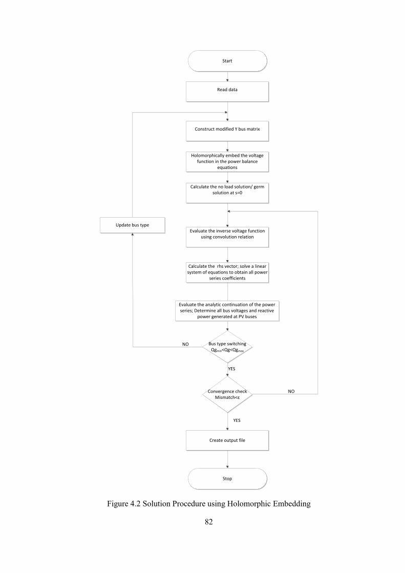
82
Read data
Construct modified Y bus matrix
Holomorphically embed the voltage function in the power balance
equations
Calculate the no load solution/ germ solution at s=0
Evaluate the inverse voltage function using convolution relation
Calculate the rhs vector; solve a linear system of equations to obtain all power
series coefficients
Create output file
Bus type switchingQgmin<Qg<Qgmax
Convergence checkMismatch<ε
Stop
Start
YES
NO
NO
YES
Update bus type
Evaluate the analytic continuation of the power series; Determine all bus voltages and reactive
power generated at PV buses
Figure 4.2 Solution Procedure using Holomorphic Embedding

83
4.5 NUMERICAL ILLUSTRATION
The numerical steps involved in solving the PF problem for a simple four-bus
system are presented in detail in this section. The results obtained from tests on IEEE
118 bus test system are also shown.
4.5.1 FOUR BUS EXAMPLE
1
3
2
4
Figure 4.3 One Line Diagram of Sample Four- bus System
Figure 4.3 shows the single line diagram of a four-bus system shown in [53]. The
bus and branch data are listed in Table 4.3-Table 4.4. The branch data is listed in p.u. on
100 MVA, 230 kV base. The first step is to construct the admittance bus matrix. Table
4.5 shows the bus admittance matrix calculated in per unit. Bus 1 is taken as slack bus.

84
Table 4.3 Transmission Line Data for Four- bus Problem
From bus
- To bus
Resistance,
R (p.u.)
Reactance,
X (p.u.)
Shunt admittance,
Y/2 (p.u.)
1-2 0.01008 0.05040 0.05125
1-3 0.00744 0.03720 0.03875
2-4 0.00744 0.03720 0.03875
3-4 0.01272 0.06360 0.06375
Table 4.4 Bus Data for Four-bus Problem
Bus Generation Load Vsp
(p.u.) Bus type
PG, MW QG, MVAR PL, MW QL, MVAR
1 - - 50 30.99 1.00 Slack
2 0 0 170 105.35 - Load bus
3 0 0 200 123.94 - Load bus
4 318 - 80 49.58 1.02 Generator
bus
Table 4.5 Bus Admittance Matrix for Four-bus Problem
Bus.
no 1 2 3 4
1 8.9852-
j44.8359
-3.8156+
j19.0781
-5.1696+
j25.8478 0
2 -3.8156+
j19.0781
8.9852-
j44.8359 0
-5.1696+
j25.8478
3 -5.1696+
j25.8478 0
8.1933-
j40.8638
-3.0237+
j15.1185
4 0 -5.1696+
j25.8478
-3.0237+
j15.1185
8.1933-
j40.8638

85
The holomorphically embedded system of equations that is to be solved for each
bus depends on the bus type. With the generator bus represented using model I
presented in Section 4.2, the equations for the 4-bus system under consideration are:
4,11)()(
4,)()(
)()(
3,2,)()(
)(
1,)1(1)(
2**
**
4
1
**
*4
1
isVsVsV
isVsYsV
sjQsPsVY
isVsYsV
sSsVY
isVsV
sp
iii
ishunti
i
ii
k
ktransik
ishunti
i
i
k
ktransik
sp
ii
(4.56)
The Y matrix corresponding to the series elements remains on the LHS. The shunt
components are moved to the RHS. Solving (4.56) at s=0 gives the germ solution. The
germ solution has all bus voltages being equal to 1Ð0o. The next step is to calculate the
remaining power series coefficients. The LHS matrix is split into real and imaginary
coefficients (4.33). The size of the matrix becomes 8 x 8 for a 4-bus system. The matrix
is then modified to correct for the slack bus and generator bus models according the
chosen formulation (4.56). The modified matrix constructed from the admittance
matrix is shown in Figure 4.4.

86
Figure 4.4 Recurrence Relation to Calculate Power Series Coefficients for Four-bus
Problem (Generator Bus Model I)
In Figure 4.4, rows 1, 2 of the LHS matrix correspond to real and imaginary
components of the slack bus equations. Since the slack bus voltage is assumed fixed,
independent of the network, the coefficients corresponding to other bus voltages are
zero. Another peculiar point of Figure 4.4 is column 7 of the LHS matrix, where all
elements are zero except the last row. This is in accordance with the discussion in
Section 4.2.2 regarding the manipulation of the matrix entries to account for the
generator bus model. The reactive power series term Q4[n] occurs only for the reactive
power injection equation corresponding to bus 4. Hence, the remaining entries of the
column must be zero. The other elements of the matrix are a result of the breaking the
admittance matrix into real and imaginary components as shown in (4.32). The
calculation of RHS vector in Figure 4.4 for slack bus (rows 1 and 2) and load buses
(row 3 to row 6) follows directly from equations (4.13) and (4.15). The calculation of
generator bus RHS quantities is shown in (4.34).

87
To solve for the subsequent power series coefficients, the RHS vector has to be
evaluated. For load buses, the RHS vector is a function of the complex power and the
inverse voltage series as shown in (4.13). For generator buses, the reactive power series
(4.26) and voltage magnitude constraint (4.34) are also involved in the calculation
procedure. After evaluating the RHS vector, a linear system of equations is solved to
obtain the power series coefficients. The process is repeated and the coefficients
evaluated up to five terms are listed in Table 4.6.
Table 4.6 Voltage and Reactive Power Series Coefficients
Degree
of s V1 V2 V3 V4 Q4
0 1 1
+ j7.636e-18
1
- j4.928e-17
1
- j2.056e-17 -9.297e-15
1 0 -1.628e-02
- j1.597e-02
-2.862e-02
- j3.116e-02
2.021e-02
+ j2.832e-02 1.169e+00
2 0 -1.38e-03
- j7.595e-04
-2.69e-03
- j4.834e-04
-6.049e-04
- j1.203e-03 1.449e-01
3 0 -5.854e-05
- j5.103e-06
-1.805e-04
- j1.575e-05
4.63e-05
+ j3.439e-06 3.193e-03
4 0 -5.981e-06
- j3.152e-06
-2.114e-05
- j2.256e-06
-1.94e-06
- j5.84e-06 6.384e-04
If the generator bus were to be represented using model II shown in Section 4.3, the
real power constraint in (4.56) would need to be modified to:
4,2))()(())()((
4
1
**
4
1
***
isPsVYsVsVYsVk
iktransiki
k
ktransiki (4.57)
The real coefficient of the PV bus V4 re[n] is retained on the LHS of the recurrence
relation. The reactive power term Q4[n] is eliminated from the calculation procedure.

88
The iteration matrix is constructed by breaking Yik trans matrix into real and imaginary
parts and including the appropriate coefficients to describe the slack bus and voltage
bus formulation; it is shown in Figure 4.5.
Figure 4.5 Recurrence Relation to Calculate Power Series Coefficients for Four-bus
Problem (Generator Bus Model II)
The following are the differences that arise in the linear system of equations when
the generator at bus 4, is represented by model II rather than model I (compare Figure
4.4 and Figure 4.5):
1. The unknowns for the PV bus 4 in model II are V4 re[n], V4 im[n]as opposed to
Q4[n] and V4 im[n] in model I. Hence, the entries corresponding to V4 re[n] in
column 7 are non-zero.
2. The equation from row 7 of the matrix equation corresponds to the real power
constraint of the PV bus. The coefficients of the matrix equation corresponding
to row 7 are calculated from equations (4.51) and (4.52).
3. Row 8 corresponds to the equation derived from the voltage magnitude
constraint of the PV bus shown in (4.53).
4. Calculating the RHS vector follows equations (4.52) and (4.53); it does not
involve moving the Vi re[n] term to the RHS like model I.
The power series coefficients thus obtained using generator bus model II were
numerically verified to be the same as the results presented in Table 4.6 (obtained from

89
using generator bus model I) up to 16 decimal places. The reasoning behind the two
different methods yielding numerically equal results is as follows: Although the
generator bus models I and II differ significantly in their implementation details, both
models represent accurate holomorphic embedding of the original equations that define
the generator bus. The recurrence relation to calculate the power series coefficients, for
both models, is derived from the embedded system of equations that are equivalent. The
two models essentially represent two different ways of expressing the same equation, in
this case the defining equations for the PV bus. Hence, the power series coefficients are
evaluated to be the same for this particular problem.
Since the power series coefficients are numerically equal, the subsequent steps
involved in calculating the bus voltages remain unaltered irrespective of which
generator bus model is chosen. After the calculating the voltage power series
coefficients, the next step was to evaluate the actual voltage solution from its series
approximation. Using the analytic continuation techniques described in Chapter 3, the
maximal analytic continuation of the voltage and reactive power series were evaluated.
The calculation of Padé approximants of the V2 series using the matrix method
described in Section 3.2 is shown below. Other voltages can be calculated similarly.
The voltage series V2(s) described by the entries from Table 4.6 is:
4
32
2
06-j3.152e- 06-5.981e-
06-j5.103e-05-5.854e-04-j7.595e- 03-1.38e-
02-j1.597e-02-1.628e-18-j7.636e+1)(
s
ss
ssV
(4.58)

90
Using equation (3.11), the denominator polynomial coefficients are found to be:
0008.00073.0
0552.00650.0
1
2
j
j
b
b (4.59)
The numerator polynomial coefficients from (3.12)
0035.00089.0
0393.00487.0
01
2
1
0
ja
ja
ja
(4.60)
The [2/2] Padé approximant evaluated using the matrix method is shown in (4.61).
2
2
20008.00073.00552.00650.01
0035.00089.00393.00487.01)(
sjsj
sjsjsV
Ð 0.97- 0.98240167.09823.0)1(2 jV
(4.61)
Evaluating (4.60) at s=1 yields the required numerical value of V2. Bus voltages can
be evaluated using any other analytic continuation technique presented in Chapter 3.
The other bus voltages are calculated similarly and the results are tabulated in Table
4.7. Table 4.7 also lists the mismatch in the original PBE’s. The mismatches are used to
check for convergence.
Table 4.7 Voltage Solution and Mismatches for the Four-bus System
Bus
no Voltage solution P mismatch
Q mismatch (PQ bus)/
V mismatch (PV bus)
1 1Ð0o 0 0
2 0.9824Ð-0.97o
-0.1463*10-10
-0.1259*10-10
3 0.9690Ð-1.87o
-0.1499*10-10
-0.4717*10-10
4 1.0200Ð1.52o 0.0264*10
-10 0.0011*10
-10

91
The voltage solution was validated with the solution from [53] and the solution
obtained from PowerWorld.
4.5.2 SOLVING IEEE 118 BUS SYSTEM USING HE
The IEEE 118 bus test system in is a portion of the American Electric Power
system. The test data available in the IEEE common data format (.cdf) in [54] is used.
The power system is robust with many PV buses providing voltage support and
converges in five iterations using the Fast Decoupled Load Flow (FDLF) method.
Branch data pertaining to parallel transmission lines, fixed transformer taps only alter
the bus admittance matrix and not the solution procedure.
Using the PF-solution algorithm described in Figure 4.2 and with a tolerance for
the mismatches in the PBE’s chosen as 1e-04 p.u., eight terms were required in the
voltage power series to find the converged voltage solution for the IEEE 118 bus
system. Figure 4.6 is a plot of the maximum value of the absolute error in the real and
reactive PBE’s against the number of terms in the power series.
Figure 4.6 Convergence Properties of HE procedure
0.00001
0.0001
0.001
0.01
0.1
1
10
0 2 4 6 8 10
Mis
mat
ch (
p.u
.)
Number of terms in series
P mismatch
Q mismatch
92
From Figure 4.6, it can be observed that the mismatch decreases continually as the
number of terms increases; with eight terms in the series, the mismatch is less than the
specified tolerance. In addition, none of the generator reactive power limits is violated.
The solution from the program’s text-file output is presented in APPENDIX A. This
text file contains the bus voltages, bus type, real and reactive power injection of
generators for the 118-bus system. Also, flow on transmission lines and transformers
along with transformer taps are listed.
The voltage solution obtained from HE was compared with the solution traditional
iterative methods. The IEEE 118 bus test system was solved using the traditional NR
method with sparsity programming techniques in [55]. The solution was also
calculated using PowerWorld, a commercial power systems analysis software. The
HE voltage solution was found to agree with pre-established voltage solutions up to
five digits of precision.
Currently, the discontinuities due to var limits are handled by re-solving the
problem as described in Figure 4.2. When the HE method was used to solve the
118-bus test system, discontinuities due to bus type switching occurred once. With
five terms in the series, the violation in generator limits was checked. The generators
that had violated the reactive power limits were made PQ buses and the problem was
resolved. With eight terms in the series using the new bus-type assignment, the
mismatches in the PBE’s were verified to be less than 1e-4 p.u. Generators that had
violated the reactive power limits previously did not regain control over voltage. No

93
additional generators underwent bus type switching. In fact, the list of generators that
underwent PV-PQ bus type switching using HE was found to be the same as the list
obtained by solving the problem using NR method with PowerWorld.
Table 4.8 Generators Violating Reactive Power Limits- IEEE 118 bus system
Bus no Bus name Type Generation
MVAR
Limit
(Max/ Min)
19 Lincoln 4 -8.0 Minimum
32 Delaware 4 -14.0 Minimum
34 Rockhill 4 -8.0 Minimum
92 Saltvlle 4 -3.0 Minimum
105 Roanoke 4 -8.0 Minimum
103 Claytor 5 +40.0 Maximum
The HE method was also tested on IEEE 14 bus, 30 bus, 57 bus test systems. The
results obtained for other test systems were similar to those reported for the 118 bus
system.
4.6 COMPARING THE SOLUTION PROCEDURE OF HE AND NR METHOD
A direct comparison of run times with the NR method was not performed since
the HE method was implemented with dense matrix operations in MATLAB. This
section compares and contrasts the differences involved in numerical implementation
of the two methods and some scope for improvement in computation time for the HE
method is presented.
i. SIZE OF MATRIX EQUATION
In implementing the generator bus model using HE, the matrix equation is broken
down into real and imaginary components. Hence, the size of the matrix equations to
be solved for a N bus system is 2N. For solving the problem using the NR method,

94
since the equations are not complex differentiable (non-holomorphic), they are broken
down into real equations; this leads to a matrix equation of size 2N even in NR
method.
ii. COST OF UPDATING AND RE-FACTORIZING MATRIX
The traditional NR method requires updating and re-factorizing of the Jacobian
matrix in each iteration. Thus in the NR method, calculation of a new voltage estimate
involves calculating the mismatch vector, updating the Jacobian matrix, LU
factorization of the Jacobian matrix, forward and backward substitution. For the HE
method, the modified bus admittance matrix needs to be factorized only once. As with
the NR method, the RHS vector has to be evaluated, forward and backward
substitution must be performed in every step to calculate the power series coefficients.
This results in savings in CPU time in the LU factorization routine. However, if bus
type switching from PV-PQ buses occurs, the admittance bus matrix is updated and
has to be re-factorized.
iii. CALCULATION OF MISMATCH
Calculation of mismatches in the PBE’s is a necessary step in the solution
procedure using NR method. With the HE method, a Gauss-Seidel type check, i.e.
difference in the voltage solution with one additional term in the power series can be
used to determine convergence. While the mismatch tolerance in PBE was used in our
PF implementation, the use of voltage change tolerance as the convergence criteria is
computationally less expensive. It must be kept in mind that the slow oscillations that

95
can occur with a load just beyond the BP might fool a voltage-change tolerance test.
In the future, exploring whether a voltage-change tolerance works as well is a worthy
pursuit.
iv. COMPUTATIONAL EFFORT PER ITERATION
In the NR method, the computational effort involved per iteration is almost
identical. However in the HE method, the number of floating point operations
increases as the coefficients of the power series increases. This can be attributed to the
convolutions involved in the calculation procedure. For instance, in the load bus
model, the calculation of the inverse of the voltage series is essential. As the degree of
the s increases, the number of floating point operations in calculating this inverse
series increases. Similarly, for the voltage bus models, the number of convolutions
increases with increasing number of terms in the series.
v. ANALYTIC CONTINUATION
The traditional NR method does not involve the analytic continuation process,
which saves CPU time and memory requirements. However, the procedure of analytic
continuation, which is unique to the HE procedure, is easily parallelizable since the
voltage power series for each bus voltage are independent.

96
5 ESTIMATING THE BIFURCATION POINT USING HOLOMORPHIC
EMBEDDING
Voltage stability analysis based on the results of PF is crucial information for the
system operator. Based on existing iterative methods, various methods have been
published for obtaining voltage sensitivity indices and calculating the BP. To perform
similar studies using HE, the embedding described in Chapter 4 needs to be modified.
With the modified HE, two different methods of estimating the BP of a system with
only PQ buses, are developed in this chapter. The theory behind the development of the
method along with numerical examples is shown.
5.1 MODIFIED HE FORMULATION
Using the HE procedure, the voltage solution at every bus i can be obtained as
rational function of the complex embedding parameter s as follows:
2
2
]2[]1[]0[
]2[]1[]0[
)(
)()(
sbsbb
sasaa
sb
sasV
iii
iii
i
i
i (5.1)
The rational function on the RHS of (5.1) is the Padé approximant, the functions
ai(s), bi(s) represent the numerator and the denominator polynomials respectively. To
obtain the voltage solution, (5.1) is evaluated for one particular value of s, s=1.
However, the parameter s can also be used to scale the complex power injection at each
bus in the original PBE’s (4.2). Thus by varying the value of s in (5.1), the voltage
solution for different loading conditions can be evaluated. By continually incrementing
the s value, the PV, QV curves of the bus can be traced.

97
In order to trace the PV, QV curves using the HE procedure, the embedding
described in Chapter 4 must be modified for the following reason. As claimed
previously, the original PBE’s can be retrieved from the holomorphically embedded
system of equations at s=1 from (4.2). However, for values of s≠1, the embedded
system of equations do not have any meaningful solution since the Yi shunt term is
scaled by the value s.
The HE model representing the load bus and slack bus from [20], as described in
Section 4.1.2 is:
slackisVsV
misVsYsV
sSsVY
sp
ii
ishunti
i
i
N
k
ktransik
,)1(1)(
,)()(
)(**
*
1 (5.2)
In order to find the accurate voltage solution at no load (s=0) conditions, the slack
bus and load bus embeddings from (5.2) are written as:
spslack
i
i
N
k
kik
VsV
misV
sSsVY
)(
,)(
)(**
*
1
(5.3)
In comparing the embeddings of (5.2) and (5.3), the voltage function is
holomorphic in both the embeddings. Also, the original PBE’s are retrieved from the
embeddings at s=1. The difference between (5.2) and (5.3) is the germ solution, i.e.
solution at s=0. Equation (5.2) yields a germ solution of all bus voltages equal to
1Ð0o. However, solving (5.3) at s=0, the RHS vector goes to zero; hence the
following system of linear equations must be solved to obtain the correct germ
solution.

98
spslack
N
k
kik
VV
miVY
]0[
,0]0[1
(5.4)
A practical application of the embedding (5.3) is that the bus voltages obtained as
a function of the parameter of s can be reused to evaluate the voltages when the
complex power injections in the system are scaled by the quantity s. In other words,
the embedding (5.3) can be used to trace what is known as the PV curve of the
network by scaling the s parameter. For a system of PQ buses with no shunt
components and slack bus voltage equal to 1, the embeddings described in (5.2) and
(5.3) are essentially the same.
5.2 ESTIMATING THE BIFURCATION POINT BY EXTRAPOLATING ‘s’
PARAMETER
Consider a system of PQ buses and one slack bus represented by the embedding
shown in (5.3). By solving the PF problem using the HE procedure, coefficients ai[n],
bi[n] in (5.1) for every bus voltage i can be found. The value of s in (5.1) is increased
continually from zero, thereby scaling the complex power injection at every bus. The
voltage solution corresponding to the different values of complex power injection can
be evaluated varying the value of s parameter in (5.1). The mismatch in the PBE’s is
found and the process is repeated until the mismatch exceeds a specified tolerance
(0.01 p.u.). Since the Padé approximant is the maximal analytic continuation it is

99
guaranteed to converge to the solution if it exists. The value of s at which, a voltage
solution does not exist is taken to be an estimate of the BP.
5.2.1 MERITS AND DEMERITS
The primary advantage of the method is it does not require resolving the PF
problem at every point on the PV curve. The PF problem is solved once to obtain the
rational approximants. The cost associated with calculating the voltages for a different
loading condition is merely reevaluating a polynomial expression as opposed to
re-solving the entire PF problem.
For practical purposes, the BP for incrementing the real and reactive load
independently at a one or a small set of buses is of interest. A major drawback with
the method in its current form is that it does not allow scaling the loads differently at
every bus.
5.3 DECIPHERING SINGULARITIES FROM PADÉ APPROXIMANTS
The power series expansion of an analytic function about a point contains all the
information about the function. For instance, specific quantitative information about
the singularities of the function can be deduced from the rational Padé approximants
[44].
For a function with a simple pole, the denominator polynomial of the Padé
approximant would have a zero that occurs close to the original pole. This was verified
to be true for a simple geometric series described in Section 3.2. For the series,
100
2
1 1)( sssf , the Padé approximant, s1
1, indicates the occurrence of a pole
at s=1, which is indeed the pole of the original function. For a function with multiple
poles, a higher degree Padé approximant’s denominator polynomial will have a cluster
of zeros that approximate the poles of the original function. It is expected that as the
degree of the Padé approximant increases, the poles coalesce together; the original
poles are represented with an increasing degree of accuracy [44].
The function of interest in this case happens to be the PBE’s and the point at which
the HE equations become non-holomorphic (or the Jacobian matrix in NR method
becomes singular) is the bifurcation point The PBE’s express the complex power
injection as a function of the bus voltage.
),(1 VfjQP (5.5)
where f1 represents the PBE’s broken into real and imaginary parts, as shown in (2.1).
However, in the HE solution, the voltage is expressed as a function of the power
injection. In other words, the inverse function is evaluated.
)(2 jQPfV Ð (5.6)
where f2 represents the holomorphically embedded system of equations in chapter 4.
While the HE equations express voltage as a function of the complex parameter s, bus
voltages are in essence, expressed as a function of the complex power injection. The
voltage function thus calculated from HE is represented by a rational Padé approximant.
The roots of the numerator and denominator polynomial of the rational approximant
align on what is known as a branch cut of an analytic function [52]. The branch cut is

101
the region in the complex plane where the function becomes non-holomorphic; Recall,
the bifurcation point is the point at which the PBE’s become non-holomorphic. As the
degree of the Padé approximant increases, the BP is represented with an increasing
degree of accuracy [52]. The bifurcation point is taken to be the nearest occurring zero
of the numerator polynomial that occurs along the real s axis.
5.3.1 CALCULATION PROCEDURE, MERITS AND DEMERITS
The steps involved in the numerical evaluation of the bifurcation point using Padé
approximants are as follows:
1. Obtain the rational approximants to the voltage function by solving the PF
problem using the HE procedure using the embedding of (5.3).
2. From the Padé approximant of any one bus voltage, calculate all the roots of
the numerator polynomial.
3. The root occurring closest to the origin on or near the real s axis is an
estimate of the BP.
4. Compare with estimates of BP obtained from other bus voltages and
estimates obtained for a higher degree Padé approximant for reliability.
Instead of re-solving the entire PF problem for different loading conditions, the
rational approximant of one bus voltage is sufficient to estimate the BP. Unlike the
method of extrapolating s and recalculating the voltages, this method does not require
calculating the mismatch in the PBE’s. There is a trade-off between choosing a higher
degree Padé approximant for accuracy and accumulating round-off errors in the
calculation process.

102
5.4 NUMERICAL EXAMPLE
The numerical implementation of the methods discussed above is shown for a
four-bus system.
5.4.1 PROBLEM STATEMENT
Consider the modified four-bus system from Figure 4.3 with the generator at bus 4
removed. The Power Systems Analysis Toolbox (PSAT) [56] software is used to trace
the PV curve using the CPF and find the exact value of the BP. If the loading at all buses
were incremented uniformly, the value of BP as calculated using PSAT would be
2.4095 times the original loading at all the buses.
5.4.2 RATIONAL APPROXIMANTS TO VOLTAGE USING HE
The original PBE’s for the four-bus system is embedded as shown in (5.3) and
solved using the HE procedure. A rational approximant of the voltage solution is
obtained by constructing an analytic continuation using the matrix method (described
in section 3.2). Table 5.1 shows [3/3] Padé approximants for the voltage solution
obtained from seven terms in the power series.

103
Table 5.1 Padé Approximants of Voltage for Four-bus System
Bus
no. Rational approximant
1 1
2
32
32
0012.00014.00305.00273.00902.04240.01
0000.00003.00002.00565.00004.05127.00014.00072.1
sjsjsj
sjsjsjj
3
32
32
0011.00013.00287.00261.00865.04152.01
0001.00003.00025.00513.00084.04918.00012.00058.1
sjsjsj
sjsjsjj
4
32
32
0012.00014.00306.00273.00910.04239.01
0002.00001.00039.00604.00105.05247.00018.00091.1
sjsjsj
sjsjsjj
The voltage solution obtained by evaluating the rational approximant at s=1 is
V1= 1Ð0o;
V2= 0.9070Ð-5.85o
;
V3= 0.9196Ð-5.00o
;
V4= 0.8964Ð-6.71o.
The mismatches in the PBE’s at the calculated solution are less than 1e-4 p.u. for
the specified loading conditions.
5.4.3 ESTIMATION OF BIFURCATION POINT BY EXTRAPOLATING s
PARAMETER
In order to trace the PV curve the value of s is incremented from 0 in steps of 0.01.
The voltage solution is calculated by reevaluating the rational approximant; this
represents the actual solution for the four-bus problem whose complex injections are
scaled by the parameter s. If the mismatch in the PBE’s is greater than 1e-02 p.u., the
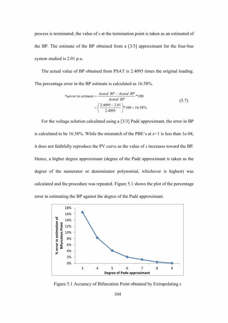
104
process is terminated; the value of s at the termination point is taken as an estimated of
the BP. The estimate of the BP obtained from a [3/3] approximant for the four-bus
system studied is 2.01 p.u.
The actual value of BP obtained from PSAT is 2.4095 times the original loading.
The percentage error in the BP estimate is calculated as 16.58%.
%58.16100*4095.2
01.24095.2
100*%
BPAcutal
BPAcutalBPAcutalestimateinerror
(5.7)
For the voltage solution calculated using a [3/3] Padé approximant, the error in BP
is calculated to be 16.58%. While the mismatch of the PBE’s at s=1 is less than 1e-04,
it does not faithfully reproduce the PV curve as the value of s increases toward the BP.
Hence, a higher degree approximant (degree of the Padé approximant is taken as the
degree of the numerator or denominator polynomial, whichever is highest) was
calculated and the procedure was repeated. Figure 5.1 shows the plot of the percentage
error in estimating the BP against the degree of the Padé approximant.
Figure 5.1 Accuracy of Bifurcation Point obtained by Extrapolating s
0%
2%
4%
6%
8%
10%
12%
14%
16%
18%
3 4 5 6 7 8 9
% e
rro
r in
est
imat
ion
of
B
ifu
rcat
ion
Po
int
Degree of Pade approximant
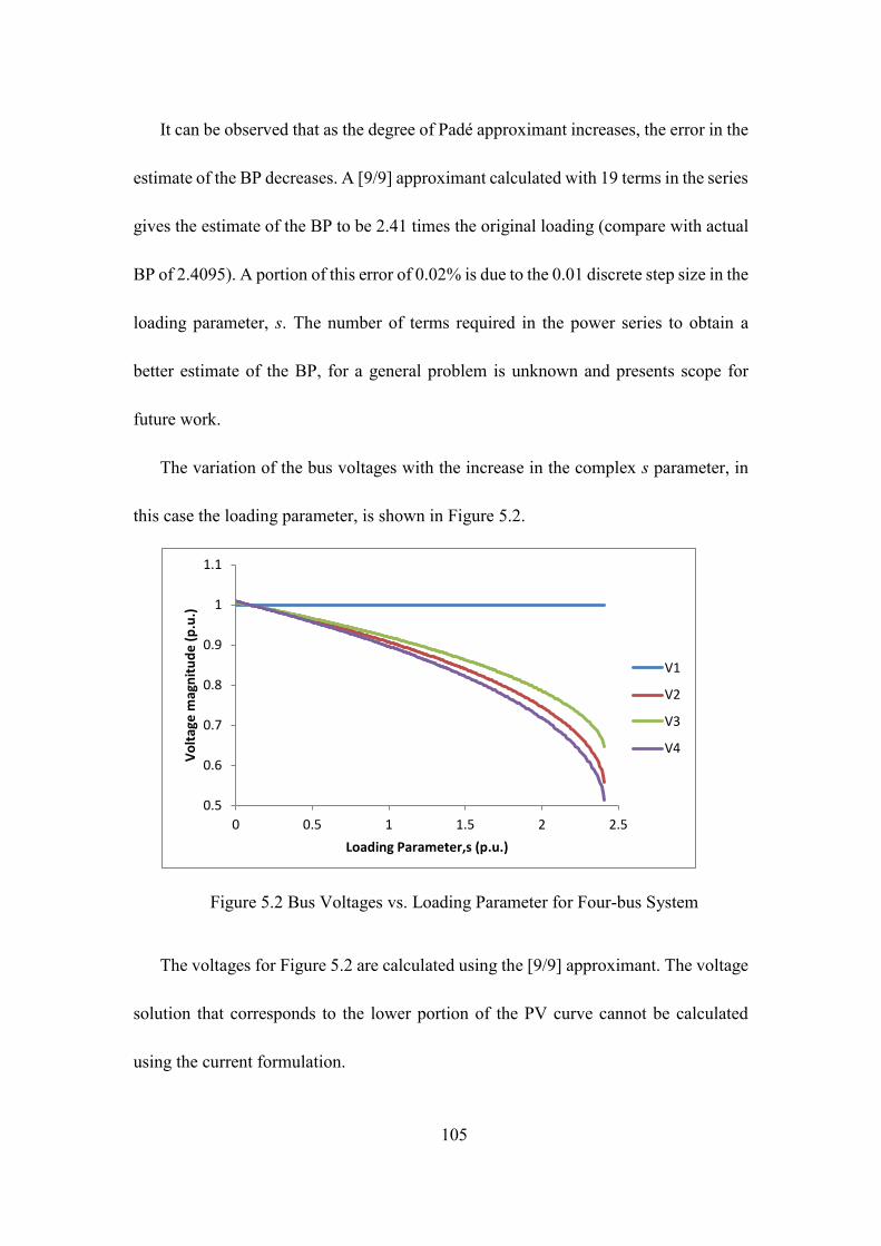
105
It can be observed that as the degree of Padé approximant increases, the error in the
estimate of the BP decreases. A [9/9] approximant calculated with 19 terms in the series
gives the estimate of the BP to be 2.41 times the original loading (compare with actual
BP of 2.4095). A portion of this error of 0.02% is due to the 0.01 discrete step size in the
loading parameter, s. The number of terms required in the power series to obtain a
better estimate of the BP, for a general problem is unknown and presents scope for
future work.
The variation of the bus voltages with the increase in the complex s parameter, in
this case the loading parameter, is shown in Figure 5.2.
Figure 5.2 Bus Voltages vs. Loading Parameter for Four-bus System
The voltages for Figure 5.2 are calculated using the [9/9] approximant. The voltage
solution that corresponds to the lower portion of the PV curve cannot be calculated
using the current formulation.
0.5
0.6
0.7
0.8
0.9
1
1.1
0 0.5 1 1.5 2 2.5
Vo
ltag
e m
agn
itu
de
(p
.u.)
Loading Parameter,s (p.u.)
V1
V2
V3
V4
106
5.4.4 ESTIMATING BIFURCATION POINT USING PADÉ APPROXIMANTS
From the [3/3] Padé approximants of the voltage in Table 5.1, the zeros of the
numerator polynomial of the bus voltages are calculated. For bus 2, the roots of the
numerator polynomial are calculated as:
35.2775.219,0016.08895.5,0013.09095.2
00000.00003.00002.00565.0
0004.05127.00014.00072.132
jjjs
sjsj
sjj
(5.8)
From the previous discussion, it was established that the root of the numerator
polynomial that occurs closest to the origin on or near the real s axis is representative of
the BP. The roots of the numerator polynomial from (5.8) are complex. However, the
value of s by which the loading at each bus has to be scaled before voltage collapse
occurs has to be real. Hence, the estimate of the BP is taken to be the real portion of the
smallest root of the polynomial along the positive s axis i.e. 2.9095 (20.74% error). The
BP estimates can also be obtained from the rational approximants of the other bus
voltages. The error in estimate of the voltage collapse point decreases with an increase
in the number of terms in the series. For instance, the BP estimates for a [10/10] and
[20/20] approximant from V2 are 2.4709 and 2.4308, with error percentages of 2.54%
and 0.88% respectively.
Figure 5.3 and Figure 5.4 show the estimates of the voltage collapse point and the
percentage error in the estimate, respectively, as a function of the degree of the Padé
approximant.

107
Figure 5.3 Estimate of Bifurcation Point Obtained from Padé Approximant
Figure 5.4 Error in Bifurcation Point Obtained from Padé Approximant
5.5 SUMMARY
For a simple four-bus problem with one slack bus and remaining PQ buses, the BP
obtained by uniformly scaling the loads was estimated up to 0.02% accuracy. Tracing
the PV curve was possible by re-evaluating the Padé approximant without resorting to
any CPF technique. Two methods of evaluation of the BP of a system with PQ buses
were presented. The first method involved extrapolating the s parameter; the second
2.4
2.5
2.6
2.7
2.8
2.9
3
3 4 5 6 7 8 9 10 11 12 13 14 15 16 17 18 19 20
Esti
mat
e o
f
Bif
urc
atio
n P
oin
t
Degree of Pade approximant
0%
5%
10%
15%
20%
25%
3 4 5 6 7 8 9 10 11 12 13 14 15 16 17 18 19 20
% e
rro
r in
est
imat
ion
of
B
ifu
rcat
ion
Po
int
Degree of Pade approximant

108
approach calculated the zeros of the numerator polynomial of the Padé approximant. A
comparison of the two methods in calculating the bifurcation point is as follows.
To compare the accuracy of the solution, the BP estimates for the four-bus problem
described above, are obtained from the two methods with the same number of terms in
the series. With 19 terms in the series, the estimate of BP obtained by extrapolating ‘s’
had a percentage error of 0.02%. With the same number of terms in the series, the
estimate of BP from the zeros of the Padé approximant had an error of 3.07%. With 41
terms in the series, the former method of extrapolating ‘s’ yields the same estimate of
BP. The BP estimate and the error percentage remain unaltered due to the step size
chosen (0.01) to increment the s value. With the same 41 terms, using the zeros of the
Padé approximant’s numerator polynomial, the BP estimate found had an error of
0.88%.
In terms of computational complexity, estimating the BP from the zeros of the Padé
approximant requires the calculation of all the roots of a higher degree polynomial. The
method of extrapolating s, on the other hand only requires reevaluating the polynomial
Padé approximant, but multiple times. In the current implementation, this is not quite a
distinguishing feature since calculation of roots of polynomial using software such as
MATLAB is fast.
109
6 CONCLUSION AND FUTURE WORK
6.1 CONCLUSION
The research presented in this document is directed towards implementing a
non-iterative solution procedure for solving the ac power-flow problem, by embedding
the PBE’s as a holomorphic function.
Different techniques for analytic continuation, along with numerical examples were
presented in chapter 3. The numerical issues that should to be taken into consideration
while evaluating the maximal analytic continuation of an analytic function were
demonstrated.
Current literature has an HE model for the load bus. In chapter 4, two different
holomorphically embedded models for the generator bus were developed by:
1. Representing the reactive power injection Qi as a holomorphic function.
2. Eliminating the reactive power term by summing the complex power and its
conjugate.
The details of implementing the HE method to solve the ac PF problem for a small
to medium sized system were presented. The solution procedure was demonstrated in
detail for a sample four-bus system. The HE method was tested on several IEEE test
cases; results from the 118-bus system were presented. The implementation was done
with dense matrix operations in MATLAB. The time taken to solve the 118 bus system
was approximately 0.7 sec. However, the run times and storage requirements would be

110
significantly improved if it were to be programmed in a third generation language (C++,
Java, etc.) with sparsity programming techniques.
A modified HE that allows tracing the PV curve and calculating the bifurcation
point was developed in chapter 5 above. Using the Padé approximants to the voltage
function obtained from HE, it is shown that accurate estimates of the BP can be
obtained, at least for the four-bus problem examined. The solution procedure along
with the theory involved was discussed in detail with numerical examples.
6.2 FUTURE WORK
The HE approach of solving a PF problem should be quantified, compared with the
existing methods on speed of computation, memory requirements and ability to handle
ill-conditioned problems among several other factors. Currently, discontinuities
occurring due to reactive power limits on generators are handled by performing bus
type switching and re-solving the PF problem; a procedure to handle discontinuities
without re-solving the problem could be developed. Numerical testing on a larger scale
model warrants the inclusion of HVDC lines, phase shifting transformers, remote
regulation of buses; in that case, development of a holomorphically embedded model
representative of each component’s original equation becomes necessary. In order to
evaluate the BP using the HE method for a general problem, the generator bus model
ought to be modified and included. Also, a formulation that allows varying the loads
independently at different buses presents scope for future work.
111
REFERENCES
[1] J. D. Glover, M. S. Sarma and T. J. Overbye, “Power System Analysis and Design
4th Edition,” Cengage Learning, Stamford, 2007.
[2] J. B. Ward and H. W. Hale, “Digital Computer Solution of Power-Flow Problems,”
Power Apparatus and Systems, Part III, Transactions of the American Institute of
Electrical Engineers, Jan. 1956, vol. 75, no. 3, pp. 398-404.
[3] W. Tinney and C. Hart, “Power Flow Solution by Newton’s method,” IEEE
Transactions on Power Apparatus and Systems, Nov. 1967, vol. PAS-86, no. 11, pp.
1449-1460.
[4] W. Tinney and J. Walker, “Direct Solution of Sparse Network Equations by
Optimally Ordered Triangular Factorization,” Proceedings of the IEEE, Nov. 1967,
vol. 55, no.11, pp.1801-1809.
[5] B. Stott and O. Alsac, “Fast Decoupled Load Flow,” IEEE Transactions on Power
Apparatus and Systems, May 1974, vol. PAS-93, no. 3, pp. 859-869.
[6] B. Stott, “Decoupled Newton Load Flow,” IEEE Transactions on Power Apparatus
and Systems, Sep. 1972, vol. PAS-91, no. 5, pp. 1955-1959.
[7] S. C. Tripathy, G. D. Prasad, O. P. Malik and G. S. Hope, “Load-Flow Solutions for
Ill-Conditioned Power Systems by a Newton-Like Method,” IEEE Transactions on
Power Apparatus and Systems, Oct. 1982, vol. PAS-101, no.10, pp. 3648-3657.
[8] S. Iwamoto and T. Tamura, “A Load Flow Calculation Method for Ill-Conditioned
Power Systems,” IEEE Transactions on Power Apparatus and Systems, Apr. 1981, vol.
PAS-100, no. 4, pp. 1736-1743.
[9] D. J. Tylavsky, P. E. Crouch, L. F. Jarriel and R. Adapa, “Improved Power Flow
Robustness for Personal Computers,” Industry Applications Society Annual Meeting,
Oct. 1990, vol. 2, no. 7, pp. 1401-1407.
[10] D. J. Tylavsky, P.E. Crouch, L.F. Jarriel, and H. Chen, “Advances in Fast Power
Flow Algorithms,” Advances in Theory and Applications, Control and Dynamics,
Academic Press, 1991, vol. 42, Part 4 of 4, pp. 295-344.
[11] P. Crouch, D. Tylavsky, L. Jarriel and H. Chen, “Critically Coupled Algorithms
for Solving the Power Flow Equation,” IEEE Transactions on Power Systems, Feb.
1992, vol. 7, no. 1, pp. 451-457.

112
[12] D. Tylavsky, P. Crouch, L. Jarriel, J. Singh, and R. Adapa, “The Effects of
Precision and Small Impedance Branches on Power Flow Robustness,” IEEE
Transactions on Power Systems, Feb. 1994, vol. 9, no. 1, pp. 6-14.
[13] M. Schaffer and D. Tylavsky, “A Nondiverging Polar-Form Newton-Based
Power Flow,” IEEE Transactions on Industry Applications, Sep. 1988, vol. 24, no. 5,
pp. 870 -877.
[14] D. Tylavsky and M. Schaffer, “Non-Diverging Power Flow Using a Least-Power
Type Theorem,” IEEE Transactions on Industry Applications, Sep. 1987, vol. IA-23,
no. 5, pp. 944-951.
[15] V. Ajjarapu, “Computational Techniques for Voltage Stability Assessment and
Control,” Springer US, New York, 2006.
[16] C. Taylor, “Power System Voltage Stability,” McGraw Hill, New York, 1994.
[17] U.S.-Canada Power System Outage Task Force, “Final Report on the August 14,
2003 Blackout in the United States and Canada: Causes and Recommendations,” Apr.
2004 available at:
http://energy.gov/sites/prod/files/oeprod/DocumentsandMedia/BlackoutFinalWeb.pdf.
[18] V. Ajjarapu and C. Christy, “The Continuation Power Flow: A Tool for Steady
State Voltage Stability Analysis,” IEEE Transactions on Power Systems, Feb. 1992,
vol. 7, no. 1, pp. 416–423.
[19] C. Canizares and F. L. Alvarado, “Point of Collapse and Continuation Methods for
Large ac/dc Systems,” IEEE Transactions on Power Systems, Feb. 1993, vol. 8, no. 1,
pp. 1–8.
[20] A. Trias, “The Holomorphic Embedding Load Flow Method,” IEEE PES General
Meeting, San Diego, CA, July 2012, pp. 1-8.
[21] A. Trias, “System and Method for Monitoring and Managing Electrical Power
Transmission and Distribution Networks,” US Patents 7,519,506 (2009) and 7,979,239
(2011).
[22] B. Stott, “Review of Load Flow Calculation Methods”, Proceedings of IEEE, July
1974, vo1.62, no. 7, pp. 916-929.
[23] M. Laughton and M. Davies, “Numerical Techniques in the Solution of Power
System Load Flow Problems,” Proceedings of the Institute of Electrical Engineers,
Sept. 1964, vol. 111, no. 9, pp. 1575-1588.
113
[24] G. Huang and W. Ongsakul, “Parallel Implementation of Gauss-Seidel Type
Algorithms for Power Flow Analysis on a SEQUENT Parallel Computer,” Proceedings
of the 20th International Conference of Parallel Processing, 1991, pp. 171 -174.
[25] H. Dommel, W. Tinney and W. Powell, “Further Developments in Newton’s
Method for Power Systems Applications,” IEEE Winter Power Meeting, NewYork,
Jan. 1970.
[26] A. Keyhani, A. Abur and S. Hao, “Evaluation of Power Flow Techniques for
Personal Computers,” IEEE Transactions on Power Systems, May 1989, vol.4, no.2,
pp.817-826.
[27] D. Tylavsky, “Lecture notes on Decoupled Power-flow algorithms,” Computer
Solution of Power Systems, Fall 2012.
[28] P. Sauer, “Explicit Load Flow Series and Functions”, IEEE Transactions on Power
Apparatus and Systems, 1981, vol. PAS-100, no. 8, pp. 3754-3763.
[29] Y. Wang, L. Silva, W. Xu and Y. Zhang, “Analysis of Ill-Conditioned Power-Flow
Problems using Voltage Stability Methodology,” IEEE Proceedings Generation,
Transmission and Distribution, Sep 2001, vol.148, no.5, pp.384-390.
[30] W. Xu, Y. Liu, J. C. Salmon, T. Le and G. Chang, “Series Load Flow: A Novel
Non-Iterative Load Flow Method,” IEEE Proceedings Generation, Transmission and
Distribution, May 1998, vol. 145, no. 3, pp. 251-256.
[31] L. Shao-Hua and Hsiao-Dong Chiang, “Continuation Power Flow with Multiple
Load Variation and Generation Re-Dispatch Patterns,” IEEE Power Engineering
Society General Meeting, 2006.
[32] X. Zhang, P. Ju and E. Handschin, “Continuation Three-Phase Power Flow: A
Tool for Voltage Stability Analysis of Unbalanced Three-Phase Power Systems,” Aug.
2005, IEEE Transactions on Power Systems, vol.20, no.3, pp.1320,1329.
[33] F. L. Alvarado and T. H. Jung, “Direct Detection of Voltage Collapse Conditions,”
Proceedings: Bulk Power System Voltage Phenomena - Voltage Stability and Security,
EPRI EL-6183, Project 2473-21, Electric Power Research Institute, Jan. 1989.
[34] F. L. Alvarado, M. Gu and Y. Hu, “Direct Detection of Instability Points using an
Augmented Formulation,” available at:
http://citeseerx.ist.psu.edu/viewdoc/summary?doi=10.1.1.29.5643
[35] D. Irisarri, X. Wang, J. Tong and S. Mokhtari, “Maximum Loadability of Power
Systems using Interior Point Nonlinear Optimization Method,” IEEE Transactions on
Power Systems, Feb. 1997, vol. 12, no. 1, pp. 162–172.

114
[36] J. Lu, C. W. Liu and J. S. Thorp, “New Methods for Computing a Saddle-Node
Bifurcation Point for Voltage Stability Analysis,” IEEE Transactions on Power
Systems, May 1995, vol. 10, no. 2, pp. 978–985.
[37] C. Vournas, M. Karystianos and N. Maratos, “Bifurcation Points and Loadability
Limits as Solutions of Constrained Optimization Problems,” IEEE Power Engineering
Society Summer Meeting, 2000, vol.3, pp.1883-1888.
[38] A. Yang, “Notes on Functions of a Complex Variable,” available at:
http://www.math.dartmouth.edu/~m43s12/.
[39] Y. Feng, “Solving for the Low-Voltage Power-Flow Solutions by using a
Holomorphic Embedded Formulation,” April 2014, Ph.D. Qualifying exam, School of
Electrical, Computer and Energy Engineering, Arizona State University, pp. 38-41.
[40] R.C.Gunning and H.Rosi, “Analytic Functions of Several Complex Variables,”
American Mathematical Society, 1965, pp.317.
[41] A. Bulthell, “Division Algorithms for Continued Fractions and the Padé Table,”
Journal of Computational and Applied Mathematics, 1980, vol. 6, Issue 4, pp. 259-266.
[42] H. Stahl, “On the Convergence of Generalized Padé Approximants,” Constructive
Approximation, 1989, vol. 5, pp. 221–240.
[43] H. Stahl “The Convergence of Padé Approximants to Functions with Branch
Points,” Journal of Approximation Theory, 1997, vol. 91, no. 2, pp. 139–204.
[44] G. Baker and P. Graves-Morris, “Padé approximants,” Series: Encyclopaedia of
Mathematics and its applications, Cambridge University Press, New York, 1996.
[45] C. G. Small, “Expansions and Asymptotics for Statistics,” Chapman and
Hall/CRC Publications, May 2010, pp. 85-88.
[46] D. Tylavsky, “Lecture Notes on Padé approximants and Nonlinear equations,”
Computer Solution of Power Systems, Spring 2014.
[47] D. Shanks, “Nonlinear Transformations of Divergent and Slowly Convergent
Sequences,” Journal of Mathematical Physics, 1955, vol. 34, pp. 1-42.
[48] P. Wynn, “Upon Systems of Recursion which obtain among Quotients of the Padé
Table,” Journal of Computational and Applied Mathematics, 1966, vol. 5, Issue 4, pp.
264-269.
[49] W.E. Weisstein “Gregory Series,” From MathWorld-A Wolfram Web Resource
available at:
http://mathworld.wolfram.com/GregorySeries.html.

115
[50] E. Cheney and D. Kincaid, “Numerical Mathematics and Computing,” Cengage
Learning, Stamford, August 2007.
[51] M. Subramanian, Y. Feng and D. Tylavsky, “PV Bus Modeling in a
Holomorphically Embedded Power-Flow Formulation,” North American Power
Symposium, Sep. 2013, pp. 1-6.
[52] A. Trias, Personal communication, February 2014.
[53] J.J. Grainger and W.D. Stevenson, “Power Systems Analysis,” McGraw-Hill, New
York, Jan. 1994.
[54] R. Christie, “118 Bus Power Flow Test Case,” May 1993, available at:
http://www.ee.washington.edu/research/pstca/pf118/pg_tca118bus.htm.
[55] M. Subramanian, “Computer Solution of Power Systems-Final project report,”
Arizona State University, Dec. 2012.
[56] F. Milano, “Power Systems Analysis Toolbox,” available at:
http://faraday1.ucd.ie/software.html.

116
APPENDIX A
VOLTAGE SOLUTION FOR IEEE-118 BUS SYSTEM

117
--------------------------------------------------------------------
Converged Bus Voltages
--------------------------------------------------------------------
| Bus |Bus |Type |V |Angle |Generation |
| No |name | |pu |Degree |MW |Mvar |
--------------------------------------------------------------------
1 Riversde 2 0.9550 -19.0177 0.00 -3.10
2 Pokagon 0 0.9714 -18.4777 0.00 0.00
3 HickryCk 0 0.9677 -18.1344 0.00 0.00
4 NwCarlsl 2 0.9980 -14.4169 -9.00 -15.01
5 Olive 0 1.0020 -13.9719 0.00 0.00
6 Kankakee 2 0.9900 -16.6987 0.00 15.93
7 JacksnRd 0 0.9893 -17.1431 0.00 0.00
8 Olive 2 1.0150 -8.9514 -28.00 62.76
9 Bequine 0 1.0429 -1.6973 0.00 0.00
10 Breed 2 1.0500 5.8837 450.00 -51.04
11 SouthBnd 0 0.9851 -16.9845 0.00 0.00
12 TwinBrch 2 0.9900 -17.5012 85.00 91.27
13 Concord 0 0.9683 -18.3594 0.00 0.00
14 GoshenJt 0 0.9836 -18.2174 0.00 0.00
15 FtWayne 2 0.9700 -18.5111 0.00 3.06
16 N.E. 0 0.9839 -17.8028 0.00 0.00
17 Sorenson 0 0.9951 -15.9949 0.00 0.00
18 McKinley 2 0.9730 -18.2086 0.00 25.53
19 Lincoln 4 0.9634 -18.6932 0.00 -8.00
20 Adams 0 0.9581 -17.8133 0.00 0.00
21 Jay 0 0.9586 -16.2254 0.00 0.00
22 Randolph 0 0.9696 -13.6709 0.00 0.00
23 CollCrnr 0 0.9997 -8.7502 0.00 0.00
24 Trenton 2 0.9920 -8.8825 -13.00 -15.28
25 TannrsCk 2 1.0500 -1.8161 220.00 49.80
26 TannrsCk 2 1.0150 -0.0356 314.00 9.90
27 Madison 2 0.9680 -14.3879 -9.00 2.83
28 Mullin 0 0.9616 -16.1125 0.00 0.00
29 Grant 0 0.9632 -17.1049 0.00 0.00
30 Sorenson 0 0.9855 -10.9604 0.00 0.00
31 DeerCrk 2 0.9670 -16.9880 7.00 31.98
32 Delaware 4 0.9636 -14.9405 0.00 -14.00
33 Haviland 0 0.9716 -19.1361 0.00 0.00
34 Rockhill 4 0.9859 -18.4941 0.00 -8.00
35 WestLima 0 0.9807 -18.9213 0.00 0.00
36 Sterling 2 0.9800 -18.9168 0.00 -1.25
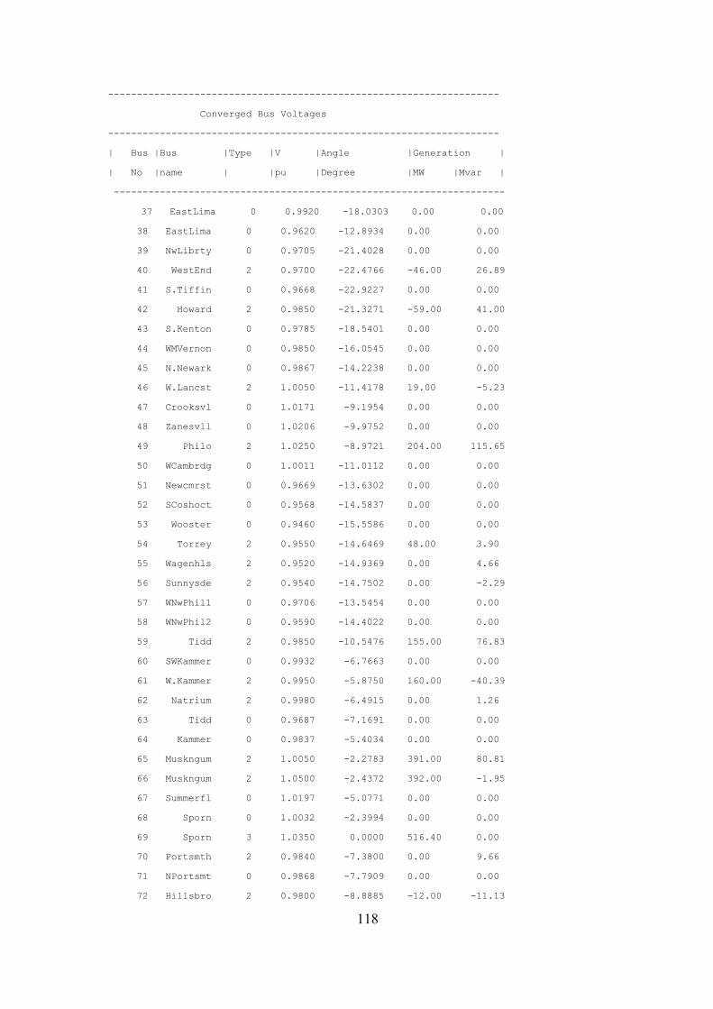
118
--------------------------------------------------------------------
Converged Bus Voltages
--------------------------------------------------------------------
| Bus |Bus |Type |V |Angle |Generation |
| No |name | |pu |Degree |MW |Mvar |
--------------------------------------------------------------------
37 EastLima 0 0.9920 -18.0303 0.00 0.00
38 EastLima 0 0.9620 -12.8934 0.00 0.00
39 NwLibrty 0 0.9705 -21.4028 0.00 0.00
40 WestEnd 2 0.9700 -22.4766 -46.00 26.89
41 S.Tiffin 0 0.9668 -22.9227 0.00 0.00
42 Howard 2 0.9850 -21.3271 -59.00 41.00
43 S.Kenton 0 0.9785 -18.5401 0.00 0.00
44 WMVernon 0 0.9850 -16.0545 0.00 0.00
45 N.Newark 0 0.9867 -14.2238 0.00 0.00
46 W.Lancst 2 1.0050 -11.4178 19.00 -5.23
47 Crooksvl 0 1.0171 -9.1954 0.00 0.00
48 Zanesvll 0 1.0206 -9.9752 0.00 0.00
49 Philo 2 1.0250 -8.9721 204.00 115.65
50 WCambrdg 0 1.0011 -11.0112 0.00 0.00
51 Newcmrst 0 0.9669 -13.6302 0.00 0.00
52 SCoshoct 0 0.9568 -14.5837 0.00 0.00
53 Wooster 0 0.9460 -15.5586 0.00 0.00
54 Torrey 2 0.9550 -14.6469 48.00 3.90
55 Wagenhls 2 0.9520 -14.9369 0.00 4.66
56 Sunnysde 2 0.9540 -14.7502 0.00 -2.29
57 WNwPhil1 0 0.9706 -13.5454 0.00 0.00
58 WNwPhil2 0 0.9590 -14.4022 0.00 0.00
59 Tidd 2 0.9850 -10.5476 155.00 76.83
60 SWKammer 0 0.9932 -6.7663 0.00 0.00
61 W.Kammer 2 0.9950 -5.8750 160.00 -40.39
62 Natrium 2 0.9980 -6.4915 0.00 1.26
63 Tidd 0 0.9687 -7.1691 0.00 0.00
64 Kammer 0 0.9837 -5.4034 0.00 0.00
65 Muskngum 2 1.0050 -2.2783 391.00 80.81
66 Muskngum 2 1.0500 -2.4372 392.00 -1.95
67 Summerfl 0 1.0197 -5.0771 0.00 0.00
68 Sporn 0 1.0032 -2.3994 0.00 0.00
69 Sporn 3 1.0350 0.0000 516.40 0.00
70 Portsmth 2 0.9840 -7.3800 0.00 9.66
71 NPortsmt 0 0.9868 -7.7909 0.00 0.00
72 Hillsbro 2 0.9800 -8.8885 -12.00 -11.13

119
--------------------------------------------------------------------
Converged Bus Voltages
--------------------------------------------------------------------
| Bus |Bus |Type |V |Angle |Generation |
| No |name | |pu |Degree |MW |Mvar |
--------------------------------------------------------------------
73 Sargents 2 0.9910 -8.0024 -6.00 9.65
74 Bellefnt 2 0.9580 -8.3288 0.00 -5.63
75 SthPoint 0 0.9673 -7.0670 0.00 0.00
76 Darrah 2 0.9430 -8.1970 0.00 5.27
77 Turner 2 1.0060 -3.2431 0.00 11.94
78 Chemical 0 1.0034 -3.5470 0.00 0.00
79 CapitlHl 0 1.0092 -3.2478 0.00 0.00
80 CabinCrk 2 1.0400 -1.0023 477.00 105.04
81 Kanawha 0 0.9968 -1.8505 0.00 0.00
82 Logan 0 0.9887 -2.7227 0.00 0.00
83 Sprigg 0 0.9845 -1.5326 0.00 0.00
84 BetsyLne 0 0.9798 1.0008 0.00 0.00
85 BeaverCk 2 0.9850 2.5549 0.00 -5.77
86 Hazard 0 0.9867 1.1854 0.00 0.00
87 Pinevlle 2 1.0150 1.4447 4.00 11.02
88 Fremont 0 0.9875 5.6859 0.00 0.00
89 ClinchRv 2 1.0050 9.7414 607.00 -11.79
90 Holston 2 0.9850 3.3365 -85.00 59.30
91 HolstonT 2 0.9800 3.3555 -10.00 -14.85
92 Saltvlle 4 0.9923 3.8545 0.00 -3.00
93 Tazewell 0 0.9869 0.8434 0.00 0.00
94 Switchbk 0 0.9906 -1.3105 0.00 0.00
95 Caldwell 0 0.9809 -2.2823 0.00 0.00
96 Baileysv 0 0.9927 -2.4496 0.00 0.00
97 Sundial 0 1.0114 -2.0764 0.00 0.00
98 Bradley 0 1.0235 -2.5539 0.00 0.00
99 Hinton 2 1.0100 -2.9157 -42.00 -17.54
100 GlenLyn 2 1.0170 -1.9196 252.00 110.08
101 Wythe 0 0.9924 -0.3468 0.00 0.00
102 Smythe 0 0.9910 2.3511 0.00 0.00
103 Claytor 5 1.0007 -5.5146 40.00 40.00
104 Hancock 2 0.9710 -8.2595 0.00 5.65
105 Roanoke 4 0.9660 -9.3816 0.00 -8.00
106 Cloverdl 0 0.9618 -9.6295 0.00 0.00
107 Reusens 2 0.9520 -12.4196 -22.00 5.70
108 Blaine 0 0.9668 -10.5725 0.00 0.00

120
--------------------------------------------------------------------
Converged Bus Voltages
--------------------------------------------------------------------
| Bus |Bus |Type |V |Angle |Generation |
| No |name | |pu |Degree |MW |Mvar |
--------------------------------------------------------------------
109 Franklin 0 0.9675 -11.0218 0.00 0.00
110 Fieldale 2 0.9730 -11.8606 0.00 4.86
111 DanRiver 2 0.9800 -10.2155 36.00 -1.84
112 Danville 2 0.9750 -14.9598 -43.00 41.51
113 DeerCrk 2 0.9930 -15.9969 -6.00 6.32
114 WMedford 0 0.9604 -15.2708 0.00 0.00
115 Medford 0 0.9603 -15.2784 0.00 0.00
116 KygerCrk 2 1.0050 -2.8344 -184.00 51.32
117 Corey 0 0.9738 -19.0422 0.00 0.00
118 WHuntngd 0 0.9494 -8.0547 0.00 0.00

121
--------------------------------------------------------------------
Line flows in branches and Tap ratios
--------------------------------------------------------------------
Branch |Tap |Z |Tap |From bus injection|To bus injection |
|Bus |Bus |Ratio |P(M.W.) |Q(MVar)|P(M.W.) |Q(MVar)|
--------------------------------------------------------------------
1 1 2 0.000 -12.36 -13.04 12.45 11.01
2 1 3 0.000 -38.64 -17.06 38.89 16.89
3 4 5 0.000 -103.21 -26.79 103.41 27.49
4 3 5 0.000 -68.10 -14.49 69.34 17.28
5 5 6 0.000 88.46 4.11 -87.53 -1.30
6 6 7 0.000 35.53 -4.77 -35.47 4.50
7 8 9 0.000 -440.64 -89.73 445.25 24.43
8 8 5 0.985 338.42 124.72 -338.42 -92.01
9 9 10 0.000 -445.25 -24.43 450.00 -51.04
10 4 11 0.000 64.21 -0.21 -63.35 1.34
11 5 11 0.000 77.21 2.97 -76.00 -0.63
12 11 12 0.000 34.28 -35.13 -34.14 35.13
13 2 12 0.000 -32.45 -20.01 32.74 19.42
14 3 12 0.000 -9.79 -12.39 9.90 8.86
15 7 12 0.000 16.47 -6.50 -16.44 5.75
16 11 13 0.000 35.06 11.41 -34.74 -12.16
17 12 14 0.000 18.29 2.63 -18.21 -4.15
18 13 15 0.000 0.74 -3.84 -0.74 -2.05
19 14 15 0.000 4.21 3.15 -4.18 -7.84
20 12 16 0.000 7.50 4.29 -7.49 -6.30
21 15 17 0.000 -103.72 -24.41 105.30 25.36
22 16 17 0.000 -17.51 -3.70 17.66 -0.29
23 17 18 0.000 80.27 24.85 -79.39 -22.49
24 18 19 0.000 19.39 14.02 -19.32 -14.79
25 19 20 0.000 -10.65 5.42 10.69 -7.97
26 15 19 0.000 11.41 12.25 -11.37 -13.07
27 20 21 0.000 -28.69 4.97 28.86 -6.16
28 21 22 0.000 -42.86 -1.84 43.28 1.49
29 22 23 0.000 -53.28 -6.49 54.32 7.41
30 23 24 0.000 8.30 10.80 -8.26 -15.61
31 23 25 0.000 -162.61 -25.92 166.81 38.38
32 26 25 0.960 90.30 21.58 -90.30 -18.64
33 25 27 0.000 143.49 30.06 -137.09 -15.27
34 27 28 0.000 32.86 -0.59 -32.64 -0.44
35 28 29 0.000 15.64 -6.56 -15.57 4.64
36 30 17 0.960 231.06 93.37 -231.06 -70.51

122
--------------------------------------------------------------------
Line flows in branches and Tap ratios
--------------------------------------------------------------------
Branch |Tap |Z |Tap |From bus injection|To bus injection |
|Bus |Bus |Ratio |P(M.W.) |Q(MVar)|P(M.W.) |Q(MVar)|
--------------------------------------------------------------------
37 8 30 0.000 74.22 27.77 -73.87 -75.07
38 26 30 0.000 223.70 -11.68 -219.72 -36.38
39 17 31 0.000 14.77 11.55 -14.58 -14.76
40 29 31 0.000 -8.43 -8.64 8.45 7.92
41 23 32 0.000 92.99 4.71 -90.21 -5.91
42 31 32 0.000 -29.87 11.82 30.21 -13.04
43 27 32 0.000 12.50 1.02 -12.46 -2.69
44 15 33 0.000 7.23 -4.88 -7.20 1.96
45 19 34 0.000 -3.66 -10.57 3.72 4.75
46 35 36 0.000 0.67 6.25 -0.67 -6.50
47 35 37 0.000 -33.67 -15.25 33.82 14.66
48 33 37 0.000 -15.80 -10.96 15.94 7.93
49 34 36 0.000 30.43 11.50 -30.33 -11.75
50 34 37 0.000 -94.58 -38.57 94.86 38.61
51 38 37 0.935 243.68 112.11 -243.68 -86.62
52 37 39 0.000 54.96 3.75 -53.97 -3.07
53 37 40 0.000 44.10 -2.93 -42.93 2.21
54 30 38 0.000 62.53 18.08 -62.28 -55.10
55 39 40 0.000 26.97 -7.93 -26.82 6.97
56 40 41 0.000 15.51 1.17 -15.48 -2.19
57 40 42 0.000 -11.77 -6.47 11.86 2.32
58 41 42 0.000 -21.52 -7.81 21.74 5.26
59 43 44 0.000 -16.57 -1.03 16.75 -4.10
60 34 43 0.000 1.44 1.92 -1.43 -5.97
61 44 45 0.000 -32.75 5.81 33.00 -6.94
62 45 46 0.000 -36.32 -3.38 36.86 1.92
63 46 47 0.000 -31.10 -1.22 31.46 -0.79
64 46 48 0.000 -14.76 -5.83 14.90 1.42
65 47 49 0.000 -9.55 -10.83 9.59 9.27
66 42 49 0.000 -64.80 5.21 67.96 0.37
67 42 49 0.000 -64.80 5.21 67.96 0.37
68 45 49 0.000 -49.69 -1.95 51.42 2.17
69 48 49 0.000 -34.90 3.21 35.11 -3.92
70 49 50 0.000 53.67 13.43 -52.88 -13.14
71 49 51 0.000 66.64 20.44 -64.35 -17.40
72 51 52 0.000 28.56 6.24 -28.37 -6.99

123
--------------------------------------------------------------------
Line flows in branches and Tap ratios
--------------------------------------------------------------------
Branch |Tap |Z |Tap |From bus injection|To bus injection |
|Bus |Bus |Ratio |P(M.W.) |Q(MVar)|P(M.W.) |Q(MVar)|
--------------------------------------------------------------------
73 52 53 0.000 10.37 1.99 -10.32 -5.45
74 53 54 0.000 -12.68 -5.55 12.73 2.99
75 49 54 0.000 37.77 13.07 -36.58 -15.60
76 49 54 0.000 37.75 11.20 -36.39 -13.79
77 54 55 0.000 7.08 1.46 -7.07 -3.25
78 54 56 0.000 18.53 4.34 -18.52 -4.97
79 55 56 0.000 -21.43 -5.82 21.45 5.56
80 56 57 0.000 -22.99 -9.10 23.22 7.49
81 50 57 0.000 35.88 9.14 -35.22 -10.49
82 56 58 0.000 -6.67 -3.69 6.69 1.53
83 51 58 0.000 18.79 3.16 -18.69 -4.53
84 54 59 0.000 -30.38 -7.51 30.90 4.26
85 56 59 0.000 -27.96 -4.18 28.67 0.99
86 56 59 0.000 -29.31 -3.91 30.07 1.13
87 55 59 0.000 -34.51 -8.26 35.15 5.88
88 59 60 0.000 -43.31 3.57 43.94 -4.40
89 59 61 0.000 -51.71 5.03 52.63 -4.63
90 60 61 0.000 -112.06 8.52 112.40 -8.23
91 60 62 0.000 -9.87 -7.11 9.89 5.74
92 61 62 0.000 25.49 -13.86 -25.42 13.20
93 63 59 0.960 151.75 67.48 -151.75 -57.03
94 63 64 0.000 -151.75 -67.48 152.23 52.51
95 64 61 0.985 30.52 13.99 -30.52 -13.69
96 38 65 0.000 -181.41 -57.01 184.62 -9.07
97 64 65 0.000 -182.76 -66.49 183.75 40.06
98 49 66 0.000 -132.18 4.31 135.18 8.33
99 49 66 0.000 -132.18 4.31 135.18 8.33
100 62 66 0.000 -37.17 -17.26 37.93 14.68
101 62 67 0.000 -24.31 -14.41 24.50 12.15
102 65 66 0.935 8.46 72.25 -8.46 -70.55
103 66 67 0.000 53.16 19.27 -52.50 -19.15
104 65 68 0.000 14.17 -22.43 -14.16 -41.85
105 47 69 0.000 -55.91 11.62 58.65 -10.06
106 49 69 0.000 -46.51 10.63 48.75 -12.05
107 68 69 0.935 -125.66 112.81 125.66 -103.65
108 69 70 0.000 108.35 16.08 -104.92 -13.99

124
--------------------------------------------------------------------
Line flows in branches and Tap ratios
--------------------------------------------------------------------
Branch |Tap |Z |Tap |From bus injection|To bus injection |
|Bus |Bus |Ratio |P(M.W.) |Q(MVar)|P(M.W.) |Q(MVar)|
--------------------------------------------------------------------
109 24 70 0.000 -6.21 -2.97 6.21 -6.80
110 70 71 0.000 16.65 -12.38 -16.61 11.68
111 24 72 0.000 1.47 3.31 -1.46 -7.98
112 71 72 0.000 10.60 -0.94 -10.54 -3.15
113 71 73 0.000 6.01 -10.74 -6.00 9.65
114 70 74 0.000 16.20 12.89 -16.01 -15.42
115 70 75 0.000 -0.14 9.94 0.20 -13.17
116 69 75 0.000 109.97 20.49 -105.12 -18.32
117 74 75 0.000 -51.99 -6.19 52.36 6.44
118 76 77 0.000 -61.17 -21.03 63.23 24.39
119 69 77 0.000 62.10 6.81 -60.95 -13.84
120 75 77 0.000 -34.63 -9.54 35.44 7.37
121 77 78 0.000 45.37 6.62 -45.29 -7.63
122 78 79 0.000 -25.71 -18.37 25.76 17.95
123 77 80 0.000 -96.62 -37.40 98.39 37.52
124 77 80 0.000 -44.39 -20.54 45.07 20.59
125 79 80 0.000 -64.76 -29.58 65.53 31.08
126 68 81 0.000 -44.30 -4.61 44.36 -75.55
127 81 80 0.935 -44.36 75.55 44.36 -73.05
128 77 82 0.000 -3.09 17.34 3.23 -25.08
129 82 83 0.000 -47.11 24.51 47.44 -27.11
130 83 84 0.000 -24.73 14.73 25.29 -16.04
131 83 85 0.000 -42.71 12.07 43.60 -12.37
132 84 85 0.000 -36.29 9.04 36.74 -9.29
133 85 86 0.000 17.17 -7.35 -17.05 5.09
134 86 87 0.000 -3.95 -15.09 4.00 11.02
135 85 88 0.000 -50.33 7.58 50.87 -7.52
136 85 89 0.000 -71.18 0.66 72.43 3.73
137 88 89 0.000 -98.87 -2.48 100.27 7.70
138 89 90 0.000 58.17 -4.72 -56.44 5.80
139 89 90 0.000 110.74 -5.43 -107.85 7.04
140 90 91 0.000 1.29 4.46 -1.28 -6.50
141 89 92 0.000 201.79 -6.59 -197.80 21.49
142 89 92 0.000 63.60 -6.49 -62.02 8.72
143 91 92 0.000 -8.72 -8.35 8.77 5.33
144 92 93 0.000 57.71 -10.75 -56.82 11.57

125
145 92 94 0.000 52.26 -14.31 -50.85 14.95
146 93 94 0.000 44.82 -18.57 -44.29 18.48
147 94 95 0.000 40.98 9.34 -40.74 -9.63
148 80 96 0.000 18.93 20.85 -18.63 -24.42
149 82 96 0.000 -10.12 -6.87 10.14 1.60
150 94 96 0.000 19.91 -9.46 -19.79 7.61
151 80 97 0.000 26.38 25.54 -26.14 -26.98
152 80 98 0.000 28.86 8.33 -28.66 -10.45
153 80 99 0.000 19.48 8.18 -19.27 -12.96
154 92 100 0.000 31.45 -15.81 -30.68 14.56
155 94 100 0.000 4.24 -49.30 -3.85 44.49
156 95 96 0.000 -1.26 -21.37 1.34 20.18
157 96 97 0.000 -11.06 -19.97 11.14 17.98
158 98 100 0.000 -5.34 2.45 5.36 -7.31
159 99 100 0.000 -22.73 -4.57 22.83 2.78
160 100 101 0.000 -16.73 22.07 16.96 -24.35
161 92 102 0.000 44.62 -7.67 -44.37 7.39
162 101 102 0.000 -38.96 9.35 39.37 -10.39
163 100 103 0.000 121.08 -4.30 -118.82 6.29
164 100 104 0.000 56.42 10.62 -54.95 -9.34
165 103 104 0.000 32.31 7.93 -31.78 -10.08
166 103 105 0.000 42.95 6.55 -41.92 -7.39
167 100 106 0.000 60.57 9.17 -58.34 -6.78
168 104 105 0.000 48.73 0.07 -48.48 -0.04
169 105 106 0.000 8.68 4.55 -8.67 -5.82
170 105 107 0.000 26.73 -1.85 -26.33 -1.09
171 105 108 0.000 23.99 -10.61 -23.80 9.39
172 106 107 0.000 24.00 -3.40 -23.67 0.22
173 108 109 0.000 21.80 -10.39 -21.74 9.86
174 103 110 0.000 60.56 3.23 -59.11 -1.03
175 109 110 0.000 13.74 -12.86 -13.64 11.23
176 110 111 0.000 -35.70 0.96 36.00 -1.84
177 110 112 0.000 69.46 -30.61 -68.00 28.51
178 17 113 0.000 2.06 6.04 -2.06 -6.79
179 32 113 0.000 4.11 -17.53 -3.94 13.11
180 32 114 0.000 9.36 2.17 -9.35 -3.61
181 27 115 0.000 20.73 4.67 -20.65 -6.13
182 114 115 0.000 1.35 0.61 -1.35 -0.87
183 68 116 0.000 184.13 -66.36 -184.00 51.32
184 12 117 0.000 20.15 5.20 -20.00 -8.00
185 75 118 0.000 40.19 23.59 -39.85 -23.56
186 76 118 0.000 -6.83 -9.70 6.85 8.56