Application of Improved Feature Selection Algorithm in SVM

Portland State University Portland State University

PDXScholar PDXScholar

Dissertations and Theses Dissertations and Theses

Fall 1-18-2019

Application of Improved Feature Selection Algorithm Application of Improved Feature Selection Algorithm

in SVM Based Market Trend Prediction Model in SVM Based Market Trend Prediction Model

Qi Li Portland State University

Follow this and additional works at: https://pdxscholar.library.pdx.edu/open_access_etds

Part of the Electrical and Computer Engineering Commons

Let us know how access to this document benefits you.

Recommended Citation Recommended Citation Li, Qi, "Application of Improved Feature Selection Algorithm in SVM Based Market Trend Prediction Model" (2019). Dissertations and Theses. Paper 4730. https://doi.org/10.15760/etd.6614

This Thesis is brought to you for free and open access. It has been accepted for inclusion in Dissertations and Theses by an authorized administrator of PDXScholar. Please contact us if we can make this document more accessible: [email protected].

https://pdxscholar.library.pdx.edu/

https://pdxscholar.library.pdx.edu/open_access_etds

https://pdxscholar.library.pdx.edu/etds

https://pdxscholar.library.pdx.edu/open_access_etds?utm_source=pdxscholar.library.pdx.edu%2Fopen_access_etds%2F4730&utm_medium=PDF&utm_campaign=PDFCoverPages

http://network.bepress.com/hgg/discipline/266?utm_source=pdxscholar.library.pdx.edu%2Fopen_access_etds%2F4730&utm_medium=PDF&utm_campaign=PDFCoverPages

http://library.pdx.edu/services/pdxscholar-services/pdxscholar-feedback/

https://doi.org/10.15760/etd.6614

mailto:[email protected]

Application of Improved Feature Selection Algorithm in

SVM Based Market Trend Prediction Model

by

Qi Li

A thesis submitted in partial fulfillment of the requirements for the degree of

Master of Science in

Electrical and Computer Engineering

Thesis Committee: Fu Li, Chair

James Morris Xiaoyu Song

Portland State University 2018

© 2018 Qi Li

i

Abstract

In this study, a Prediction Accuracy Based Hill Climbing Feature Selection Algorithm

(AHCFS) is created and compared with an Error Rate Based Sequential Feature

Selection Algorithm (ERFS) which is an existing Matlab algorithm. The goal of the study

is to create a new piece of an algorithm that has potential to outperform the existing

Matlab sequential feature selection algorithm in predicting the movement of S&P 500

(^GSPC) prices under certain circumstances. The two algorithms are tested based on

historical data of ^GSPC, and Support Vector Machine (SVM) is employed by both as the

classifier. A prediction without feature selection algorithm implemented is carried out

and used as a baseline for comparison between the two algorithms. The prediction

horizon set in this study for both algorithms varies from one to 60 days. The study

results show that AHCFS reaches higher prediction accuracy than ERFS in the majority of

the cases.

ii

Table of Contents

Abstract………………………………………………………………………………………………………………………………………i

Table of Contents ...........................................................................................................................ii

List of Tables…………………………………………………………………………………………………………………………….iv

List of Figures……………………………………………………………………………………………………………………………. v

Chapter 1 Introduction ................................................................................................................. 1

1.1 Technical Analysis ................................................................................................................. 1

1.2 Theoretical Insights .............................................................................................................2

1.2.1 The Dow Theory ........................................................................................................... 2

1.2.2 Efficient Market Hypothesis .......................................................................................4

1.2.3 Random Walk Theory ..................................................................................................4

1.2.4 Behavioral Finance .......................................................................................................4

1.3 Combination of Technical Analysis and Artificial Intelligence ......................................5

1.4 Problem Statement .............................................................................................................5

1.5 Thesis Structure .................................................................................................................. 6

Chapter 2 Background Information and Literature Review .................................................... 7

2.1 Support Vector Machine (SVM) ........................................................................................7

2.2 Technical Indicators (TIs) .................................................................................................10

2.3 Hypothesis ......................................................................................................................22

2.4 Goal ................................................................................................................................ 23

2.5 Evaluation Method ........................................................................................................23

Chapter 3 Experiment Design ....................................................................................................24

3.1 Data Construction .............................................................................................................24

3.2 Classification ......................................................................................................................25

3.3 Data Pre-processing .......................................................................................................... 25

3.3.1 Interpolation ...............................................................................................................25

3.3.2 Normalization............................................................................................................. 26

iii

3.4 Feature Selection ..............................................................................................................27

3.4.1 General ........................................................................................................................27

3.4.2 Control Group – Strategy #0 .................................................................................... 28

3.4.3 Experiment #1 – Strategy #1 ....................................................................................29

3.4.4 Experiment #2 – Strategy #2 ....................................................................................33

Chapter 4 Results and Discussion .............................................................................................38

4.1 Effectiveness and stability of SVM based feature selection algorithm .....................38

4.2 Scenario 1: Experiment based on the most recent data (2007–2017) ......................39

4.3 Scenario 2: Experiment based on data with sharp changes (2000–2010) ................ 45

4.4 Scenario 3: Experiment based on older data (1992–2002) ........................................ 50

4.5 Scenario 4: Experiment based on much older data (1960-1970) ...............................55

4.6 Others .................................................................................................................................60

Chapter 5 Conclusion and Future Work ....................................................................................61

References……………………………………………………………………………………………………………………………….63

Appendix A Summary Data Sheets .......................................................................................68

2007-2017 .................................................................................................................................68

2000-2010 .................................................................................................................................70

1992-2002 .................................................................................................................................72

1960-1970 .................................................................................................................................74

Appendix B Maltab Codes ......................................................................................................76

SVM based prediction with AHCFS as a feature selection method ..................................76

SVM based prediction with ERFS as a feature selection method .....................................81

SVM based prediction without feature selection ...............................................................86

Sub Functions ...........................................................................................................................90

Appendix C Supplemental Files .......................................................................................... 108

iv

List of Tables

Table 4. 1 Testing (OOS) accuracies for 2007-2017 ...............................................................42

Table 4. 2 Improvement by ERFS vs. by AHCFS (baseline: no feature selection) ..............43







v

List of Figures

Figure 3. 1 Flowchart of SVM classification model without feature selection (Strategy #0) ........ 27

Figure 3. 2 Flowchart of SVM classification model with feature selection (Strategy #1 &

Strategy #2) .................................................................................................................................. 29

Figure 3. 3 Flowchart of feature selection (Part 1) .................................................................30

Figure 3. 4 Flowchart of feature selection (Part 2) .................................................................38

Figure 4. 1 2007-2017 S&P500 ^GSPC trending .....................................................................40




1

Chapter 1 Introduction

Financial markets are becoming more and more significant in the modern economic

system [1]. Nowadays, the stock market is an essential component of the global

economy. Each stock market plays a pivotal role in many fields, and the state of a

nation's stock market somewhat represents its economic status. Due to the

fundamental importance of stock markets, significant effort has been put into studies

regarding market behaviors. One of the many major topics is predicting stock price.

1.1 Technical Analysis

Technical analysis seems to have first appeared in 18th century Japan [2]. The first

version, the Japanese version, of technical analysis was based on candle charts. It is

currently one of the most popular tools and was first created and used by a wealthy

merchant.

In recent years, computing power is becoming more powerful and cheaper. Thus it is

more accessible. Meanwhile, artificial intelligence develops rapidly, such as machine

learning. Many efforts have been put into the study of predicting stock prices and many

theories have come into being [3]. Besides the traditional analysis method, fundamental

analysis (FA), a new method, technical analysis (TA) is actively used in stock price

forecasting [4]. The FA evaluates the intrinsic value of a company’s stock price by

delving into the company’s financial statements [5]. The FA evaluation is a quantitative

analysis based on the company’s revenues, expenses, assets, liabilities, and all the other

financial aspects. The analysis will yield a lot of measurements of the company’s

2

financial status as well as a comprehensive projection based on experience-adjusted risk

parameters. These will then be used to determine the intrinsic value of a company’s

stock price. On the other hand, the TA, as a nontraditional method, is quite the

opposite. The TA method uses a company’s historical data regarding stock price, other

related prices, and other non-price information to identify and summarize existing

patterns and to suggest future movements instead of measuring intrinsic value.

More straightforward, the FA method predicts stock price by finding out and explaining

what the underlying assets of the stock are and how the stock works; the TA method

predicts the stock price by only tracking and learning the stock price and related

information to find a pattern for future use. In sum, FA seeks to understand and explain

the entire system to provide a prediction while TA lets the data take priority and speak

for itself.

1.2 Theoretical Insights

1.2.1 The Dow Theory

Charles Dow, the father of modern TA in the West, provides the initial basis for the

further development of TA, which is now called the Dow Theory [6], [7]. Summarized by

his followers, the Dow Theory includes six tenets/principles.

1. The Averages Discount Everything. Every single factor, which is likely to have an

influence on both demand and supply, is reflected in the market price.

3

2. The Market Has Three Trends. A primary trend lasts for more than a year; a

secondary trend lasts from 3 weeks to 3 months; minor trends last less than

three weeks.

3. Major Trends Have Three Phases

In the first stage, Accumulation Phase, investors enter; in the second stage, the

Public Participation Phase, prices rapidly rise, and economic news becomes

favorable; in the third state, the Distribution Phase, economic conditions peak,

and public participation increases.

4. The Averages Must Confirm Each Other

The Industrial Average and Rail Average (now it is the Dow Jones Transportation

Average) must confirm each other.

5. Volume Must Confirm the Trend

The Dow recognizes volume as a secondary indicator, ranked second only to

price. Volume should expand in the direction of the primary/major (price) trend.

6. A Trend Is Assumed to Be Continuous until Definite Signal of Its Reversal

Trends exist.

It occurs regardless of "market noise." Prices continue going in the same

direction despite the short period of opposite movement. It lasts for a while until

a reversal signal occurs.

Based on these six principles, TA is generally understood as based on the following three

principles:

4

• Price Discounts Everything

• Prices Move in Trends

• History Repeats Itself

1.2.2 Efficient Market Hypothesis

The Efficient Market Hypothesis (EMH) states that: “at any given time, security prices

fully reflect all available information” [8]. EMH indicates that TA will not be useful. If the

current price fully reflects all the information and states that previous prices cannot be

used to predict future prices, EMH implies that no investment strategy can outperform

the market.

1.2.3 Random Walk Theory

This theory states that stock market prices evolve according to a random walk and thus

cannot be predicted [9]. It is consistent with EMH and contradicts the application of TA.

1.2.4 Behavioral Finance

EMH and random walk theories both ignore market realities by assuming that all

participants are entirely rational. Behavioral finance studies investor's market behavior

that derives from the psychological principles of decision making to explain why people

buy and/or sell stocks [10]. A few of the behavioral biases discussed in this chapter

might contribute to such trends and patterns. Further, TA based on historical data is

able to discover trends and patterns to predict the future.

5

With the support of behavioral finance, a new theory – Adaptive Market Hypothesis

(AMH) – started to reconcile economic theories based on EMH with behavioral finance

[11].

1.3 Combination of Technical Analysis and Artificial Intelligence

With the development of computational power in recent years, it is found that the

application of artificial intelligence in TA can be very powerful and has excellent

potential to bring changes on how to predict the market. A multitude of machine

learning techniques is applied to TA to attempt to improve market prediction accuracy

[12], [13], [14].

Simply put, TA uses technical indicators which are derived from stock prices, including

open, close, high, and low prices, and volume as input to attempt to determine future

trends and decide when to buy or sell stocks. Beyond this, there are many studies

combining TA and artificial intelligence (AI), from which a much better prediction model

could be achieved. For example, an Artificial Neural Network (ANN) is used for stock

prediction [15], [16]. At present, Support Vector Machines (SVM), which works similarly

to ANN, is used extensively in this field [17], [18].

1.4 Problem Statement

SVM works as a prediction model with a multitude of adjustable parameters. Technical

indicators (TIs) are used as input features to fine-tune those parameters [19]. Then, the

trained SVM based prediction model is used to predict future movement in stock prices.

That leads to another question: how many and what kinds of indicators/information are

6

best for SVM training? Common sense would suggest that the more information, the

better. However, further studies indicate that increasing the number of SVM features

will reduce performance. One important reason for this is the overfitting problem. This

is the problem of feature selection [20].

Many algorithms have been developed to solve the problem of choosing the best

features for SVM [21], among which the sequential feature selection function (a Matlab

function “sequentialfs”) is a good one [22]. This function is an error rate, filter-based,

sequential feature selection algorithm (we call it ERFS in later discussion). Besides this

function, another improved sequential feature selection method is developed and

tested in this study, which promotes prediction accuracy. The improved method is a

prediction accuracy based hill climbing feature selection algorithm or AHCFS.

1.5 Thesis Structure

Chapter 1 introduced the development of market prediction, stated the problem that

will be covered in this thesis, and described the thesis structure. Chapter 2 provided the

background information on previously-related works and clarified the thesis' hypothesis,

goal, and evaluation method. Chapter 3 explained the experiment design and

methodology. Chapter 4 displayed the results of experiments. Chapter 5 discussed and

summarized the results along with all research aims. Chapter 6 concluded this research

and suggested future applications and continuation of this research.

7

Chapter 2 Background Information and Literature Review

Many studies have combined SVM and TA for market trend prediction/stock trading.

Some begin by studying the features selecting problem to improve the SVM training

process. The followings are the brief introduction to SVM, TIs, and ERFS algorithm which

we used as a comparison of the AHCFS algorithm.

2.1 Support Vector Machine (SVM)

Support Vector Machine (SVM) [23], a supervised machine learning model [24], is one of

the most popular machine learning algorithms. It is often used as a classifier in data

classification, which is a common task of machine learning. The concept and the very

first SVM algorithm were created by Vladimir N. Vapnik and Alexey Ya. Chervonenkis.

Later, SVM was first introduced by Boser, Guyon, and Vapnik at the 1992 COLT

conference [25]. Theirs SVM was developed from Statistical Learning Theory by Vapnik

[26].

The basic idea of SVM is to create hyperplane to separate different classes of the data

points. Let's only talk about two classes problem here. The hyperplane has one less

dimension of the target space. For instance, if our two classes of data are distributed in

3-dimension space, the hyperplane the SVM created to separate the two classes is a 2-

dimension plane, a normal plane in the real world. If our data is in 2-dimension space,

the hyperplane the SVM gives to separate the classes is a line. The following is the

simplest example to demonstrate how SVM work.

8

Figure 2. 1 Sample of how SVM works in 2-dimension case (not optimized)

In Figure 2.1, there are two classes of data, green cross group, and blue circle group, and

SVM finds a line to separate the two groups of data reasonably. As shown in the figure,

the thick black line is the separation line, and the two lighter black lines on both sides of

the separation line are boundaries. Let the separation line moves parallelly towards

both directions, the boundaries are determined as soon as the line reaches the very first

data point or group of points. Moreover, the data points which define the boundaries

are called support vector. Support vectors solely determine the boundaries. Also, the

distance between the two boundaries, the red line in the figure, is the margin of this

classifier. Apparently, the separation line in Figure 2.1 is not optimized, and its margin is

not the largest. SVM tries to find a separation line which maximizes the margin under

certain conditions.

9

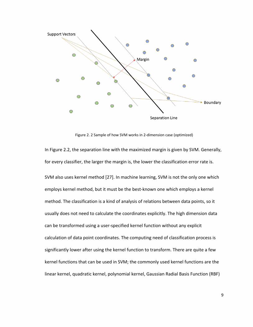
Figure 2. 2 Sample of how SVM works in 2-dimension case (optimized)

In Figure 2.2, the separation line with the maximized margin is given by SVM. Generally,

for every classifier, the larger the margin is, the lower the classification error rate is.

SVM also uses kernel method [27]. In machine learning, SVM is not the only one which

employs kernel method, but it must be the best-known one which employs a kernel

method. The classification is a kind of analysis of relations between data points, so it

usually does not need to calculate the coordinates explicitly. The high dimension data

can be transformed using a user-specified kernel function without any explicit

calculation of data point coordinates. The computing need of classification process is

significantly lower after using the kernel function to transform. There are quite a few

kernel functions that can be used in SVM; the commonly used kernel functions are the

linear kernel, quadratic kernel, polynomial kernel, Gaussian Radial Basis Function (RBF)

10

kernel, and Multilayer Perceptron (MLP) kernel. The RBF kernel is the most popular and

most commonly used one, and it is used in this study as well.

The inputs of an SVM classification algorithm in Matlab are called features. In this study,

all the inputs for SVM training or parameters tuning are constructed from technical

indicators (Tis) [28].

2.2 Technical Indicators (TIs)

There are 24 TIs used in testing, and almost all of them come from the Technical

Analysis Library (TA-lib). They are not equal to features, and features are made from

them. There are 44 features made from TIs [29], [30].

2.2.1 Relative Strength Index (RSI)

𝑅𝑅𝑅𝑅𝑅𝑅 = 100 −100

1 + 𝑅𝑅𝑅𝑅

Where RS is the average upward price change divided by the average of downward price

change over the same period.

RS compares the magnitude of recent gains and losses over a specified period,

measuring the price movement and the changing speed of securities. It is used to

identify the overbought/overvalued (>70) or oversold/undervalued (<30) status of

certain assets.

In our Matlab code, the function is “TA_RSI,” a 14-day period is used for RS.

11

2.2.2 Bollinger Bands

Bollinger Bands are used to measure the volatility of a stock price and involves an upper

and a lower band along with a simple moving average.

Bollinger Bands consist of:

• An N-period moving average

• An upper band at K times an N-period standard deviation above the moving

average

• A lower band at K times an N-period standard deviation below the moving

average

In our Matlab code, the function is “TA_BBANDS” and a 9-day period is used. Two times

the standard deviation is used to determine the upper and lower band.

2.2.3 Stochastic Oscillator

The Stochastic Oscillator compares closing price of a stock to the range of its price over

a specified period. This indicator includes two indicators: The Stochastic Fast (%K) and

the Stochastic Slow (%D). Their formulas are:

%𝐾𝐾 = 100𝐶𝐶 − 𝐿𝐿𝑁𝑁𝐻𝐻𝑁𝑁 − 𝐿𝐿𝑁𝑁

%𝐷𝐷 = 𝑀𝑀 𝑝𝑝𝑝𝑝𝑟𝑟𝑟𝑟𝑟𝑟𝑟𝑟 𝑅𝑅𝑀𝑀𝑆𝑆 𝑟𝑟𝑜𝑜 %𝐾𝐾

Where 𝐶𝐶 is closing price, 𝐿𝐿𝑁𝑁 is the lowest trading price of 14 previous trading days. 𝐻𝐻𝑁𝑁 is

the highest trading price of the 14 previous trading days. The SMA stands for Simple

12

Moving Average, which is explained below.

In our Matlab code, the function is “TA_STOCHF” and we use 𝑁𝑁 = 14 and 𝑀𝑀 = 3.

2.2.4 Simple Moving Average (SMA)

A Simple Moving Average (SMA) is an arithmetic moving average. The SMA is calculated

by adding up the total of closing prices of the security for a few periods and dividing this

sum by a pre-set number. Typically, the period is a day.

𝑅𝑅𝑀𝑀𝑆𝑆 = 𝑠𝑠𝑠𝑠𝑠𝑠 𝑟𝑟𝑜𝑜 𝑐𝑐𝑐𝑐𝑟𝑟𝑠𝑠𝑟𝑟𝑐𝑐𝑐𝑐 𝑝𝑝𝑟𝑟𝑟𝑟𝑐𝑐𝑝𝑝 𝑜𝑜𝑟𝑟𝑟𝑟 𝑁𝑁 𝑡𝑡𝑟𝑟𝑡𝑡𝑟𝑟𝑟𝑟𝑐𝑐𝑐𝑐 𝑟𝑟𝑡𝑡𝑑𝑑𝑠𝑠/𝑁𝑁

In our Matlab code, the function is “TA_SMA” and there are two sets of parameters

used: the 10-day SMA and the 21-day SMA.

2.2.5 Exponential Moving Average (EMA)

The Exponential Moving Average (EMA) is another moving average but is like a simple

moving average. The difference between EMA and SMA is that EMA weighs more recent

data more heavily than less recent data. Here is the formula:

𝐸𝐸𝑀𝑀𝑆𝑆𝑡𝑡𝑡𝑡𝑡𝑡𝑡𝑡𝑡𝑡 = 𝐶𝐶𝑡𝑡𝑡𝑡𝑡𝑡𝑡𝑡𝑡𝑡 ∗ 𝐾𝐾𝑁𝑁 + 𝐸𝐸𝑀𝑀𝑆𝑆𝑡𝑡𝑦𝑦𝑦𝑦𝑡𝑡𝑦𝑦𝑦𝑦𝑡𝑡𝑡𝑡𝑡𝑡 ∗ (1 − 𝐾𝐾𝑁𝑁)

Where 𝐶𝐶𝑡𝑡𝑡𝑡𝑡𝑡𝑡𝑡𝑡𝑡 is today’s closing price, 𝑁𝑁 is the length of 𝐸𝐸𝑀𝑀𝑆𝑆. For example, if it is 4-day

EMA, the N is 4. 𝐾𝐾𝑁𝑁 = 2/(𝑁𝑁 + 1), 𝐸𝐸𝑀𝑀𝑆𝑆𝑡𝑡𝑦𝑦𝑦𝑦𝑡𝑡𝑦𝑦𝑦𝑦𝑡𝑡𝑡𝑡𝑡𝑡 is the previous EMA value, calculated

using the same formula.

In our Matlab code, the function is “TA_EMA” and we use a 4-day EMA.

13

2.2.6 Triple Exponential Moving Average (TEMA)

Triple Exponential Moving Average (TEMA) is another moving average. It is a composite

of a single exponential moving average, a double exponential moving average, and a

triple exponential moving average. Here is the equation:

𝑇𝑇𝐸𝐸𝑀𝑀𝑆𝑆 = 3 ∗ 𝐸𝐸𝑀𝑀𝑆𝑆 − 3 ∗ 𝐸𝐸𝑀𝑀𝑆𝑆(𝐸𝐸𝑀𝑀𝑆𝑆) + 𝐸𝐸𝑀𝑀𝑆𝑆(𝐸𝐸𝑀𝑀𝑆𝑆(𝐸𝐸𝑀𝑀𝑆𝑆))

Compared to EMA, TEMA smooths price fluctuations and filters out volatility, making it

easier to identify trends with less lag time.

2.2.7 Kaufman Adaptive Moving Average (KAMA)

A moving average designed to account for market noise or volatility. It will closely follow

prices when the price swings are relatively small, and the noise is low. KAMA will also

adjust itself when the price swings, widens and follows price more loosely to keep it

smooth. Here is the equation:

𝐶𝐶𝑠𝑠𝑟𝑟𝑟𝑟𝑝𝑝𝑐𝑐𝑡𝑡 𝐾𝐾𝑆𝑆𝑀𝑀𝑆𝑆 = 𝑃𝑃𝑟𝑟𝑟𝑟𝑟𝑟𝑟𝑟 𝐾𝐾𝑆𝑆𝑀𝑀𝑆𝑆 + 𝑅𝑅𝐶𝐶 ∗ (𝑃𝑃𝑟𝑟𝑟𝑟𝑐𝑐𝑝𝑝 − 𝑃𝑃𝑟𝑟𝑟𝑟𝑟𝑟𝑟𝑟 𝐾𝐾𝑆𝑆𝑀𝑀𝑆𝑆)

SC is the Smoothing Constant which is calculated based on Efficiency Ratio (ER). ER is

basically when the price change is adjusted for the daily volatility. Here are the

equations:

𝐸𝐸𝑅𝑅 =𝑆𝑆𝐴𝐴𝑅𝑅�𝑐𝑐𝑐𝑐𝑟𝑟𝑠𝑠𝑝𝑝 𝑝𝑝𝑟𝑟𝑟𝑟𝑐𝑐𝑝𝑝 − 𝑐𝑐𝑐𝑐𝑟𝑟𝑠𝑠𝑝𝑝 𝑝𝑝𝑟𝑟𝑟𝑟𝑐𝑐𝑝𝑝(10 𝑝𝑝𝑝𝑝𝑟𝑟𝑟𝑟𝑟𝑟𝑟𝑟 𝑡𝑡𝑐𝑐𝑟𝑟)�

𝑣𝑣𝑟𝑟𝑐𝑐𝑡𝑡𝑡𝑡𝑟𝑟𝑐𝑐𝑟𝑟𝑡𝑡𝑑𝑑

𝑉𝑉𝑟𝑟𝑐𝑐𝑡𝑡𝑡𝑡𝑟𝑟𝑐𝑐𝑟𝑟𝑡𝑡𝑑𝑑 𝑟𝑟𝑠𝑠 𝑡𝑡ℎ𝑝𝑝 𝑠𝑠𝑠𝑠𝑠𝑠 𝑟𝑟𝑜𝑜 𝑡𝑡ℎ𝑝𝑝 𝑡𝑡𝑎𝑎𝑠𝑠𝑟𝑟𝑐𝑐𝑠𝑠𝑡𝑡𝑝𝑝 𝑣𝑣𝑡𝑡𝑐𝑐𝑠𝑠𝑝𝑝 𝑟𝑟𝑜𝑜 𝑡𝑡ℎ𝑝𝑝 𝑐𝑐𝑡𝑡𝑠𝑠𝑡𝑡 𝑡𝑡𝑝𝑝𝑐𝑐 𝑐𝑐𝑐𝑐𝑟𝑟𝑠𝑠𝑝𝑝 𝑝𝑝𝑟𝑟𝑟𝑟𝑐𝑐𝑝𝑝 𝑐𝑐ℎ𝑡𝑡𝑐𝑐𝑐𝑐𝑝𝑝𝑠𝑠

𝑅𝑅𝐶𝐶 = (𝐸𝐸𝑅𝑅 ∗ (𝑜𝑜𝑡𝑡𝑠𝑠𝑡𝑡𝑝𝑝𝑠𝑠𝑡𝑡 𝑅𝑅𝐶𝐶 − 𝑠𝑠𝑐𝑐𝑟𝑟𝑠𝑠𝑝𝑝𝑠𝑠𝑡𝑡 𝑅𝑅𝐶𝐶) + 𝑅𝑅𝑐𝑐𝑟𝑟𝑠𝑠𝑝𝑝𝑠𝑠𝑡𝑡 𝑅𝑅𝐶𝐶)2

14

Here we use KAMA (10, 2, 30). 10 is the number of periods for the ER, 2 is the number of

periods for the fastest EMA constant (fastest SC), 30 is the number of periods for the

slowest EMA constant (slowest SC).

2.2.8 Lowest Value & Highest Value over a Specified Period (Min & Max)

Those two technical indicators are merely the minimum and maximum value appearing

over a certain period.

In our Matlab code, the function is “TA_MIN” and “TA_MAX.” The period we used is a 5-

day period.

*2.2.8 introduces two TIs.

2.2.9 Connors RSI (CRSI)

Connors RSI has three major components: RSI, Updown Length, and ROC. RSI and ROC

are introduced separately in this Chapter. Updown Length is the number of consecutive

days that a security price has either closed up (higher than previous day) or closed down

(lower than previous days). We usually use closing price as default. Closing up is a

positive number, and closing down is a negative number.

CRSI has three variables, and here is the equation example for CRSI (3, 2, 100):

𝐶𝐶𝑅𝑅𝑅𝑅𝑅𝑅(3,2,100) =𝑅𝑅𝑅𝑅𝑅𝑅(3) + 𝑅𝑅𝑅𝑅𝑅𝑅(𝑈𝑈𝑝𝑝𝑟𝑟𝑟𝑟𝑠𝑠𝑐𝑐 𝐿𝐿𝑝𝑝𝑐𝑐𝑐𝑐𝑡𝑡ℎ, 2) + 𝑅𝑅𝑅𝑅𝐶𝐶(100)

3

15

3 is the number of periods for RSI, 2 is the number of periods for Up-Down Length, 100

is the number of periods for ROC.

2.2.10 Money Flow Index (MFI)

The Money Flow Index measures the inflow and outflow of money into certain securities

over a period. It uses a stock's price and volume to measure trading pressure.

Here are the steps/items used to calculate MFI:

𝑇𝑇𝑑𝑑𝑝𝑝𝑟𝑟𝑐𝑐𝑡𝑡𝑐𝑐 𝑝𝑝𝑟𝑟𝑟𝑟𝑐𝑐𝑝𝑝 = (ℎ𝑟𝑟𝑐𝑐ℎ 𝑝𝑝𝑟𝑟𝑟𝑟𝑐𝑐𝑝𝑝 + 𝑐𝑐𝑟𝑟𝑠𝑠 𝑝𝑝𝑟𝑟𝑟𝑟𝑐𝑐𝑝𝑝 + 𝑐𝑐𝑐𝑐𝑟𝑟𝑠𝑠𝑟𝑟𝑐𝑐𝑐𝑐 𝑝𝑝𝑟𝑟𝑟𝑟𝑐𝑐𝑝𝑝)/3

𝑅𝑅𝑡𝑡𝑠𝑠 𝑠𝑠𝑟𝑟𝑐𝑐𝑝𝑝𝑑𝑑 𝑜𝑜𝑐𝑐𝑟𝑟𝑠𝑠 = 𝑡𝑡𝑑𝑑𝑝𝑝𝑟𝑟𝑐𝑐𝑡𝑡𝑐𝑐 𝑝𝑝𝑟𝑟𝑟𝑟𝑐𝑐𝑝𝑝 ∗ 𝑣𝑣𝑟𝑟𝑐𝑐𝑠𝑠𝑠𝑠𝑝𝑝

𝑀𝑀𝑟𝑟𝑐𝑐𝑝𝑝𝑑𝑑 𝑜𝑜𝑐𝑐𝑟𝑟𝑠𝑠 𝑟𝑟𝑡𝑡𝑡𝑡𝑟𝑟𝑟𝑟 = (14 − 𝑟𝑟𝑡𝑡𝑑𝑑 𝑃𝑃𝑟𝑟𝑠𝑠𝑟𝑟𝑡𝑡𝑟𝑟𝑣𝑣𝑝𝑝 𝑀𝑀𝑟𝑟𝑐𝑐𝑝𝑝𝑑𝑑 𝐹𝐹𝑐𝑐𝑟𝑟𝑠𝑠)/(14 − 𝑟𝑟𝑡𝑡𝑑𝑑 𝑁𝑁𝑝𝑝𝑐𝑐𝑡𝑡𝑡𝑡𝑟𝑟𝑣𝑣𝑝𝑝 𝑀𝑀𝑟𝑟𝑐𝑐𝑝𝑝𝑑𝑑 𝐹𝐹𝑐𝑐𝑟𝑟𝑠𝑠)

𝑀𝑀𝐹𝐹𝑅𝑅 = 100 −100

1 −𝑀𝑀𝑟𝑟𝑐𝑐𝑝𝑝𝑑𝑑 𝑜𝑜𝑐𝑐𝑟𝑟𝑠𝑠 𝑟𝑟𝑡𝑡𝑡𝑡𝑟𝑟𝑟𝑟

In our Matlab code, the function is “TA_MFI,” and the function requires high, low,

closing prices and volumes. No other parameter (number) is needed as input.

2.2.11 Balance of Power (BOP)

The Balance of Power (BOP) is designed to measure the strength of buyers versus sellers

by assessing the ability of each to push the price to an extreme level.

𝐴𝐴𝑅𝑅𝑃𝑃 = (𝑐𝑐𝑐𝑐𝑟𝑟𝑠𝑠𝑟𝑟𝑐𝑐𝑐𝑐 𝑝𝑝𝑟𝑟𝑟𝑟𝑐𝑐𝑝𝑝 − 𝑟𝑟𝑝𝑝𝑝𝑝𝑐𝑐𝑟𝑟𝑐𝑐𝑐𝑐 𝑝𝑝𝑟𝑟𝑟𝑟𝑐𝑐𝑝𝑝)/(ℎ𝑟𝑟𝑐𝑐ℎ 𝑝𝑝𝑟𝑟𝑟𝑟𝑐𝑐𝑝𝑝 − 𝑐𝑐𝑟𝑟𝑠𝑠 𝑝𝑝𝑟𝑟𝑟𝑟𝑐𝑐𝑝𝑝)

16

No other parameter/number is needed besides close, open, high, and low prices.

In our Matlab code, the function is “TA_BOP.”

2.2.12 Williams %R (WPR)

Williams %R is also referred to as the Williams Percent Range (WPR). It also measures

overbought and oversold levels. The equation is:

%𝑅𝑅 =(ℎ𝑟𝑟𝑐𝑐ℎ 𝑝𝑝𝑟𝑟𝑟𝑟𝑐𝑐𝑝𝑝 − 𝑐𝑐𝑐𝑐𝑟𝑟𝑠𝑠𝑟𝑟𝑐𝑐𝑐𝑐 𝑝𝑝𝑟𝑟𝑟𝑟𝑐𝑐𝑝𝑝)

ℎ𝑟𝑟𝑐𝑐ℎ 𝑝𝑝𝑟𝑟𝑟𝑟𝑐𝑐𝑝𝑝 − 𝑐𝑐𝑟𝑟𝑠𝑠 𝑝𝑝𝑟𝑟𝑟𝑟𝑐𝑐𝑝𝑝∗ −100

In our Matlab code, the function is “TA_WILLR.” No other parameter/number is needed

besides high, low, and closing prices.

2.2.13 Ultimate Oscillator (ULT)

Ultimate Oscillator is a range-bound indicator. It uses the weighted average of three

different periods to reduce volatility and false transaction signals. Before calculating

ULT, we need to define several items:

𝑡𝑡𝑟𝑟𝑠𝑠𝑝𝑝 𝑐𝑐𝑟𝑟𝑠𝑠 = min(𝑐𝑐𝑟𝑟𝑠𝑠 𝑝𝑝𝑟𝑟𝑟𝑟𝑐𝑐𝑝𝑝, 𝑝𝑝𝑟𝑟𝑝𝑝𝑣𝑣𝑟𝑟𝑟𝑟𝑠𝑠𝑠𝑠 𝑐𝑐𝑐𝑐𝑟𝑟𝑠𝑠𝑟𝑟𝑐𝑐𝑐𝑐 𝑝𝑝𝑟𝑟𝑟𝑟𝑐𝑐𝑝𝑝 )

𝑡𝑡𝑟𝑟𝑠𝑠𝑝𝑝 ℎ𝑟𝑟𝑐𝑐ℎ = max(ℎ𝑟𝑟𝑐𝑐ℎ 𝑝𝑝𝑟𝑟𝑟𝑟𝑐𝑐𝑝𝑝,𝑝𝑝𝑟𝑟𝑝𝑝𝑣𝑣𝑟𝑟𝑟𝑟𝑠𝑠𝑠𝑠 𝑐𝑐𝑐𝑐𝑟𝑟𝑠𝑠𝑟𝑟𝑐𝑐𝑐𝑐 𝑝𝑝𝑟𝑟𝑟𝑟𝑐𝑐𝑝𝑝)

𝑎𝑎𝑠𝑠𝑑𝑑𝑟𝑟𝑐𝑐𝑐𝑐 𝑝𝑝𝑟𝑟𝑝𝑝𝑠𝑠𝑠𝑠𝑠𝑠𝑟𝑟𝑝𝑝(𝑎𝑎𝑝𝑝) = 𝑐𝑐𝑐𝑐𝑟𝑟𝑠𝑠𝑝𝑝 − 𝑡𝑡𝑟𝑟𝑠𝑠𝑝𝑝 𝑐𝑐𝑟𝑟𝑠𝑠

𝑡𝑡𝑟𝑟𝑠𝑠𝑝𝑝 𝑟𝑟𝑡𝑡𝑐𝑐𝑐𝑐𝑝𝑝(𝑡𝑡𝑟𝑟) = 𝑡𝑡𝑟𝑟𝑠𝑠𝑝𝑝 ℎ𝑟𝑟𝑐𝑐ℎ − 𝑡𝑡𝑟𝑟𝑠𝑠𝑝𝑝 𝑐𝑐𝑟𝑟𝑠𝑠

𝑡𝑡𝑣𝑣𝑐𝑐7 =𝑎𝑎𝑝𝑝1 + 𝑎𝑎𝑝𝑝2 + ⋯+ 𝑎𝑎𝑝𝑝7𝑡𝑡𝑟𝑟1 + 𝑡𝑡𝑟𝑟2 + ⋯+ 𝑡𝑡𝑟𝑟7

17

Where 𝑡𝑡𝑣𝑣𝑐𝑐7 is the sum of buying pressure over the most recent seven days divided by

the sum of true range over those seven days. The same calculation applies to 𝑡𝑡𝑣𝑣𝑐𝑐14 and

𝑡𝑡𝑣𝑣𝑐𝑐, and the ULT is:

𝑈𝑈𝐿𝐿𝑇𝑇 = 100 ∗4 ∗ 𝑡𝑡𝑣𝑣𝑐𝑐7 + 2 ∗ 𝑡𝑡𝑣𝑣𝑐𝑐14 + 𝑡𝑡𝑣𝑣𝑐𝑐28

4 + 2 + 1

In our Matlab code, the function is “TA_ULTOSC.” The period for the three averages in

ULT calculation is adjustable. However, our setting for the three averages is the same as

the example: 7, 14, and 28.

2.2.14 Rate of Change (ROC)

The Rate of Change (ROC) is the speed at which a variable will change over time. Here,

ROC is used to describe the percentage of change in the value of a stock over a period.

The equation is:

𝑅𝑅𝑅𝑅𝐶𝐶 = �𝑐𝑐𝑠𝑠𝑟𝑟𝑟𝑟𝑝𝑝𝑐𝑐𝑡𝑡 𝑣𝑣𝑡𝑡𝑐𝑐𝑠𝑠𝑝𝑝

𝑁𝑁 − 𝑟𝑟𝑡𝑡𝑑𝑑 𝑝𝑝𝑟𝑟𝑝𝑝𝑣𝑣𝑟𝑟𝑟𝑟𝑠𝑠𝑠𝑠 𝑣𝑣𝑡𝑡𝑐𝑐𝑠𝑠𝑝𝑝− 1� ∗ 100

In our Matlab code, the function is “TA_ROC.” We use closing price as the value of a

stock and let 𝑁𝑁 = 5.

2.2.15 Average True Range (ATR) & Normalized Average True Range (NATR)

The Average True Range (ATR) is a measure of volatility. Before we calculate ATR, we

define the true range as the following:

𝑡𝑡𝑟𝑟𝑠𝑠𝑝𝑝 𝑟𝑟𝑡𝑡𝑐𝑐𝑐𝑐𝑝𝑝 (𝑇𝑇𝑅𝑅) = 𝑠𝑠𝑡𝑡𝑚𝑚(ℎ𝑟𝑟𝑐𝑐ℎ − 𝑐𝑐𝑟𝑟𝑠𝑠,𝑡𝑡𝑎𝑎𝑠𝑠(ℎ𝑟𝑟𝑐𝑐ℎ − 𝑝𝑝𝑟𝑟𝑝𝑝𝑣𝑣 𝑐𝑐𝑐𝑐𝑟𝑟𝑠𝑠𝑟𝑟𝑐𝑐𝑐𝑐),𝑡𝑡𝑎𝑎𝑠𝑠(𝑐𝑐𝑟𝑟𝑠𝑠 − 𝑝𝑝𝑟𝑟𝑝𝑝𝑣𝑣 𝑐𝑐𝑐𝑐𝑟𝑟𝑠𝑠𝑟𝑟𝑐𝑐𝑐𝑐)

Where the high, low, prev close are high, low, and previous closing prices.

18

The ATR is a moving average of the true ranges. The following is the ATR form of the

exponential moving average:

𝑆𝑆𝑇𝑇𝑅𝑅𝑡𝑡𝑡𝑡𝑡𝑡𝑡𝑡𝑡𝑡 =𝑆𝑆𝑇𝑇𝑅𝑅𝑡𝑡𝑦𝑦𝑦𝑦𝑡𝑡𝑦𝑦𝑦𝑦𝑡𝑡𝑡𝑡𝑡𝑡 ∗ (𝑁𝑁 − 1) + 𝑡𝑡𝑟𝑟𝑠𝑠𝑝𝑝 𝑟𝑟𝑡𝑡𝑐𝑐𝑐𝑐𝑝𝑝𝑡𝑡𝑡𝑡𝑡𝑡𝑡𝑡𝑡𝑡

𝑁𝑁

Where N is the length of the moving average.

For the Normalized Average True Range (NATR), the formula is:

𝑁𝑁𝑆𝑆𝑇𝑇𝑅𝑅 =𝑆𝑆𝑇𝑇𝑅𝑅𝑁𝑁

𝑐𝑐𝑐𝑐𝑟𝑟𝑠𝑠𝑟𝑟𝑐𝑐𝑐𝑐 𝑝𝑝𝑟𝑟𝑟𝑟𝑐𝑐𝑝𝑝∗ 100

In our Matlab code, the functions are “TA_ATR” and TA_NATR.” We use 𝑁𝑁 = 14 as

suggested.

*2.2.15 introduces two Technical Indicators.

2.2.16 Standard Deviation (SD)

Standard Deviation (SD) is a fundamental measurement in descriptive statistics. SD

measures the dispersion of a set of data from its mean. In investment, SD measures the

volatility of the investments.

In our Matlab code, the function is “TA_STDDEV,” and we calculate SD based on closing

price and set the number of variable equals to 7.

19

2.2.17 On-Balance Volume (OBV)

On-Balance Volume is a momentum indicator that uses volume flow to predict changes

in stock price. It is believed by the creator of the indicator that sharp increases in

volume without a significant change in stock price will eventually lead to a jump forward

in the price and vice versa.

The calculation of OBV is a running total of positive and negative trading volume for a

stock. If today’s closing price is above yesterday’s closing price, today’s trading volume is

positive and 𝑅𝑅𝐴𝐴𝑉𝑉𝑡𝑡𝑡𝑡𝑡𝑡𝑡𝑡𝑡𝑡 = 𝑅𝑅𝐴𝐴𝑉𝑉𝑡𝑡𝑦𝑦𝑦𝑦𝑡𝑡𝑦𝑦𝑦𝑦𝑡𝑡𝑡𝑡𝑡𝑡 − 𝑇𝑇𝑟𝑟𝑟𝑟𝑡𝑡𝑑𝑑′𝑠𝑠 𝑡𝑡𝑟𝑟𝑡𝑡𝑟𝑟𝑟𝑟𝑐𝑐𝑐𝑐 𝑣𝑣𝑟𝑟𝑐𝑐𝑠𝑠𝑠𝑠𝑝𝑝; if today’s closing

price is below yesterday’s closing price, today’s trading volume is negative and

𝑅𝑅𝐴𝐴𝑉𝑉𝑡𝑡𝑡𝑡𝑡𝑡𝑡𝑡𝑡𝑡 = 𝑅𝑅𝐴𝐴𝑉𝑉𝑡𝑡𝑦𝑦𝑦𝑦𝑡𝑡𝑦𝑦𝑦𝑦𝑡𝑡𝑡𝑡𝑡𝑡 − 𝑇𝑇𝑟𝑟𝑟𝑟𝑡𝑡𝑑𝑑′𝑠𝑠 𝑡𝑡𝑟𝑟𝑡𝑡𝑟𝑟𝑟𝑟𝑐𝑐𝑐𝑐 𝑣𝑣𝑟𝑟𝑐𝑐𝑠𝑠𝑠𝑠𝑝𝑝.

In our Matlab code, the function is “TA_OBV” and there is no other parameter/number

needed besides closing price and volume.

2.2.18 Percentage Price Oscillator (PPO)

Percentage Price Oscillator (PPO) is a momentum indicator that shows the relationship

between two moving averages. Commonly, exponential moving averages are used in

PPO. Here is the equation for PPO in terms of EMAs as an example:

𝑃𝑃𝑃𝑃𝑅𝑅 =𝐸𝐸𝑀𝑀𝑆𝑆𝑁𝑁 − 𝐸𝐸𝑀𝑀𝑆𝑆𝑀𝑀

𝐸𝐸𝑀𝑀𝑆𝑆𝑀𝑀

Where N is a smaller number compared with M, 𝐸𝐸𝑀𝑀𝑆𝑆𝑁𝑁 is a faster, short-term EMA and

𝐸𝐸𝑀𝑀𝑆𝑆𝑀𝑀 is a slower, long-term EMA. Usually, N is 9 and M is 26.

20

In this Matlab code, the function is "TA_PPO" and we use 𝑁𝑁 = 9 𝑡𝑡𝑐𝑐𝑟𝑟 𝑀𝑀 = 26. Besides

N & M, there is another parameter which is needed to set: the type of moving average.

We use two which stands for exponential moving average form.

2.2.19 Median Price

The median price is merely the mid-point of a trading range for a period. It is an

arithmetic average. The formula is:

𝑀𝑀𝑝𝑝𝑟𝑟𝑟𝑟𝑡𝑡𝑐𝑐 𝑃𝑃𝑟𝑟𝑟𝑟𝑐𝑐𝑝𝑝 =ℎ𝑟𝑟𝑐𝑐ℎ 𝑝𝑝𝑟𝑟𝑟𝑟𝑐𝑐𝑝𝑝 + 𝑐𝑐𝑟𝑟𝑠𝑠 𝑝𝑝𝑟𝑟𝑟𝑟𝑐𝑐𝑝𝑝

2

In our Matlab code, the function is “TA_MEDPRICE” and there is no other

parameter/number needed besides high and low price.

2.2.20 Average Directional Index (ADX)

The Average Index is used to qualify trend strength. It is a combination of two

indicators: the Positive Directional Indicator (+DI) and the Negative Directional Indicator

(-DI). To calculate +DI or -DI, we need to calculate the directional movement first (+DM

or -DM):

𝑈𝑈𝑝𝑝𝑀𝑀𝑟𝑟𝑣𝑣𝑝𝑝 = 𝑡𝑡𝑟𝑟𝑟𝑟𝑡𝑡𝑑𝑑′𝑠𝑠 ℎ𝑟𝑟𝑐𝑐ℎ − 𝑑𝑑𝑝𝑝𝑠𝑠𝑡𝑡𝑝𝑝𝑟𝑟𝑟𝑟𝑡𝑡𝑑𝑑′𝑠𝑠 ℎ𝑟𝑟𝑐𝑐ℎ

𝐷𝐷𝑟𝑟𝑠𝑠𝑐𝑐𝑀𝑀𝑟𝑟𝑣𝑣𝑝𝑝 = 𝑑𝑑𝑝𝑝𝑠𝑠𝑡𝑡𝑝𝑝𝑟𝑟𝑟𝑟𝑡𝑡𝑑𝑑′𝑠𝑠 𝑐𝑐𝑟𝑟𝑠𝑠 − 𝑡𝑡𝑟𝑟𝑟𝑟𝑡𝑡𝑑𝑑′𝑠𝑠 𝑐𝑐𝑟𝑟𝑠𝑠

𝑟𝑟𝑜𝑜 𝑈𝑈𝑝𝑝𝑀𝑀𝑟𝑟𝑣𝑣𝑝𝑝 > 𝐷𝐷𝑟𝑟𝑠𝑠𝑐𝑐𝑀𝑀𝑟𝑟𝑣𝑣𝑝𝑝 𝑡𝑡𝑐𝑐𝑟𝑟 𝑈𝑈𝑝𝑝𝑀𝑀𝑟𝑟𝑣𝑣𝑝𝑝 > 0, 𝑡𝑡ℎ𝑝𝑝𝑐𝑐 + 𝐷𝐷𝑀𝑀 = 𝑈𝑈𝑝𝑝𝑀𝑀𝑟𝑟𝑣𝑣𝑝𝑝, 𝑝𝑝𝑐𝑐𝑠𝑠𝑝𝑝 + 𝐷𝐷𝑀𝑀 = 0

𝑟𝑟𝑜𝑜 𝐷𝐷𝑟𝑟𝑠𝑠𝑐𝑐𝑀𝑀𝑟𝑟𝑣𝑣𝑝𝑝 > 𝑈𝑈𝑝𝑝𝑀𝑀𝑟𝑟𝑣𝑣𝑝𝑝 𝑡𝑡𝑐𝑐𝑟𝑟 𝐷𝐷𝑟𝑟𝑠𝑠𝑐𝑐𝑀𝑀𝑟𝑟𝑣𝑣𝑝𝑝 > 0, 𝑡𝑡ℎ𝑝𝑝𝑐𝑐 − 𝐷𝐷𝑀𝑀

= 𝐷𝐷𝑟𝑟𝑠𝑠𝑐𝑐𝑀𝑀𝑟𝑟𝑣𝑣𝑝𝑝, 𝑝𝑝𝑐𝑐𝑠𝑠𝑝𝑝 − 𝐷𝐷𝑀𝑀 = 0

21

After +DM and -DM are calculated, +DI and -DI are:

+𝐷𝐷𝑅𝑅 = 100 ∗𝑅𝑅𝑀𝑀𝑆𝑆𝑁𝑁(+𝐷𝐷𝑀𝑀)

𝑆𝑆𝑇𝑇𝑅𝑅

−𝐷𝐷𝑅𝑅 = 100 ∗�𝑅𝑅𝑀𝑀𝑆𝑆𝑁𝑁(−𝐷𝐷𝑀𝑀)�

𝑆𝑆𝑇𝑇𝑅𝑅

Then the ADX is:

𝑆𝑆𝐷𝐷𝐴𝐴 = 100 ∗ 𝑅𝑅𝑀𝑀𝑆𝑆𝑁𝑁(𝑡𝑡𝑎𝑎𝑠𝑠(+𝐷𝐷𝑅𝑅 − (−𝐷𝐷𝑅𝑅)+𝐷𝐷𝑅𝑅 + (−𝐷𝐷𝑅𝑅)

)

In our Matlab code, the function is “TA_ADX,” and we use 𝑁𝑁 = 14.

2.2.21 Chande Momentum Oscillator (CMO)

Like RSI, the indicator is also used to measure the oversold (+50) or overbought (-50)

status of certain securities. To get the number, first, we calculate the difference

between the total of recent gains and the total of recent losses over a period. Then, we

divide the difference by the total price movement over the same period. Let's define the

total of gain, loss, and price movement:

𝑟𝑟𝑜𝑜 𝑐𝑐𝑐𝑐𝑟𝑟𝑠𝑠𝑟𝑟𝑐𝑐𝑐𝑐𝑡𝑡𝑡𝑡𝑡𝑡𝑡𝑡𝑡𝑡 − 𝑐𝑐𝑐𝑐𝑟𝑟𝑠𝑠𝑟𝑟𝑐𝑐𝑐𝑐𝑡𝑡𝑦𝑦𝑦𝑦𝑡𝑡𝑦𝑦𝑦𝑦𝑡𝑡𝑡𝑡𝑡𝑡

> 0, 𝑡𝑡ℎ𝑝𝑝𝑐𝑐 𝑐𝑐𝑐𝑐𝑟𝑟𝑠𝑠𝑟𝑟𝑐𝑐𝑐𝑐𝑡𝑡𝑡𝑡𝑡𝑡𝑡𝑡𝑡𝑡 − 𝑐𝑐𝑐𝑐𝑟𝑟𝑠𝑠𝑟𝑟𝑐𝑐𝑐𝑐𝑡𝑡𝑦𝑦𝑦𝑦𝑡𝑡𝑦𝑦𝑦𝑦𝑡𝑡𝑡𝑡𝑡𝑡 𝑟𝑟𝑠𝑠 𝑐𝑐𝑡𝑡𝑟𝑟𝑐𝑐.

𝑟𝑟𝑜𝑜 𝑐𝑐𝑐𝑐𝑟𝑟𝑠𝑠𝑟𝑟𝑐𝑐𝑐𝑐𝑡𝑡𝑡𝑡𝑡𝑡𝑡𝑡𝑡𝑡 − 𝑐𝑐𝑐𝑐𝑟𝑟𝑠𝑠𝑟𝑟𝑐𝑐𝑐𝑐𝑡𝑡𝑦𝑦𝑦𝑦𝑡𝑡𝑦𝑦𝑦𝑦𝑡𝑡𝑡𝑡𝑡𝑡

< 0, 𝑡𝑡ℎ𝑝𝑝𝑐𝑐 𝑡𝑡𝑎𝑎𝑠𝑠(𝑐𝑐𝑐𝑐𝑟𝑟𝑠𝑠𝑟𝑟𝑐𝑐𝑐𝑐𝑡𝑡𝑡𝑡𝑡𝑡𝑡𝑡𝑡𝑡 − 𝑐𝑐𝑐𝑐𝑟𝑟𝑠𝑠𝑟𝑟𝑐𝑐𝑐𝑐𝑡𝑡𝑦𝑦𝑦𝑦𝑡𝑡𝑦𝑦𝑦𝑦𝑡𝑡𝑡𝑡𝑡𝑡) 𝑟𝑟𝑠𝑠 𝑐𝑐𝑟𝑟𝑠𝑠𝑠𝑠.

𝑡𝑡𝑟𝑟𝑡𝑡𝑡𝑡𝑐𝑐 𝑟𝑟𝑜𝑜 𝑐𝑐𝑡𝑡𝑟𝑟𝑐𝑐𝑠𝑠 = 𝑠𝑠𝑠𝑠𝑠𝑠𝑁𝑁(𝑐𝑐𝑡𝑡𝑟𝑟𝑐𝑐), 𝑡𝑡𝑟𝑟𝑡𝑡𝑡𝑡𝑐𝑐 𝑟𝑟𝑜𝑜 𝑐𝑐𝑟𝑟𝑠𝑠𝑠𝑠𝑝𝑝𝑠𝑠 = 𝑠𝑠𝑠𝑠𝑠𝑠𝑁𝑁(𝑐𝑐𝑟𝑟𝑠𝑠𝑠𝑠)

𝑝𝑝𝑟𝑟𝑟𝑟𝑐𝑐𝑝𝑝 𝑠𝑠𝑟𝑟𝑣𝑣𝑝𝑝𝑠𝑠𝑝𝑝𝑐𝑐𝑡𝑡 = 𝑡𝑡𝑟𝑟𝑡𝑡𝑡𝑡𝑐𝑐 𝑟𝑟𝑜𝑜 𝑐𝑐𝑡𝑡𝑟𝑟𝑐𝑐𝑠𝑠 + 𝑡𝑡𝑟𝑟𝑡𝑡𝑡𝑡𝑐𝑐 𝑟𝑟𝑜𝑜 𝑐𝑐𝑟𝑟𝑠𝑠𝑠𝑠𝑝𝑝𝑠𝑠

22

𝐶𝐶𝑀𝑀𝑅𝑅 = 100 ∗𝑠𝑠𝑠𝑠𝑠𝑠𝑁𝑁(𝑐𝑐𝑡𝑡𝑟𝑟𝑐𝑐) − 𝑠𝑠𝑠𝑠𝑠𝑠𝑁𝑁(𝑐𝑐𝑟𝑟𝑠𝑠𝑠𝑠)𝑠𝑠𝑠𝑠𝑠𝑠𝑁𝑁(𝑐𝑐𝑡𝑡𝑟𝑟𝑐𝑐) + 𝑠𝑠𝑠𝑠𝑠𝑠𝑁𝑁(𝑐𝑐𝑟𝑟𝑠𝑠𝑠𝑠)

Where N is the period, for example, a 10-day period.

In our Matlab code, the function is “TA_CMO” and we use 𝑁𝑁 = 10.

2.2.22 Commodity Channel Index (CCI)

The Commodity Channel Index (CCI) is an oscillator and is used to measure whether a

stock is oversold/overbought. It attains value by quantifying the relationship between

the stock’s typical price (𝑃𝑃𝑡𝑡), the N simple moving average of the stock’s typical

price (𝑅𝑅𝑀𝑀𝑆𝑆𝑁𝑁(𝑃𝑃𝑡𝑡)), and the N points mean absolute deviation from typical

price�𝜎𝜎𝑁𝑁(𝑃𝑃𝑡𝑡)�. Here is the formula:

𝐶𝐶𝐶𝐶𝑅𝑅 =𝑃𝑃𝑡𝑡 − 𝑅𝑅𝑀𝑀𝑆𝑆𝑁𝑁(𝑃𝑃𝑡𝑡)0.015 ∗ 𝜎𝜎𝑁𝑁(𝑃𝑃𝑡𝑡)

Where the typical price is 𝑃𝑃𝑡𝑡 = ℎ𝑖𝑖𝑖𝑖ℎ+𝑙𝑙𝑡𝑡𝑙𝑙+𝑐𝑐𝑙𝑙𝑡𝑡𝑦𝑦𝑖𝑖𝑐𝑐𝑖𝑖3

, and the aim of scaling by 1/0.015 is to

produce a more readable number.

In our Matlab code, the function is “TA_CCI”, and we use 𝑁𝑁 = 20.

2.3 Hypothesis

Although the financial market is complex, based on previous research, market trends

are somewhat predictable. The TA method offers a unique way to discover the secret of

future movement. A machine learning classifier such as SVM is a great tool that

significantly improves market trend prediction. An SVM based TA for market trend

prediction is a beautiful approach, and we believe it is possible to improve the

23

predicting accuracy by performing features selection while preparing training data for

an SVM based prediction model. Furthermore, improvement of the feature selection

algorithm can promote the prediction accuracy of the model again.

2.4 Goal

The goals of the work include:

1. Study prediction accuracy improvement after applying Sequential Feature

Selection function to an SVM based model.

We will use a fixed, initial combination of technical indicators as input to train

SVM and test the model. Then we apply ERFS on the same initial combination of

technical indicators, using the left indicators to train SVM and test the model.

The differences between the two groups of results will be studied.

2. We will apply the AHCele instead of the ERFS and repeat the test. The new group

of results is then studied and compared to the previous two result groups. The

differences will then be interpreted.

2.5 Evaluation Method

The critical measurement of the prediction model is the prediction accuracy, and all

results are finally evaluated by their prediction accuracy. The prediction model is trained

and tested/simulated based on historical data using Matlab. The classifier used for

predicting target is SVM. The prediction accuracy is defined as the sum of correctly

classified targets divided by the sum number of targets.

24

Chapter 3 Experiment Design

The whole experiment is carried out in Matlab based on its easily accessible and

powerful simulator. The market prediction is basically an application of the SVM

classifier. The data used to train the SVM classifier include features made from technical

indicators based on historical data from the S&P500 (^GSPC). Later we will use the

SP500 instead of the S&P500 (^GSPC). The trained SVM classifier is also tested on

historical data from the SP500.

3.1 Data Construction

The original data is historical S&P 500 index prices (^GSPC) acquired from Yahoo!

Finance. The available data spans from 1950 to 2017. This data is composed of daily

data points. Each data point consists of high, low, close, and open prices and volume of

a particular trading day. All the 24 technical indicators introduced in Chapter 2 are

calculated based on the market high, low, close, and open prices and volume and are

further made into 44 features. The features are the inputs for SVM training. Although

other indicator types are prepared, such as microeconomic indicators (other stocks'

momentum and acceleration) and microeconomic indicators, they were not used in our

experiments.

Among the 67 years of data, we take a 10-year window divided into two parts –the first

part is for the training aim, called In-Sample data; the second part is for the testing aim,

called Out-Of-Sample data. The length ratio of In-Sample data to the length of Out-Of-

25

Sample data is 7:3. The In-Sample is used for features selecting, and the data after

selection are for SVM training inputs. The Out-Of-Sample part is used for testing the

trained SVM classifier and returns a prediction accuracy used to evaluate the trained

model. There are approximately 252 trading days in a year, which makes about 1800

points in the In-Sample data and 800 points in the Out-Of-Sample data when daily data

is used.

In the following experiments, four pieces of data are used: 2007-2017, 2000-2010, 1992-

2001, and 1960-1970.

3.2 Classification

The prediction model is designed to indicate the market trend; it is the movement of the

S&P 500 index price in this case. All the data used as inputs are sharing the same unit:

the U.S. dollar. Based on the above information, the classification criterion is to check

the difference between the present index closing price and the previous index closing

price. If the difference is non-negative (including 0), which means the index closing price

does not fall, the classification result and record is a 1; if the difference is negative,

which means the index closing prices fall, the classification result and record is a 0.

3.3 Data Pre-processing

3.3.1 Interpolation

It is a necessary process before the data enters into the SVM. Due to missing values in

stock prices (or/and character of feature formulas), some "not a number" (NaN) values

appear, which can break SVM training rules and ruin the training process. Those NaN

26

values are converted into zeros in all following experiments to make the SVM work

normally. There is another way to interpolate these kinds of numbers using linear

regression or the average of several neighboring numbers to smooth out the holes.

Typically, this method eliminates the holes inside the training data more smoothly than

inserting zeros. However, when there is a string of NaN values, especially when starting

from the very beginning of the array, this method will not work well.

3.3.2 Normalization

After features are calculated, the magnitude order of features could be very different.

Some range from 0 to 1 or -1 to 1, while others range from 1 to 10,000. Their scales can

be incredibly different and will likely poorly affect the performance of the classifier,

which is trained via this data. It will significantly lengthen the running time of classifier

training. One reason is the mixed use of prices and volumes. Prices are recorded in the

hundreds or thousands of levels, but volumes are recorded in tens of millions. The other

reason is that all kinds of technical indicators are employed, some are designed to

determine percentages, and some are designed to determine large numbers. It is

essential to implement normalization to make the data organized and efficient. The

Matlab function "zscore", which performs better than another two choices "normc" and

"normalize", according to a summing-up in a similar work [31], is used in here to

normalize all the data.

With the character of each technical indicator/feature formula known, there is another

to avoid normalization while keeping data efficient. We can rescale each

27

indicator/feature to let their order of magnitude become more consistent before

pouring them into the SVM. This idea is tested and discussed separately at the end.

3.4 Feature Selection

3.4.1 General

Feature selection (FS) is a great way to screen data and improve the accuracy of a

prediction model [32]. Feature selection is a critical part of the following experiments.

The experiment designed a comparison among one control group and two experimental

groups. All three codes, including raw data processing, features calculating, and SVM

training, testing, and generating output, are the same except for feature selection parts.

For feature selection part, each group used different strategies.

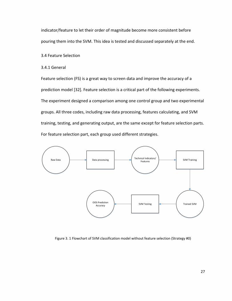
Data processingRaw Data Technical Indicators/Features

Trained SVM

SVM Training

SVM TestingOOS Prediction Accuracy

Figure 3. 1 Flowchart of SVM classification model without feature selection (Strategy #0)

28

3.4.2 Control Group – Strategy #0

The flowchart of the code used in the control group is given above. We call this Strategy

#0 (Without FS). Basically, the code in Strategy #0 includes no feature selection

algorithm. It just merely uses all initial features as input for SVM training.

First, the code acquires raw data from a prepared Excel file created directly by Yahoo!

Finance. The Excel document (.csv format) is the historical S&P 500 ^GSPC daily data

beginning in 1950, including open price, high price, low price, closing price, and daily

trading volume. Second, all the raw data goes into processing algorithm. All the data will

be extracted and separately stored. Date format will be changed, and step size

(prediction horizon) will be set. All 24 technical indicators will be calculated, and further

calculation is conducted to get all 44 initial features' values from the technical

indicators. Data piece boundaries will be set, and training and supervising groups will be

created. Third, after data processing, the prepared features input will be used in training

the SVM, and the trained SVM classifier will be employed as our prediction model. Last,

the testing group data created in the above step will be used to get the Out-of-Sample

prediction accuracies, which we will use to evaluate the effectiveness of the prediction

model.

29

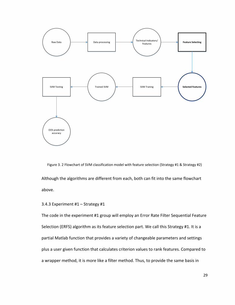
Data processingRaw Data Technical Indicators/Features

Selected Features

Feature Selecting

SVM TraningTrained SVMSVM Testing

OOS prediction accuracy

Figure 3. 2 Flowchart of SVM classification model with feature selection (Strategy #1 & Strategy #2)

Although the algorithms are different from each, both can fit into the same flowchart

above.

3.4.3 Experiment #1 – Strategy #1

The code in the experiment #1 group will employ an Error Rate Filter Sequential Feature

Selection (ERFS) algorithm as its feature selection part. We call this Strategy #1. It is a

partial Matlab function that provides a variety of changeable parameters and settings

plus a user given function that calculates criterion values to rank features. Compared to

a wrapper method, it is more like a filter method. Thus, to provide the same basis in

30

comparison, a piece of code is added to transform it into a wrapper method. Besides

features selection, all parameters and settings are the same as in any of the

experiments. The following is the flowchart of Strategy #1 feature selection following

the detailed introduction of Strategy #1.

Ranking by criterion value for every

combination of 1 feature/Saving index of

best feature into set

Features/Function/Setting number of

features to choose: 1(initial set: empyt)

Features/Function/Setting number of

features to choose: 2 (initial set: include feature selected in

previous round)

Ranking again for every combination of 2

features/Saving indices into set

Repeated 44 times with the same setting except “number of features to choose” varying from 1 to 44, saving 44 indices into the set. (the order of the indices is

the order of ranking)Final Ranking

Grouped all features into 44 groups of feature according to ranking, first group with only first ranking feature, second group with first and second ranking features, …...last group with all 44 features. Test In-Sample prediction accuracies of all 44 groups based on training (In-Sample) data, choose the a group with highest In-Sample accuracy, save the feature indices and In-Sample prediction accuracy

Best combination of features

Figure 3. 3 Flowchart of feature selection (Part 1)

The inputs of the Strategy #1 algorithm include all 44 features, the function given by use

for calculating ranking criterion value, and the number of features – varying from 1 to 44

with the ranking algorithm repeated 44 times – to choose. It is a forward sequential

features selection starting from an empty set of features and individually adding

features. The function chosen by the user, in this case, is a function that calculates the

31

error rate based on the SVM classification. The error rate is calculated based on In-

Sample data using 10-fold cross-validation. We will call this the "error rate function" in

all following discussions. The ranking process will be applied multiple times round by

round. In any given round, each possible combination that meets the conditions is

evaluated by the error rate function, and an error rate based on In-Sample data will be

returned. In that round, the one with lowest error rate will be chosen and the feature

indices will be saved and will serve as the initial set for the next round. It will repeat 44

times before finishing all evaluations and rankings.

For example, in round 1, with the features and function as input, the number of features

to choose from is set 1, and the initial evaluating starts with a starting set of 0 features.

The algorithm then chooses feature 1 (feature one is not first ranking feature, but the

feature with index 1 in the coding) each time, calculates the error rate after each

selection, saves, initializes a starting set of features to empty, chooses feature 2. It then

repeats 44 times until every possible combination is evaluated, saves 44 error rates,

choosing the one with the lowest error rate, saves the index as the first ranking feature,

and adds it into a starting set of features for the next round. As round 1 finishes, round 2

starts. In round 2, with the same features and function as input, the number of features

to choose is pre-set to be 2, and the initial evaluating begins with a starting set of first

ranking features. The algorithm then chooses feature 1 in left 43 features to combine

with the first ranking feature, calculates the error rate, saves, and initializes the starting

set of features (a set only includes first ranking features). The algorithm then selects,

32

evaluates, saves again, and repeats 43 times until all possible combinations are

evaluated, and all error rates are achieved. The combination with the lowest error rate

is chosen, and the index with first and second ranking features is saved (the first ranking

one is always the feature selected in round 1) and then added into the starting set of

features for the next round. Round 2 ends and round 3 begins. This process repeats

multiple times until round 44, with only the number of features to choose from

changing. There is only one possible combination – a combination of all 44 features.

After the last round (round 44 in this case), all 44 features are ranked.

To compare with another wrapper method of feature selection, we need to figure out

exactly which combination of features provides the highest prediction accuracy. With

the ranking of features known, we need to decide how many features from top to

bottom, if chosen, will yield the best prediction accuracy. Due to the nature of 10-fold

cross-validation, the error rate here is not a real prediction error rate. It is not proper to

use the error rate derived from a 10-fold cross validation as evaluation of prediction

accuracy. The error rate is more like an evaluation of each feature itself and the feature

selection method up to this point is more like a filter method than a wrapper method.

For the aim of comparing the method with another wrapper method, another

evaluation method is needed to be added to assess and find the combination, with the

ranking known, that gives the highest In-Sample prediction accuracy. The following

process is added to achieve the evaluation aim.

33

Following the previous output and according to the ranking, all 44 features are allocated

into 44 groups: group 1 includes the first ranking feature, group 2 includes the first and

second ranking features, group 3 includes the first, second, and third-ranking features

and so on. Group 44, of course, includes all features. All the groups are evaluated by a

"hold-out" cross-validation and will return an In-Sample prediction accuracy. The group

with the highest In-Sample accuracy is the best combination of features selected by

feature selection Strategy #1.

It is an existing feature selection method from a previous paper.

3.4.4 Experiment #2 – Strategy #2

The code in the experiment #2 group will employ the AHCFS algorithm as its feature

selection part. We will call this Strategy #2. It consists of two processes. The first one is

like the one in Strategy #1, and we will call it Step #1 in Strategy #2. The second one is a

conditional exhaustive search algorithm (Hill Climbing Scheme), and we will call it Step

#2 in Strategy #2.

To introduce Step #1 of Strategy #2, please refer to figure 3.2 – the flowchart of Strategy

#1, which is also suitable for Step #1. There are two main differences here:

1. In Strategy #1, it uses an error rate to choose the best combination and further

decides the ranking. In this way, it can only rank one feature each time and

needs to repeat 44 rounds to rank all 44 features. In Strategy #2, Step #1, it uses

prediction accuracy (this is the same as the error rate to some degree.

Theoretically, prediction accuracy equals one minus the error rate of each

34

feature itself to rank the feature. In this way, there is only one round of

calculation needed to rank all features.

2. The validation methods used to calculate the error rate/prediction accuracy are

different. In Strategy #1, it uses a 10-fold cross validation to calculate the error

rate. Due to the nature of 10-fold cross-validation, the validation process is less

like a prediction process. In Strategy #2 Step #1, it uses hold-out cross-validation,

which exactly the prediction process uses. The validation process on In-Sample

data is more consistent with the final testing process on Out-of-Sample data and

helps to improve the effectiveness of feature selection.

Since it uses hold-out cross-validation, we need to break the In-Sample into "In-

Sample" and "Out-of-Sample" parts and attend that the code does not know the

"Out-of-Sample" part while training the model. We can name the pseudo-In-

Sample and pseudo-Out-of-Sample or IS' and OOS' to distinguish from IS and

OOS.

To introduce Step #2 of Strategy #2, please refer to Figure 5.4 below before we start.

Step #2 begins with the best combination of features and the highest IN-Sample

accuracy from Step #1. Process #1 is an initial subtraction including indices of the best

combination from Step #1, and the IS accuracy of the combination will be the input. It

subtracts one feature each time, calculates the In-Sample prediction accuracy, repeats

as many times as possible until all possible subtractions are complete, and gets all the

In-Sample accuracies, determining the highest one. The process then compares the

highest IS accuracy generated from the initial subtraction and the highest IS accuracy

35

from Step #1. If the one from the initial subtraction is higher, the indices of combination

and the IS accuracy of the combination will be saved. If not, then the original Step #1

combination and IS accuracy is passed to the next process. However, whether the IS

accuracy is improved or not, process #1 ends and process #2 begins.

Process #2 is an addition cycle, and the indices of the best combination from process #1

and its IS accuracy will be the inputs. It adds one feature each time, calculates the IS

accuracy, repeats until all 44 possible additions are complete, and saves all the IS

accuracies while determining the highest IS accuracy. It then compares the highest IS

accuracy with the one passed from process #1 (first subtraction) and decide. If the

highest IS accuracy from this addition cycle is higher than the one passed from process

#1, the indices of the new combination and its IS accuracy will be saved as new input

and the addition cycle will be rerun from the beginning with the new input. Process #2

then begins again. If it is not, the input of process #2 will become the output of process

#2. When process #2 ends, process #3 begins.

Process #3 is a subtraction cycle, similar to first subtraction, but a cycle. The inputs are

indices of the best combination from process #2, and its IS accuracy. It subtracts one

feature each time, calculates the IS accuracy, repeats until all possible subtractions are

complete, determines all IS accuracies and finds the highest one. Process #3 then

compares the highest IS accuracy after the subtraction cycle with the one passed from

process #2. If the highest IS accuracy from this subtraction cycle is higher than the one

passed from process #2, the indices of the new combination and IS accuracy of it will be

36

saved as new input and the subtraction cycle will be rerun with an updated highest IS

accuracy and the related combination as input. If it is not, the input of process #3 will

become the output as well. Process #3 then ends and returns a finishing mark.

When process #2 ends and process #3 begins, the algorithm will count the number of

times that process #3 repeated and check the repeat times when a finishing mark

appears. While checking, if the algorithm finds out that process #3 is repeated once or

more times, it will jump back to the beginning of process #2, then process #2 and #3 run

one more round with the final output of the previous round as input. If in a round, the

repeat time of process #3 equals zero while the finishing mark is reached, the entire

feature selection is completed, and the final result is delivered.

37

Is there any IS accuracies after subtraction higher than the best IS accuracy now?

Initial Step:Subtract 1 feature each timeEvaluate IS accuracy and save

Repeat till all possible subtractions are done

Formal Step 1:Add 1 feature (from 1 to 44, repeated feature allowed)

Evaluate IS accuracyRepeat till all possible additions are done

Best feature combination from Step #1

IS accuracy of the combination


YES

Save the combination and the IS accuracy

Formal Step 2:Subtract 1 feature

Evaluate IS accuracyRepeat till all possible subtractions are done


YES


NO

Does it cycle at least once in Step 2?

NO

YES

Best combination of featuresHighest In-Sample accuracy

NO


Save the new combinationand its IS accuracy

to next process

Pass Step #1 combinationand the IS accuracy

to next process

NO YES

Figure 3. 4 Flowchart of feature selection (Part 2)

38

Chapter 4 Results and Discussion

4.1 Effectiveness and stability of SVM based feature selection algorithm

Each feature selection strategy/algorithm will finally generate the best combination of

features after all, and each best combination is tested on testing (OOS) data – the

unknown data – to evaluate the performance of each strategy. The three

strategies/algorithms will be applied and tested on a different data period with the

same supplementary parameters and settings. Two crucial metrics are measured to

evaluate their performances:

• The effectiveness of feature selection strategy/algorithm – the absolute and

relative percentage improvement on testing (OOS) prediction accuracy are the

KPIs for evaluating the effectiveness

• The stability of feature selection strategy/algorithm in different economic

environments – the fluctuation of feature selection effectiveness on different

data period and the rate of sudden crush cases are the KPIs for evaluating

stability.

39

4.2 Scenario 1: Experiment based on the most recent data (2007–2017)

Parameters and settings are as follows:

1. Classification method – SVM

a. Kernel: Radial Basis Function

b. Normalization Method: zscore

c. Input features: 44, all come from Technical Indicators

2. Training and testing data

a. Total length: 10 years

b. Training/Testing (IS: OOS) Ratio: 7:3

c. Data type: daily S&P 500 ^GSPC, prices, and volume

d. Date: IS = 2007 – 2014; OOS = 2014 – 2017

3. Features selection:

a. Strategy #0 vs. Strategy #1 vs. Strategy #2

b. Strategy #2 Step #1: IS’: OOS’: 2:5; IS’ = 2007 – 2009, OOS’ = 2009 – 2014

4. Step size (prediction horizon): from one day to 60 days (2 months)

The following are the trending of the S&P500 ^GSPC from 2007-2017 and the separation

line of training (known) data and testing (unknown) data (Figure 4.1), and the results

from all three algorithms (Strategy #0, #1, #2) with varying step size (Table 4.1). Table

4.1 shows the testing (OOS) prediction accuracies of each strategy with different step

size and the number of features selected in each case in terms of weekly averages and

standard deviations. The original results worksheet is too big to be presented here. The

40

step size varies from 1 to 60; in the weekly format, there are nine weekly averages.

From Figure 4.1, the trending in the training part included an economic downside at the

beginning and turned back to rise without big relapses. The trend of the testing part is

consistent with the trend of the second half of the training part. Normally, if the training

part is somewhat like the testing part, the prediction result will be better than it is in

general cases.

Figure 4. 1 2007-2017 S&P500 ^GSPC trending

From Table 4.1, the weekly average shows that the testing accuracies of Strategy #0 (no

feature selection) increase when the step size increases from 55.55%, when the step

size is smaller than 7 (1 week), to 69.05%, when the step size approaches 60 (2 months).

Weekly standard deviations are less than 2% except for during the 1st week, meaning

there is less fluctuation in testing accuracy with the increase of step size, which indicates

stability. Compared with Strategy #0, Strategy #1 and Strategy #2 both show more

0

2E+09

4E+09

6E+09

8E+09

1E+10

1.2E+10

1.4E+10

0

500

1000

1500

2000

2500

3000

1/3/2007 1/3/2008 1/3/2009 1/3/2010 1/3/2011 1/3/2012 1/3/2013 1/3/2014 1/3/2015 1/3/2016 1/3/2017

2007-2017 S&P500 ^GSPC

Close Price(left axis) Trading Volume(right axis)

41

potential; however, some limitations are observed. Strategy #1 and #2 do not reach

significance until the step size is more significant than three weeks. The highest testing

accuracies from Strategy #1 and #2 are 71.57% (9th week, close to 60) and 73.31% (6th

week, close to 40), both significantly higher than Strategy #0 does.

42

Step Size accuracy% # of selected features 44

features Without FS ERFS AHCFS ERFS AHCFS

Step #1 Step #2 Step #1 Step #2 1st week

Mean 55.66% 53.65% 53.65% 51.49% 7 2 4

SD 5.04% 1.85% 3.32% 1.94% 3.83 0.71 2.12 2nd week

Mean 59.76% 57.24% 55.11% 57.25% 24 8 11 SD 1.97% 3.07% 1.48% 2.82% 14.34 6.54 10.16

3rd week Mean 60.61% 59.02% 54.11% 60.48% 22 9 20

SD 1.66% 1.21% 2.79% 9.62% 6.22 4.95 10.23 4th week

Mean 61.62% 62.69% 62.14% 64.67% 9 9 16 SD 2.53% 4.62% 5.03% 4.88% 3.49 5.31 8.14

5th week Mean 64.01% 63.74% 66.93% 68.65% 22 12 15

SD 2.22% 2.09% 3.54% 4.14% 10.16 1.48 3.27 6th week

Mean 66.40% 66.81% 67.73% 73.31% 22 15 20 SD 1.08% 3.91% 4.82% 2.58% 15.07 0.43 0.83

7th week Mean 67.46% 62.81% 66.27% 71.84% 18 10 22

SD 1.35% 5.50% 2.11% 2.36% 13.06 3.49 5.17 8th week

Mean 67.19% 67.74% 68.12% 72.90% 8 13 26 SD 1.17% 2.87% 4.46% 3.85% 0.83 2.45 11.43

9th week Mean 69.05% 71.57% 66.40% 70.38% 6 8 11

SD 1.55% 4.48% 3.49% 7.81% 2.49 4.26 5.26

Table 4. 1 Testing (OOS) accuracies for 2007-2017

43

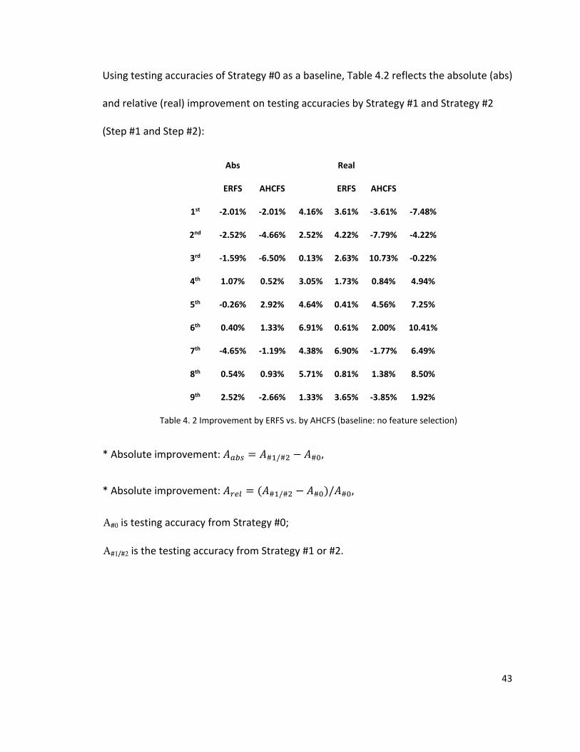
Using testing accuracies of Strategy #0 as a baseline, Table 4.2 reflects the absolute (abs)

and relative (real) improvement on testing accuracies by Strategy #1 and Strategy #2

(Step #1 and Step #2):

Abs Real

ERFS AHCFS ERFS AHCFS

1st -2.01% -2.01% 4.16% 3.61% -3.61% -7.48%

2nd -2.52% -4.66% 2.52% 4.22% -7.79% -4.22%

3rd -1.59% -6.50% 0.13% 2.63% 10.73% -0.22%

4th 1.07% 0.52% 3.05% 1.73% 0.84% 4.94%

5th -0.26% 2.92% 4.64% 0.41% 4.56% 7.25%

6th 0.40% 1.33% 6.91% 0.61% 2.00% 10.41%

7th -4.65% -1.19% 4.38% 6.90% -1.77% 6.49%

8th 0.54% 0.93% 5.71% 0.81% 1.38% 8.50%

9th 2.52% -2.66% 1.33% 3.65% -3.85% 1.92%

Table 4. 2 Improvement by ERFS vs. by AHCFS (baseline: no feature selection)

* Absolute improvement: 𝑆𝑆𝑡𝑡𝑎𝑎𝑦𝑦 = 𝑆𝑆#1/#2 − 𝑆𝑆#0,

* Absolute improvement: 𝑆𝑆𝑦𝑦𝑦𝑦𝑙𝑙 = (𝑆𝑆#1/#2 − 𝑆𝑆#0)/𝑆𝑆#0,

A#0 is testing accuracy from Strategy #0;

A#1/#2 is the testing accuracy from Strategy #1 or #2.

44

Strategy #1 sometimes fails to improve testing accuracies. The rate of effectively

improved cases is 31.8%, the highest improved accuracy is 2.52% (abs) & 3.65% (rel).

Without FS vs. AHCFS

Compare to Strategy #0 (Without FS), Strategy #2 (AHCFS) works much better. Strategy

#2 outperforms 6 out of 9 weekly average. However, it still doesn't work out for small

step sizes. The rate of effectively improved cases is 70.5%, and most cases are improved

by using Strategy #2. The highest improved accuracy is 6.91% (abs) and 10.41% (rel).

ERFS vs. AHCFS Step #1 & Step #2

As two similar algorithms, we would like to see if Strategy #2 Step #1 works better than

Strategy #1. The answer is positive. Based on Strategy #0’s results, Strategy #2 Step #1’s

rate of effective cases is 38.6%, which is higher than Strategy #1’s, at 31.8%.

Compared to Strategy #2 Step #2 (Strategy #2 Step #2 equals Strategy #2), the rates of

effectively improved cases, using Strategy #0's results as a basis, are 31.8% vs. 70.5%.

Numbers of improved weekly averages are 4/9 versus 6/9. The highest improvement is

2.52% versus 6.91% (abs). Strategy #2 Step #2 is significantly better.

Without FS vs. ERFS

Compared to Strategy #0 (Without FS), Strategy #1 (ERFS) is not very stable or effective.

in 1st,2nd, 3rd, 5th,6th, 5 out of 9 weekly average, Strategy #1 underperforms Strategy #0.

For small step sizes (<21 days), Strategy #1 does not work better, and for large step size,

45

4.3 Scenario 2: Experiment based on data with sharp changes (2000–2010)










d. Date: IS = 2000 – 2007; OOS = 2007 – 2010





Figure 4.2 presents the trending of the S&P500 from 2000 to 2010, and Table 4.3

presents the testing (OOS) accuracies based on the above piece of data (data period

2000–2012). Compared to 2007-2017, 2000-2010 includes some similarities and some

significant differences. The training part is similar in some respects: it begins with a

downslope that lasts three years, and then shows a more gradual increase until the

separation line. The testing part shows a sharp decrease - a significant drop due to the

46

subprime mortgage crisis, and then it picks up a little bit just after a crisis. It is a

relatively difficult prediction since the testing (unknown) data begins with a big change

in direction, which is inconsistent with training data. However, with the small rebound

after 2009, the testing data looks like the training data in miniature. However, the

trading volume during the drop (2009) in 2007-2017 fluctuates significantly while the

trading volume during the drop (2003) in 2000-2010 fluctuates very slightly.


In general, Strategy #0 is ineffective. The testing accuracies vary from 49.51% to 55.37%,

which is as ineffective as a guess with just 50% accuracy. The standard deviation is equal

to or less than 2%, except for the 1st week, which means the fluctuation in testing

accuracies is relatively small. The testing accuracies of Strategy #1 range from 49.16% to

72.39%, except during the 9th week's 78.75% (a sudden high). The testing accuracies of

Strategy #2 range from 50.47% to 77.02%. Both Strategy #1 and #2 are within the

0

2E+09

4E+09

6E+09

8E+09

1E+10

1.2E+10

1.4E+10

0

200

400

600

800

1000

1200

1400

1600

1800

1/3/2000 1/3/2001 1/3/2002 1/3/2003 1/3/2004 1/3/2005 1/3/2006 1/3/2007 1/3/2008 1/3/2009 1/3/2010

2000-2010 S&P500 ^GSPC

Close Price Trading Volume

47

standard deviation at around 4% (#1 – 3.64%, #2 – 3.98%), which shows a more

substantial fluctuation in testing accuracies than Strategy #0.

Step Size accuracy% # of selected features 44 features

Without FS ERFS AHCFS ERFS AHCFS Step #1 Step #2 Step #1 Step #2

1st week Mean 49.51% 49.16% 50.66% 52.31% 6 5 7 SD 3.80% 3.47% 1.35% 3.55% 4.06 5.50 7.23 2nd week Mean 52.86% 50.08% 52.06% 50.47% 3 3 6 SD 1.89% 5.00% 2.71% 2.70% 0.50 2.06 3.96 3rd week Mean 54.31% 56.71% 57.64% 60.43% 12 6 10 SD 2.16% 2.97% 5.96% 5.34% 15.08 3.64 4.71 4th week Mean 55.37% 60.97% 60.70% 66.39% 6 13 19 SD 1.63% 4.61% 5.07% 6.63% 1.09 1.30 3.54 5th week Mean 53.51% 66.94% 70.12% 68.13% 22 12 15 SD 2.12% 2.19% 2.83% 1.06% 10.16 1.48 3.27 6th week Mean 51.39% 65.47% 68.93% 71.06% 6 9 14 SD 0.82% 3.06% 4.03% 5.35% 1.87 2.69 2.86 7th week Mean 50.00% 69.89% 70.96% 73.74% 7 8 14 SD 0.84% 3.90% 1.93% 3.22% 1.09 1.66 0.83 8th week Mean 49.93% 72.39% 67.21% 69.86% 8 12 16 SD 1.25% 3.79% 4.25% 2.52% 3.08 2.12 1.41 9th week Mean 50.07% 78.75% 73.84% 77.02% 7 12 13 SD 2.26% 3.80% 4.37% 5.45% 1.66 3.20 2.28


48

Using the testing accuracies of Strategy #0, Table 4.4 depicts the absolute and relative

improvement on testing accuracies by Strategy #1 and Strategy #2 (Step #1 and Step

#2):

Abs

Real

ERFS AHCFS

ERFS AHCFS

1st -0.35% 1.15% 2.81% -0.70% 2.33% 5.67%

2nd -2.78% -0.80% -2.39% -5.27% -1.52% -4.52%

3rd 2.40% 3.32% 6.12% 4.42% 6.12% 11.27%

4th 5.59% 5.32% 11.01% 10.10% 9.61% 19.89%

5th 13.42% 16.61% 14.61% 25.08% 31.03% 27.31%

6th 14.07% 17.54% 19.67% 27.39% 34.13% 38.27%

7th 19.89% 20.96% 23.74% 39.79% 41.91% 47.49%

8th 22.45% 17.27% 19.92% 44.97% 34.59% 39.90%

9th 28.68% 23.77% 26.95% 57.29% 47.46% 53.82%




𝑆𝑆#0 is testing accuracy from Strategy #0;

𝑆𝑆#1/#2 is the testing accuracy from Strategy #1 or #2.

49

Without FS vs. ERFS

Compared to Strategy #0, Strategy #1 is relatively effective but slightly less stable. In 7

of 9 weekly averages, Strategy #1 outperforms Strategy #0. However, it still does not

work out for small step sizes and works better in Scenario 1 (only two weekly averages

underperform in this case compared to 3 weekly averages underperforming in Scenario

1). The rate of effectively improved cases is 95.5%, and the highest improved accuracy

is 28.68% (abs) & 57.29% (rel).


Compared to Strategy #0, Strategy #2 exhibits better performance in effectiveness, but

not instability. In 8 out of 9 weekly averages, Strategy #2 outperforms Strategy #0. The

rate of effectively improved cases is 84.1%, and the highest accuracy is 26.95% (abs) and

53.82% (rel).

ERFS vs. AHCFS Step #1 & #2

Compared with Strategy #1, Strategy #2 Step #1 outperforms 6 out of 9 weekly

averages. However, the rate of effectively improved cases, using Strategy #0's results as

the basis, is 84.1%, which is slightly lower than Strategy #1.

Strategy #2 Step #2 (Strategy #2 Step#2 equals to Strategy #2, only when we mention

Strategy #1 do we use Strategy #2 Step #2 instead of Strategy #2) outperforms Strategy

#1 in terms of rate of effectively improved cases (84.1% vs. 84.1%) and number of

improved weekly averages (8/9 vs. 7/9). However, the highest improvement of Strategy

#2 is smaller.

50

4.4 Scenario 3: Experiment based on older data (1992–2002)










d. Date: IS = 1992 – 1999; OOS = 1999 – 2002



b. Strategy #2 Step #1: IS’:OOS’: 2:5; IS’ = 1992 – 1994, OOS’ = 1994 – 1999


Figure 4.3 shows the trending of the S&P500 from 1992 to 2002, and Table 4.5 is the

testing (OOS) accuracies based on the above data (data period 1992-2002). The trend

both in the training and testing parts are quite different from those in Scenarios 1 and 2.

The training part consists of two pieces of trends – the first piece is a slow increase and

the second piece is speeded increase. The testing part also consists of two pieces of

trends – the first piece is a sharp increase which is consistent with another piece in the

51

training part and the second piece is a significant decrease. Overall, it is correct to say

that the pattern of training data is quite different from that of the testing data.


In general, Strategy #0 doesn't work well in this case either. Its testing accuracies vary

from 46.20% to 50.00%, which is roughly equal to guess. It is ineffective. The weekly

standard deviation is about 2%. Testing accuracies of Strategy #1 vary from 49.94% to

63.52%, which is significant compared with Strategy #0. Its weekly standard deviation is

about 4.5%. The testing accuracies of Strategy #2 vary from 49.68% to 75.16%, which is

better than Strategy #1. Its weekly standard deviation is about 2.5%.

0

500000000

1E+09

1.5E+09

2E+09

2.5E+09

0

200

400

600

800

1000

1200

1400

1600

1800

1/2/1992 1/2/1993 1/2/1994 1/2/1995 1/2/1996 1/2/1997 1/2/1998 1/2/1999 1/2/2000 1/2/2001 1/2/2002

1992-2002 S&P500 ^GSPC


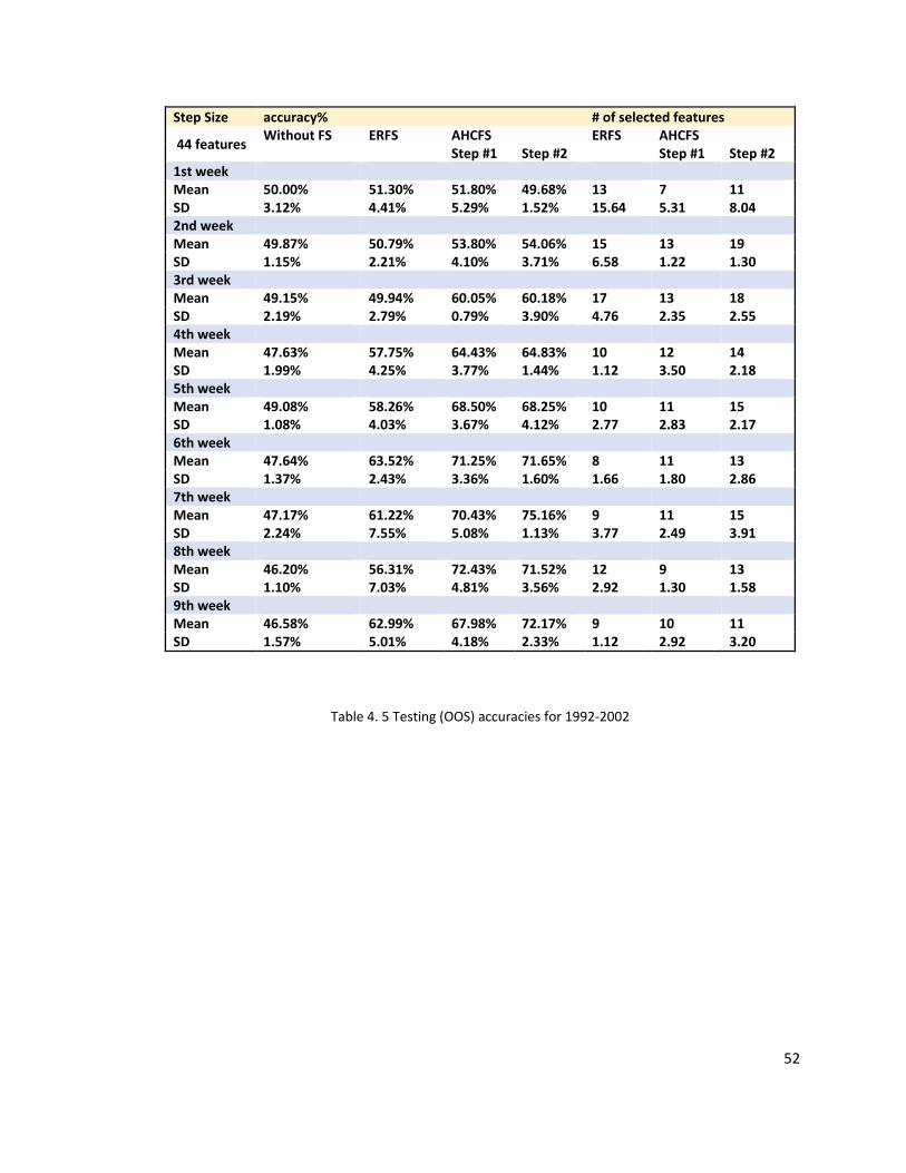
52

Step Size accuracy% # of selected features

44 features Without FS ERFS AHCFS ERFS AHCFS Step #1 Step #2 Step #1 Step #2

1st week Mean 50.00% 51.30% 51.80% 49.68% 13 7 11 SD 3.12% 4.41% 5.29% 1.52% 15.64 5.31 8.04 2nd week Mean 49.87% 50.79% 53.80% 54.06% 15 13 19 SD 1.15% 2.21% 4.10% 3.71% 6.58 1.22 1.30 3rd week Mean 49.15% 49.94% 60.05% 60.18% 17 13 18 SD 2.19% 2.79% 0.79% 3.90% 4.76 2.35 2.55 4th week Mean 47.63% 57.75% 64.43% 64.83% 10 12 14 SD 1.99% 4.25% 3.77% 1.44% 1.12 3.50 2.18 5th week Mean 49.08% 58.26% 68.50% 68.25% 10 11 15 SD 1.08% 4.03% 3.67% 4.12% 2.77 2.83 2.17 6th week Mean 47.64% 63.52% 71.25% 71.65% 8 11 13 SD 1.37% 2.43% 3.36% 1.60% 1.66 1.80 2.86 7th week Mean 47.17% 61.22% 70.43% 75.16% 9 11 15 SD 2.24% 7.55% 5.08% 1.13% 3.77 2.49 3.91 8th week Mean 46.20% 56.31% 72.43% 71.52% 12 9 13 SD 1.10% 7.03% 4.81% 3.56% 2.92 1.30 1.58 9th week Mean 46.58% 62.99% 67.98% 72.17% 9 10 11 SD 1.57% 5.01% 4.18% 2.33% 1.12 2.92 3.20


53



#2):

Abs

Real

ERFS AHCFS

ERFS AHCFS

1st 1.30% 1.80% -0.33% 2.60% 3.60% -0.66%

2nd 0.92% 3.93% 4.19% 1.84% 7.87% 8.40%

3rd 0.79% 10.91% 11.03% 1.60% 22.19% 22.44%

4th 10.12% 16.79% 17.19% 21.24% 35.26% 36.09%

5th 9.18% 19.41% 19.17% 18.71% 39.56% 39.05%

6th 15.88% 23.61% 24.01% 33.35% 49.57% 50.41%

7th 14.05% 23.26% 27.99% 29.78% 49.30% 59.33%

8th 10.11% 26.23% 25.32% 21.88% 56.78% 54.80%

9th 16.41% 21.39% 25.59% 35.22% 45.92% 54.93%




𝑆𝑆#0 is the testing accuracy from Strategy #0;

𝑆𝑆#1/#2 is the testing accuracy from Strategy #1 or #2.

54

Without FS vs. ERFS

In 9 out of 9 weekly averages, Strategy #1 outperforms Strategy #0, however, for small

step sizes (1st, 2nd, third weeks), the improvement is so insignificant (1.3%, 0.92%, 0.79%)

that it can be disregarded. The rate of effectively improved cases is 88.6%; the highest

testing accuracy improvement is 16.41% (abs) and 35.22% (rel).


In 8 out of 9 weekly averages, Strategy #2 outperforms Strategy #0. The 1st week is

below average insignificantly (-0.33%) as well. The 2nd week's improvement is slightly

insignificant (4.19%) as well. Still, they do not work well for the small step sizes. The rate

of effectively improved cases is 93.18%, and the highest improvement is 27.99% (abs)

and 59.33% (rel).

ERFS vs. AHCFS Step #1 & #2

Compared with Strategy #2 Step #1, Strategy #1 provides a lower rate of effective

improved cases (88.6% vs 90.9%), lower highest improvement (16.41% abs vs. 26.23%

abs), and larger weekly standard deviation (4.41% vs. 3.89%).

Compared with Strategy #2 Step #2, Strategy #1 provides a lower rate of effectively

improved cases (88.6% vs. 93.2%), lower highest improvement (16.41% abs vs. 27.99%

abs), and a more substantial weekly standard deviation (4.41% vs. 2.59%).

Both Strategy #2 Step #1 and #2 outperform Strategy #1 in this case.

55

4.5 Scenario 4: Experiment based on much older data (1960-1970)










d. Date: IS = 2000 – 2007; OOS = 2007 – 2010





Figure 4.4 demonstrates the trending of the S&P500 from 1960 to 1970, and Table 4.7

reflects the testing (OOS) accuracies based on the above data. The training part is an

increase in general with a sudden drop due to “Flash Crash” in 1962. The testing part

also generally increases with a sudden drop due to the 1967 “Sterling Crisis” and a weak

end.

56


In general, Strategy #0 works better than it does in the last case; its testing accuracies

vary from 53.58% to 60.03%. Its weekly standard deviation is about 1.5%. Strategy #1's

testing accuracies vary from 54.57% to 75.83%; its weekly standard deviation is about

4%. Strategy #2's testing accuracies vary from 54.56% to 82.45% (the highest). Its weekly

standard deviation is about 3.5%, which is lower than Strategy #1's.

0

5000000

10000000

15000000

20000000

25000000

0

20

40

60

80

100

120

1/4/1960 1/4/1961 1/4/1962 1/4/1963 1/4/1964 1/4/1965 1/4/1966 1/4/1967 1/4/1968 1/4/1969 1/4/1970

1960-1970 S&P500 ^GSPC


57

Step Size accuracy% # of selected features 44 features Without FS ERFS AHCFS ERFS AHCFS

Step #1 Step #2 Step #1 Step #2 1st week Mean 60.03% 60.70% 57.54% 54.56% 37 4 6 SD 1.23% 2.21% 5.12% 3.55% 7.84 3.67 3.77 2nd week Mean 58.30% 54.57% 56.98% 56.04% 25 4 7 SD 0.82% 7.16% 4.53% 4.62% 10.21 3.70 3.11 3rd week Mean 57.77% 57.37% 62.02% 61.36% 24 9 14 SD 1.18% 1.68% 2.50% 4.24% 15.12 3.00 5.41 4th week Mean 58.70% 62.95% 65.74% 75.04% 8 11 17 SD 1.40% 4.25% 4.73% 2.47% 0.87 3.35 2.55 5th week Mean 58.56% 66.93% 67.07% 74.24% 9 12 16 SD 1.16% 4.29% 5.64% 3.43% 3.77 2.50 5.12 6th week Mean 55.78% 69.45% 71.72% 79.81% 7 9 13 SD 0.90% 3.97% 2.90% 3.76% 2.28 1.66 1.58 7th week Mean 56.70% 75.83% 81.27% 81.27% 6 13 17 SD 1.46% 2.48% 3.21% 3.54% 1.09 2.29 2.69 8th week Mean 56.78% 74.34% 82.17% 82.45% 6 13 18 SD 1.78% 6.33% 3.22% 2.62% 1.48 1.87 1.22 9th week Mean 53.38% 74.37% 73.70% 79.94% 7 11 15 SD 1.91% 4.54% 3.51% 3.02% 3.96 2.95 4.09


58



#2):

Abs

Real

ERFS AHCFS

ERFS AHCFS

1st 0.66% -2.49% -5.47% 1.10% -4.15% -9.11%

2nd -3.73% -1.32% -2.26% -6.40% -2.27% -3.87%

3rd -0.40% 4.25% 3.59% -0.69% 7.36% 6.22%

4th 4.25% 7.05% 16.34% 7.25% 12.00% 27.84%

5th 8.37% 8.50% 15.68% 14.29% 14.52% 26.77%

6th 13.68% 15.94% 24.03% 24.52% 28.58% 43.09%

7th 19.13% 24.57% 24.57% 33.74% 43.33% 43.33%

8th 17.56% 25.40% 25.68% 30.93% 44.73% 45.22%

9th 20.99% 20.32% 26.56% 39.32% 38.06% 49.75%


Without FS vs. ERFS

In 7 out of 9 weekly averages, Strategy #1 outperforms Strategy #0, and the same

situation occurs. Although improvements appear in small step sizes, the improvements

are not significant. The rate of effectively improved cases is 75%, and the highest testing

accuracy improvement is 20.99% (abs) and 39.32% (rel).


In 7 out of 9 weekly averages, Strategy #2 outperforms Strategy #0; its performance

becomes better when step size becomes more substantial. The rate of effectively

59

improved cases is 81.8%, and the highest testing accuracy improvement is 26.56% (abs)

and 49.75% (rel).

ERFS vs. AHCFS Step #1 & Step #2

Compared with Strategy #2 Step #1, Strategy #1 gives a lower rate of effective improved

cases (75% vs. 86.3%) lower highest improvement (20.99% abs vs. 25.40% abs), and

larger weekly standard deviation (4.10% vs. 3.93%).

Compared with Strategy #2 Step #2, Strategy #1 gives a lower rate of effectively

improved cases (75% vs. 81.8%), lower highest improvement (20.99% abs vs. 26.56%

abs), and more substantial weekly standard deviation (4.10% vs. 3.47%).

Both Strategy #2 Step #1 and #2 outperform Strategy #1 in this case.

60

4.6 Others

One thing needs to be pointed out is that the SVM model without any feature selection

algorithm may not get well trained on a 10-year-long piece of data. That means the

results from Strategy #0 (Without FS) may suffer from an underfitting situation. The

extended experiment on the case of FS Strategy #0 (Without FS) suggests that the SVM

prediction model may need more data – a longer piece of data – to be sufficiently

trained to give stabilized predicting results, that somehow explains the significant

performance differences of Strategy #0 (Without FS) between in Scenario #1 and

Scenarios #2, 3, 4.

61

Chapter 5 Conclusion and Future Work

This work compared 3 SVM based strategies (algorithms) – #0: no FS, #1 ERFS, and #2

AHCFS on predicting market trends (up or down) of the S&P 500. Input data consists of

44 features drawn from 24 technical indicators. Additionally, several data groups are

collected and experimented within four different periods during which closing price

trends and trading volume trends are dissimilar. The prediction horizon is an

independent variable ranging from 1 to 60.

When the prediction horizon is smaller than two weeks (< 14 days), the prediction

accuracy difference from the three strategies is not significant. They are just around

50%, and any of these strategies can outperform others. When the prediction horizon is

more significant than three weeks (> 21 days), our target strategy - #2 always

outperforms the other two strategies. When the prediction horizon is between 2 weeks

and three weeks (14 days to 21 days), there is 1 case out of every four that our target

(strategy #2) does not significantly outperform (prediction accuracy is like) the other

two strategies. (*Due to space constraints, there is no detailed predicting of the results

given above. Instead, the weekly averages are shown as a summary to reduce the size of

the results table. All the detailed predicting results are listed in Appendix A.)

As a conclusion, our target #2 strategy—a prediction accuracy based hill climbing

feature selection algorithm (AHCFS)—works significantly better when the prediction

horizon exceeds three weeks (21 days).

62

The average numbers of features selected by strategy #2 after a prediction horizon

larger than three weeks (21 days) are between 10 and 20 (except in scenario 1) and

have smaller fluctuation, meaning higher stability compared to strategies #0 and #1.

SVM as a favorite machine learning technique is not the only tool we can use. This

algorithm can be tested based on other supervised machine learning techniques to fit

them better. Moreover, the other non-technical indicators, like macroeconomic

indicators, are not tested in this work. The mix of different kind of indicators could a

possible way to improve the prediction model. Also, the parameters of indicators could

be further optimized to improve the prediction results.

63

References

[1] F. X. Diebold and K. Yilmaz, Financial and Macroeconomic Connectedness: A

Network Approach to Measurement and Monitoring, New York: Oxford

University Press, 2015.

[2] J. Chen, "The Story of Technical Analysis: From the Japanese Rice Markets to Dow

Theory to Automated Trading," in Essentials of Technical Analysis for Financial

Markets, Hoboken, New Jersey., Wiley & Sons, Inc., 2010, pp. 11-24.

[3] K. G. Richards, Sideways: Using the Power of Technical Analysis to Profit in

Uncertain Times, Toronto and New York: BPS Books, 2011.

[4] Investopedia, "Technical Analysis," INVESTOPEDIA, 05 05 2016. [Online].

Available: https://www.investopedia.com/exam-guide/series-7/portfolio-

management/technical-

analysis.asp?ad=dirN&qo=investopediaSiteSearch&qsrc=0&o=40186.

[5] T. N. Bulkowski, "Fundamental Analysis Summary," in Fundamental Analysis and

Position Trading, Hoboken, John Wiley & Sons, Inc., 2012, pp. 95-99.

[6] R. Rhea, The Dow Theory, www.snowballpublishing.com, 2013.

64

[7] S. Matasyan, "The Dow Theory in Technical Analysis," 2013. [Online]. Available:

http://www.ifcmarkets.com/en/forex-trading-books/dow-theory-pdf.

[8] J. V. Bergen, "Efficient Market Hypothesis: Is The Stock Market Efficient?,"

INVESTOPEDIA, 17 02 2004. [Online]. Available:

https://www.investopedia.com/articles/basics/04/022004.asp.

[9] E. F. Fama, "Random Walks in Stock Market Prices," 1995. [Online]. Available:

https://www.cfapubs.org/doi/pdf/10.2469/faj.v51.n1.1861.

[10] A. Plastun, "Behavioral Finance Market Hypotheses," Oxford Scholarship Online,

2017.

[11] M. Santos, "Adaptive Markets Hypothesis: An Evolutionary View About the

Relationship Between Environmental Factors and Market Structure," SSRN

Electronic Journal, 2015.

[12] P. Rodriguez and S. Rivero, "Using Machine Learning Algorithms To Find Patterns

in Stock Prices," SSRN Electronic Journal, 2006.

[13] R. Dash and P. Dash, "A Hybrid Stock Trading Framework Integrating Technical

Analysis with Machine Learning Techniques," The Journal of Finance and Data

Science, vol. 2, no. 1, pp. 42-57, 2016.

65

[14] Y. Shynkevich, T. Mcginnity, S. Coleman, Y. Li and A. Belatreche, "Forecasting

stock price directional movements using technical indicators: Investigating

window size effects on one-step-ahead forecasting," in 2014 IEEE Conference on

Computational Intelligence for Financial Engineering & Economics (CIFEr),

London, UK, 2014.

[15] S. Niaki and S. Hoseinzade, "Forecasting S&P 500 Index Using Artificial Neural

Networks and Design of Experiments," Journal of Industrial Engineering

International, vol. 9, no. 1, 2013.

[16] O. Sezer, A. Ozbayoglu and E. Dogdu, "An Artificial Neural Network-based Stock

Trading System Using Technical Analysis and Big Data Framework," in The Annual

ACM Southeast Conference ACMSE 2017, Kennesaw, Georgia, 2017.

[17] P. Kantavat and B. Kijsirikul, "Combining Technical Analysis and Support Vector

Machine For Stock Trading," in 2008 Eighth International Conference on Hybrid

Intelligent System, Barcelona, Spain, 2008.

[18] Y. Lin, H. Guo and J. Hu, "An SVM-based Approach For Stock Market Trend

Prediction," in The 2013 International Joint Conference on Neural Networks

(IJCNN), Dallas, 2013.

[19] S. B. Achelis, Technical analysis from A to Z, New York: McGraw-Hill, 2000.

66

[20] I. Guyon and A. Elisseeff, "An Introduction to Variable and Feature selection,"

Journal of Machine Learning Research, no. 3, pp. 1157-1182, 2003.

[21] L. Ladha and T. Deepa, "Feature Selection Methods and Algorithms,"

International Journal on Computer Science and Engineering (IJCSE), vol. 3, no. 5,

pp. 1787-1797, 2011.

[22] D. W. Aha and R. L. Bankert, "A Comparative Evaluation of Sequential Feature

Selection Algorithms," in Learning from Data - Lecture Notes in Statistics vol. 112,

New York, Springer, 1996, pp. 199-206.

[23] B. Boser, I. Guyon and V. Vapnik, "A Training Algorithm For Optimal Margin

Classifiers," in COLT92 5th Annual Workshop on Computational Learning Theory,

New York, 1992.

[24] V. N. Vapnik, Statistical Learning Theory, John Wiley & Sons, INC., 1998.

[25] I. Steinwart and A. Christmann, "Introduction," in Support Vector Machine

(Information Science and Statistics), New York, Springer, 2008, pp. 01-19.

[26] T. Hastie, R. Tibshirani and J. Friedman, "Overview of Supervised Learning," in

Elements of Statistical Learning 1st edition, New York, Springer, 2016, pp. 9-39.

67

[27] N. Cristianini and J. Shawe-Taylor, An Introduction to Support Vector Machines

and Other Kernel-based Learning Methods, Cambridge: Cambridge University

Press, 2000.

[28] E. S. Youn, "Feature Selection In Support Vector Machines," 2002.

[29] S. Grigalunas, "List of Technical Indicators," Trading Technologies, 15 10 2015.

[Online]. Available: https://www.tradingtechnologies.com/help/x-

study/technical-indicator-definitions/list-of-technical-indicators/.

[30] StockCharts, "Technical Indicators and Overlays," StockCharts.com, 09 10 2017.

[Online]. Available:

http://stockcharts.com/school/doku.php?id=chart_school%3Atechnical_indicato

rs .

[31] A. T. Alali, "Application of Support Vector Machine in Predicting the Market’s

Monthly Trend Direction," 2013.

[32] S. Abe, "Feature Selection and Extraction," in Support Vector Machines for

Pattern Classification (Advances in Computer Vision and Pattern Recognition) 1st

edition, Springer, 2005, pp. 189-199.

68

Appendix A Summary Data Sheets

*Due to the size of data, detailed data can only be presented in digital format.

2007-2017

Step Size(days)

Without FS Simple Improved

44 features

accuracy%

Step #1 Step #2 # of selected features

# of selected features


1 47.02% 54.30% 58.94% 49.01% 2 1 2 2 59.33% 52.67% 54.00% 52.00% 11 2 7 3 57.33% 51.33% 50.67% 50.67% 10 2 2 4 58.94% 56.29% 50.99% 54.30% 4 3 5 Mean 55.66% 53.65% 53.65% 51.49% 7 2 4 Stddev 5.0425% 1.8533% 3.3192% 1.9382% 3.83 0.71 2.12 7 56.29% 54.97% 54.97% 54.97% 1 8 8 8 58.94% 52.32% 57.62% 55.63% 3 13 17 9 60.67% 59.33% 54.00% 57.33% 34 1 2 10 61.33% 60.00% 53.33% 62.67% 40 15 25 11 61.59% 59.60% 55.63% 55.63% 19 1 1 Mean 59.76% 57.24% 55.11% 57.25% 24 8 11 Stddev 1.9671% 3.0652% 1.4804% 2.8218% 14.34 6.54 10.16 14 62.25% 57.62% 49.01% 45.03% 7 10 14 15 61.59% 58.28% 56.95% 54.97% 25 12 15 16 62.00% 60.67% 54.00% 63.33% 13 1 7 17 58.28% 60.26% 54.30% 66.23% 30 14 35 18 58.94% 58.28% 56.29% 72.85% 21 9 21 Mean 60.61% 59.02% 54.11% 60.48% 22 9 20 Stddev 1.6620% 1.2111% 2.7907% 9.6240% 6.22 4.95 10.23 21 63.58% 63.58% 58.94% 58.94% 44 3 6 22 60.00% 59.33% 55.33% 58.67% 6 1 4 23 65.33% 71.33% 60.67% 67.33% 15 7 15 24 60.93% 58.94% 66.89% 68.21% 9 12 27 25 58.28% 60.26% 68.87% 70.20% 7 15 16 Mean 61.62% 62.69% 62.14% 64.67% 9 9 16 Stddev 2.5254% 4.6195% 5.0324% 4.8800% 3.49 5.31 8.14 28 63.58% 62.25% 69.54% 66.89% 14 15 23 29 60.67% 60.67% 60.00% 61.33% 33 14 18 30 66.67% 66.67% 69.33% 70.67% 22 12 12 31 66.23% 64.24% 68.21% 72.19% 6 10 19 32 62.91% 64.90% 67.55% 72.19% 28 13 12

69

Mean 64.01% 63.74% 66.93% 68.65% 22 12 15 Stddev 2.2151% 2.0891% 3.5390% 4.1402% 10.16 1.48 3.27 35 64.90% 59.60% 71.52% 72.19% 5 12 20 36 66.00% 66.67% 60.67% 72.67% 7 15 21 37 66.67% 71.33% 73.33% 78.00% 7 15 21 38 68.21% 68.21% 63.58% 73.51% 39 14 20 39 66.23% 68.21% 69.54% 70.20% 35 15 19 Mean 66.40% 66.81% 67.73% 73.31% 22 15 20 Stddev 1.0764% 3.9079% 4.8207% 2.5844% 15.07 0.43 0.83 42 68.87% 61.59% 68.21% 72.85% 6 4 9 43 65.33% 53.33% 64.00% 68.67% 6 8 19 44 66.67% 64.67% 68.67% 70.00% 5 14 29 45 67.55% 64.24% 63.58% 75.50% 27 12 23 46 68.87% 70.20% 66.89% 72.19% 35 5 15 Mean 67.46% 62.81% 66.27% 71.84% 18 10 22 Stddev 1.3535% 5.5023% 2.1122% 2.3648% 13.06 3.49 5.17 49 66.00% 72.67% 66.67% 66.67% 7 11 19 50 66.00% 68.67% 66.67% 76.00% 7 15 45 51 68.21% 67.55% 61.59% 70.86% 7 9 21 52 68.87% 64.90% 74.83% 77.48% 9 15 22 53 66.89% 64.90% 70.86% 73.51% 8 13 15 Mean 67.19% 67.74% 68.12% 72.90% 8 13 26 Stddev 1.1666% 2.8737% 4.4603% 3.8471% 0.83 2.45 11.43 56 70.00% 66.67% 64.00% 64.67% 3 8 15 57 66.00% 70.67% 67.33% 72.67% 5 10 13 58 69.54% 78.81% 70.20% 78.15% 10 10 12 59 70.20% 74.17% 60.93% 58.28% 4 1 2 60 69.54% 67.55% 69.54% 78.15% 4 12 16 Mean 69.05% 71.57% 66.40% 70.38% 6 8 11 Stddev 1.5490% 4.4762% 3.4886% 7.8095% 2.49 4.26 5.26

70

2000-2010

Step Size(days)


44 features

accuracy%




1 48.34% 54.30% 52.98% 56.29% 2 1 2 2 47.02% 49.67% 49.67% 54.97% 2 2 3 3 56.00% 44.67% 50.00% 47.33% 9 1 2 4 46.67% 48.00% 50.00% 50.67% 11 14 19 Mean 49.51% 49.16% 50.66% 52.31% 6 5 7 Stddev 3.8001% 3.4735% 1.3450% 3.5489% 4.06 5.50 7.23 7 52.98% 50.99% 53.64% 50.33% 5 1 4 8 50.33% 51.66% 47.02% 49.01% 2 1 3 9 51.66% 40.40% 54.97% 46.36% 3 6 13 10 56.00% 52.67% 52.67% 54.00% 2 2 4 11 53.33% 54.67% 52.00% 52.67% 3 1 5 Mean 52.86% 50.08% 52.06% 50.47% 3 3 6 Stddev 1.8944% 4.9960% 2.7103% 2.6966% 0.50 2.06 3.96 14 52.32% 51.66% 51.66% 54.97% 1 1 2 15 56.95% 56.95% 56.95% 53.64% 1 1 2 16 52.67% 60.67% 50.67% 61.33% 4 3 13 17 52.67% 56.00% 64.67% 65.33% 5 8 10 18 56.95% 58.28% 64.24% 66.89% 38 10 14 Mean 54.31% 56.71% 57.64% 60.43% 12 6 10 Stddev 2.1609% 2.9740% 5.9636% 5.3381% 15.08 3.64 4.71 21 57.62% 52.98% 52.98% 70.86% 1 1 15 22 56.29% 62.91% 60.26% 69.54% 4 11 13 23 55.33% 66.00% 67.33% 70.67% 7 14 20 24 52.67% 64.00% 58.00% 53.33% 6 14 22 25 54.97% 58.94% 64.90% 67.55% 6 14 21 Mean 55.37% 60.97% 60.70% 66.39% 6 13 19 Stddev 1.6349% 4.6091% 5.0739% 6.6333% 1.09 1.30 3.54 28 54.97% 64.90% 70.86% 66.23% 9 13 18 29 54.30% 64.24% 66.89% 68.21% 7 8 21 30 49.33% 66.67% 74.67% 68.00% 7 13 18 31 54.00% 69.33% 67.33% 69.33% 4 10 14 32 54.97% 69.54% 70.86% 68.87% 5 9 12 Mean 53.51% 66.94% 70.12% 68.13% 6 10 16 Stddev 2.1242% 2.1910% 2.8279% 1.0634% 1.30 1.87 3.49 35 51.66% 61.59% 70.20% 74.83% 4 7 18 36 52.32% 70.20% 66.23% 64.90% 8 7 12

71

37 50.00% 63.33% 74.67% 76.67% 7 8 16 38 52.00% 64.67% 70.67% 74.67% 6 6 10 39 50.99% 67.55% 62.91% 64.24% 3 13 17 Mean 51.39% 65.47% 68.93% 71.06% 6 9 14 Stddev 0.8238% 3.0645% 4.0260% 5.3509% 1.87 2.69 2.86 42 49.67% 70.20% 70.86% 70.20% 5 7 12 43 50.99% 72.85% 73.51% 69.54% 5 8 14 44 49.33% 69.33% 71.33% 75.33% 7 10 13 45 49.01% 62.91% 67.55% 76.82% 8 6 13 46 50.99% 74.17% 71.52% 76.82% 7 6 15 Mean 50.00% 69.89% 70.96% 73.74% 7 8 14 Stddev 0.8384% 3.9027% 1.9287% 3.2167% 1.09 1.66 0.83 49 49.01% 72.19% 64.24% 70.86% 6 8 16 50 49.33% 76.00% 70.00% 70.67% 13 9 14 51 50.00% 76.67% 70.67% 72.00% 6 11 16 52 49.01% 70.86% 60.26% 64.90% 8 14 18 53 52.32% 66.23% 70.86% 70.86% 5 14 16 Mean 49.93% 72.39% 67.21% 69.86% 8 12 16 Stddev 1.2464% 3.7870% 4.2456% 2.5231% 3.08 2.12 1.41 56 46.36% 72.19% 78.81% 81.46% 6 6 13 57 53.33% 81.33% 78.00% 80.00% 8 10 13 58 50.00% 78.00% 68.00% 68.00% 8 15 17 59 50.99% 83.44% 69.54% 73.51% 6 14 11 60 49.67% 78.81% 74.83% 82.12% 4 7 12 Mean 50.07% 78.75% 73.84% 77.02% 7 12 13 Stddev 2.2561% 3.8043% 4.3727% 5.4452% 1.66 3.20 2.28

72

1992-2002

Step Size(days)


44 features

accuracy%





73


74

1960-1970

Step Size(days)

Without FS

Simple Improved

44 features

accuracy%

Step #1 Step #2 # of

selected features




75


76

Appendix B Maltab Codes

SVM based prediction with AHCFS as a feature selection method

clear

close all

format compact

addpath '..\misc2'

addpath '..\ta-lib-0.0.3_ml2007a-mex_w64'

% Pre-allocat memory for saving intermediate and final results

resultsexcel = cell(65,13);

% Count running time

tstart = tic;

% Read raw data (original data from market)

[op, hi, lo, cl, vo, dt, dn, ds, d] = read_data('SP500_GSPC_D.csv');

%%%%%%%%%%%%%%%%%%%%%%%%%%%%%%%%%%%%%%%%%%%%%%%%%%%%%%%%%%%%%%%%%%%%%%%

%%%%

% Test effect of improved feature selection algorithm on a

changeable ...

% step size basis

% for nn = 58 % Step size/Prediction horizon (including

alternatives)

for nn = [56:60]

% for nn = [28:32, 35:39, 42:46, 49:53]

77

% for nn = [1:4, 7:11, 14:18, 21:25, 28:32, 35:39, 42:46, 49:53, 56:60]

disp('****************')

nn

% Pre-process data for technical indicator calculations

[thui, frii] = find_indicies(nn, dt, dn);

thfi = [thui, frii, (frii - thui)];

NumDays = daysAct_RPT(dn(thui), dn(frii));

[~,DAYNAME] = weekday(dn(thui));

% stk.d = d;

% stk.d = d(thui);

% stk.o = op;

% stk.h = hi;

% stk.l = lo;

% stk.c = cl;

% stk.c = cl(thui);

% stk.c_F = cl(frii);

% stk.v = vo;

stk.d = d(thui);

stk.o = op(thui);

stk.h = hi(thui);

stk.l = lo(thui);

stk.c = cl(thui);

stk.c_F = cl(frii);

stk.v = vo(thui);

stk.oh = TA_MAX(stk.c,12);

78

stk.ol = TA_MIN(stk.c,12);

%%%%%%%%%%%%%%%%%%%%%%%%%%%%%%%%%%%%%%%%%%%%%%%%%%%%%%%%%%%%%%%%%%%%%%%

%%%%

% Calculate technical indicators, further create feature set and

% training target set as SVM inputs

features_store = technical_indicators(stk);

features_store(isnan(features_store)) = 0;

features = features_store;

features_copy = features;

CorrectTargets = stk.c_F >= stk.c;

%%%%%%%%%%%%%%%%%%%%%%%%%%%%%%%%%%%%%%%%%%%%%%%%%%%%%%%%%%%%%%%%%%%%%%%

%%%%

% Create time label to partition data for training and testing aims

T1 = find(stk.d >= 20020101, 1); % T1 - T2: IS' for filter method

T2 = find(stk.d >= 20040101, 1); % T2 - T3: OOS' for fitler method

T3 = find(stk.d >= 20090101, 1); % T1 - T3: IS for SVM training

T4 = find(stk.d >= 20120101, 1); % T3 - T4: OOS for SVM testing

IS_Set_FS = features(T1:T2-1,:);

IS_CorrectTargets_FS = CorrectTargets(T1:T2-1);

OOS_Set_FS = features(T2:T3-1,:);

OOS_CorrectTargets_FS = CorrectTargets(T2:T3-1);

79

%%%%%%%%%%%%%%%%%%%%%%%%%%%%%%%%%%%%%%%%%%%%%%%%%%%%%%%%%%%%%%%%%%%%%%%

%%%%

% Apply feature selection algorithms

[l, fn] =

sequential_QILI_2(IS_Set_FS,IS_CorrectTargets_FS,OOS_Set_FS,OOS_Correct

Targets_FS);

[~,fn_qi,lp] =

imp_seq_1(l,fn,nn,IS_Set_FS,IS_CorrectTargets_FS,OOS_Set_FS,OOS_Correct

Targets_FS);

%%%%%%%%%%%%%%%%%%%%%%%%%%%%%%%%%%%%%%%%%%%%%%%%%%%%%%%%%%%%%%%%%%%%%%%

%%%%

IS_CorrectTargets = CorrectTargets(T1:T3-1); %T1 - T3

OOS_CorrectTargets = CorrectTargets(T3:T4);

l =

get_results_seq(fn,features_copy,T1,T3,T4,IS_CorrectTargets,OOS_Correct

Targets); %T1 - T3

l_qi =

get_results_imp_seq(fn_qi,features_copy,T1,T3,T4,IS_CorrectTargets,OOS_

CorrectTargets); %T1 - T3

resultsexcel =

store_results_others(resultsexcel,nn,IS_CorrectTargets,OOS_CorrectTarge

ts);

resultsexcel = store_results_seq(resultsexcel,nn,l,fn);

80

resultsexcel = store_results_imp_seq(resultsexcel,nn,fn_qi,l_qi);

end

telapsed = toc(tstart)

telapsed_min = telapsed/60

telapsed_hr = telapsed_min/60

resultsexcel = write_to_excel(resultsexcel);

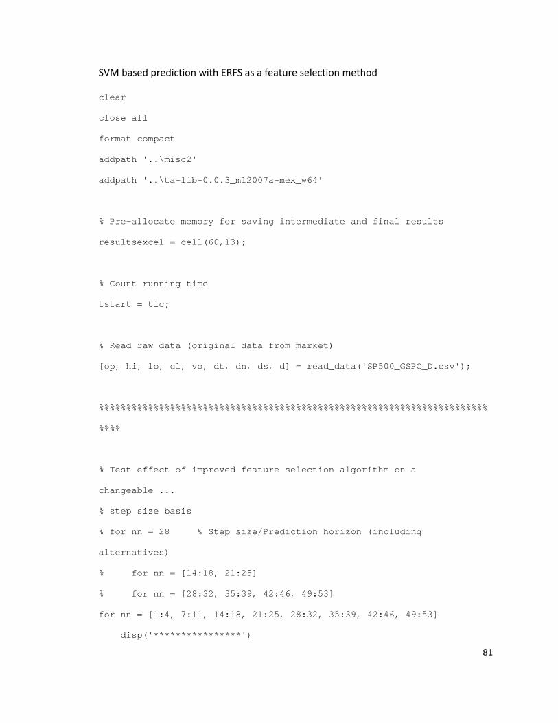
81

SVM based prediction with ERFS as a feature selection method

clear

close all

format compact

addpath '..\misc2'


% Pre-allocate memory for saving intermediate and final results

resultsexcel = cell(60,13);

% Count running time

tstart = tic;

% Read raw data (original data from market)


%%%%%%%%%%%%%%%%%%%%%%%%%%%%%%%%%%%%%%%%%%%%%%%%%%%%%%%%%%%%%%%%%%%%%%%

%%%%

% Test effect of improved feature selection algorithm on a

changeable ...

% step size basis

% for nn = 28 % Step size/Prediction horizon (including

alternatives)

% for nn = [14:18, 21:25]

% for nn = [28:32, 35:39, 42:46, 49:53]

for nn = [1:4, 7:11, 14:18, 21:25, 28:32, 35:39, 42:46, 49:53]

disp('****************')

82

nn

% Pre-process data for technical indicator calculations





% stk.d = d;

% stk.d = d(thui);

% stk.o = op;

% stk.h = hi;

% stk.l = lo;

% stk.c = cl;

% stk.c = cl(thui);


% stk.v = vo;

stk.d = d(thui);

stk.o = op(thui);

stk.h = hi(thui);

stk.l = lo(thui);

stk.c = cl(thui);

stk.c_F = cl(frii);

stk.v = vo(thui);



83

%%%%%%%%%%%%%%%%%%%%%%%%%%%%%%%%%%%%%%%%%%%%%%%%%%%%%%%%%%%%%%%%%%%%%%%

%%%%

% Calculate technical indicators, further create feature set and

% training target set as SVM inputs




features_copy = features;


%%%%%%%%%%%%%%%%%%%%%%%%%%%%%%%%%%%%%%%%%%%%%%%%%%%%%%%%%%%%%%%%%%%%%%%

%%%%

% Create time label to partition data for training and testing aims

T1 = find(stk.d >= 20030101, 1); % T1 - T2: IS' for filter method

T2 = find(stk.d >= 20100101, 1); % T2 - T3: OOS' for filter method

T3 = find(stk.d >= 20130101, 1); % T1 - T3: IS for SVM training

T4 = find(stk.d >= 20170101, 1); % T3 - T4: OOS for SVM testing

IS_Set_FS = features(T1:T2-1,:);

IS_CorrectTargets_FS = CorrectTargets(T1:T2-1);

OOS_Set_FS = features(T2:T3-1,:);

OOS_CorrectTargets_FS = CorrectTargets(T2:T3-1);

IS_Set_SFS = features(T1:T3-1,:);

OOS_Set = features(T3:T4,:);

IS_CorrectTargets_SFS = CorrectTargets(T1:T3-1);

84


%%%%%%%%%%%%%%%%%%%%%%%%%%%%%%%%%%%%%%%%%%%%%%%%%%%%%%%%%%%%%%%%%%%%%%%

%%%%

% Sequential FS on an error rate filter basis

z = size(features,2);

maxdev = 0.001;

opt = statset('display','iter','TolFun',maxdev,'TolTypeFun','abs');

[inmodel,history] =

sequentialfs(@cfun,IS_Set_SFS,IS_CorrectTargets_SFS,...

'cv','none',...

'options',opt,...

'NFeatures', z,...

'direction','forward');

% Test prediction accuracies of all feature combination on testing

data

IS_Set = features(T1:T3-1,:);


IS_CorrectTargets = CorrectTargets(T1:T3-1);


accuracy = zeros(size(features,2),1);

for n = 1:size(features,2)

accuracy(n) =

OOS_precision(IS_Set_FS(:,history.In(n,:)),IS_CorrectTargets_FS,OOS_Set

_FS(:,history.In(n,:)),OOS_CorrectTargets_FS);

end

[acc,ind] = max(accuracy);

85

feats = find(history.In(ind,:));

acc_OOS =

OOS_precision(IS_Set(:,feats),IS_CorrectTargets,OOS_Set(:,feats),OOS_Co

rrectTargets);

resultsexcel{nn+2,1} = nn;

resultsexcel{nn+2,2} = acc_OOS;

resultsexcel{nn+2,3} = num2str(feats);

%%%%%%%%%%%%%%%%%%%%%%%%%%%%%%%%%%%%%%%%%%%%%%%%%%%%%%%%%%%%%%%%%%%%%%%

%%%%

% resultsexcel =

store_results_others(resultsexcel,nn,m,IS_CorrectTargets,OOS_CorrectTar

gets);

% resultsexcel = store_results_seq(resultsexcel,nn,l,fn);

% resultsexcel = store_results_imp_seq(resultsexcel,nn,fn_qi,l_qi);

end




resultsexcel = write_to_excel(resultsexcel);

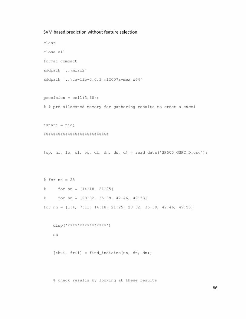
86

SVM based prediction without feature selection

clear

close all

format compact

addpath '..\misc2'


precision = cell(3,60);

% % pre-allocated memory for gathering results to creat a excel

tstart = tic;

%%%%%%%%%%%%%%%%%%%%%%%%%%%


% for nn = 28

% for nn = [14:18, 21:25]

% for nn = [28:32, 35:39, 42:46, 49:53]

for nn = [1:4, 7:11, 14:18, 21:25, 28:32, 35:39, 42:46, 49:53]

disp('****************')

nn


% check results by looking at these results

87




%%%%%%%%%%%%%%%%%%%%%%%%%%%%%%%%

%

% stk.d = d;

% stk.d = d(thui);

% stk.o = op;

% stk.h = hi;

% stk.l = lo;

% stk.c = cl;

% stk.c = cl(thui);


% stk.v = vo;

%

stk.d = d(thui);

stk.o = op(thui);

stk.h = hi(thui);

stk.l = lo(thui);

stk.c = cl(thui);

stk.c_F = cl(frii);

stk.v = vo(thui);



%%%%%%%%%%%%%%%%%%%%%%%%%%%%%%%%

88




%%%%%%%%%%%%%%%%%%%%%%%%%%%%%%%%%%%%%%%%%%%%%%%%


T1 = find(stk.d >= 20020101, 1);

T2 = find(stk.d >= 20090101, 1);

T3 = find(stk.d >= 20120101, 1);



IS_CorrectTargets = CorrectTargets(T1:T2-1);


precision{2,nn} =

OOS_precision(IS_Set,IS_CorrectTargets,OOS_Set,OOS_CorrectTargets);

resultsexcel{nn+2,1} = nn;

resultsexcel{nn+2,2} = precision{2,nn};

end


89



resultsexcel = write_to_excel_withoutFS(resultsexcel);

90

Sub Functions

cfun.m

function errRate = cfun(X,Y)

svmStruct = svmtrain(X, Y, 'kernel_function', 'rbf');

YY = svmclassify(svmStruct,X);

errRate = sum(YY ~= Y)/length(Y); % mis-classification rate

daysAct_RPT.m

function NumDays = daysAct( StartDate, EndDate )

%daysact Actual number of days between dates

% Given two dates in serial date numbers or date strings, calculate

the

% actual number of days between them

%

% NumDays = daysact(StartDate, EndDate)

%

% Inputs:

% StartDate (required) - The starting date in serial date number or

date

% string format

% EndDate (optional) - The ending date in serial date number or date

% string format. Defaults to the MATLAB base date (1-Jan-0000 AD)

% Author(s): B. Blunk 02/11/05 [email protected]

91

if(nargin < 1)

error('You must specify StartDate')

end

if(nargin < 2)

EndDate = 0;

end

if ((size(StartDate,1) ~= 0) & (size(EndDate,1) ~=0) & (size(EndDate,1)

~= size(StartDate,1)))

error('StartDate and EndDate must be of same size or scalar')

end

NumDays = datenum(datevec(EndDate)) - datenum(datevec(StartDate));

find_indicies.m

function [thui, frii] = find_indicies(nn, dt, dn)

%UNTITLED5 Summary of this function goes here

% Detailed explanation goes here

frii = find(weekday(dt) == 6);

% find all Fridays

frii = frii(10:end);

% start with the third Friday

thui = [];

for k = frii

for n = 1:70

92

nd = daysAct_RPT(dn(k-n), dn(k));

% find the number of days between two dates

if nd >= nn

thui = [thui, (k-n)];

break

end

end

end

end

get_results_imp_seq.m

function l_qi =

get_results_imp_seq(fn_qi,features_copy,T1,T4,T5,IS_CorrectTargets,OOS_

CorrectTargets)

% QILI method accuracy

if ~fn_qi(1) == 0;

features = features_copy(:,fn_qi);



l_qi =

OOS_precision(IS_Set,IS_CorrectTargets,OOS_Set,OOS_CorrectTargets);

end

end

93

get_results_seq.m

function l =

get_results_seq(fn,features_copy,T1,T3,T4,IS_CorrectTargets,OOS_Correct

Targets)

% Sequential method accuracy

features = features_copy(:,fn);



l = OOS_precision(IS_Set,IS_CorrectTargets,OOS_Set,OOS_CorrectTargets);

end

imp_seq_1.m

function [acc_out,features_out,num_loops] =

imp_seq_1(acc_in,features_in,nn,IS_Set0,IS_CorrectTargets,OOS_Set0,OOS_

CorrectTargets)

features_out = features_in;

acc_out = acc_in;

for x = 1:3

key = 1;

num_loops = 1;

acc_test1 = 0;

acc_test2 = 0;

while key == 1

key1 = 1;

key2 = 1;

94

fprintf('%d - %d\n',nn,num_loops);

features_test1 = 0;

add = 0;

while 1

add = add + 1;

accuracyI = zeros(1,size(OOS_Set0,2));

for k = 1:size(OOS_Set0,2)

fna = [features_out, k];

accuracyI(k) =

OOS_precision(IS_Set0(:,fna),IS_CorrectTargets,OOS_Set0(:,fna),OOS_Corr

ectTargets);

end

[acc_1, index_1]= max(accuracyI);

if acc_1 >= acc_out

if acc_1 == acc_out & index_1 == features_test1

% index_1 features_new|feautes_test1

features_old

key1 = 0;

break;

else

features_test1 = index_1;

end

fprintf('improved\n');

features_out = [features_out, index_1];

acc_out = acc_1;

add

acc_1

95

index_1

features_out

else

if add < 2

key1 = 0;

end

fprintf('no improvement\n');

add

acc_1

index_1

features_out

break;

end

end

features_test2 = 0;

sub = 0;

while 1

sub = sub + 1;

if length(features_out) > 1

accuracyII = zeros(1,size(features_out,2));

for k = 1:size(features_out,2)

fnr = subtract_feature_n(features_out, k);

accuracyII(k) =

OOS_precision(IS_Set0(:,fnr),IS_CorrectTargets,OOS_Set0(:,fnr),OOS_Corr

ectTargets);

end

[acc_2, index_2] = max(accuracyII);

96

if acc_2 >= acc_out

if features_out(index_2) == features_test2

key1 = 0;

key2 = 0;

fprintf('repeated\n');

break;

end

features_test2 = features_out(index_2);

fprintf('improved\n');

features_out(index_2) = [];

acc_out = acc_2;

sub

acc_2

index_2

features_out

else

if sub < 2

key2 = 0;

end

fprintf('no improvement\n');

sub

acc_2

index_2

features_out

break;

end

else

97

key2 = 0;

fprintf('only one selected feature\n');

break;

end

end

if acc_out == acc_test1

acc_test2 = acc_test2 + 1;

end

acc_test1 = acc_out;

if (key1||key2) == 0||acc_test2 == 1

key = 0;

end

num_loops = num_loops + 1;

end

if x > 1

if acc_out <= acc_previous

break;

end

end

acc_previous = acc_out;

end

end

function features__1 = subtract_feature_n(features, n)

98

features(:,n) = [];

features__1 = features;

end

OOS_precision.m

function precision =

OOS_precision(IS_Set,IS_CorrectTargets,OOS_Set,OOS_CorrectTargets)

% svmStruct = svmtrain(IS_Set, IS_CorrectTargets,'autoscale',true, ...

% 'kernel_function','rbf','method','LS');

%

% YY = svmclassify(svmStruct,IS_Set);

% errRate = sum(YY ~= IS_CorrectTargets)/length(IS_CorrectTargets);

% fprintf('inmodel SVM Accuracy: %6.2f %%\n', 100-errRate*100); %

inmodel SVM Accuracy

[r, ~] = size(IS_Set);

XX = [IS_Set; OOS_Set];

YY = [IS_CorrectTargets; OOS_CorrectTargets];

a = 0;

for n=1:length(OOS_Set)

XXN = zscore(XX(1:r+n, :)); % choose the desired normalization

method

svmStruct = svmtrain(XXN(1:end-1, :), YY(1:r+n-1), ...

99

'kernel_function','rbf','autoscale',false,'method','LS','rbf_sigma',1,'

boxconstraint',1);

Results(n, 1) = svmclassify(svmStruct, XXN(end,:));

end

compare = (Results == OOS_CorrectTargets);

precision = (sum(compare)/length(compare)*100);

%conMat = confusionmat(OOS_CorrectTargets,Results); % the confusion

matrix

res = [Results, OOS_CorrectTargets];

%Display Results

%fprintf('Out-of-Sample Accuracy: %6.2f %%\n', precision);

% rankfIS = rankfeatures(IS_Set', IS_CorrectTargets);

% rankfOOS = rankfeatures(OOS_Set', OOS_CorrectTargets);

% rankf = [rankfIS rankfOOS]

%accuracy(z) = (precision);

end

read_data.m

function [op, hi, lo, cl, vo, dt, dn, ds, d] = read_data( filename )

%UNTITLED4 Summary of this function goes here


100

%fid = fopen('SP500_RPT.csv');

fid = fopen(filename);

% ^GSPC data from Yahoo

C = textscan(fid, '%s%f%f%f%f%f%f','Delimiter',',','Headerlines',1);

fclose(fid);

dt = C{1}(end:-1:1);

% format is 'yyyy-mm-dd', e.g. '2013-11-29' cell

formatIn = 'yyyy-mm-dd';

dn = datenum(dt,formatIn);

formatOut = 'yyyymmdd';

ds = datestr(dn,formatOut);

% change format to 'yyyymmdd' char array (string)

d = str2num(ds);

% change string to number

op = C{2}(end:-1:1);

hi = C{3}(end:-1:1);

lo = C{4}(end:-1:1);

%c = C{5}(end:-1:1);

cl = C{7}(end:-1:1);

vo = C{6}(end:-1:1);

end

101

sequential_QILI_2.m

function [acc_seq, feats] =

sequential_QILI(IS_Set0,IS_CorrectTargets,OOS_Set0,OOS_CorrectTargets)

z = 15;

[accuracy,his] =

seq_2(IS_Set0,IS_CorrectTargets,OOS_Set0,OOS_CorrectTargets,z);

[acc_seq, acc_seq_i] = max(accuracy);

% Check intermediate results

fprintf('First %d In-Sample Accuracies of feature combinations: \n',z);

accuracy

feats = find(his.a(acc_seq_i,:));

%Check intermediate results

fprintf('Best combination and In-Sample Accuracy: \n');

feats

acc_seq

end

store_results_imp.m

function [acc_seq, feats] =

sequential_QILI(IS_Set0,IS_CorrectTargets,OOS_Set0,OOS_CorrectTargets)

z = 15;

[accuracy,his] =

seq_2(IS_Set0,IS_CorrectTargets,OOS_Set0,OOS_CorrectTargets,z);

102

[acc_seq, acc_seq_i] = max(accuracy);

% Check intermediate results

fprintf('First %d In-Sample Accuracies of feature combinations: \n',z);

accuracy

feats = find(his.a(acc_seq_i,:));

%Check intermediate results

fprintf('Best combination and In-Sample Accuracy: \n');

feats

acc_seq

end

store_results_others.m

function [ resultsexcel ] =

store_results_others(resultsexcel,nn,IS_CorrectTargets,OOS_CorrectTarge

ts)

resultsexcel{nn+2,1} = nn; % get number of day

%%%%%%%%%%%%%%%%%%%%

len = length(OOS_CorrectTargets);

resultsexcel{nn+2,8} = sum(OOS_CorrectTargets)/len; % always UP

%%%%%%%%%%%%%%%%%%%%

targets = [IS_CorrectTargets(end);OOS_CorrectTargets];

resultsexcel{nn+2,9} = sum(diff(targets) == 0)/len; % same as previous

%%%%%%%%%%%%%%%%%%%%

103

resultsexcel{nn+2,10} = sum(diff(targets) ~= 0)/len;% different from

previous

%resultsexcel{nn+2,4} = m; %num2str(m); %m;

end

store_results_seq.m

function [ resultsexcel ] = store_results_seq(resultsexcel,nn,l,fn)

resultsexcel{nn+2,2} = l;

resultsexcel{nn+2,3} = num2str(fn);

end

technical_indicators.m

function [ indicators ] = technical_indicators(stk)

%UNTITLED Summary of this function goes here


% Calculate Technicals

I1 = TA_RSI(stk.c, 14);

[bBandsHigh, bBandsMid, bBandsLow] = TA_BBANDS(stk.c,9,2,2);

I2 = (stk.c - bBandsHigh)./bBandsHigh;

I3 = (stk.c - bBandsLow)./bBandsLow;

104

[stochK, stochD] = TA_STOCHF(stk.oh,stk.ol,stk.c, 14, 3);% 14,3

I4 = stochK;

I5 = stochD;

I6 = [nan; diff(stochK)];

I7 = [nan; diff(stochD)];

I8 = [nan; diff(stk.c)./stk.c(1:end-1)];

I9 = (stk.c - stk.ol)./(stk.h-stk.ol); % similar to StochRSI

PMAs = TA_SMA(stk.c,10);

PMAl = TA_SMA(stk.c,21);

I10 = [nan; diff(PMAs)./PMAs(1:end-1)];

I11 = [nan; diff(PMAl)./PMAl(1:end-1)];

I12 = [nan; (PMAs(2:end)-PMAl(1:end-1))./PMAl(1:end-1)];

I13 = (stk.c - PMAl)./PMAl;

I14 = (stk.c - TA_MIN(stk.c,5))./TA_MIN(stk.c,5);

I15 = (stk.c - TA_MAX(stk.c,5))./TA_MAX(stk.c,5);

I16 = (((TA_SMA(stk.c,5) - TA_SMA(stk.c,12)) ./ TA_SMA(stk.c,12))); %

MA

I17 = [nan(12,1); (stk.c(13:end) - stk.c(1:end-12)) ./ stk.c(1:end-

12)]; % MOM

I18 = TA_KAMA(stk.c,12); % Kaufman Adaptive Moving Average KAMA

I19 = ConnorsRSI(stk.c,6,3,85); % ConnorsRSI CRSI % 6,3,85 ->

64.18%

I20 = TA_MFI(stk.h,stk.l,stk.c,stk.v); % Money Flow Index MFI

I21 = TA_BOP(stk.o,stk.h,stk.l,stk.c); % Balance of Power BOP

I22 = TA_WILLR(stk.h,stk.l,stk.c,14); % Williams %R willr

I23 = TA_ULTOSC(stk.h,stk.l,stk.c,7,14,28); % Ultimate Oscillator

Index ultosc

I24 = TA_ROC(stk.c,5); % Rate-of-Change ROC

105

I25 = TA_ATR(stk.h,stk.l,stk.c,14); % Average True Range ATR

I26 = TA_NATR(stk.h,stk.l,stk.c,14); % Normalize Average True Range

NATR

I27 = TA_STDDEV(stk.c,7); % Standard Deviation stddev

I28 = TA_OBV(stk.c,stk.v); % On Balance Volume OBV

I29 = TA_PPO(stk.c,9,26,2); % Percentage Price Oscillator PPO

I30 = TA_MEDPRICE(stk.h,stk.l); % Median Price MEDPRICE

I31 = TA_EMA(stk.c,4); % Exponential Moving Average EMA

I32 = TA_TEMA(stk.c,10); % Triple Exponential Moving Average TEMA

I33 = TA_ADX(stk.h,stk.l,stk.c,14); % Average Directional Movement

Index ADX

I34 = TA_CMO(stk.c,10); % Chande Momentum Oscillator CMO

I35 = TA_CCI(stk.h,stk.l,stk.c,20); % Commodity Channel Index CCI

[outFastK,outFastD] = TA_STOCHRSI(stk.c,120,120,3,1); % StochRSI I36

& I37

I36 = outFastK;

I37 = outFastD;

VMAs = TA_SMA(stk.v,10);

VMAl = TA_SMA(stk.v,21);

% MINp = TA_MIN(stk.c,6);

% MAXp = TA_MAX(stk.c,6);

MINv = TA_MIN(stk.v,6);

MAXv = TA_MAX(stk.v,6);

I38 = [nan;diff(stk.v)./(stk.v(1:end-1))];

I39 = [nan;diff(VMAs)./VMAs(1:end-1)];

I40 = [nan;diff(VMAl)./VMAl(1:end-1)];

I41= [nan;(VMAs(2:end) - (VMAl(1:end-1)))./VMAl(1:end-1)];

I42 = (stk.v - VMAl)./VMAl;

106

I43 = (stk.v - MINv)./MINv;

I44 = (stk.v - MAXv)./MAXv;

%%%%%%%%%%%%%%%%%%%%%%%%%%%%%%%%%%%%%%%%%%%%%%%%%%%%%%%%%%%%%%%%%%%%%%%

%%%%(

a = stk.c(1:end-1);

b = stk.c(2:end);

c = double(a<b);

I45 = [0;c];

d = I45(1:end-1);

e = I45(2:end);

f = double(eq(d,e));

I46 = [0;f];

%

indicators=[I1,I2,I3,I4,I5,I6,I7,I8,I9,I10,I11,I12,I13,I14,I15,I16,I17,

...

%

I18,I19,I20,I21,I22,I23,I24,I25,I26,I27,I28,I29,I30,I31,I32,I33,...

% I34,I35,I36,I37,I38,I39,I40,I41,I42,I43,I44,I45,I46];

indicators=[I1,I2,I3,I4,I5,I6,I7,I8,I9,I10,I11,I12,I13,I14,I15,I16,I17,

...

I18,I19,I20,I21,I22,I23,I24,I25,I26,I27,I28,I29,I30,I31,I32,I33,...

I34,I35,I36,I37,I38,I39,I40,I41,I42,I43,I44];

107

end

write_to_excel.m

function resultsexcel = write_to_excel(resultsexcel)

%%% add some titles for excel

resultsexcel{1,1} = 'number of day';

resultsexcel{1,2} = 'sequentialfs results only';

resultsexcel{1,3} = ' ';

resultsexcel{1,4} = 'sequentialfs results plus extra procedure';


resultsexcel{1,6} = 'number of loop';


resultsexcel{2,2} = 'accuracy%';

resultsexcel{2,3} = 'selected features';

resultsexcel{2,4} = 'accuracy%';

resultsexcel{2,5} = 'selected features';


xlswrite('results',resultsexcel); % create excel of results

end

108

Appendix C Supplemental Files

The above four spreadsheets are reorganized unrefined data from the MATLAB codes in Appendix B. The codes which give the above data are all the same except the time frame variables.

Software requirements:

Any OpenDocument supported software, including Microsoft Excel, Calligra Sheets, EditGrid, Google Docs and many more, can access above files. Refer to this link to find out more OpenDocument supported software:

https://en.wikipedia.org/wiki/OpenDocument_software#Spreadsheet_documents_(.ods)

Hardware requirements:

No special requirements for hardware.

# Name File Type Size

1 2007-2017.ods OpenDocument Spreadsheet

446KB

2 2000-2010.ods

OpenDocument Spreadsheet

417KB

3 1992-2002.ods


401KB

4 1960-1970.ods


387KB

https://en.wikipedia.org/wiki/OpenDocument_software#Spreadsheet_documents_(.ods)

Documents

Application of Improved Feature Selection Algorithm in SVM