ABSTRACT

Structural responses and power output of a wind turbine are strongly affected by the

wind field acting on the wind turbine. Knowledge about the wind field and its

variations is essential not only for designing, but also for cost-efficiently managing

wind turbines. Wind field monitoring collects and stores wind field time series data.

Over time the amount of data can be overwhelming. Furthermore, the correlation

among the wind field statistical features is difficult to capture. Here, we explore the

use of online machine learning to study the characteristics of wind fields, while

effectively condensing the amount of monitoring data. In particular, incremental

Gaussian mixture models (IGMM) are constructed to represent the joint probability

density functions for wind field features, whose parameters are continuously updated

as new data set is collected. The monitoring data recorded from an operating wind

turbine in Germany is employed to test and compare the IGMM with conventional

machine learning approach that uses an entire historical data set.

Nomenclature

: mean value of a 20-minute wind speed time series data at 67 m height

: mean of a 20-minute wind speed time series data at 13 m height

: standard deviation of a 20-minute wind speed time series data at 67 m height

( ) { ( )

( ) ( ) }

( ) ( )

( ) ( ) : feature vector for i-th wind field data set

: local Gaussian mixture models at time

: number of data points classified as the th Gaussian probability density function in

: weight for the -th Gaussian probability density function in : mean vector for the -th Gaussian probability density function in

: covariance matrix for the -th Gaussian probability density function in

: Global Gaussian mixture models at time

: number of data points classified as the -th Gaussian probability density function in

: weight for the -th Gaussian probability density function in

: mean vector for the -th Gaussian probability density function in

: covariance matrix for the -th Gaussian probability density function in

Application of incremental Gaussian mixture

models for characterization of wind field data J. PARK, K. SMARSLY, K. H. LAW and D. HARTMANN

Jinkyoo Park, Department of Civil and Environmental Engineering, Stanford University, Stanford, CA, USA Kay Smarsly, Department of Civil Engineering, Berlin Institute of Technology, Berlin, Germany Kincho H. Law, Department of Civil and Environmental Engineering, Stanford University, Stanford, CA, USA Dietrich Hartmann, Department of Civil and Environmental Engineering, Ruhr-Univ. Bochum, Bochum, Germany

INTRODUCTION

Wind field characteristics, varying with geographic locations and times, greatly affect

the power output and structural responses of a wind turbine. Wind field characteristics

are conventionally described by time averaged features, such as mean wind speed,

turbulence intensity and power exponent which quantifies the steepness of the vertical

mean wind profile. Different combinations of these features cause different responses

from a wind turbine. For example, fast wind with high turbulence tends to cause high

bending moment on the wind turbine tower while fast wind with steep shear profile

tends to induce excessive fatigue damage on blades [1]. How wind field input features

are correlated could provide insight to the load demand on a wind turbine.

Conventional structural monitoring typically records and stores the excitation and

response time series data. Over time, large amount of monitoring data are collected

and are difficult to manage. Recently, compressed sensing has been proposed to

extract the features from the data that can then be used to reconstruct the time series.

Wavelet transformation and regularization norm have been applied for compressed

sensing [2, 3]. While focusing on condensation and reconstruction, compressed

sensing does not provide insight into how to extract trends from the data.

In this study, we explore the use of incremental Gaussian mixture models to

represent the wind field characteristic, in which data condensation and trend

estimation are interwoven. The correlations among the time averaged wind field

features as well as the probability of occurrence for a combination of certain wind

features can be captured by a joint Gaussian probability density function. Since only a

small number of parameters are needed to represent the trends in the data set, the

amount of data to be retained can be significantly reduced. Furthermore, for IGMM,

the parameters for Gaussian Mixture models are updated as new data set is collected.

The method can potentially be useful for tracking the variation in the wind field

characteristics.

A REFERENCE WIND TURBINE INVESTIGATED IN THIS STUDY

In this study, monitoring data is taken from a 500 kW wind turbine located in

Germany. The wind turbine, in operation for about 15 years, has a hub height of 65 m

and a rotor diameter of 40.3 m. A life-cycle management (LCM) framework has been

installed on the wind turbine to continuously collect structural, environmental, and

operational data. The framework consists of two major components, a SHM system

and a set of interconnected software modules installed at spatially distributed locations

[4]. The software modules include, for example, a monitoring database for persistent

storage of the recorded data sets, a central server for automated data processing, a PC

cluster for high-performance parallel computing, a management module supporting

life-cycle analyses, and Internet-enabled user interfaces providing online access to

authorized users and to external application programs [5]. Details on the software

modules have previously been described elsewhere [6-8].

The wind turbine is installed with a structural health monitoring system

comprising of a network of sensors, data acquisition units, and an on-site server [11].

The sensors (accelerometers, displacement transducers, and temperature sensors) are

placed at different levels inside and outside the steel tower and on the foundation of

the wind turbine. In addition, two anemometers are deployed to continuously measure

wind speed, wind direction, and air temperature. The first anemometer, a cup

anemometer, is installed on the top of the wind turbine nacelle at the height of 67 m.

The second anemometer, a three-dimensional ultrasonic anemometer, is mounted on a

telescopic mast at 13 m height next to the wind turbine.

Three time averaged statistics of wind field data collected at the wind turbine site

are used in this study:

mean of a 20-minute wind speed time series at 67 m height

mean of a 20-minute wind speed time series at 13 m height

standard deviation of the 20-minute wind speed time series at 67 m

height

The characteristics of the -th wind field time series (20-min duration) is represented

by a feature vector ( ) { ( )

( )

( )

} ( )

( ) ( )

( ) . The

collection includes a total of 3,930 feature vectors ( ) ( ) which are

equally divided into 5 sets (i.e., ), each of which having 786 feature

vectors.

THEORY ON INCREMENTAL GAUSSIAN MIXTURE MODELS

The site-specific wind field characteristics are studied by constructing the joint

probability function (PDF) ( ) for the feature vector . The joint PDF for is

constructed based on Gaussian mixture models (GMM), where the joint PDF is

expressed as a linear combination of probability density functions [12]:

( ) ∑ ( ) ∑ ( )

(1)

where ( ) is the j-th Gaussian probability density function (GPDF) with the

mean vector and covariance matirx , modeled by a multivariate normal

distribution ( ), and is the weight of the -th GPDF. The number of GPDFs

, the set of weights the set of mean vectors and

the set of covariacne matrices are determined by those values that

maximize the logliklihood of the data ( ) ( ) using the “Expected

Maximization (EM) Algorithm” described in [12].

In this study, the parameters for the GMM are updated and repesented by the

increamental Gaussian mixture models (IGMM) [13-15]. When new data

( ) ( ) , where = 786 in this case, arrives at time , the local GMM

is constructed. The local GMM consists of GPDFs (i.e.,

, where the -th GPDF is denoted by { }). The

number and the corresponding parameter sets, { },

and

are determined based on the EM algorithm. In

addition, denotes the number of data points classified to each local

GPDF. That is, is the number of data points believed to be drawn from the -th

local GPDF . The local GMM captures the distribution only in the current

data .

Global GMM at time is constructed by merging the the

local GMM at time with the global GMM

at time . The merging process occurs pairwise

between each of the GPDFs in and each of the GPDFs in . For

example, when the -th GPDF in the global and the -th GPDF

in the

local GMM are similar, i.e., (

) ( ), the two GPDFs are

merged into the -th GPDF

in the global GMM , whose

parameters are given as follows [13]:

(2)

∑

∑

(3)

(

)

(4)

( (

) (

)

)

( ( ) (

) )

(5)

Note that accumulates the number of data points that have been classified into the

-th GPDF in the global GMM , and the weight is computed based on the

historical and the current parameters.

When a GPDF in and a GPDF in do not match, however, both GPDFs

are included in with updated weights. For example, if the -th GPDF in does

not match any GPDFs in , the GPDF remains in

with an updated

weight

(∑

∑

⁄ ). If the -th GPDF in does not match

any GPDFs in , is added to as the new -th GPDF with the weight

(∑

∑

⁄ ) [13]. The global GMM , in a

weak sense, accounts for the distribution of all historical data sets . By incrementally updating the parameters of GMM, it may not be necessary to store

the data set in the LCM framework; the parameters of IGMM serve as a source for

the statistical information used for updating the global GMM.

We evaluate the similarity between two GPDFs by using maximum mean

discrepancy (MMD) measure [16], which is defined as

( ) ( [ ( )] [ ( )]) (6)

where P and Q are two probability distributions, and F denotes a set of bounded

continuous functions. Intuitively, if the probability distributions P and Q are similar,

the expected values of a function in F evaluated with the samples drawn from the two

distributions are likely close to each other. That is, a low MMD value reflects high

similarity between the two distributions. We use MMD as a criterion for determining

whether two GPDFs are to be merged. If P and Q are both Gaussian distributions,

empirical estimation of the MMD value can be easily calculated using Gaussian kernel

function and sampled data points from the distributions, using the procedure described

by Gretton et al. [16]. A similarity test based on MMD simplifies the conventional

similarity test that separately checks the equality of mean vectors and covariance

matrices [13]. The algorithm implemented for updating IGMM in this study can be

summarized as follows.

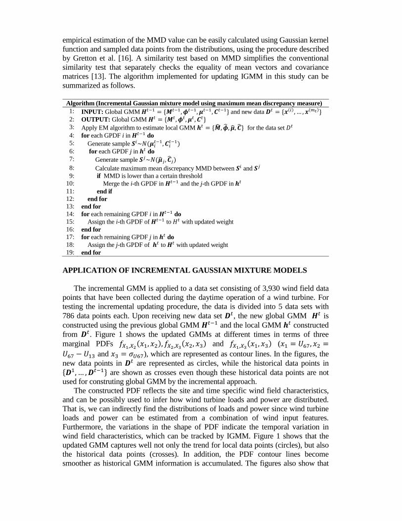
Algorithm (Incremental Gaussian mixture model using maximum mean discrepancy measure)

1: INPUT: Global GMM and new data ( ) ( ) 2: OUTPUT: Global GMM 3: Apply EM algorithm to estimate local GMM for the data set

4: for each GPDF i in do

5: Generate sample (

)

6: for each GPDF j in do

7: Generate sample ( )

8: Calculate maximum mean discrepancy MMD between and

9: if MMD is lower than a certain threshold

10: Merge the i-th GPDF in and the j-th GPDF in

11: end if

12: end for

13: end for

14: for each remaining GPDF i in do

15: Assign the i-th GPDF of to with updated weight

16: end for 17: for each remaining GPDF j in do

18: Assign the j-th GPDF of to with updated weight

19: end for

APPLICATION OF INCREMENTAL GAUSSIAN MIXTURE MODELS

The incremental GMM is applied to a data set consisting of 3,930 wind field data

points that have been collected during the daytime operation of a wind turbine. For

testing the incremental updating procedure, the data is divided into 5 data sets with

786 data points each. Upon receiving new data set , the new global GMM is

constructed using the previous global GMM and the local GMM constructed

from . Figure 1 shows the updated GMMs at different times in terms of three

marginal PDFs ( )

( ) and ( ) (

and ), which are represented as contour lines. In the figures, the

new data points in are represented as circles, while the historical data points in

are shown as crosses even though these historical data points are not

used for construting global GMM by the incremental approach.

The constructed PDF reflects the site and time specific wind field characteristics,

and can be possibly used to infer how wind turbine loads and power are distributed.

That is, we can indirectly find the distributions of loads and power since wind turbine

loads and power can be estimated from a combination of wind input features.

Furthermore, the variations in the shape of PDF indicate the temporal variation in

wind field characteristics, which can be tracked by IGMM. Figure 1 shows that the

updated GMM captures well not only the trend for local data points (circles), but also

the historical data points (crosses). In addition, the PDF contour lines become

smoother as historical GMM information is accumulated. The figures also show that

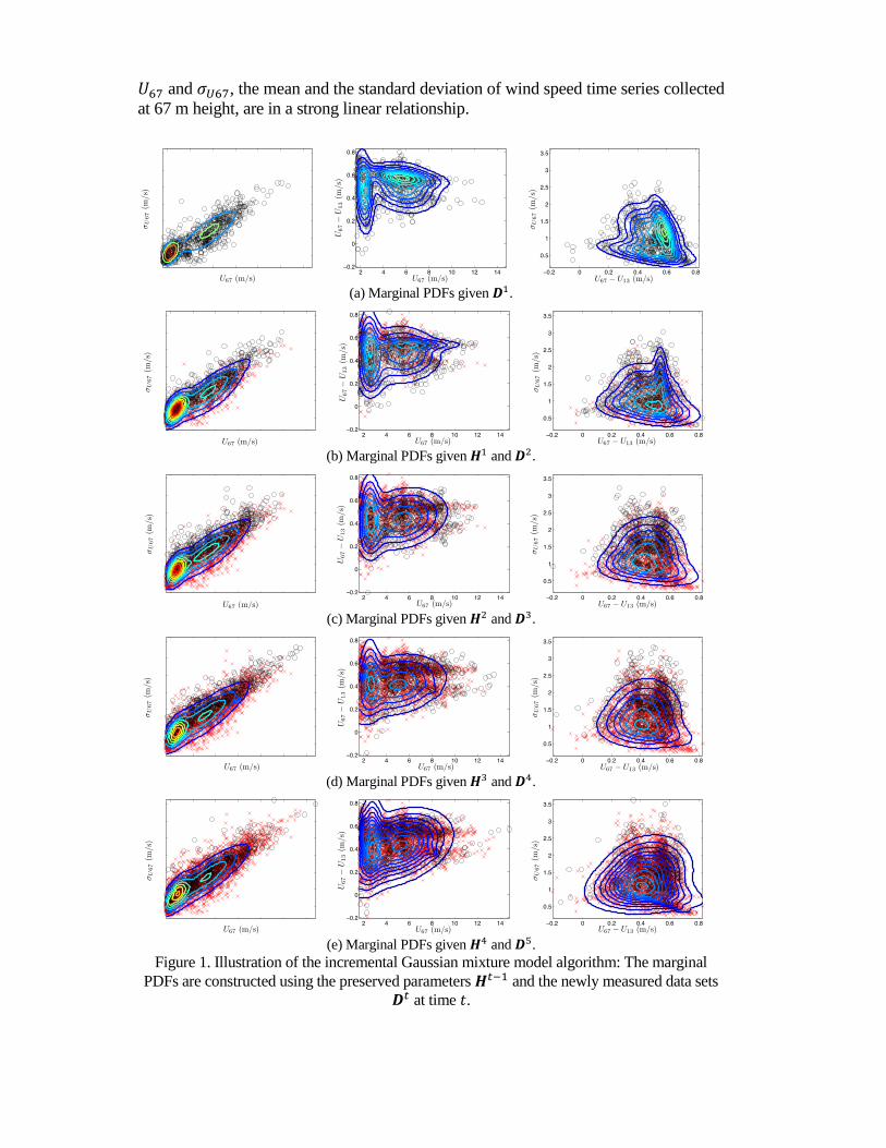
and , the mean and the standard deviation of wind speed time series collected

at 67 m height, are in a strong linear relationship.

(a) Marginal PDFs given .

(b) Marginal PDFs given and .

(c) Marginal PDFs given and .

(d) Marginal PDFs given and .

(e) Marginal PDFs given and .

Figure 1. Illustration of the incremental Gaussian mixture model algorithm: The marginal

PDFs are constructed using the preserved parameters and the newly measured data sets

at time .

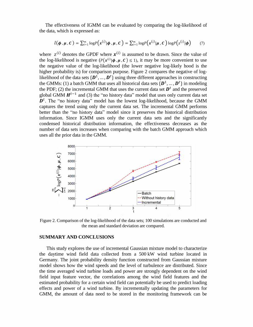
The effectiveness of IGMM can be evaluated by comparing the log-likelihood of

the data, which is expressed as:

( ) ∑ ( ( ) ) ∑ ( ( ) )

( ( ) ) (7)

where ( ) denotes the GPDF where ( ) is assumed to be drawn. Since the value of

the log-likelihood is negative ( ( ( ) ) ), it may be more convenient to use

the negative value of the log-likelihood (the lower negative log-likely hood is the

higher probability is) for comparison purpose. Figure 2 compares the negative of log-

likelihood of the data sets using three different approaches in constructing

the GMMs: (1) a batch GMM that uses all historical data sets in modeling

the PDF; (2) the incremental GMM that uses the current data set and the preserved

global GMM and (3) the “no history data” model that uses only current data set

. The “no history data” model has the lowest log-likelihood, because the GMM

captures the trend using only the current data set. The incremental GMM performs

better than the “no history data” model since it preserves the historical distribution

information. Since IGMM uses only the current data sets and the significantly

condensed historical distribution information, the effectiveness decreases as the

number of data sets increases when comparing with the batch GMM approach which

uses all the prior data in the GMM.

Figure 2. Comparison of the log-likelihood of the data sets; 100 simulations are conducted and

the mean and standard deviation are compared.

SUMMARY AND CONCLUSIONS

This study explores the use of incremental Gaussian mixture model to characterize

the daytime wind field data collected from a 500 kW wind turbine located in

Germany. The joint probability density function constructed from Gaussian mixture

model shows how the wind speeds and the level of turbulence are distributed. Since

the time averaged wind turbine loads and power are strongly dependent on the wind

field input feature vector, the correlations among the wind field features and the

estimated probability for a certain wind field can potentially be used to predict loading

effects and power of a wind turbine. By incrementally updating the parameters for

GMM, the amount of data need to be stored in the monitoring framework can be

significantly reduced. The performance of IGMM is likely dependent on the size of

the data sets, used for updating the GMM. Our future investigation will explore the

tradeoff between the effectiveness of IGMM and the number and size of data sets.

ACKNOWLEDGEMENTS

The wind turbine monitoring activities were partially funded by the German Research

Foundation (DFG) through the grants SM 281/1-1, SM 281/2-1, and HA 1463/20-1.

Any opinions, findings, conclusions, or recommendations are those of the authors and

do not necessarily reflect the views of the DFG.

REFERENCES 1. Park, J, Manuel, L. and Basu, S. 2012. “Toward Understanding Characteristics of the Stable Boundary

Layer that Influence Wind Turbine Loads,” Proc. 50th AIAA Aerospace Sciences Meeting including the

New Horizons Forum and Aerospace Exposition, 01/9/2012.

2. Bao, Y, Beck, J. and Li, H. 2011. “Compressive sampling for accelerometer signals in structural health

monitoring,” Structural Health Monitoring, 10(3): 235-246

3. Huang, Y, Beck, J., Li, H. and Wu, S. 2011. “Robust diagnostics for Bayesian compressive sensing with

applications to structural health monitoring,” Proc. SPIE 7982, Smart Sensor Phenomena, Technology,

Networks, and Systems, 04/15/2011.

4. Smarsly, K., Hartmann, D. and Law, K.H., 2013. “An Integrated Monitoring System for Life-Cycle

Management of Wind Turbines,” International Journal of Smart Structures and Systems (in press).

5. Smarsly, K., Law, K.H. and Hartmann, D., 2011. “Implementation of a multiagent-based paradigm for

decentralized real-time structural health monitoring,” Proceedings of the 2011 ASCE Structures

Congress. Las Vegas, NV, USA, 04/14/2011.

6. Law K.H., Smarsly, K. and Wang, Y., 2013. “Sensor Data Management Technologies,” In: Wang, M. L.,

Lynch, J. P. and Sohn, H. (eds.). Sensor Technologies for Civil Infrastructures: Performance Assessment

and Health Monitoring. Sawston, UK: Woodhead Publishing, Ltd. (in press).

7. Smarsly, K., Law, K.H. and Hartmann, D., 2011. “Implementing a Multiagent-Based Self-Managing

Structural Health Monitoring System on a Wind Turbine,” Proceedings of the 2011 NSF Engineering

Research and Innovation Conference. Atlanta, GA, USA, 01/04/2011.

8. Smarsly, K., Law, K.H. and Hartmann, D., 2013. “A cyberinfrastructure for integrated monitoring and

life-cycle management of wind turbines,” Proceedings of the 20th International Workshop on Intelligent

Computing in Engineering. Vienna, Austria, 06/30/2013.

9. Hartmann, D., Smarsly, K. and Law, K.H., 2011. “Coupling Sensor-Based Structural Health Monitoring

with Finite Element Model Updating for Probabilistic Lifetime Estimation of Wind Energy Converter

Structures, “Proceedings of the 8th International Workshop on Structural Health Monitoring 2011.

Stanford, CA, USA, 09/13/2011.

10. Smarsly, K. and Hartmann, D., 2010. “Agent-Oriented Development of Hybrid Wind Turbine

Monitoring Systems,” Proceedings of ISCCBE International Conference on Computing in Civil and

Building Engineering. Nottingham, UK, 06/30/2010.

11. Lachmann, S., Baitsch, M., Hartmann, D. and Höffer, R. 2009. “Structural lifetime prediction for wind

energy converters based on health monitoring and system identification,” Proceedings of the 5th

European & African Conference on Wind Engineering. Florence, Italy, 07/19/2009.

12. Render, A.R., and Walker, F.H. 1984. “Mixture Densities, Maximum Likelihood and the EM

Algorithm,” SIAM Review, 26(2):195-239.

13. Song, M., and Wang, H. 1996. “Highly efficient incremental estimation of Gaussian mixture models for

online data stream clustering,” Proceedings of the SPIE 5803, Intelligent Computing: Theory and

Applications III, 174, 08/05/2005.

14. Declercq, A. and Piater, H. J. 2008. “Online learning of Gaussian mixture models: a two-level approach,”

Proc. of the Third International Conference on Computer Vision Theory and Applications, 01/22/2008.

15. Stauffer, C. and Grimson, W. 1999. “Adaptive background mixture models for real-time tracking,” In

Computer Vision and Pattern Recognition, 2: 252–258

16. Gretton, A., Borgwardt, K.M., Rasch, M., Scholkopf, B., and Smola, A.J. 2007. “A Kernel Approach to

Comparing Distributions,” Proceedings of the 22nd national conference on Artificial intelligence,

07/22/2007.