APPLICATION OF K-MEANS CLUSTERINGAPPLICATION OF K-MEANS CLUSTERING

• The Matlab function “kmeans()” was used for clustering• The parameters to the function were : 1. The matrix of entire Sea Surface Temperature dataset for a day(v). 2. The number of clusters (n)• The function was tested with the value of n ranging from 3 to 6.• In each case the output was a matrix with unique labels assigned to each cluster. (for ex. For n = 4, the output matrix had clusters identified by labels between 1 and 4).• The matrix was mapped onto the original SST data and visualized.• Statistical data extracted from the clusters included

1. Mean value of each cluster.2. Standard deviation.3. The size of each cluster.

• Analysis of the statistical data was done over data for the entire month of August 2003.• The analysis involved a difference in clustering approach where pixels that migrated between clusters were identified , between n and n+1.• The pattern of migration was analyzed. Interesting features were visible between n = 3 and n = 4.

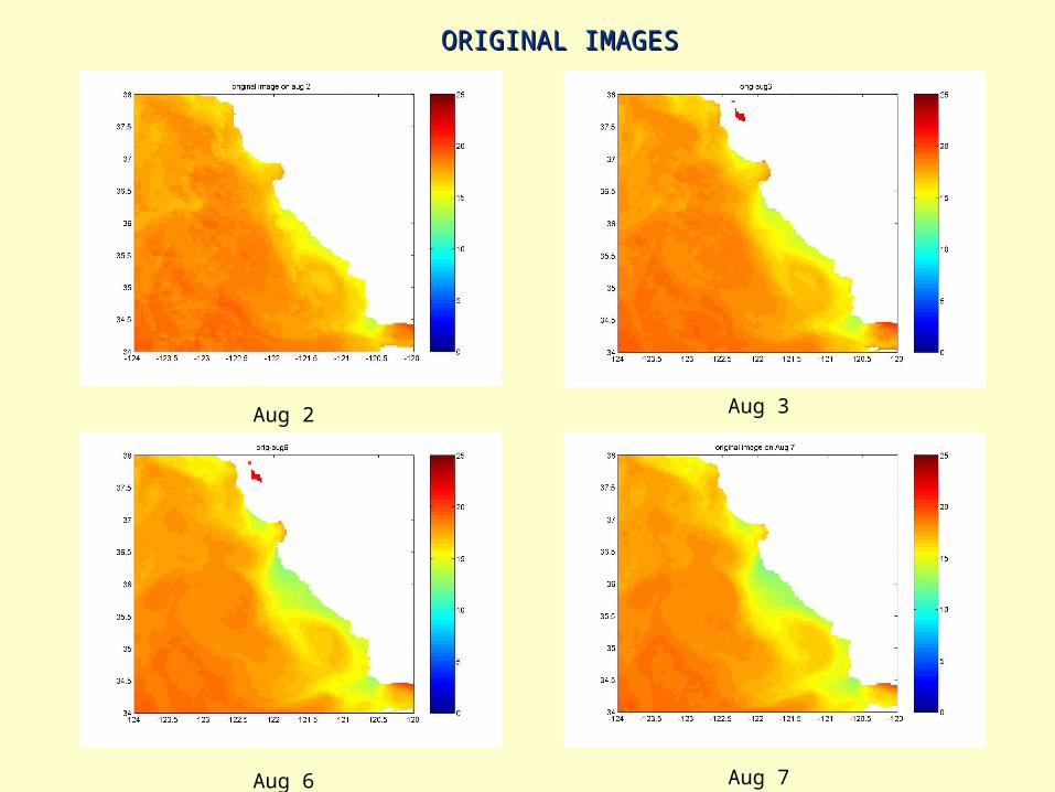
ORIGINAL IMAGESORIGINAL IMAGES

Aug 2 Aug 3

Aug 6 Aug 7

ORIGINAL IMAGESORIGINAL IMAGES

Aug 8 Aug 9

Aug 10 Aug 11

Aug 12 Aug 14

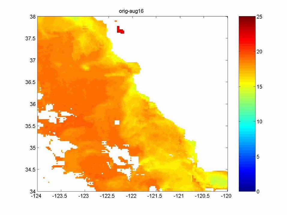
Aug 16

ORIGINAL IMAGESORIGINAL IMAGES

Aug 2 – 4 clusters Aug 2 – 5 clusters

Original – Aug 2

A B

C

D

A’B’

C’

D’

E

OBSERVATION:OBSERVATION: * There is no upwelling region on this day

CLUSTERINGCLUSTERING

Aug 7 – 4 clusters Aug 7 – 5 clusters

Original – Aug 7 Upwelling overlaid

A B

C

D

A’B’

E

C’

D’

CLUSTERINGCLUSTERING

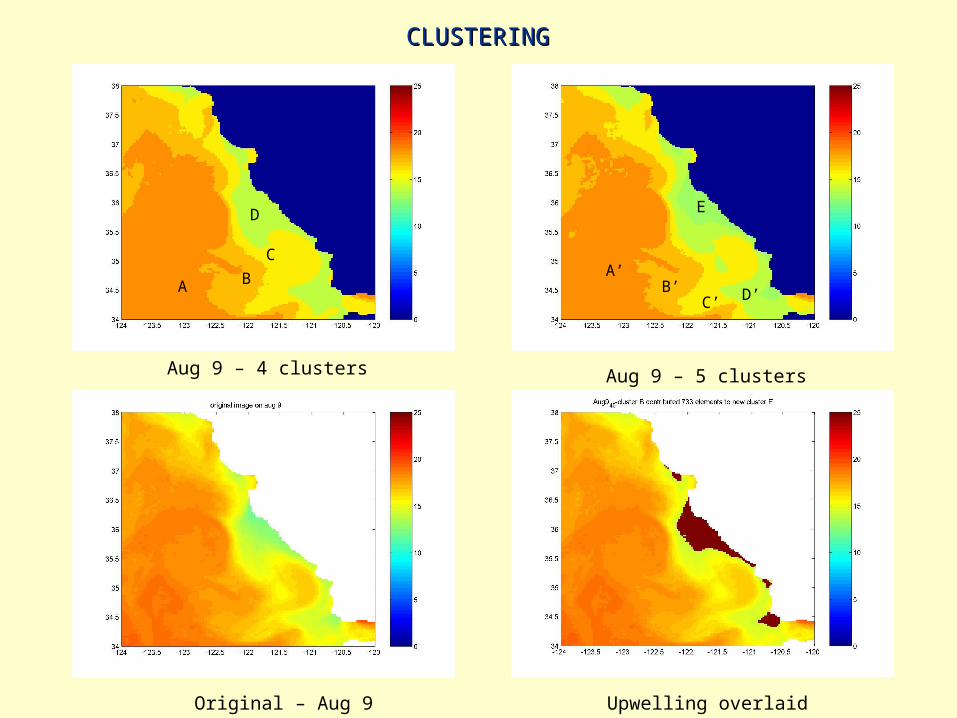
Aug 9 – 4 clusters Aug 9 – 5 clusters

Original – Aug 9 Upwelling overlaid

A B

C

D

A’B’

C’ D’

E

CLUSTERINGCLUSTERING

Aug 9 – 4 clusters Aug 9 – 5 clusters

Original – Aug 9 Upwelling overlaid

A’B’

C’ D’

E

A B

C

D

CLUSTERINGCLUSTERING

•Detection•Feature Segmentation•Boundary identification ( For detection of fronts and eddies)

Original – Aug 11 Overlay on original

DIFFERENCE IN CLUSTERINGDIFFERENCE IN CLUSTERING

0

0.2

0.4

0.6

0.8

1

1.2

1 3 5 7 9 11 13 15 17 19 21

Series1Y

XX – axis : Number of observationsY – axis : Difference in mean values between cluster number ‘4’ for n =4 and cluster number ‘5’ for n = 5.

• The difference in mean values between the clusters with the minimum mean temperature for 4 clusters and 5 clusters respectively, were plotted for the month of August 2003.• The upwelling region being a relatively colder region would fall in the cluster with the minimum temperature.• The plot showed a steady increase and then decrease during the upwelling period.

Analysis of Data