53

Corresponding Author. Email: umutokkan@balikesir.edu.tr

Application of Levenberg-Marquardt Optimization Algorithm Based

Multilayer Neural Networks for Hydrological Time Series Modeling

Umut Okkan a

aDepartment of Civil Engineering, Balikesir University-Turkey

Email: umutokkan@balikesir.edu.tr

(Received March 03, 2011; in final form June 24, 2011)

Abstract. Recently, Artificial Neural Networks (ANN), which is mathematical modeling

tools inspired by the properties of the biological neural system, has been typically used in

the studies of hydrological time series modeling. These modeling studies generally include

the standart feed forward backpropagation (FFBP) algorithms such as gradient-descent,

gradient-descent with momentum rate and, conjugate gradient etc. As the standart FFBP

algorithms have some disadvantages relating to the time requirement and slow

convergency in training, Newton and Levenberg-Marquardt algorithms, which are

alternative approaches to standart FFBP algorithms, were improved and also used in the

applications. In this study, an application of Levenberg-Marquardt algorithm based ANN

(LM-ANN) for the modeling of monthly inflows of Demirkopru Dam, which is located in

the Gediz basin, was presented. The LM-ANN results were also compared with gradient-

descent with momentum rate algorithm based FFBP model (GDM-ANN). When the

statistics of the long-term and also seasonal-term outputs are compared, it can be seen that

the LM-ANN model that has been developed, is more sensitive for prediction of the

inflows. In addition, LM-ANN approach can be used for modeling of other hydrological

components in terms of a rapid assessment and its robustness.

Keywords: Levenberg-Marquardt optimization algorithm, Artificial neural networks,

Hydrological time series modeling

AMS subject classifications: 92B20, 62M10

1. Introduction

The application of water resource engineering

methods to evaluate the potential of water

resource and the decision making strategies of

water resource management, such as

droughtflood analysis, irrigation, reservoir

performances based on probability of failure and,

the development of integrated river basin models

under the certain climate scenarios, needs the

forecasting of streamflow data and modeling of

rainfall-runoff relations. In this context, the

examination of hydrological processes and

causalities of these processes deepens our

understanding of modeling. Especially, the recent

and apparent impacts of climate change have also

popularized these models.

A basin can be considered as a system that

transforms the rainfall to runoff. The modeling of

this system can be set up to obtain the relation of

the transformation by making simplifying

assumptions because a basin has very

complicated and uncertain components. There are

different classifications presented in the literature

to qualify basin models which include system

definitions, area-time scales and solution

techniques. But in general, there are three main

approaches in representing the basin systems:

white-box models (physical based distributed

models), the gray-box models (conceptual

models) and the blackbox models [1]. The white

and gray-box models aim to simulate physical

creation mechanism in the ways of each of theirs

components, such as surface, subsurface and

groundwater flow, infiltration, percolation, and

An International Journal of Optimization

and Control: Theories & Applications

Vol.1, No.1, pp.53-63 (2011) © IJOCTA

ISSN 2146-0957 http://www.ijocta.com

54 Vol.1, No.1, (2011) © IJOCTA

evapotranspiration. The relevant parameters of

these components for a certain basin are

determined by different optimization techniques.

However, in terms of uncertainties, data

requirements and complexities of model

parameters, they can not use in some

applications. Because of uncertainties and

complexities in these modeling studies, the basin

may be also considered as the black-box models

which are applied to associate basin inputs and

desired outputs without detailed consideration

about the physical processes of the phenomena.

In this context, conventional statistical models

are commonly used in applications which contain

regression analyses, curve fitting approaches and

stochastic autoregressive models [2-9]. In

addition to these, artificial neural networks

(ANNs) are also employed to streamflow

modeling [10-15]. The ANNs can be considered

as complex and nonlinear regression models

structured between basin inputs (precipitation,

temperature, evaporation etc.) and basin output

“streamflow” data. Although there are several

ANN techniques, feed forward backpropagation

(FFBP) algorithm based models used in

applications typically. A number of ANN studies

have been reported in literature. Some of them

are given. Minns and Hall (1996) prepared a

FFBBP algorithm based ANN model by using

synthetic data set to forecast streamflows.

Campalo et al.(1999) developed an ANN model

to analyze and forecast the behavior of the river

Tagliamento, in Italy [16]. Mendez et al. (2004),

Kisi (2005) and Okkan and Mollamahmutoglu

(2010a) investigated the performance of ANN

and autoregressive models in prediction of

streamflow [15, 17, 18]. They were shown that

ANN methods yielded better results than

autoregressive models. Cigizoglu (2003) also

used an autoregressive model which was

employed to generate synthetic monthly flows

[14]. These generated values were used as the

training sets of ANNs to forecast the observed

Goksu River monthly mean flows in the East

Mediterranean part of Turkey. According to this,

the forecasting results were compared with the

ANN performance when only a limited number

of observed flows were employed in the training

data sets. Increasing the data sets in the training

stage improved the forecasting performance

significantly. In addition to FFBP algorithms,

Generalized Regression Neural Networks [19,

20] and Radial Basis Neural Networks [21-23]

studies were also used in streamflow predictions.

Briefly, all of these studies shown that the ANN

is probably the most successful black box tool

which is capable of modeling complex and

uncertain relationships between input and output

variables without the detailing of the physical

process.

In the study presented, an application of

Levenberg-Marquardt algorithm based ANN

(LM-ANN) for the modeling of monthly inflows

of Demirkopru Dam, which is located in the

Gediz Basin, was presented. The LM-ANN

results were also compared with gradient-descent

with momentum rate algorithm based FFBP

model (GDM-ANN).

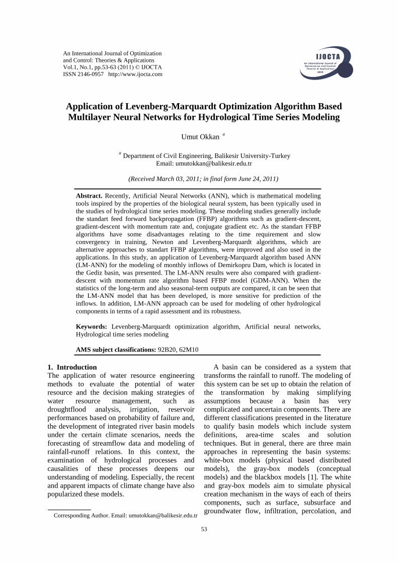
2.The Multilayer Neural Networks

The basic concept of the multilayer neural

networks is that they are typically made up of

single neurons. And in the multilayer neural

networks, the neurons are organized in the form

of layers (Figure 1).

The first and last layer of multilayer neural

networks is called the input and the output layers

respectively.The input layer does not perform any

computations, but only serves to feed the input

data to the hidden layer which is between the

input and output layers.

Figure 1. A multilayer neural network structure

[18]

In general, there can be any number of hidden

layers in the multilayer neural networks

structures. However, from practical applications,

only one or two hidden layers are used. In

addition to this, the number of hidden layers and

also the number of neurons of hidden layers can

be determined by trial and error [24-26]. There are also three important components of

a multilayer neural network structure: weights,

summing function and activation function. The

importance and functionality of the inputs on

Application of Levenberg-Marquardt Optimization Algorithm Based Multilayer Neural Networks… 55

neural network models are obtained with weights

(W).

So the success of the model depends on the

precise and correct determination of weight

values. The summing function (net) acts to add

all outputs; that is, each neuron input is

multiplied by the weights and then summed.

After computing the sum of weighted inputs for

all neurons, the activation function f (.) serves to

limit the amplitude of these values. The

activation functions are usually continuous, non-

decreasing and bounded functions.

Various types of the activation function are

possible but generally sigmoid function is

preferred in applications [26]. This activation

function generates outputs between 0 and 1 as the

input signal goes from negative to positive

infinity.

(.)

1(.)

1f

e

(1)

In addition to the structure and its components

of multilayer neural networks, the running

procedure is also important which involves

typically two phases; forward computing and

backward computing.

In forward computing, each layer uses a

weight matrix (W (v)

, for v =1, 2) associated with

all the connections made from the previous layer

to the next layer (Figure 1). The hidden layer has

the weight matrix (1) hxnW R , the output layer’s

weight matrix is (2) mxhW R . Given the network

input vector 1nxx R , the output of the hidden

layer 1

,1

hx

outx R can be written as

(1) (1) (1) (1)

,1 [ ] [ ]outx f net f W x (2)

which is the input to the output layer. The output

of the output layer, which is the response (output)

of the network 1

,2

mx

outy x R , can be written

as

(2) (2) (2) (2)

,2 ,1[ ] [ ]out outy x f net f W x (3)

Substituting (Eq.2) into (Eq.3) for xout,1 gives the

final output y = xout,2 of the network as

(2) (2) (1) (1)[ [ ]]y f W f W x (4)

After the phase of forward computing,

backward computing which depending on the

algorithms to adjust weights is used in the

multilayer neural networks. The process of

adjusting these weights to minimize the

differences between the actual and the desired

output values is called training or learning the

network. If these differences (error) are higher

than the desired values, the errors are passed

backwards through the weights of the network. In

ANN terminology, this phase is also called the

backpropagation algorithm. Once the comparison

error is reduced to an acceptable level for the

whole training set, the training period ends, and

the network is also tested for another known

input and output data set in order to evaluate the

generalization capability of the ANN [24, 26].

Depending on the techniques to train ANN

models, different back propagation algorithms

have been developed. In this study, the

Levenberg-Marquardt algorithm (LM-ANN) was

used for training of the network. The Levenberg-

Marquardt algorithm is a second order nonlinear

optimization technique that is usually faster and

more reliable than any other standart back

propagation techniques [27-29] and it is similar

to Newton’s method [30, 31].

3. The Levenberg-Marquardt Algorithm

The Levenberg-Marquardt optimization

algorithm represents a simplified version of

Newton’s method [31] applied to the training

multilayer neural networks [30, 32]. Consider the

multilayer neural network shown in Figure 1, the

running of the network training can be viewed as

finding a set of weights that minimized the error

(ep) for all samples in the training set (Q). If the

performances function is a sum of squares of the

errors as

2 2

1 1

1 1( ) ( ) ( ) ,

2 2

P P

p p p

p p

E W d y e P mQ

(5)

where Q is the total number of training samples,

m is the number of output layer neurons, W

represents the vector containing all the weights in

the network, yp is the network output, and dp is

the desired output.

When training with the Levenberg-Marquardt

optimization algorithm, the changing of weights

ΔW can be computed as follows

1 [ ]T T

k k k k kW J J I J e (6)

where J is the Jacobian. matrix, I is the identify

matrix, µ is the Marquardt parameter which is to

be updated using the decay rate β depending on

the outcome. In particular, µ is multiplied by the

decay rate β (0<β<1) whenever E(W) decreases,

while µ is divided by β whenever E(W) increases

in a new step (k).

The LM-ANN training process can be

illustrated in the following pseudo-codes,

56 Vol.1, No.1, (2011) © IJOCTA

1. Initialize the weights and µ (µ = 0.001 is

appropriate).

2. Compute the sum of squared errors over all

inputs, E(W).

3. Compute the Jacobian matrix J.

4. Solve Eq.6 to obtain the changing of

weights ΔW.

5. Recompute the sum of squared errors E(W)

using 1

( 1) [ ]T T

k k k k k k kW W J J I J e

as the

trial W, and judge

IF trial E(W) < E(W) in Step 2, THEN 1

( 1)

( 1)

[ ]

( 0.1)

T T

k k k k k k k

k k

W W J J I J e

go back to Step 2.

ELSE

( 1) /k k

go back to Step 4.

END IF

4. Application

The application area covers the Demirkopru

Dam’s basin which is located in the Aegean

region of Turkey. The study region has typical

Mediterranean climate characteristics.

Demirkopru Dam’s basin is also called the

Upper Gediz which has four rivers (Demirci,

Deliinis, Selendi and Murat) located upstream of

the dam with a total drainage area of 6590 km2

(Figure 2).

Figure 2 The streamflow and the meteorological

stations in the study area

LM-ANN modeling was applied on the

observed data of selected 5 meteorological

stations and 4 streamflow gauging stations

(Table 1).

Table 1 Selected meteorological and streamflow

gauging stations in the study area

For the study region, the monthly data set of

streamflows (106 m

3) at each station was obtained

from EIE (the General Directorate of Electrical

Power Resources Survey and Development

Administration of Turkey) and then summed.

Thus, monthly inflows of Demirkopru dam was

determined for the period from 1977 to 2006. The

monthly data sets of precipitation at Demirci,

Icikler, Kiransih, Fakili and Gediz meteorological

stations were obtained from DMI (the State

Meteorological Organization of Turkey) and DSI

(the General Directorate of State Hydraulic

Works of Turkey) and the monthly mean areal

precipitation values determined from these

meteorological stations by using Thiessen

polygons. The monthly data sets of temperature

at Demirci and Gediz meteorological stations

were also obtained from DMI (the State

Meteorological Organization of Turkey) and the

monthly mean areal temperature values computed

by using arithmetical mean values from these

meteorological stations for the period from

January 1977 to December 2006.

In the modeling application, 30 years (January

1977-December 2006) input-output data were

used and divided into training and testing periods

by proportions of 2/3 (January 1977- December

1996) and 1/3 (January 1997-December 2006),

respectively. Before presenting the input-output

data to ANN, the all data set were scaled to the

range 0-1 so that the different input signal had the

same numerical range. The training and the

testing subsets were scaled to the range of 0-1

using the equation zt = (xt-xmin)/(xmax-xmin), where

xt is the unscaled data, zt is scaled data, and xmax

and xmin are the maximum and minimum values

Type of Stations Station Names Station Numbers

Meteorological

Demirci DMI 17746

İcikler DSI 05-018

Kiransih DSI 05-016

Fakili DSI 05-012

Gediz DMI 17750

Streamflow

Demirci EIE 522

Deliinis EIE 515

Selendi EIE 514

Gediz EIE 523

Application of Levenberg-Marquardt Optimization Algorithm Based Multilayer Neural Networks… 57

of the unscaled data, respectively. Then, the

output values of the networks, which were in the

range of 0-1, were converted to real-scaled values

using the equation xt = zt (xmax - xmin) + xmin.

Because of the scaling range, the sigmoid

function was selected as the activation function

which generates outputs between 0 and 1.

In training, the number of hidden layers, the

number of the neurons in the hidden layers and

Marquardt parameters were determined after

trying various network structures. The network

structure providing the best result, i.e., the

minimum root mean square errors, RMSE (Eq. 7),

and the maximum determination coefficients, R2

(Eq. 8) was also employed for the testing period.

2

1

1( )

T

t t

t

RMSE d yT

(7)

2 2

2 1 1

2

1

( ) ( )

( )

T T

t mean t t

t t

T

t mean

t

d d d y

R

d d

(8)

where T is the number of training or testing

samples, yt is the network output, dt is the

observed (desired) data in the tth time period, and

dmean is the mean over the observed periods.

The modeling study started with the network-

input data consisting of the concurrent monthly

rainfall and temperature and the corresponding

inflows at Demirkopru Dam as an output from

the network. The maximum possible model

determinations (R2) and the minimum root mean

square errors (RMSE) obtained with two inputs

and one output, network was 70.94 % and 37.74

(106 m

3) and 61.17 % and 46.09 (10

6 m

3) for the

training and testing periods respectively. The

number of neurons in the hidden layer was tried

between 2 and 20 and the one with 12 neurons

gave the best performance on the testing data. To

develop the performance of the LM-ANN model,

antecedent rainfalls were included in the input.

The best performance for the model

determinations was obtained with 9 neurons in

the hidden layer with a concurrent monthly

rainfall, temperature and three antecedent

rainfalls used as input. With these inputs,

determinations of 93.31 % and 82.19 % were

obtained for the training and testing periods

respectively. When two and three antecedent

rainfalls were added to the model, the

performance of training period improved, but in

terms of root mean square errors, the

performance for the testing period was found to

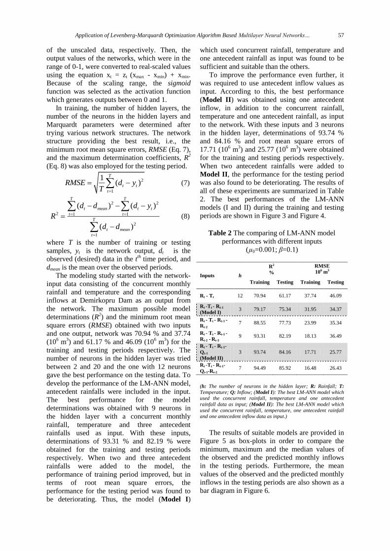
be deteriorating. Thus, the model (Model I)

which used concurrent rainfall, temperature and

one antecedent rainfall as input was found to be

sufficient and suitable than the others.

To improve the performance even further, it

was required to use antecedent inflow values as

input. According to this, the best performance

(Model II) was obtained using one antecedent

inflow, in addition to the concurrent rainfall,

temperature and one antecedent rainfall, as input

to the network. With these inputs and 3 neurons

in the hidden layer, determinations of 93.74 %

and 84.16 % and root mean square errors of

17.71 (106 m

3) and 25.77 (10

6 m

3) were obtained

for the training and testing periods respectively.

When two antecedent rainfalls were added to

Model II, the performance for the testing period

was also found to be deteriorating. The results of

all of these experiments are summarized in Table

2. The best performances of the LM-ANN

models (I and II) during the training and testing

periods are shown in Figure 3 and Figure 4.

Table 2 The comparing of LM-ANN model

performances with different inputs

(µ0=0.001; β=0.1)

Inputs h

R2

%

RMSE

106 m3

Training Testing Training Testing

Rt - Tt 12 70.94 61.17 37.74 46.09

Rt -Tt - Rt-1

(Model I) 3 79.17 75.34 31.95 34.37

Rt - Tt - Rt-1 -

Rt-2 7 88.55 77.73 23.99 35.34

Rt - Tt - Rt-1 -

Rt-2 - Rt-3 9 93.31 82.19 18.13 36.49

Rt - Tt - Rt-1- Qt-1

(Model II)

3 93.74 84.16 17.71 25.77

Rt -Tt - Rt-1-

Qt-1-Rt-2 7 94.49 85.92 16.48 26.43

(h: The number of neurons in the hidden layer; R: Rainfall; T:

Temperature; Q: Inflow; (Model I): The best LM-ANN model which used the concurrent rainfall, temperature and one antecedent

rainfall data as input; (Model II): The best LM-ANN model which

used the concurrent rainfall, temperature, one antecedent rainfall and one antecedent inflow data as input.)

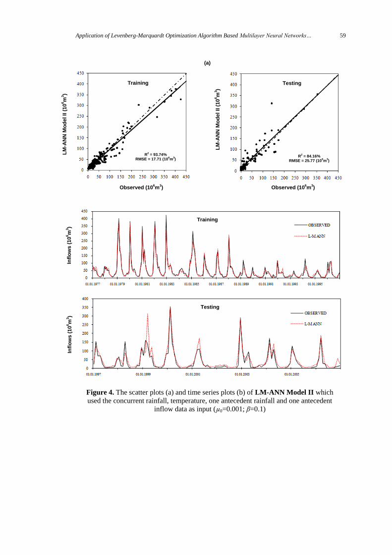
The results of suitable models are provided in

Figure 5 as box-plots in order to compare the

minimum, maximum and the median values of

the observed and the predicted monthly inflows

in the testing periods. Furthermore, the mean

values of the observed and the predicted monthly

inflows in the testing periods are also shown as a

bar diagram in Figure 6.

58 Vol.1, No.1, (2011) © IJOCTA

Training Testing

R2 = 79.17%

RMSE = 31.95 (106m

3)

R2 = 75.34%

RMSE = 34.37 (106m

3)

LM

-AN

N M

od

el I

(10

6m

3)

LM

-AN

N M

od

el I

(10

6m

3)

Observed (106m

3)

Observed (106m

3)

(a)

(b)

Infl

ow

s (

10

6m

3)

Infl

ow

s (

10

6m

3)

Training

Testing

Figure 3 The scatter plots (a) and time series plots (b) of LM-ANN Model I which used

the concurrent rainfall, temperature and one antecedent rainfall data as input

(µ0=0.001; β=0.1)

Observed (106m

3)

Application of Levenberg-Marquardt Optimization Algorithm Based Multilayer Neural Networks… 59

(a)

Training Testing

LM

-AN

N M

od

el II (

10

6m

3)

R2 = 93.74%

RMSE = 17.71 (106m

3)

R2 = 84.16%

RMSE = 25.77 (106m

3)

LM

-AN

N M

od

el II (

10

6m

3)

Observed (106m

3) Observed (10

6m

3)

Infl

ow

s (

10

6m

3)

Infl

ow

s (

10

6m

3)

Training

Testing

Figure 4. The scatter plots (a) and time series plots (b) of LM-ANN Model II which

used the concurrent rainfall, temperature, one antecedent rainfall and one antecedent

inflow data as input (µ0=0.001; β=0.1)

60 Vol.1, No.1, (2011) © IJOCTA

When the box-plots were examined, in terms

of the median values of the observed and the

predicted monthly inflows, the all models were

fitted well. But the results of some months

(especially November and December) in Model

II which used the one antecedent inflow data as

input was much better than the Model I.

When the box-plots were also compared, in

terms of the extreme (maximum and minimum)

values of the observed and the predicted monthly

inflows, it was noticed that there were different

results.

For example the extreme values of March

were fitted by Model I. However, the results of

November and December in Model II were much

better than the Model I as well as in terms of

monthly means (See Figure 6).

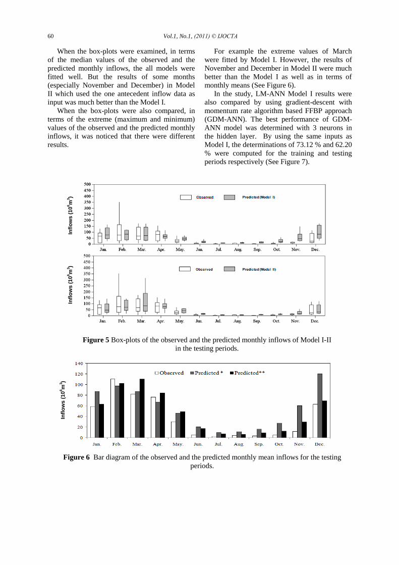
In the study, LM-ANN Model I results were

also compared by using gradient-descent with

momentum rate algorithm based FFBP approach

(GDM-ANN). The best performance of GDM-

ANN model was determined with 3 neurons in

the hidden layer. By using the same inputs as

Model I, the determinations of 73.12 % and 62.20

% were computed for the training and testing

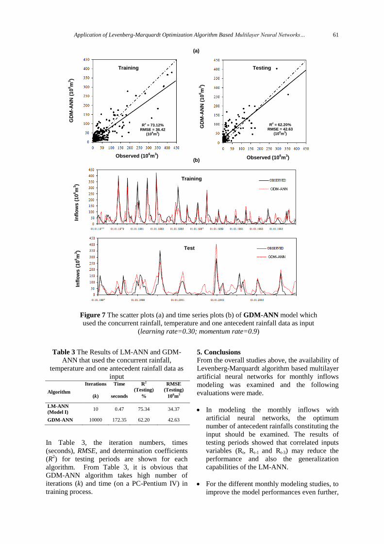
periods respectively (See Figure 7).

Figure 5 Box-plots of the observed and the predicted monthly inflows of Model I-II

in the testing periods.

Figure 6 Bar diagram of the observed and the predicted monthly mean inflows for the testing

periods.

Infl

ow

s (

10

6m

3)

Infl

ow

s (

10

6m

3)

Infl

ow

s (

10

6m

3)

Application of Levenberg-Marquardt Optimization Algorithm Based Multilayer Neural Networks… 61

Table 3 The Results of LM-ANN and GDM-

ANN that used the concurrent rainfall,

temperature and one antecedent rainfall data as

input

Algorithm

Iterations Time R2

(Testing)

RMSE

(Testing)

(k) seconds % 106m3

LM-ANN

(Model I) 10 0.47 75.34 34.37

GDM-ANN 10000 172.35 62.20 42.63

In Table 3, the iteration numbers, times

(seconds), RMSE, and determination coefficients

(R2) for testing periods are shown for each

algorithm. From Table 3, it is obvious that

GDM-ANN algorithm takes high number of

iterations (k) and time (on a PC-Pentium IV) in

training process.

5. Conclusions

From the overall studies above, the availability of

Levenberg-Marquardt algorithm based multilayer

artificial neural networks for monthly inflows

modeling was examined and the following

evaluations were made.

In modeling the monthly inflows with

artificial neural networks, the optimum

number of antecedent rainfalls constituting the

input should be examined. The results of

testing periods showed that correlated inputs

variables (Rt, Rt-1 and Rt-3) may reduce the

performance and also the generalization

capabilities of the LM-ANN.

For the different monthly modeling studies, to

improve the model performances even further,

(b)

Infl

ow

s (

10

6m

3)

Infl

ow

s (

10

6m

3)

Training

Test

Figure 7 The scatter plots (a) and time series plots (b) of GDM-ANN model which

used the concurrent rainfall, temperature and one antecedent rainfall data as input

(learning rate=0.30; momentum rate=0.9)

GD

M-A

NN

(10

6m

3)

Observed (106m

3)

Training

R2 = 73.12%

RMSE = 36.42 (10

6m

3)

Testing

(a)

GD

M-A

NN

(10

6m

3)

Observed (106m

3)

R2 = 62.20%

RMSE = 42.63 (10

6m

3)

62 Vol.1, No.1, (2011) © IJOCTA

it may be required to use antecedent inflow

values as input.

Further, the time required for training by the

LM-ANN is not only the lowest but also only

a fraction of the time taken by GDM-ANN

algorithms.

This was also proved with this study, that

LM-ANN is the one of the most successful

black box techniques which is capable of

rainfall-runoff modeling without the detailing

of the physical process and can be also used

for modeling of other hydrological

components in terms of a rapid assessment

and its robustness.

6. References

[1] Abbott, M.B. and Refsgaard, J.C. Distributed

Hydrological Modeling. Kluver Academic

Publishers, Dordrecht. 17-39 (1996).

[2] Spolia, S.K., and Chander, S. Modeling of

surface runoff systems by an ARMA model.

Journal of Hydrology, 22, 317-332 (1974).

[3] Sim C. H. A Mixed Gamma ARMA(1,1) Model

for River Flow Time Series. Water Resources

Research, 23(1), 32-36 (1987).

[4] Fernandez B., and Salas J.D. Gamma

Autoregressive Models for Stream- Flow

Simulation. Journal of Hydrologic Engineering,

116 (11), 1403-1414 (1990).

[5] Cigizoglu, K., and Bayazit, M. Application of

Gamma Autoregressive Model to Analysis of

Dry Periods. Journal of Hydrologic Engineering,

3(3), 218-221 (1998).

[6] Yurekli, K., and Ozturk, F. Stochastic Modeling

of Annual Maximum and Minimum Streamflow

of Kelkit Stream, Water International, 28, 433-

441 (2003).

[7] Yurekli, K., Kurunc, A., and Ozturk, F.

Application of Linear Stochastic Models to

Monthly Flow Data of Kelkit Stream, Ecological

Modeling, 183, 67-75 (2005a).

[8] Yurekli, K., Kurunc, A., and Ozturk, F. Testing

The Residuals of an ARIMA Model on The

Cekerek Stream Watershed in Turkey, Turkish

Journal of Engineering and Environmental

Sciences, 29, 61-74 (2005b).

[9] Kurunc, A., Yurekli, K., and Cevik, O.

Performance of Two Stochastic Approaches for

Forecasting Water Quality and Streamflow Data

from Yeşilιrmak River, Turkey, Environmental

Modeling & Software, 20, 1195-1200 (2005).

[10] Raman, H. and Sunilkumar, N., Multivariate

modeling of water resources time series using

artificial neural networks, Hydrological Sciences

Journal, 40, 2, 145-163 (1995).

[11] Hsu, K., Gupta, H.V. and Sorooshian, S.,

Artificial neural network modelling of the

rainfall runoff process, Water Res. Research, 31,

2517-2530 (1995).

[12] Minns, A.W. and Hall, M.J., Artificial neural

networks as rainfall runoff models Hydrological

Sciences Journal, 41, 3, 399-417 (1996).

[13] Tokar, A.S. and Johnson, P.A., Rainfall runoff

modeling using artificial neural networks,

Journal of Hydrologic Engineering, 4, 3, 232-239

(1999).

[14] Cigizoglu, H.K., Incorporation of ARMA models

into flow forecasting by artificial neural

networks, Environmetrics, 14, 4, 417-427 (2003).

[15] Kisi, O., Daily river flow forecasting using

artificial neural networks and auto-regressive

models. Turkish Journal of Engineering and

Environmental Sciences, 29, 9–20 (2005).

[16] Campolo, M., Andreussi, P. ve Soldati, A., River

flood forecasting with a neural network model,

Water Resources Research, 35, 1191-1197

(1999).

[17] Méndez, M. C., Manteiga, W.G., Bande, M.F.

Sánchez J.M.P. and Calderón

R.L., Modeling of

the monthly and daily behavior of the runoff of

the Xallas river using Box–Jenkins and neural

networks methods. Journal of Hydrology, 296,

38-58 (2004).

[18] Okkan, U., Mollamahmutoğlu, A. Çoruh Nehri

günlük akımlarının yapay sinir ağları ile tahmin

edilmesi, Süleyman Demirel Üniversitesi Fen

Bilimleri Enstitüsü Dergisi, 14, 3, 251-261

(2010a).

[19] Cigizoglu H.K., Application of the Generalized

Regression Neural Networks to Intermittent

Flow Forecasting and Estimation. Journal of

Hydrologic Engineering, 10(4), 336-341 (2005a).

[20] Cigizoglu H.K., Generalized regression neural

networks in monthly flow forecasting. Civil

Engineering and Environmental Systems. 22 (2),

71-84 (2005b).

[21] Fernando, D.A.K., and Jayawardena, A.W.,

Runoff forecasting using RBF networks with

OLS algorithm, Journal of Hydrologic

Engineering 3, 3, 203-209 (1998).

Application of Levenberg-Marquardt Optimization Algorithm Based Multilayer Neural Networks… 63

[22] Lin, G., and Chen, L., A non-linear rainfall-

runoff model using radial basis function network,

Journal of Hydrology, 289, 1-8 (2004).

[23] Okkan, U., Serbeş Z.A., Radyal tabanlı yapay

sinir ağları yaklaşımı ile günlük akımların

modellenmesi, İnşaat Mühendisleri Odası İzmir

Şube Bülteni, 155, 26-29 (2010).

[24] Haykin, S. Neural Networks: A Comprehensive

Foundation. MacMillan. New York (1994).

[25] Skapura, D. M. Building Neural Networks,

Addison-Wesley, New York (1996)

[26] Ham, F., and Kostanic, I., Principles of

Neurocomputing for Science and Engineering.

Macgraw-Hill. USA (2001).

[27] Kisi, O., Multi-layer perceptrons with

Levenberg–Marquardt training algorithm for

suspended sediment concentration prediction and

estimation. Hydrological Sciences Journal 49 (6),

1025–1040 (2004).

[28] Cigizoglu, H.K., and Kisi, O., Flow prediction by

three back propagation techniques using k-fold

partitioning of neural network training data.

Nordic Hydrology 36 (1), 49–64 (2005).

[29] Okkan, U., Mollamahmutoğlu, A. Yiğitler Çayı

günlük akımlarının yapay sinir ağları ve

regresyon analizi ile modellenmesi, Dumlupınar

Üniversitesi Fen Bilimleri Enstitüsü Dergisi, 23,

33-48 (2010b).

[30] Hagan, M.T., and Menhaj, M.B., Training feed

forward techniques with the Marquardt

algorithm. IEEE Transactions on Neural

Networks 5 (6), 989–993 (1994).

[31] Marquardt, D., An algorithm for least squares

estimation of non-linear parameters. Journal of

the Society for Industrial and Applied

Mathematics 11 (2), 431–441 (1963).

[32] Hagan, M.T., Demuth, H.P., and Beale, M.,

Neural Network Design. PWS Publishing,

Boston (1996).

Umut OKKAN (M.Sc.) is a Research

Assistant at Balikesir University - Engineering

and Architecture Faculty - Department of Civil

Engineering. His research interests are

hydrology, water resources, climate models,

statistics, stochastic modeling, artificial

intelligence techniques, and designing of water

distribution systems.

64 Vol.1, No.1, (2011) © IJOCTA