Int J Theor PhysDOI 10.1007/s10773-014-2035-7

Application of Lie Algebroid Structures to Unificationof Einstein and Yang-Mills Field Equations

N. Elyasi ·N. Boroojerdian

Received: 16 September 2013 / Accepted: 28 January 2014© Springer Science+Business Media New York 2014

Abstract Yang-Mills field equations describe new forces in the context of Lie groups andprinciple bundles. It is of interest to know if the new forces and gravitation can be describedin the context of algebroids. This work was intended as an attempt to answer last question.The basic idea is to construct Einstein field equation in an algebroid bundle associated tospace-time manifold. This equation contains Einstein and Yang-Mills field equations simul-taneously. Also this equation yields a new equation that can have interesting experimentalresults.

Keywords Lie algebra · Lie algebroid · Connection · Metric · Curvature · Gravitation ·Field equation · Unification

Mathematical Subject Classifications (2010) 81V22 · 83E15

1 Introduction

Einstein field equation describes gravitational forces, and Yang-Mills field equationsdescribe other forces. Principle bundles on a space-time and principle connections are mainapparatus for introducing and compromising Yang-Mills theory and GR [1]. This methodas in Kaluza-KLien theory [4, 6] make us to assume some extra dimension in space-time.Here we propose some other method that is capable of describing gravitation and new forcessimultaneously .In addition this method needs no extra dimension in space-time. The mainidea of this method is enriching tangent bundle of the space-time by a Lie algebra and makean algebroid structure. In our method, we need no extra dimension in space-time manifold,but we add some extra dimension to tangent bundle of space-time. Our approach is differentfrom Kaluza-KLien theory, since first we have no extra dimension in space-time, second

N. Elyasi (�)Department of Mathematics and Computer Sciences, Kharazmi University, Karaj, Irane-mail: elyasi82@aut.ac.ir

N. BoroojerdianDepartment of Mathematics & Computer Science, Amirkabir University of Technology, Tehran, Irane-mail: broojerd@aut.ac.ir

Int J Theor Phys

we use different mathematical structures, third our method is more general and containsresults of Yang-Mills theory. Of course, our results is very near to that of Kaluza-KLien andYang-Mills theory, but our method is different.

In [3] we have introduced a Lie algebroid bundle that is an extension of tangent bundleof some space-time. This extension can be expressed by

TM =⋃

p

TpM ⊕ IR = TM ⊕ IR

In that structure we could unify Einstein and Maxwell equations. In that method IR playsthe role of a trivial Lie algebra. In this paper we replace IR with an arbitrary Lie algebrað. One of the physical interpretations of this work, is replacing the unified Maxwell andEinstein field equations in [3] with the unified Yang-Mills and Einstein field equations.

2 Connection Form and its Curvature Form

In this section M is a smooth manifold and U ∈ XM and ð is a Lie algebra and ω ∈A1(M,ð). ω has some relations to connection forms on principle bundles and may be usedto define a connection on some trivial vector bundles, so we call it a ð-valued connectionform on M(note this is just a name and it doesn’t mean that ω satisfies the connection formconditions). Let W be vector space and ρ : ð×W −→ W , ρ(h, v) = h.v be a Lie algebrarepresentation of ð on W .

We can use ω to define a connection on the trivial vector bundle M×W by the followingequation.

X ∈ C∞(M,W), ∇ωUX = U(X)+ ω(U).X (1)

By U(X) we mean Lie derivation of X with respect to U . As an important example consideradjoint representation of ð on itself. If ξ ∈ C∞(M,ð), then from (1) the next equationholds.

∇ωU ξ = U(ξ)+ [ω(U), ξ ]

Proposition 2.1 If ξ ∈ C∞(M,ð) and X ∈ C∞(M,W) , then we have

∇ωU (ξ.X) = (∇ω

U ξ)

.X + ξ.∇ωUX (2)

Proof Since the action of ð on W is bilinear, then

U(ξ.X) = U(ξ).X+ ξ.U(X)

Now the following computations show the result.

∇ωU (ξ.X) = U(ξ.X)+ ω(U).(ξ.X)

= U(ξ).X+ ξ.U(X)+ ω(U).(ξ.X)− ξ.(ω(U).X)+ ξ.(ω(U).X)

= U(ξ).X+ ξ.(U(X)+ ω(U).X)+ [ω(U), ξ ].X= (∇ω

U ξ)

.X + ξ.∇ωUX

In the case of M × ð, if ξ, η ∈ C∞(M,ð) , then

∇ωU [ξ, η] =

[∇ωU ξ, η

] + [

ξ,∇ωUη

]

Int J Theor Phys

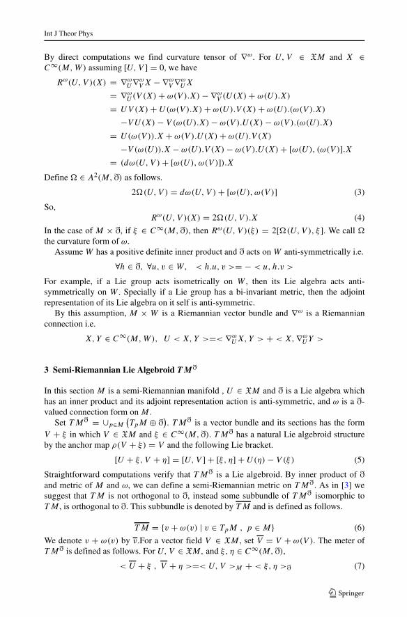
By direct computations we find curvature tensor of ∇ω. For U, V ∈ XM and X ∈C∞(M,W) assuming [U, V ] = 0, we have

Rω(U, V )(X) = ∇ωU∇ω

V X −∇ωV∇ω

UX

= ∇ωU(V (X)+ ω(V ).X)−∇ω

V (U(X)+ ω(U).X)

= UV (X)+ U(ω(V ).X)+ ω(U).V (X)+ ω(U).(ω(V ).X)

−VU(X)− V (ω(U).X)− ω(V ).U(X)− ω(V ).(ω(U).X)

= U(ω(V )).X + ω(V ).U(X)+ ω(U).V (X)

−V (ω(U)).X− ω(U).V (X)− ω(V ).U(X)+ [ω(U), (ω(V )].X= (dω(U,V )+ [ω(U), ω(V )]).X

Define � ∈ A2(M,ð) as follows.

2�(U,V ) = dω(U, V )+ [ω(U), ω(V )] (3)

So,Rω(U, V )(X) = 2�(U,V ).X (4)

In the case of M × ð, if ξ ∈ C∞(M,ð), then Rω(U, V )(ξ) = 2[�(U,V ), ξ ]. We call �the curvature form of ω.

Assume W has a positive definite inner product and ð acts on W anti-symmetrically i.e.

∀h ∈ ð, ∀u, v ∈ W, < h.u, v >= − < u, h.v >

For example, if a Lie group acts isometrically on W , then its Lie algebra acts anti-symmetrically on W . Specially if a Lie group has a bi-invariant metric, then the adjointrepresentation of its Lie algebra on it self is anti-symmetric.

By this assumption, M × W is a Riemannian vector bundle and ∇ω is a Riemannianconnection i.e.

X,Y ∈ C∞(M,W), U < X,Y >=< ∇ωUX, Y > + < X,∇ω

UY >

3 Semi-Riemannian Lie Algebroid TMð

In this section M is a semi-Riemannian manifold , U ∈ XM and ð is a Lie algebra whichhas an inner product and its adjoint representation action is anti-symmetric, and ω is a ð-valued connection form on M .

Set TMð = ∪p∈M(

TpM ⊕ ð)

. TMð is a vector bundle and its sections has the formV + ξ in which V ∈ XM and ξ ∈ C∞(M,ð). TMð has a natural Lie algebroid structureby the anchor map ρ(V + ξ) = V and the following Lie bracket.

[U + ξ, V + η] = [U, V ] + [ξ, η] + U(η)− V (ξ) (5)

Straightforward computations verify that TMð is a Lie algebroid. By inner product of ðand metric of M and ω, we can define a semi-Riemannian metric on TMð. As in [3] wesuggest that TM is not orthogonal to ð, instead some subbundle of TMð isomorphic toTM , is orthogonal to ð. This subbundle is denoted by TM and is defined as follows.

TM = {v + ω(v) | v ∈ TpM , p ∈ M} (6)

We denote v + ω(v) by v.For a vector field V ∈ XM , set V = V + ω(V ). The meter ofTMð is defined as follows. For U, V ∈ XM, and ξ, η ∈ C∞(M,ð),

< U + ξ , V + η >=< U, V >M + < ξ, η >ð (7)

Int J Theor Phys

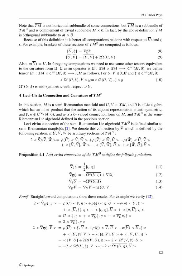
Note that TM is not horizontal subbundle of some connections, but TM is a subbundle ofTMð and is complement of trivial subbundle M × ð. In fact, by the above definition TM

is orthogonal subbundle to M × ð.Because of this definition it is better all computations be done with respect to Us and ξ

s. For example, brackets of these sections of TMð are computed as follows.

[U, ξ ] = ∇ωU ξ (8)

[U,V ] = [U, V ] + 2�(U,V ) (9)

Also, ρ(U) = U . In foregoing computations we need to use some other tensors equivalentto the curvature form �. � as an operator is � : XM × XM −→ C∞(M,ð). we definetensor �a : XM × C∞(M,ð) −→ XM as follows. For U, V ∈ XM and ξ ∈ C∞(M,ð),

< �a(U, ξ), V >M=< �(U,V ), ξ >ð (10)

�a(U, ξ) is anti-symmetric with respect to U .

4 Levi-Civita Connection and Curvature of TMð

In this section, M is a semi-Riemannian manifold and U, V ∈ XM , and ð is a Lie algebrawhich has an inner product that the action of its adjoint representation is anti-symmetric,and ξ, η ∈ C∞(M,ð), and ω is a ð- valued connection form on M , and TMð is the semi-Riemannian Lie algebroid defined in the previous section.

Levi-civita connection of the semi-Riemannian Lie algebroid TMð is defined similar tosemi-Riemannian manifolds [2]. We denote this connection by ∇ which is defined by thefollowing relation, if U, V , W be arbitrary sections of TMð :

2 < ∇U

V , W >= ρ(U) < V , W > +ρ(V ) < W, U > −ρ(W) < U, V >

+ < [U, V ], W > − < [V , W ], U > + < [W, U ], V >

Proposition 4.1 Levi-civita connection of the TMð satisfies the following relations.

∇ξ η = 1

2[ξ, η] (11)

∇Uξ = −�a(U, ξ)+∇ωU ξ (12)

∇ξU = −�a(U, ξ) (13)∇UV = ∇UV +�(U,V ) (14)

Proof Straightforward computations show these results. For example we verify (12).

2 < ∇Uξ, η > = ρ(U) < ξ, η > +ρ(ξ) < η,U > −ρ(η) < U, ξ >

+ < [U, ξ ], η > − < [ξ, η], U > + < [η,U ], ξ >

= U < ξ, η > + < ∇ωU ξ, η > − < ∇ω

Uη, ξ >

= 2 < ∇ωU ξ, η >

2 < ∇Uξ,V > = ρ(U) < ξ, V > +ρ(ξ) < V ,U > −ρ(V ) < U, ξ >

+ < [U, ξ ], V > − < [ξ, V ], U > + < [V ,U ], ξ >

= < [V,U ] + 2�(V,U), ξ >= 2 < �a(V, ξ),U >

= −2 < �a(U, ξ), V >= −2 < �a(U, ξ), V >

Int J Theor Phys

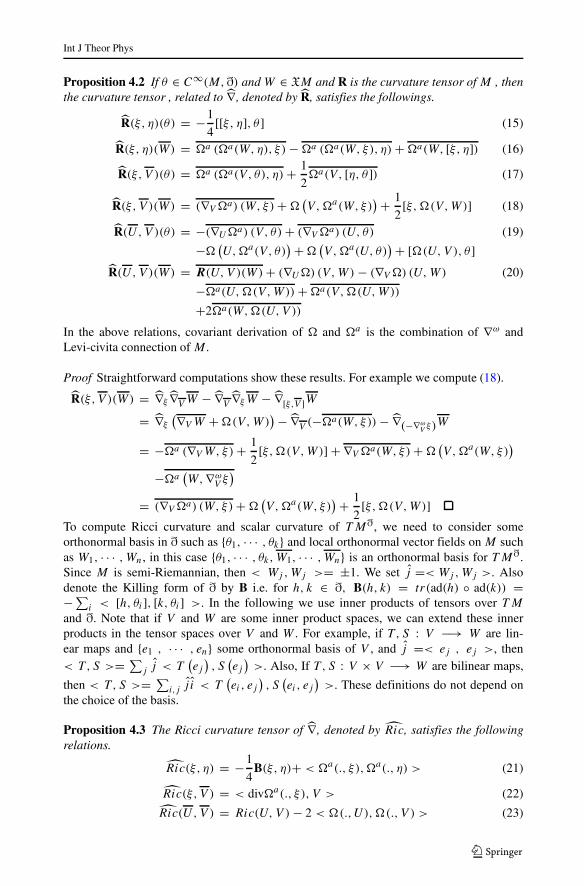
Proposition 4.2 If θ ∈ C∞(M,ð) and W ∈ XM and R is the curvature tensor of M , thenthe curvature tensor , related to ∇, denoted by R, satisfies the followings.

R(ξ, η)(θ) = −1

4[[ξ, η], θ ] (15)

R(ξ, η)(W) = �a (�a(W, η), ξ )−�a (�a(W, ξ), η)+�a(W, [ξ, η]) (16)

R(ξ, V )(θ) = �a (�a(V, θ), η)+ 1

2�a(V, [η, θ ]) (17)

R(ξ, V )(W) = (∇V �a) (W, ξ)+�(

V,�a(W, ξ)) + 1

2[ξ, �(V,W)] (18)

R(U, V )(θ) = −(∇U�a) (V, θ)+ (∇V �a) (U, θ) (19)

−�(

U,�a(V, θ)) +�

(

V,�a(U, θ))+ [�(U,V ), θ ]

R(U, V )(W) = R(U, V )(W)+ (∇U�) (V,W)− (∇V �) (U,W) (20)

−�a(U,�(V,W))+�a(V,�(U,W))

+2�a(W,�(U,V ))

In the above relations, covariant derivation of � and �a is the combination of ∇ω andLevi-civita connection of M .

Proof Straightforward computations show these results. For example we compute (18).

R(ξ, V )(W) = ∇ξ∇VW − ∇V

∇ξW − ∇[ξ,V ]W

= ∇ξ

(∇VW +�(V,W)) − ∇V (−�a(W, ξ))− ∇(−∇ω

V ξ)W

= −�a (∇VW, ξ)+ 1

2[ξ,�(V,W)] + ∇V �a(W, ξ)+�

(

V,�a(W, ξ))

−�a(

W,∇ωV ξ

)

= (∇V �a) (W, ξ)+�(

V,�a(W, ξ)) + 1

2[ξ,�(V,W)]

To compute Ricci curvature and scalar curvature of TMð, we need to consider someorthonormal basis in ð such as {θ1, · · · , θk} and local orthonormal vector fields on M suchas W1, · · · ,Wn, in this case {θ1, · · · , θk,W1, · · · ,Wn} is an orthonormal basis for TMð.Since M is semi-Riemannian, then < Wj ,Wj >= ±1. We set j =< Wj ,Wj >. Alsodenote the Killing form of ð by B i.e. for h, k ∈ ð, B(h, k) = tr(ad(h) ◦ ad(k)) =−∑

i < [h, θi], [k, θi] >. In the following we use inner products of tensors over TM

and ð. Note that if V and W are some inner product spaces, we can extend these innerproducts in the tensor spaces over V and W . For example, if T , S : V −→ W are lin-ear maps and {e1 , · · · , en} some orthonormal basis of V , and j =< ej , ej >, then< T,S >= ∑

j j < T(

ej)

, S(

ej)

>. Also, If T , S : V × V −→ W are bilinear maps,

then < T, S >= ∑

i,j j i < T(

ei , ej)

, S(

ei, ej)

>. These definitions do not depend onthe choice of the basis.

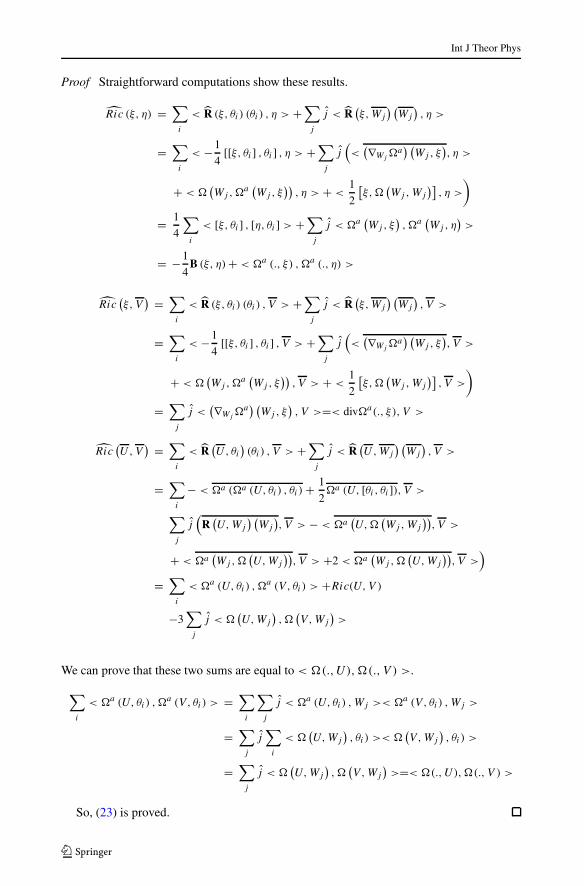
Proposition 4.3 The Ricci curvature tensor of ∇, denoted by Ric, satisfies the followingrelations.

Ric(ξ, η) = −1

4B(ξ, η)+ < �a(., ξ ),�a(., η) > (21)

Ric(ξ, V ) = < div�a(., ξ ), V > (22)Ric(U, V ) = Ric(U, V )− 2 < �(.,U),�(., V ) > (23)

Int J Theor Phys

Proof Straightforward computations show these results.

Ric (ξ, η) =∑

i

< R (ξ, θi ) (θi ) , η > +∑

j

j < R(

ξ,Wj

) (

Wj

)

, η >

=∑

i

< −1

4[[ξ, θi ] , θi ] , η > +

∑

j

j(

<(∇Wj

�a) (

Wj, ξ)

, η >

+ < �(

Wj,�a(

Wj, ξ))

, η > + <1

2

[

ξ,�(

Wj,Wj

)]

, η >

)

= 1

4

∑

i

< [ξ, θi ] , [η, θi ] > +∑

j

j < �a(

Wj, ξ)

,�a(

Wj, η)

>

= −1

4B (ξ, η)+ < �a (., ξ) ,�a (., η) >

Ric(

ξ, V) =

∑

i

< R (ξ, θi ) (θi ) , V > +∑

j

j < R(

ξ,Wj

) (

Wj

)

, V >

=∑

i

< −1

4[[ξ, θi ] , θi ] , V > +

∑

j

j(

<(∇Wj

�a) (

Wj, ξ)

, V >

+ < �(

Wj,�a(

Wj, ξ))

, V > + <1

2

[

ξ,�(

Wj,Wj

)]

, V >

)

=∑

j

j <(∇Wj

�a) (

Wj, ξ)

, V >=< div�a(., ξ), V >

Ric(

U,V) =

∑

i

< R(

U, θi)

(θi ) , V > +∑

j

j < R(

U,Wj

) (

Wj

)

, V >

=∑

i

− < �a (�a (U, θi ) , θi )+ 1

2�a (U, [θi , θi ]), V >

∑

j

j(

R(

U,Wj

) (

Wj

)

, V > − < �a(

U,�(

Wj,Wj

))

, V >

+ < �a(

Wj,�(

U,Wj

))

, V > +2 < �a(

Wj,�(

U,Wj

))

, V >)

=∑

i

< �a (U, θi ) ,�a (V , θi ) > +Ric(U, V )

−3∑

j

j < �(

U,Wj

)

,�(

V,Wj

)

>

We can prove that these two sums are equal to < �(.,U),�(., V ) >.

∑

i

< �a (U, θi ) ,�a (V , θi ) > =

∑

i

∑

j

j < �a (U, θi ) ,Wj >< �a (V, θi ) ,Wj >

=∑

j

j∑

i

< �(

U,Wj

)

, θi ) >< �(

V,Wj

)

, θi ) >

=∑

j

j < �(

U,Wj

)

,�(

V,Wj

)

>=< �(.,U),�(., V ) >

So, (23) is proved.

Int J Theor Phys

Proposition 4.4 If R be the scalar curvature of M then the scalar curvature related to ∇,denoted by R, satisfies the following relation.

R = R− < �,� > −1

4tr(B) (24)

Proof

R =∑

i

Ric (θi, θi )+∑

j

Ric(

Wj ,Wj

)

=∑

i

(

−1

4B (θi, θi )+ < �a (., θi) ,�

a (., θi) >

)

+∑

j

(

Ric(

Wj ,Wj

) − 2 < �(

.,Wj

)

, �(

.,Wj

)

>)

= −1

4tr(B)+ R+ < �a,�a > −2 < �,� >

Since < �a,�a >=< �,� >, the proposition is proved.

5 Application to General Relativity and Yang-Mills Theory

In this section M is a space-time, and g and ω are the same as in the previous section. We caninterpret ω as potential for new relativistic forces in a similar way that Yang-Mills theorydescribes. In this interpretation, geodesics of TMð must show the path of point particlesinfluenced by gravitation and new forces.

Definition 5.1 A smooth curve α : I −→ TMð is called a velocity-curve whenever thereexist a curve α : I −→ M such that ρ(α) = α′.

In this case, there exists a curve ξ : I −→ ð such that α(t) = α′(t) + ξ(t). A smoothmap β : I −→ TMð is called along the velocity-curve α, whenever ρ(β(t)) ∈ Tα(t)M i.e.π ◦ ρ ◦ α = π ◦ ρ ◦ β. The covariant derivation of a map along a velocity-curve α(t)) isdefinable. A velocity-curve α is called geodesic whenever ∇α α = 0.

Proposition 5.2 A velocity-curve α(t) = α′(t) + ξ(t) is geodesic iff∇α′(t)α′(t) = 2�a(α′(t), ξ(t)) and ξ(t) is parallel along α(t) with respect to ∇ω.

Proof

∇α α = ∇α′(t)+ξ(t)

α′(t)+ ξ(t)

= ∇α′(t)α

′(t)+ ∇α′(t)ξ(t)+ ∇ξ(t)α′(t)+ ∇ξ(t)ξ(t)

= ∇α′(t)α′(t)−�a(α′(t), ξ(t))+∇ωα′(t)ξ(t)−�a(α′(t), ξ(t))

Therefore, ∇α α = 0 iff ∇α′(t)α′(t) = 2�a(α′(t), ξ(t)) and ∇ωα′(t)ξ(t) = 0.

In the case ð = IR, ξ represents ratio of charge to mass and 2�a(α′(t), ξ(t)) representselectromagnetic force exerted to the particle [3]. So we can consider elements of ð as vectorcharges (divided by mass) and 2�a(α′(t), ξ(t)) can be considered as the force produced bythese vector charges.

Int J Theor Phys

To find more detailed and explicit information of new forces and their analogy to elec-tromagnetism, it is better to write connection form ω and its curvature � with respect to thebase {θ1, · · · , θk}.

ω = ωiθi ωi ∈ A1(M) i = 1, · · · , k� = �iθi �i ∈ A2(M) i = 1, · · · , k

Suppose [θi, θj ] = Clijθl , since 2�(U,V ) = dω(U, V ) + [ω(U), ω(V )], by computation

we find:2�l = dωl + Cl

ijωi ∧ ωj (25)

Set �ai (U) = �a(U, θi). �a

i is the 1-1-form equivalent to 2-form �i .

Corollary 5.3 Let α(t) = α′(t)+ ξ(t) be a geodesic and ξ(t) = ξ i(t)θi , then

∇α′(t)α′(t) = 2ξ l(t)�a

l (α′(t)) (26)

ξ l′(t) = Cl

ij ξi(t)ωj (α′(t)) (27)

We can interpret ξ l as l−th charge and �al as l−th electromagnetism field and

2ξ l(t)�al (α

′(t)) as sum of the the forces exerted by these fields. Of course these forces arenot independent and (25) shows these forces are dependent to each other and are componentsof a more general force.

Set Bij = B(

θi, θj)

. Ric and R with respect to the base {θ1, · · · , θk}, can be written asfollows:

Ric(

θi, θj) = −1

4Bij+ < �a

i ,�aj > (28)

Ric(

θi, V) = < div�a

i , V > (29)

Ric(

U,V) = Ric(U, V )− 2

∑

i

< �ai (U),�a

i (V ) > (30)

R = R −∑

i

< �ai ,�

ai > −1

4

∑

i

Bii (31)

In the case of ð = IR, energy-momentum tensor of electromagnetism forces in a suitable

system of measurement,(

c = 1 , G = 1 , ε0 = 116π

)

[3], is defined as follows.

Telec = 1

4π

(

< �a(.),�a(.) > −1

4< �a,�a > g

)

(32)

g is the tensor metric of M . We can extend this definition and define i−th energy-momentum tensor of ω by

Tωi = 1

4π

(

< �ai (.),�

ai (.) > −1

4< �a

i , �ai > g

)

(33)

Define the whole energy-momentum tensor of ω by T ω = ∑

i Tωi . This definition dose not

depend on the choice of θi , in fact:

Tω(U, V ) = 1

4π

(

< �a(U, .),�a(V, .) > −1

4< �a,�a >< U, V >

)

(34)

Denote the meter of TMð by g. To construct a suitable field equation that produces Einsteinfield equation, we should imitate Einstein field equation in the context of this algebroid

Int J Theor Phys

bundle. So by analogy, we can consider G = Ric − 12Rg as the extended Einstein tensor.

This tensor in block form looks like the following matrix.(

Ric − 12Rg + 1

8 tr(B)g − 8πT ω div�a

tdiv�a λij

)

λij = −1

4Bij+ < �a

i ,�aj > −1

2Rδij

Note that R = R− < �,� > − 14 tr(B). Now, we can construct vacuum field equation as

follows.

Ric − 1

2Rg = 0 (35)

This equation yields R = 0 and is equivalent to Ric = 0 and has the followingconsequences.

Ric − 1

2Rg + 1

8tr(B)g = 8πT ω (36)

div�ai = 0 (37)

< �ai ,�

aj > = 1

4Bij (38)

Note that in λij , we have R = 0, so λij = 0 yields (38). Two of these equations are Einsteinand Yang-Mills field equations in vacuum and we find a third new (38), that may havenew results. Moreover, Einstein field equation naturally yields a cosmological constant thatdepends on inner product of ð and by re-scaling can be adapted its value to experimentaldata.

Particles are modeled by representations of the Lie algebra ð. Suppose a representationof ð on some inner product vector spaces W that ð acts on W anti-symmetrically. AnyX ∈ C∞(M,W) is called a particle field. We can consider ρ =< X,X > as density ofthis particle field. Charge density of a particle field can be considered as a smooth functionη : M −→ ð.

In order to construct the field equation including matter, we should extend the conceptof energy-momentum tensor of matter, and we do this the same as [3]. Let T mass be theordinary energy-momentum tensor of the particle field. For every observer Z, T mass(Z,Z)

is the energy of the particle measured by Z [5]. We can define current of this particle fieldto be J ∈ A1(M,ð) such that for every observer Z, J (Z) is the vector charge of the particlefield measured by Z.

T mass and J are parts of the extended energy-momentum tensor which is denoted by T .In fact for U, V ∈ XM and ξ ∈ C∞(M,ð), we define:

T (U, V ) = T mass(U, V ) , T (U, ξ ) =< J(U), ξ >

To complete the construction of T , similar to [3], we need a symmetric 2-tensor on ð. Itseems we should consider 1

ρη⊗η for this tensor. Because, in the case ð = IR in [3] we have

good reason for it and it is very natural. Of course, only results of this choice and experiencecan show that this choice is true or not. So we propose, T (ξ1, ξ2) = 1

ρ< ξ1, η >< ξ2, η >,

and T be defined as follows:

T =(

T mass tJ

J 1ρη⊗ η

)

(39)

Int J Theor Phys

Now, we can write the Einstein field equation in this structure as following.

Ric − 1

2Rg = 8πT (40)

This equation contains three following equations.

Ric − 1

2Rg + 1

8tr(B)g = 8π

(

T ω + T mass) (41)

tdiv� = 8πJ (42)

λij = 8πηiηj

ρ(43)

The first two equations are Einstein and Yang-Mills field equations and third equation isnew and may have new results. Equation (40) makes Einstein and Yang-Mills theory into aunified theory in the context of Lie algebroid structures.

6 Conclusion

These constructions retrieve Yang-Mills theory in the context of Lie algebroid structuresand they need no principle bundle and principle connection. This theory is more simple anddoes not make any extra dimension in space-time, instead it enriches tangent bundle by aLie algebra and makes a Lie algebroid and replaces tangent bundle by this Lie algebroid.

Of course, this theory does not contain quantum effects and internal structures of par-ticles. This theory must be improved such that internal structures of particles determinedensity and vector charge density naturally.

References

1. Bleeker, D.: Gauge Theory and Variational Principles. Addison-Wesley (1981)2. Boucetta, M.: Riemannian Geometry of Lie Algebroids. (2008). arXiv:0806.3522v23. Elyasi, N., Boroojerdian, N.: Affine metrics and algebroid structures: application to general relativity

and unification. Int. J. Theor. Phys. (2012). doi:10.1007/s10773-012-1197-44. Overdain, J.M.: Kaluza-KLien Gravity. (1998). arXiv:gr-qc/9805018v15. Sachs, R.K., Wu, H.: General Relativity for Mathematicians. Springer-Verlag, New York (1977)6. Wesson, P.S.: Space Time Matter: Modern Kaluza-KLien Theory: Word Scientific