APPLICATION OF LINEAR ALGEBRA IN

COMBINATORICS

Xilogiannis EvangelosAdvisor : Mihalis Kolountzakis

University of CreteDepartment of mathematics

May 2010

2

Acknowledgements

I would like to thank my adviser professor Prof. Mihalis Kolountzakis forthe assistance he has provided me and also thank the other two members of mycommittee Profs Theodoulos Garefalakis and Eleni Tzanaki.

Contents

1 Introduction 5

2 Useful Lemmas 7

3 The Kakeya Problem 11

4 The Joints Problem 17

5 Discrete geometry problems 21

6 Extremal set theory 27

7 Hilbert’s Third problem 33

8 References 37

3

4 CONTENTS

Chapter 1

Introduction

In the following pages we will examine the use of linear algebra in combinatorics.More precisely we will look at some theorems from the area of discrete geom-etry,extremal combinatorics and finite fields constructions. The dates of theresults span from the beginning of the 20th century (the Dehn theorem) to re-cent years (the Dvir theorem) . The tools used although may appear elementarythey give powerful and interesting results .

5

6 CHAPTER 1. INTRODUCTION

Chapter 2

Useful Lemmas

First we will prove some theorems that we will make frequent use of.

Note In the following pages F will denote a finite field.

Definition Let U be a m×m matrix over R. If for all nonzero vectors x itis true that xUxT > 0 we say that the matrix is positive definite. If it is truethat xUxT ≥ 0 we say that the matrix is positive semidefinite.

Definition Let V be a linear space over Q. A linear function is a map

f : V → Q

with the property that for all a, b ∈ V we have

f(a+ b) = f(a) + f(b)

We also know that if two elements a, b ∈ V are linearly independent there is alinear function that f(a) = 0 and f(b) = 1.

Definition A symmetricm×mmatrix B with real entries is positive semidef-inite if for any x ∈ Rm the quadratic form xBTx is nonnegative. If in additionthe only case the quadratic form xBTx vanishes is only when x is itself zerothen B is positive definite.

Theorem 1. (Schwartz 1980) Let f ∈ F [x1, .., xn] be a non zero polynomialwith degree d and Ω ⊆ F be a set with |Ω| = N . Let Z(f,Ω) denote the set ofroots from Ωn. Then

|Z(f,Ω)| ≤ dNn−1

Proof. By induction on n, the number of variables.For n = 1 the number of roots cannot exceed the degree thus |Z(f,Ω)| ≤ d.For n ≥ 2 we write f in terms of the powers of xn

7

8 CHAPTER 2. USEFUL LEMMAS

f(x1, ..., xn) = g0 + g1xn + g2x2n + ...+ gkx

kn (2.1)

where gi ∈ F [x1, ..xn−1] , deg gi ≤ d − i and gk is not the zero polynomial.We choose an element (a1, ..., an) of Z(f,Ω) at random. There are two possiblecases :

1) gk(a1, ..an−1) = 0As deg(gk) ≤ d − k by the inductive hypothesis the number of roots of gk inthe subset Ωn−1 is at most (d− k)Nn−2. Thus the possible maximal number ofthose tuples is ≤ (d− k)Nn−1 .

2) gk(a1, ..an−1) 6= 0In this case we bound the number of tuples simply by Nn−1. Since an mustnow be a root of the non zero polynomial f of degree k, the number of possiblechoices for an is at most k. Hence this case results in at most kNn−1 roots of f.

The two upper bounds add to total of dNn−1 completing the proof.

The following lemma is an immediate consequence of the above.

Lemma 1. Small degree lemma A polynomial in F d of degree less thanq = |F | cannot vanish everywhere unless it is the zero polynomial

Proof. Let P be a non zero polynomial. Since deg(P ) ≤ |F |−1 by the Schwartztheorem the number of its roots cannot exceed the number (|F | − 1)|F |n−1. Byassumption this is a contradiction thus P must be identically zero.

We will now establish some criteria regarding the linear independence ofpolynomials.

Lemma 2. (Diagonal Criterion) For i = 1, ..,m let fi : Ω −→ F be afunction and ai ∈ Ω elements such

fi(aj)6= 0 if i = j;= 0 if i 6= j.

then f1, ...fm are linearly independent members of the space FΩ

Proof. Letm∑i=1

λifi(x) = 0

be a linear relation between the fi. We substitute aj for the variable x andwhat remains is λjfj(aj) = 0 which implies that λj = 0 for every j.

9

Thus the linear relation under consideration is the trivial one.

Lemma 3. (Triangular Criterion ) For i = 1, ...m let fi : Ω −→ F be afunction and ai ∈ Ω elements such

fi(aj)6= 0 if i = j;= 0 if i < j.

then f1, ...fm are linearly independent members of the space FΩ.

Proof. For a contradiction we assume there exists a nontrivial linear relation∑mi=1 λifi = 0 between the fi. Let i0 be the greater i such that λi 6= 0. We

substitute ai0 for the variable on each side. By the above condition for thefi(aj) all but one terms vanish and what remains is

λi0fi0(ai0) = 0

. Which implies that λi0 = 0. Which is a contradiction.

We will now present some classic and useful results in enumerate combina-torics.

Lemma 4. The number of integer solutions to the equation

x1 + ...+ xn = r

under the condition that xi > 0 for all i = 1, ..., n is(r−1n−1

)Proof. A typical solution to the above equation looks like this

(• • •| • |...| • •)

that is the number of points • denote the size of xi and the | separate consecutivet xi’s. There are r − 1 possible places to put the | and the cardinality of the |is n− 1. Thus the number of possible configurations is

(r−1n−1

), and our proof is

complete.

Lemma 5. The number of integer solutions to the equation

x1 + ...+ xn = r

under the condition that xi ≥ 0 for all i = 1, ..., n is(n+r−1

r

)

10 CHAPTER 2. USEFUL LEMMAS

Proof. The proof is almost the same as the previous lemma the trick is to addn ’dummy’ • in the initial configuration thus having n + r − 1 possible placesto put the |. (which will lead us to a number of

(n+r−1

r

)possible solutions).

For every configuration once me put the | in place we remove the ’ghost’ • andcompleting the proof.

Lemma 6. The number of monomials

xa11 xa2

2 ...xann

witha1 + a2 + ...+ an ≤ d

is(n+dd

).

Proof. We can rewrite the above elements as xa1xa2 ...xan1an+1 , we see thattheir cardinality is the number of possible integer solutions of the equationa1 + a2 + ...+ an + an+1 under the condition xi ≥ 0. From the previous lemmathis number is

(n+d−1+1d+1−1

)and the proof is complete.

Lemma 7. (Degree lemma) Let E ⊆ Fn be a set of cardinality less than(d+nn

)for some d ≥ 0. Then there exists a non zero polynomial P ∈ F [x1, ...xn]

on n variables of degree at most d which vanishes on E.

Proof. Let V be the vector space of polynomials in F [x1, ...xn] of degree at mostd. The set of monomials

xa1xa2 ...xan

witha1 + a2 + ...+ an ≤ d

forms a basis for V. Thus V has dimension(n+dd

). On the other hand the vector

space FE of F-valued functions on E has dimension

|E| ≤(n+ d

d

). Hence the evaluation map

P 7→ (P (x))x∈E

from V to FE is non injective,and the claim follows.

Chapter 3

The Kakeya Problem

We will examine the Kakeya problem in which we had recently a breakthroughin Finite geometries thanks to Dvir, Tao, Sharir and other researchers.

A Besicovitch set is a subset of Rn which contains a unit line segment ineach direction. Besicovitch sets are also known as Kakeya sets. The followingis believed to be true .

Conjecture. A Besicovitch set in Rn must have Hausdorff dimension n.

The problem above looks like geometric measure theory. The motivation forstudying it comes from harmonic analysis, analytic number theory, and PDE.And the techniques used to prove some (partial) results are mostly geometri-cal and combinatorial, additive number theory being the latest addition. It isgenerally expected that ideas from other, seemingly unrelated, fields of mathe-matics will be needed to finally resolve the problem. More information of theproblem can be found in [6].

In 1999, Wolff posed the finite field analogue to the Kakeya problem, inhopes that the techniques for solving this simpler conjecture could be carriedover to the Euclidean case.

Finite Field Kakeya Conjecture: Let F be a finite field, let K ⊆ Fn bea Kakeya set, i.e. for each vector y ∈ Fn K contains a line x+ ty : t ∈ F forsome x ∈ F. Then the set K has size at least cnFn where cn → 0 is a constantthat only depends on n.

The above hypothesis was proved in 2008 from Zeev Dvir,his proof we aregoing to present in the following pages.

Definition 1. A Kakeya set in Fn is a set K ⊂ Fn that contains a line inevery direction. More formally K is a Kakeya set if for every x ∈ F there is ay ∈ F such the line

Lx,y = y + ax|a ∈ Fis contained in K

11

12 CHAPTER 3. THE KAKEYA PROBLEM

Theorem 2. (Dvir 2008)Let K ⊂ Fn be a Kakeya set and |F | = q then

|K| ≥ Cnqn

.

Proof. It is sufficient to show that all the Kakeya sets have size at least(q + n− 1

n

)since it is true that(

q + n− 1n

)≥ (q + n− 1)(q + n− 2)...(q)

n!≥ qn

n!

We will suppose there exists a kakeya set K ⊂ Fn of size less than(q+n−1n

).

which will lead us to contradiction.

We make use of the degree lemma.Thus there exists a polynomial P ∈ F [x1, ...xn] of degree at most q − 1 so

that for every x ∈ K is a root of P.We can write

P =q−1∑i=0

Pi

where Pi denotes the homogeneous part of P of degree i.Since K is a kakeya set for every y ∈ Fn there exists x ∈ Fn so that for

every a ∈ F we have P (x+ ay) = 0 . For a fixed pair of x and y P (x+ ay) is apolynomial on a of degree d ≤ q − 1.

Thus we can see that his polynomial vanishes in q different points. So bythe Small degree lemma it must be identically zero and hence all its coefficientsare zero. In particular the coefficient of aq−1 is zero (which can be seen to beexactly Pq−1(y)).

Since y was arbitrary by Schwartz lemma it follows that the polynomial Pq−1

is identically zero.Therefore

P =q−2∑i=0

Pi

and repeating this argument we conclude that the polynomials Pq−2.Pq−3, ..., P1

are all identically zero.Thus P is a constant P0 = 0 as it vanishes at K.

A contradiction .

Note The original proof of the theorem can be found in [4]

13

Remark 1. It is easy to see that cn = 1/n! above; this was recently improvedto

cn = (1/2 + o(1))n

which is best possible except for possible refinements of the o(1) error.

The above proof can be found in [7].

Remark 2. It is also possible, following exactly the same steps, to prove aweaker form of the theorem about (δ, γ)-kakeya sets.

(A set K ⊂ Fn is a (δ, γ)-kakeya set if there exists a set L ⊂ Fn of size atleast δqn that for every x ∈ L there is a line in the direction x that intersectsK in at least γq points.)

Lemma 8. Let K ⊂ Fn be a (δ, γ)-kakeya set. Then :

|K| ≥(d+ n− 1n− 1

)where

d = bqminδ, γc − 2.

Remark 3. Using the same machinery we can construct bounds on the size ofNikodym sets.

A set B in Fnq is Nikodym if for each x ∈ Bc there exists a line L such that

L ∩Bc = x

In other worlds any point x ∈ Bc belongs to a line that lies entirely in B (exceptfor the point x itself).

Theorem 3. Let F be a finite field with |F | = q any Nikodym set B ⊂ Fn

satisfies

|B| ≥(q + n− 2

n

)Proof. We suppose that exists a Nikodym set B ⊂ Fn of size less than

(q+n−2n

)By degree lemma there exists a non zero polynomial P ∈ F [x1, ..., xn] on nvariables of degree at most d− 2 that vanishes on B.By our initial assumption we have Bc 6= ∅ and in fact

|Bc| ≥ qn −(q + n− 2

n

).

Since B is a Nikodym set for every x ∈ Bc there exist a line Lx such forevery y ∈ Lx\x it is true y ∈ B, (and so P (y) = 0)The restriction of P on the line Lx is a polynomial of degree at most q− 2, andsince it has q−1 roots (the points y) by Schwarz Lemma P is the zero polynomial.

As a result P is takes the value zero also on the point x. Since x was anarbitrary point of Bc and P is also identically zero in B it follows that P isidentically zero in Fn. Thus by the Small degree lemma P is the zero

14 CHAPTER 3. THE KAKEYA PROBLEM

Note Unfortunately the above it is not a good bound. For example for the casen = 2 the bound will be(

q + 2− 22

)=q(q − 1)

2=q2

2+O(q)

but us we see in the following theorem this bound can be improved to 2q2/3 +O(q) > q2/2 +O(q) for big enough q :

Theorem 4. (Liangpan Li 2008) Any Nikodym set B ⊂ F 2q satisfies

|B| ≥ 2q2/3 +O(q) (q →∞)

Proof. We set s = bq/3c. First we assume that

|Bc| ≥ s(q − 1) + 2q

Since B is a Nikodym set, for each x ∈ Bc there exists a line Lx such that

Lx ∩Bc = x

Obviously , all of these lines are distinct from each other since their points(except one) belong to B.We know that the cardinality of the directions of lines laying in in F 2

q isq2−1q−1 = q + 1

We partition Lxx∈Bc into classes Giqi=0 according to their directions. With-out loss of generality we may assume that

|G0| ≥ |G1| ≥ |G2| ≥ ... ≥ |Gq|

Thus

q + q + |G2|· (q − 1) ≥q∑i=0

|Gi| = |Bc| ≥ s(q − 1) + 2q

from which yields|G2| ≥ s

Since |G0| ≥ |G1| ≥ |G2| we can choose s parallel lines from each classG0, G1, G2.We denote the new classes W0,W1,W2, where Wi ⊂ Gi and |Wi| = s.Each line of class W0 will have exactly q− 1 points in B, and all those lines areparallel (they have no point in common). Thus

|B| ≥ |B ∩W0| = s(q − 1)

We now check what the lines in class W1. Each line of this class has exactlyq − 1 points in B, two (different) lines of W1 have no point in common, andsince we are on the plane each line of the class W0 intersects with all the linesof the class W1.

15

That is each line of the class G1 has exactly q−1− s points in B not belongingin W0. Thus

|B| ≥ s(q − 1) + s(q − 1− s)

Following the same analysis for the class W2 we reach the conclusion that

|B| ≥ s(q − 1) + s(q − 1− s) + s(q − 1− 2s) = 3s(q − 1− s)

≥ 3(q/3− 1)(q − 1− q/3) = (q − 3)(2q/3− 1) = 2q3 − 3q + 3 = 2q3 +O(q)

Now for the case|Bc| < s(q − 1) + 2q

the proof is straightforward .

|B| = |F 2| − |Bc| > q2 − s(q − 1)− 2q ≥ q2 − q(q − 1)/3− 2q

Thus |B| ≥ 2q2/3 +O(p).Comparing the two cases we reach the desired conclusion.

Note The original proof can be found in [5]

16 CHAPTER 3. THE KAKEYA PROBLEM

Chapter 4

The Joints Problem

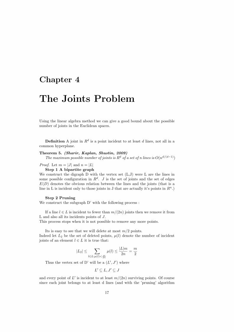
Using the linear algebra method we can give a good bound about the possiblenumber of joints in the Euclidean spaces.

Definition A joint in Rd is a point incident to at least d lines, not all in acommon hyperplane.

Theorem 5. (Sharir, Kaplan, Shustin, 2009)The maximum possible number of joints is Rd of a set of n lines is O(nd/(d−1))

Proof. Let m = |J | and n = |L|Step 1 A bipartite graph

We construct the digraph D with the vertex set (L,J) were L are the lines insome possible configuration in Rd. J is the set of joints and the set of edgesE(D) denotes the obvious relation between the lines and the joints (that is aline in L is incident only to those joints in J that are actually it’s points in Rn.)

Step 2 PruningWe construct the subgraph D’ with the following process :

If a line l ∈ L is incident to fewer than m/(2n) joints then we remove it fromL and also all its incidents points of J .This process stops when it is not possible to remove any more points.

Its is easy to see that we will delete at most m/2 points.Indeed let L2 be the set of deleted points, µ(l) denote the number of incidentjoints of an element l ∈ L it is true that:

|L2| ≤∑

l∈L:µ(l)< m2n

µ(l) ≤ |L|m2n

=m

2

Thus the vertex set of D’ will be a (L′, J ′) where

L′ ⊆ L, J ′ ⊆ J

and every point of L′ is incident to at least m/(2n) surviving points. Of coursesince each joint belongs to at least d lines (and with the ’pruning’ algorithm

17

18 CHAPTER 4. THE JOINTS PROBLEM

is continuing to be true in the remaining sub-configuration) each point of J’ isincident to at least d points of L′ (not all in the same hyper plane).

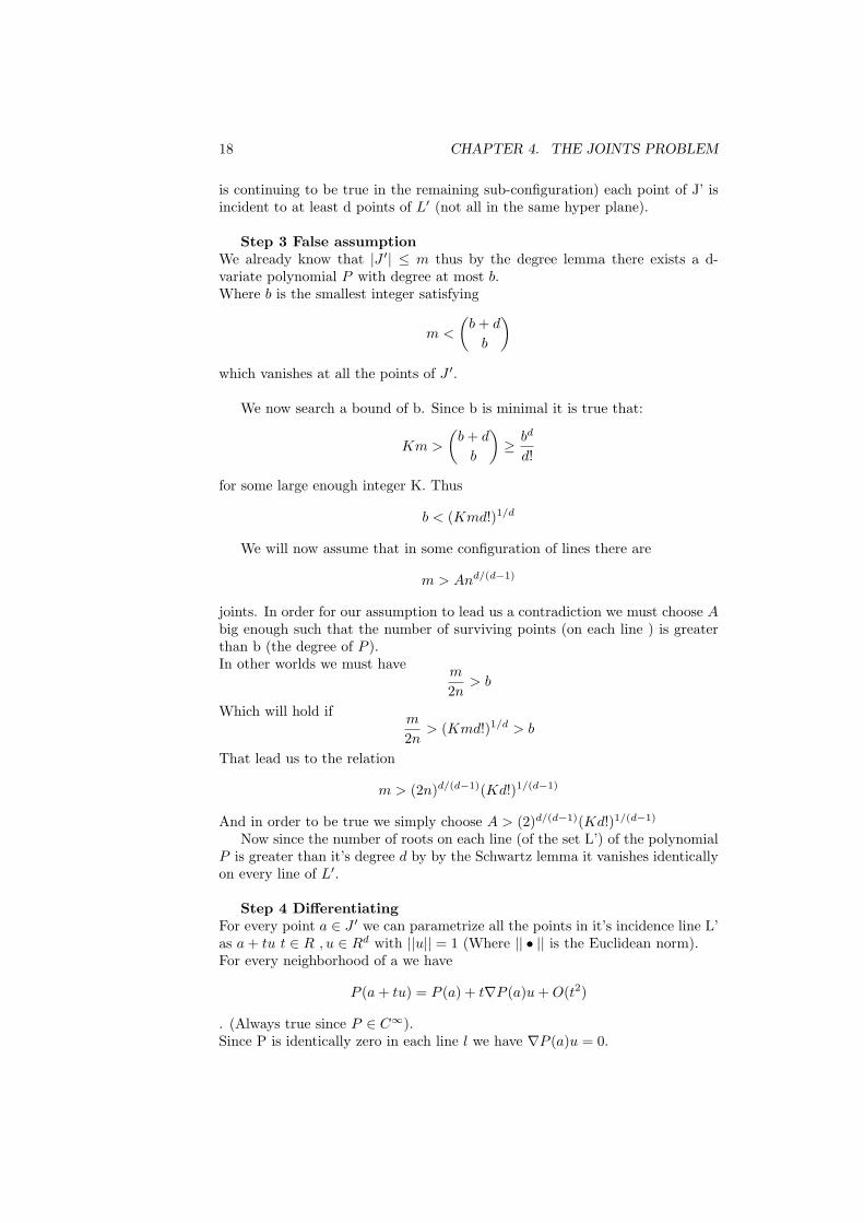
Step 3 False assumptionWe already know that |J ′| ≤ m thus by the degree lemma there exists a d-variate polynomial P with degree at most b.Where b is the smallest integer satisfying

m <

(b+ d

b

)which vanishes at all the points of J ′.

We now search a bound of b. Since b is minimal it is true that:

Km >

(b+ d

b

)≥ bd

d!

for some large enough integer K. Thus

b < (Kmd!)1/d

We will now assume that in some configuration of lines there are

m > And/(d−1)

joints. In order for our assumption to lead us a contradiction we must choose Abig enough such that the number of surviving points (on each line ) is greaterthan b (the degree of P ).In other worlds we must have

m

2n> b

Which will hold ifm

2n> (Kmd!)1/d > b

That lead us to the relation

m > (2n)d/(d−1)(Kd!)1/(d−1)

And in order to be true we simply choose A > (2)d/(d−1)(Kd!)1/(d−1)

Now since the number of roots on each line (of the set L’) of the polynomialP is greater than it’s degree d by by the Schwartz lemma it vanishes identicallyon every line of L′.

Step 4 DifferentiatingFor every point a ∈ J ′ we can parametrize all the points in it’s incidence line L’as a+ tu t ∈ R , u ∈ Rd with ||u|| = 1 (Where || • || is the Euclidean norm).For every neighborhood of a we have

P (a+ tu) = P (a) + t∇P (a)u+O(t2)

. (Always true since P ∈ C∞).Since P is identically zero in each line l we have ∇P (a)u = 0.

19

This holds for every (remaining) line incident to a. Since a is a joint we haveseen that there are at least d lines in L′.

(Which lines actually span the entire Rd). So ∇P (a) being orthogonal tothem all must be the zero vector.Thus all the first-order derivatives of P vanish at a .

Step 5 Final StepLets us now consider the derivatives Pxi

the degree is at most b− 1.Since:

a) Every line l ∈ L′ contains more than b− 1 points of J ′.

b) Pxivanishes at each and every point of those lines.

Then by Schwartz’s lemma Pxi must vanish identically on l.That means all the first-order derivatives of P vanish on all the lines of L′.We can repeat the above process to each of these derivatives and we can con-clude that all partial derivatives of P vanish identically on of lines off L′.This is impossible because eventually we must reach derivatives which arenonzero constants on Rd.

This is a contradiction.

Note. The original proof can be found in [4].

20 CHAPTER 4. THE JOINTS PROBLEM

Chapter 5

Discrete geometry problems

In this chapter we will examine some problems of the field of discrete geometryand in particular the Distance problem (defined below)

The distance problem Let

U = a1, a2, ..., am

be a set of points in the euclidean space Rn. For the euclidean distance we makeuse of the euclidean norm L2. Let A ∈ R be the set of all possible distances be-tween these points (the distance set). That is we have ||xi−xj || ∈ A ,with j 6= i.

LetK(n, l)

denote the maximal number m that there exists a family m of points U |U | =K(n, l) in Rn with distance set |A| = l we search bounds of the number K(n, l).

First we will see how the linear algebra method can be used to give boundsin some special cases.

Lemma 9. K(n,1)= n+ 1

Proof. We simply use the (n+1)-simplex polytope in every space Rn. Which is amaximal configuration (we cannot add more points to make it a (n+2)-simplex)and has (n+ 1) vertices.

Theorem 6. (Larman-Rogers-Seidel 1977)

K(n, 2) ≤(n

2

)+ 3n+ 2

21

22 CHAPTER 5. DISCRETE GEOMETRY PROBLEMS

Proof. We use the classic notation

||x|| = (n∑i=1

x2i )

1/2

for the Euclidean norm in Rn . Let U be a possible configuration of points Uin Rn.

This set U = a1, a2, ..., am gives birth to the following family of polynomialsF

fi(x) = (||x− ai||2 − d21)(||x− ai||2 − d2

2)

where d1, d2 are the elements of the two-point set A (the two possible dis-tances).We can easily see that

fi(aj) =

(d1d2)2 6= 0 if i = j;0 if i 6= j.

By the triangular criterion these polynomials are linearly independent.We now search the cardinality of the basis of (some) linear space in which

they reside. If we expand a polynomial fi of this family we can see that it is infact a linear combination of the following (linearly independent) polynomials

(n∑i=1

x2i )

2, (n∑i=1

x2i )xj , xixj , xi, 1

Using simple combinatorics to count their number we can see that theircardinality is actually

1 + n+ ((n

2

)+ n+ 1) =

(n

2

)+ 3n+ 2

The above number is the cardinality of the linear basis in question.

Since fi are linearly independent their number cannot exceed the cardinalityof their linear base this completes the proof.

Note The original proof can be found in [1].

We now make use of the linear algebra method for the general case K(n, s)

Theorem 7. (s-distance sets) Using the notation above for the number ofpoints K(n, s) we have(

n+ 1s

)≤ K(n, s) ≤

(n+ s+ 1

s

)

23

Proof. The upper bound Let y1, .., ym be a configuration of points in Rn

having the distance set A = d1, ..., ds.We once again construct the family F of polynomials

fi(x) =s∏

k=1

(||x− yi||2 − d2k)

and once again the polynomials fi are linearly independent. Let L be thelinear space which they generate.

We now search the cardinality of a basis of L. To do this we can use followingtrick.

1) We expand the norm-square expression in each factor of fi and collectthe squares. Thus the fi’s can be written as the sum of

(∑

x2i )k0xk11 ...x

knn with

n∑i=0

ki ≤ s

2) We set z =∑ni=1 x

2i

In this way the fi’s can be seen as polynomials of n+1 variables, with degreeat most s. The dimension of the linear space in which they reside is the numberof homogenous polynomials on n+ 1 variables and degree at most s. Since thisnumber is

(n+s+1

s

)we achieve the desired bound.

The Lower bound Let us consider the incidence vectors of all s-subsets ofa n+1 set. Let us name this set of vectors as W. This set lies on the hyperplanedefined by the equation

n+1∑i=1

xi = s

and therefore can be viewed as a subset of Rn.

It is easy to see that the cardinality of the distance set of the points of W isactually s. (The number of all possible different elements between 2 sets is aninteger a ∈ [0, ..., s]. ) Since the number of all s-subsets of a n+1 set is actually(

n+ 1s

)we have achieved the desired bound.

If the configuration of points is less general we can achieve tighter bounds.For example:

24 CHAPTER 5. DISCRETE GEOMETRY PROBLEMS

Theorem 8. (Spherical s-distance sets)The maximum cardinality Ks(n, s) of points in Sn−1 ⊂ Rn having distance setof size s is (

n+ 1s

)≤ Ks(n, s) ≤

(n+ s− 1

s

)+(n+ s− 2s− 1

)Proof. ( The radius of the sphere clearly does not matter. )

The lower bound We consider all the (1,-1)-vectors in Rn+1 with exactlys negative entries. Using simple combinatorics we can see that their number is(

n+ 1s

)Clearly all these points belong to a sphere

Sn ⊂ Rn+1

and they also belong to the hyperplane defined by the equation

n+1∑i=1

xi = n+ 1− 2s

And since the intersection of a hyperplane and a sphere is actually a sphere oflower dimension they can be viewer as a subset of

Sn−1 ⊂ Rn

And since their distance set is actually s (the number of all possible differentcoordinates between 2 points) we have achieved the lower bound.

The upper bound To achieve the upper bound we proceed as in the linearcase and construct a family D of linearly independent polynomials belonging toa linear space of the following base

(n∑i=1

x2i )n, (

n∑i=1

x2i )axk...xl, xi...xj , 1

For the next step we restrict the domain of the polynomials fi in the unitsphere. The functions will remain independent ( as members of the space ofSn−1 → R functions), but now we see that they reside in a lower dimensionalspace than before.

That is we can drop∑2i=1 from the list since it is a constant. We can also

drop x2kn since

x2n = 1−

n−1∑i=1

x2i

Thus the new base will have the following elements

xk11 ...xkn−1n−1 , xn(xb11 ...x

bn−1n−1 )

25

Withn−1∑i=1

ki ≤ s andn−1∑i=1

bi ≤ s− 1

The number of the above elements is(n+ s− 1

s

)+(n+ s− 2s− 1

)and the proof is complete.

More information about this family of problems can be found in [2]

26 CHAPTER 5. DISCRETE GEOMETRY PROBLEMS

Chapter 6

Extremal set theory

In this section we will use the polynomial technique to obtain some upper (andlower) bounds in the size of intersecting families.

Definition Let F be a family of subsets of some n-element set , and let

L ⊆ 0, 1, ...

be a finite set of nonnegative integers .We say that F is L-intersecting if

|A ∩B| ⊆ L

for every pair A,B of distinct members of F .

Theorem 9. (Frankl-Wilson 1981) If F is an L-intersecting family of sub-sets of a set of n elements, then

|F | ≤|L|∑i=0

(n

i

)Proof. (Due to Babai 1988. The original proof can be found in [2])

LetF = A1, ..., Am

be the family in question. Without loss of generality we can assume that

|A1| ≤ |A2| ≤ .... ≤ |Am|

LetL = l1, ..., ls

be the set of all intersection sizes. That is for every pair (i, j) with i 6= j thereis a k such that

|Ai ∩Aj | = lk

27

28 CHAPTER 6. EXTREMAL SET THEORY

We will now associate each set Ai with its incidence vector ui = (ui1, .., uin),which we define as

uij =

1 if j ∈ Ai;0 if j /∈ Ai.

It is easy to see that|Ai ∩Aj | = 〈ui, uj〉

where the form

〈x, y〉 =n∑i=1

xiyi

is the standard inner product in Rn.

For our next step we construct the following family F of polynomials fi foreach i = 1, ...,m

fi(x) =∏

k:lk<|Ai|

(〈ui, x〉 − lk)

(We choose x ∈ Rn so that the above polynomials fi will be n-variable andwell defined.)We observe that

fi(uj)6= 0 for all 1 ≤ i ≤ m, i = j ;= 0 for all 1 ≤ j < i ≤ m .

By the diagonal criterion the polynomials f1, f2, ..fm are linearly indepen-dent.

We now search for the cardinality of a basis of the linear space F. Becausethe domain (of the polynomials ) is actually 0, 1 we have x2

i = xi for eachvariable xi.

Thus we see that all the f ′is can be represented as sum of monomials . Andwe can see also that all the f ′is have degree at most s = |L| (due to the fact sis the number of all possible intersection sizes).

Thus the set of all monomials on (at most) n variables and degree (at most)s are a basis of the linear space F .

We can easily see that we have at mosts∑i=0

(n

i

)of them, so the proof is complete.

Using the same arguments we can prove the modular variation of the abovetheorem.

29

Theorem 10. (Deza-Frankl -Singhi 1983)Let L ⊆ 0, 1, .., p − 1 and p be a prime number. Assume that F =

A1, .., Am is a family of subsets of a set of n elements such that:

(a) |Ai| /∈ L (mod p) when (1 ≤ i ≤ m);(b) |Ai ∩Aj | ∈ L (mod p) when 1 ≤ j < i ≤ m).Then

|F | ≤|L|∑i=0

(n

i

)Proof. We begin with a simple observation. Recall that a polynomial is multi-linear if it has degree ≤ 1 in each variable. Every multi-linear polynomial ofdegree ≤ s is a linear combination of monic multi-linear monomials (productsof distinct variables) of degree ≤ s.We will also make use of the following lemma:

Lemma 10. (Multilinearization) Let F be a field and Ω = 0, 1n ⊆ Fn. Iff is a polynomial of degree ≤ s in n variables over F then there exists (unique)multi-linear polynomial f ′ of degree ≤ s in the same variables such that

f(x) = f ′(x) for every x ∈ Ω

Proof. To prove this one can just expand f and use the identity x2i = xi, valid

over Ω

We once again introduce a polynomial F (x, y) in 2n variables , this timex, y ∈ Fnp ,where Fnp is the linear space of dimension n over Fp. We set

F (x, y) =∏l∈L

(x · y − l)

where

x · y =n∑i=1

xiyi

is the standard inner product in Fnp . Now consider the n-variable polynomials

fi(x) = F (x, ui)

whereui ∈ Fnp

is the incidence vector of the set

Ai (i = 1, ...,m)

. It is clear from the conditions that for 1 ≤ i, j ≤ m

fi(uj)6= 0 if i = j;= 0 if i 6= j.

These equations remain valid if we replace the fi by the corresponding linearpolynomials f ′i .By the diagonal criterion these polynomials are linearly independent over Fp.

30 CHAPTER 6. EXTREMAL SET THEORY

On the other hand all the f ′i are multi-linear polynomials of degree ≤ s andtherefore belong to a space of dimension

|L|∑k=0

(n

k

)

Theorem 11. (Bollobas). The original proof can be found in [1]. LetA1, ..Am be sets of size r and B1, ..Bm be sets of size s such that

(a) Ai ∩Bi = ∅ for i = 1, ..,m(b) Ai ∩Bj 6= ∅ whenever i 6= jthen we have

m ≤(r + s

s

)Proof. (Due to Frankl )Let X be the union of all sets Ai ∪ Bi. Let T (X) be an enumeration of theelements of X. We associate each x ∈ X with a vector

F : x→ 〈1, T (x), ..., T r(x)〉

Every r + 1 of these vectors are linearly independent, since (1, T (x), ..., T r(x))are points in the moment curve (1, t, ..., tr) ⊆ Rr+1.

Now each subset W ⊂ X we associate it with a polynomial fW (y) of r + 1variables in the following way:

fW (y) =∏u∈W

(y · F (u))

It is easy to see that fBj(x) = 0 if and only if F (u) · x = 0 for some u ∈ Bj .

The vectors corresponding to the elements of Ai generate a sub-space Si ofdimension r. Let ai be a nonzero vector orthogonal to Si.

From b follows that fBi(aj) = 0 if i 6= j. Since every r+ 1 vectors F (x), x ∈

X are linearly independent it follows from a and the fact that dim(Si) = r that

dim(〈F (Ai) ∪ F (Bi〉) = r + 1

From the above and since ai is a non-zero vector orthogonal to Si we concludethat fBi

(ai) 6= 0.

Thus by the diagonal Criterion the polynomials are linearly independent.And since they are homogenous of degree s in r+ 1 variables their number is atmost (

(r + 1) + s− 1s

)and the proof is complete.

31

Theorem 12. (Nonuniform Fisher Inequality ) Let Ci, ..., Cm be distinctsubsets of a set of n elements satisfying the following condition :|Ci ∩ Cj | = λ for some integer λ with 1 ≤ λ < n and for every i 6= j Then

m ≤ n

Proof. First we separate the case that one of the sets Ci has λ elements. Thenall the others must contain this one and be disjoint otherwise. It follows that

m ≤ n+ 1− λ ≤ n

The second case will be that all the sets in question have more than λ elementsthat is that the numbers

γi = |Ci| − λare all positive.

We construct the incidence matrix M of the set system. (Where Mij = 1if the jth element belongs to the ith set, and zero otherwise ). This conditioncan be summarized in the following matrix equation :

A = MMT = λJ + C

where J is the all ones m×m matrix and C is the diagonal matrix

C = diag(γ1, ..., γm)

We will now prove that A is of full rank. We will make use of the followinglemma.

Lemma 11. All positive definite matrices have full rank .

In order to use the above lemma we will prove that λJ is positive semidefiniteand C is positive definite. Indeed let

x = (x1, ..., xm) ∈ Rm

For a m×m matrix U = (µij) we have

xUxT =m∑i=1

m∑i=1

µijxixj

ThusxλJxT = λ(x1 + ...+ xm)2

AndxCxT = γ1x

21 + ...+ γmx

2m

which justify both claims . Now it is obvious by the definition in chapter [2]that the sum of a positive definite and a positive semidefinite matrix is positivedefinite. Thus A is positive definite , thus it has full rank . Now we can see that

m = rk(A) ≤ rk(MMT ) ≤ rk(M) ≤ n

and the proof is complete .

32 CHAPTER 6. EXTREMAL SET THEORY

Chapter 7

Hilbert’s Third problem

The first of the famous Hilbert’s problems that was solved was Problem 3.Although the first proof was complicated we will present a greatly simplifiedone in the spirit of the previous chapters.

First we will need some definitions.

Definition 2. We call two polyhedra in R3 equidissectible if one can dissecteach of them by a finite number of plane cuts so that the resulting two sets ofsmaller polyhedra can be paired off into congruent pairs . In other words , onecan cut up one of them and then reassemble the pieces to obtain the other

Theorem 13. (M. Dehn, 1900) There are two polyhedra in R3 that are notequidissectable.

Proof. In order to prove the above theorem we will need the following fact. Let

a = arccos(1/3)

Then a/π is irrational.

Proof. Suppose the contrary. Then there exist positive integers k, l such thata/π = k/l. Thus

a =k

lπ ⇒ eai = e

kl πi ⇒ (eai)2l = e2kπ1 = 1

1 = (eai)2l = (13

+

√1− 1

32i)2l = (

13

+√

83i)2l

Now we claim that

(13

+

√1− 1

32i)n =

an3n+1

+√

2bn3n+1

i

This is true for n = 1. Suppose it holds for n− 1. Then

(13

+

√1− 1

32i)n = (

an−1

3n+1+√

2bn−1

3n)(

13

+√

83i)

33

34 CHAPTER 7. HILBERT’S THIRD PROBLEM

Multiplying out the right hand side, one arrives at the formulas an =an−1 − 4bn−1 and bn = bn−1 + 2an−1.

Note that a1 = 1 and b1 = 3 = −1 mod(3) . Plugging into the aboverecursions, we see that a2 = −1 mod(3) and b2 = 1 mod(3) . Plugging in oncemore we get a3 = 1 mod(3) and b3 = −1 mod(3) , whereupon the cycle repeats.In particular, bn is never congruent to zero modulo three. which leads us tocontradiction. Thus the proof is complete.

A dihedral angle is the angle subtended by two half-planes with a commonbounding line (the “spine”). Let as consider the following two polyhedra in R3

:

a) The regular simplex.

b) The cube .

Using simple analytic geometry we see that all the dihedral angles at theedges of the cube are π/2 radians , and the for the angles of the regular simplex(at it’s edges ) are a radians.

We assume (for a contradiction ) that the regular simplex and the cube areequidissectible. Let b1, ..., bm be all the dihedral angles that occur at edges ofthe smaller polyhedra obtained in the course of dissection. Let V denote theset of all linear combinations of the bi with rational coefficients. Then V is a(finite dimensional) linear space over Q. Therefore, it follows that there existsa linear function

f : V → Q

such that f(π) = 0 and f(a) = 1. We also note that f(π/2) = 0 follows.

Let us now consider, for each polytope P arising in the dissection processthe so-called Dehn invariant of P with respect to f:

W (P ) =∑|ei|f(ci)

where the summation extends over all edges ei of P, |ei| denotes the length ofei and ci is the dihedral angle of P at ei.

Lemma 12. The Dehn invariant is additive.

In other words if we cut a polyhedron to pieces, the W-values of the piecesadd up to the W-value of the whole.

Proof. It suffices to prove this for a single cut

P = Pi ∪ P2

where the two pieces are cut apart along a plane S and have disjoint interiors.We will show that

W (P ) = W (P1) +W (P2)

35

Let us expand each term above and examine what happens to the terms on theleft hand side of the resulting equation.

The terms corresponding to edges not cut by S show up intact on the righthand size. If S cut across some edge ei, it divides ei , into two pieces both stillattach to the same dihedral angle ci, so the corresponding two terms on theright hand side add up to |ei|f(ci). If cuts into the spine (the edge ei lies in thehyperplane S) then S splits the dihedral angle ci and leaves the ei unaltered.The additivity of f guarantees the that the balances of the two sides is onceagain maintained.

Finally, we have to consider the contribution of the new edges arising alongS but not appearing along P. Let e be such an edge (common in P1 and P2 )and ci the corresponding dihedral angle in Pi. It is obvious that

c1 + c2 = π

. Therefore the contribution of this edge is

|e|f(c1) + |e|f(c2) = |e|f(c1 + c2) = |e|f(π) = 0

This completes the proof of the additivity lemma .

The following corollary is immediate.

Corollary 1. If two polyhedra are equidissectible then they have the same Dehninvariants

For the final step we see that the Dehn invariant of the cube is 0 (sincef(π/2) = 0) , while the Dehn invariant of the regular simplex is not (sincef(a) 6= 0 ) The proof is complete .

36 CHAPTER 7. HILBERT’S THIRD PROBLEM

Chapter 8

References

1. S. Jukna , Extremal Combinatorics , Springer-Verlag , 2001

2. L. Babai and P. Frankl , Linear Algebra Methods in Combinatorics ,Preliminary Version , University of Chicago , 1992

3. R.A. Brualdi, Introductory Combinatorics , Fourth Edition , Prentice Hall, 2004

4. Z. Dvir , On the size of Kakeya sets in finite fields , arXiv:0803.2336v3

5. L. Li , On the size of Nikodym sets in finite fields , preprint

6. T. Wolff , Recent work connected with the Kakeya problem , Prospects inmathematics , 129 - 162 , Amer. Math . Soc. , Providence ,RI, 1999.

7. L. Guth , H. Katz , Algebraic Methods In Discrete Analogs Of The KakeyaProblem , arXiv:0812.1043v1

37